The Application of an Empirical Method for the Estimation of Vehicles’ Contribution to Air Pollution in an Urban Environment: A Case Study in Athens, Greece

Abstract

This research focuses on monitoring and analyzing air pollutant emissions, mainly from passenger vehicles, at a busy urban intersection with 19 traffic lanes at the junction of Thivon Avenue and Iera Odos, located in the Egaleo municipality, an urban region of Athens, Greece. To collect data, a monitoring study was conducted specifically on the four central traffic streams of this specific intersection. On each segment of the road, a specific length was assigned through which vehicles pass at an average speed in order for their emissions to be estimated. For each vehicle, the engine type (gas or diesel) and engine displacement were taken into account to calculate the predicted mass of vehicle emissions. These measurements were conducted separately for each segment and recorded during three signal phases (from green to red) for two weekdays and one non-working day. This approach allows pollutant levels to be monitored at various hours and under various traffic conditions. The analysis revealed not only the overall quantity of emissions from vehicles but also their fluctuations throughout the day and traffic conditions, comparing them with the regulatory limits set by the EU. Significant findings regarding the impact of traffic on air quality are highlighted.

1. Introduction

Air pollution is a major environmental and public health concern in urban areas worldwide. The European Environmental Agency (EEA) reported that in 2022, despite continued declines in emissions, a significant part of the EU’s urban population remained exposed to harmful levels of key air pollutants. Specifically, nearly all urban residents experienced PM_2.5 concentrations exceeding the 2021 WHO annual guideline of 5 µg/m³, as well as ozone (O₃) levels surpassing the short-term guideline of 100 µg/m³ [1]. One of the predominant sources of air pollution in cities is road transport, since a variety of pollutants, including nitrogen oxides (NO_X), carbon monoxide (CO), volatile organic compounds (VOCs), and particulate matter (PM), are emitted from vehicles [2]. These pollutants contribute to poor air quality [3], adversely affecting human health [4,5], ecosystems, and climate. The relationship between traffic and air pollution has been extensively studied, highlighting the role of vehicular emissions in the degradation of urban air quality [6,7,8,9]. In densely populated cities with high vehicular densities, traffic-related pollution can reach critical levels, posing significant challenges for policymakers and urban planners. This is because vehicles operating under stop-and-go conditions exhibit increased fuel consumption and higher emission rates compared to those in free-flowing traffic. Several parameters contribute to traffic congestion, including road infrastructure limitations, rapid urbanization, population growth, and inefficient public transportation systems. Additional factors such as traffic signal inefficiencies, driver behavior, and meteorological conditions further exacerbate congestion, exhaust and non-exhaust road emissions [10], and their environmental consequences. The road network capacity is also a fundamental aspect of urban planning that shapes city infrastructure and influences the sustainability of transportation systems. Understanding the contribution of road transport to air pollution requires a detailed analysis of the abovementioned parameters and the application of reliable methodologies for the estimation of emissions and the consequent impacts [11].

Various empirical and computational methods have been developed to assess road transport emissions and their impact on urban air quality. These methods range from direct measurement techniques, such as roadside monitoring and remote sensing, to modeling approaches that estimate emissions based on traffic data, fuel consumption, and vehicle fleet composition [12,13,14,15,16]. These methodologies enable researchers and policymakers to quantify the contribution of vehicles to air pollution, identify pollution hotspots, and develop mitigation strategies.

However, ref. [17] highlighted critical issues in existing approaches, such as the lack of clear and universally accepted definitions of traffic congestion, leading to inconsistencies in research findings. Additionally, this study pointed out that many models fail to incorporate real-world traffic conditions, such as speed fluctuations and vehicle dynamics. This research introduced an innovative model linking average travel speed with maximum traffic capacity, offering practical solutions for urban transport systems.

Traffic congestion is closely related to air quality, especially in areas with high traffic density near major roadways. The authors of [18] investigated the impact of traffic density parameters on air pollution, focusing on indicators such as Main Road Density (MRD), Average Traffic Density (ATD), and Heavy Vehicle Density (HTD). Their findings emphasize that these parameters significantly influence pollutant concentrations. This underscores the importance of integrating real-time traffic indicators into air pollution risk assessments. Several studies have examined how specific traffic parameters affect vehicle emissions [19,20,21,22] and references therein]. Traffic speed and acceleration fluctuations are key determinants of pollution levels, as they directly impact fuel consumption and emission rates per kilometer traveled. Sun, Bao, and colleagues [23] investigated the impact of traffic and urban structure on lung cancer incidence in high-density areas. Their findings revealed strong correlations between socioeconomic factors, pollution levels, and public health, emphasizing the need for a multifactorial approach to urban planning and pollution control. These results suggest that beyond managing traffic flow and road capacity, land-use planning should also aim to minimize the effects of vehicle emissions on residential areas.

Athens, Greece, is an ideal case study subject for examining the impact of vehicular emissions on urban air quality due to its high traffic congestion levels and historical air pollution problems. The city has long struggled with elevated concentrations of pollutants such as nitrogen dioxide (NO₂) and fine particulate matter (PM_2.5), often exceeding European Union (EU) air quality standards [24,25,26]. The complex topography of Athens, surrounded by mountains, further exacerbates air pollution by limiting atmospheric dispersion. Traffic congestion in the city is a persistent issue, driven by high car ownership rates, an aging vehicle fleet, and insufficient public transport infrastructure. Progiou and Ziomas [27] highlighted that emissions from older vehicles disproportionately contribute to pollution levels, emphasizing the need for targeted policies to renew vehicle fleets and implement emission control strategies. These factors make Athens a representative example of an urban environment where road transport significantly contributes to air pollution, necessitating the application of empirical methods for emission estimation and control strategies.

The use of dynamic systems for monitoring and predicting pollution offers innovative approaches to managing traffic congestion. Shepelev et al. [28] introduced a dynamic monitoring system using data to analyze the correlation between traffic speed and pollutant emissions. Their study demonstrated that lower speeds and frequent stops at intersections contribute to higher emissions, particularly from older vehicles with less efficient combustion systems. Inspired by their research, the present study focuses on monitoring vehicle emissions at the intersection of Thivon and Iera Odos Str., in the municipality of Egaleo, a suburban area of Athens, Greece. By incorporating real-time data and predictive models, the scope of this study is to identify the factors influencing air pollution and propose actionable solutions to mitigate traffic-related pollution while promoting sustainable policies.

2. Materials and Methods

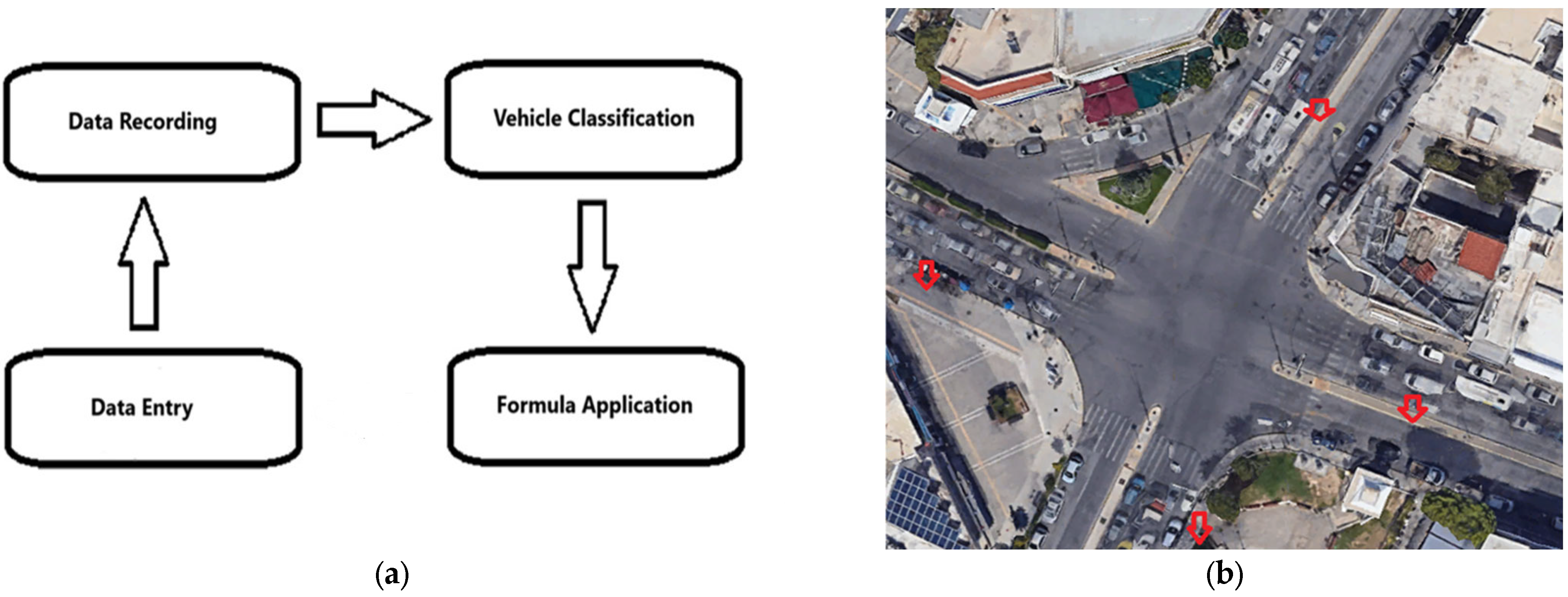
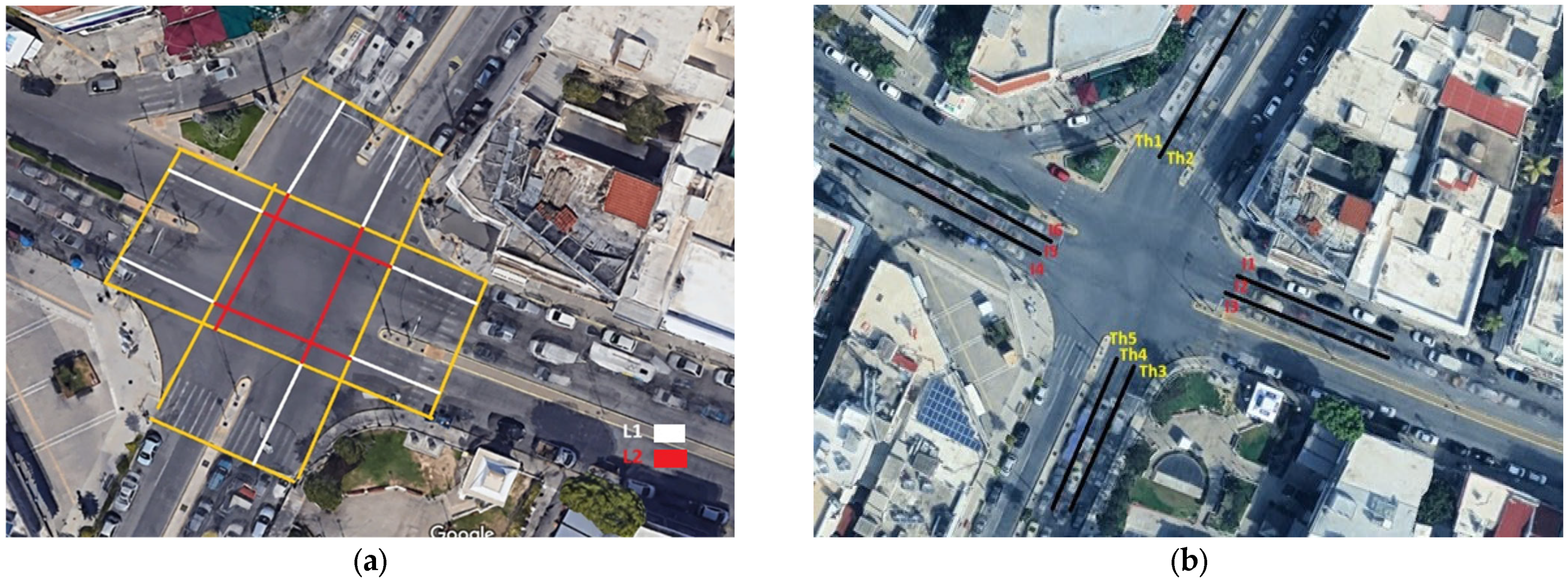
2.1. Study Area and Data Collection

This study was conducted at the intersection of Thivon and Iera Odos Str., a busy urban junction with a high traffic density of passenger vehicles, aiming to quantitatively assess the pollutant emissions produced by passing vehicles (Figure 1b). Data collection (

Table 1. Data collection characteristics (date and period and weather conditions).

	Date	Time	Weather Conditions	Temperature (°C)
1st	18 December 2023	07:30–08:00 a.m.	Light cloud cover with sunshine.	8
2nd	22 December 2023	05:30–06:00 p.m.	Light cloud cover/sunset.	12
3rd	8 January 2023	07:30–08:00 a.m.	Light cloud cover without sunshine.	7
4th	14 January 2023	07:30–08:00 a.m.	Light cloud cover with minimal sunshine.	6

) was carried out through video recording from selected vantage points around the intersection.

The video recording process captured all three phases of traffic light operation (green, amber, red), ensuring the documentation of vehicle traffic under varying traffic signal conditions. Recording was conducted over a two-week period, covering both peak and off-peak hours to collect representative traffic flow data under diverse conditions. The collected footage was analyzed using video and image processing software, allowing for the identification and classification of vehicles based on engine type (benzine or diesel) and engine displacement (small- or medium-sized engines) (

Table 2. Total number of vehicles per type of fuel and day (working and non-working).

	Benzine		Diesel
	Small Vehicles	Medium Vehicles	Small Vehicles	Medium Vehicles
Working day	383	121	165	32
Non-working day	56	4	25	3

). Additionally, the speeds of vehicles passing through the intersection were recorded, as speed is a critical parameter for estimating pollutant emissions. The data obtained from the analysis were subsequently used in mathematical models to calculate total pollutant emissions, as well as emissions with respect to vehicle category and pollutant type. The data collection and analysis process stages are illustrated in Figure 1a.

This systematic approach ensured the repeatability of the method and the accuracy of the results.

2.2. Materials and Equipment and Variable Selection

The lanes at the intersection were analyzed individually and categorized based on their common characteristics to ensure the accuracy and reliability of the results. This categorization can facilitate the application of this study’s findings to other intersections or road networks with similar characteristics. The key parameters used for the lane analysis included lane capacity, saturation flow, lane length, and vehicle speed. These variables are essential for understanding traffic flow and accurately estimating pollutant emissions, enabling this study to be replicated and its methodology applied to similar traffic environments.

Table 3. Parameters, descriptions, equations, and units.

Parameter	Description	Equation/Values
L1	Distance from the stop line to the 1st conflict point of the intersection.	(m)
L2	Distance from to the 1st conflict point to the end of the intersection (2nd conflict point).	(m)
Cij	Lane capacity: maximum number of vehicles passing during one signal cycle, where $g_{ej}$ represents the number of seconds during which the traffic signal indication lasts, and c represents the total number of recorded signal phases.	$C_{ij}={\displaystyle \frac{Sij\ast gej}{c}}$
Sij	Saturation flow rate for lane i during signal phase j.	$S_{ij}=S_o\ast \mathrm{N}\ast f_W\ast f_{HV}\ast f_G\ast f_P\ast f_{BB}\ast f_A\ast f_{RT}\ast f_{LT}$
$S_o$	Saturation flow rate depending on lane width.	Lane widths in the following ranges: 0–2.9 m: $S_o$ = 1.736–1.752 3–3.6 m:$S_o$ = 1.815–1.830 3.7–4 m: $S_o$ = 1.898–1.913
$f_W$	Adjustment factor for lane width.	Up 3.5 m = 0.96, >4 m $f_W$ = 1
N	Number of vehicles passing through each signal phase per lane.	-
$N_m$	Number of vehicles overtaking a parked vehicle.	-
$f_G$	Adjustment factor for lane gradient.	$f_G={\displaystyle \frac{1-P_G}{200}}$, $P_G$ road slope (degrees)
$f_P$	Adjustment factor for the effects of parked vehicles.	$f_P={\displaystyle \frac{N-0.1-\frac{18N_m}{3600}}{N}}\ge 0.05$
$f_{BB}$	Adjustment factor for the effects of public transportation (not considered in this study).	$f_{BB}={\displaystyle \frac{N-\frac{14.4N_b}{3600}}{N}}\ge 0.05$
$f_{RT}$ and $f_{LT}$	Adjustment factors for the effects of right-turning and left-turning vehicles.	$f_{RT}={\displaystyle \frac{1}{E_r}}$, $E_r$=${\displaystyle \frac{Vehiclesturningright}{Totalvehicles}}$ $f_{LT}={\displaystyle \frac{1}{E_r}}$, $E_r$=${\displaystyle \frac{Vehiclesturningleft}{Totalvehicles}}$

presents the data used for the lane analysis [29,30].

Focusing on the measurements conducted over a two-week period, this experiment provides an initial stage for calculating pollutant emissions from vehicles traveling at a constant speed as they pass through the controlled intersection, based on factors associated with the traffic lanes. The video recording points were strategically selected primarily at locations where vehicles come to a stop during the red light phase in each traffic stream (Figure 2a). This specific recording strategy enables the accurate collection of data on traffic flow and vehicle behavior, supporting the precise estimation of pollutant emissions.

For the optimal processing of the data related to vehicle flow in each traffic stream, the lanes were grouped based on their shared characteristics (Figure 2b). Grouping the lanes into specific categories allows for easier data analysis and the extraction of reliable results. To facilitate this analysis, names were assigned to each lane group, which were consistently used throughout this study. This methodology enables the generalization of the results and their application to other intersections with similar traffic characteristics. The naming conventions used for each lane group are outlined below [29,30].

This study analyzed the traffic lanes of Thivon Street and Iera Odos, examining their respective characteristics and gradients. For Thivon Street, five lanes were evaluated, named Th1, Th2, Th3, Th4, and Th5 (Figure 2b). All these lanes are part of the traffic flow in both directions of Thivon Street. The road gradient for these lanes was determined to be flat, meaning it was neither uphill nor downhill. According to the gradient limits (−6 ≤ P_g ≤ 10), the gradient was assigned a value of P_g = 0°. Similarly, for Iera Odos, five lanes were analyzed, named Ι1, Ι2, Ι3, Ι4, and Ι5 (Figure 2b), which are also part of the traffic flow in both directions of Iera Odos. The road gradient for these lanes was also determined to be flat, with a gradient value of P_g = 0° in alignment with the same limits (−6° ≤ P_g ≤ 10°). For the purposes of the present study, the consistent road gradient across all lanes ensures uniform traffic flow characteristics, and the lanes analyzed share common characteristics. The intersection length is divided into two segments, L1 and L2, to enhance measurement accuracy. L1 represents the distance from the stop line to the first conflict point, while L2 covers the distance from the first conflict point to the end of the intersection, enabling a more detailed analysis of the area. The saturation flow rate is adjusted according to the width of each lane, with wider lanes allowing for more vehicles per hour and thus improving traffic flow capacity. The theoretical lane capacity reflects the maximum number of vehicles that can pass through a lane in a specific time frame, influenced by the saturation flow rate and the green phase duration of the traffic signal. Additionally, all lanes are impacted by external factors such as the consistent and flat road gradient, parked vehicles that may reduce traffic flow, and traffic flow influences from turns, including right and left turns.

Once the lanes are classified and grouped, a methodology for calculating the total pollutant emissions is applied based on estimating the emissions for each vehicle type individually and subsequently summing up the total emissions. Calculations were made by categorizing vehicles according to their type, such as benzine and diesel vehicles. The primary types of emissions studied were those of particulate matter (PM), carbon monoxide (CO), nitrogen oxides (NO_X), and Non-Methane Volatile Organic Compounds (NMVOCs) [30].

Afterward, the transit time for each vehicle crossing the examined lane section is determined by calculating the difference between its entry and exit times. To finalize the calculation, total emissions are derived by summing the recorded values for all vehicles and applying a correction factor that accounts for traffic flow speed.

The equation used for calculating the total emissions M_LV (g/s) is expressed as follows [28]:

$$M_{LV}={\int }_0^t{\displaystyle \frac{L_0}{1200}}\sum {\displaystyle \frac{M_{k,i}\ast G_k}{L_o}}\ast \int r_V\left[V\right(t\left)\right]dt$$

(1)

where the variables are defined as follows:

Lo is the length of the road section under examination.

$M_{k,i}$ represents the emissions of pollutant i from vehicle type k.

G_k is the traffic intensity for each vehicle type k (measured in vehicles per hour).

r_v[V(t)] is the emission adjustment factor (

Table 4. Correction factor rv [V(t)].

Vi (km/h)	rV[V(t)]
5	1.4
10	1.35
15	1.3
20	1.2
25	1.1
30	1.0
35	0.9
40	0.75
45	0.6
50	0.5
60	0.3

). It is based on the traffic flow speed V_i, which is derived from the experimental data [28]. More specifically, the speed V_i was calculated using the average travel time of vehicles passing through the examined road segment, using the following equation:

$$\mathrm{V}={\displaystyle \frac{L_0}{t}}$$

(2)

where t is the average travel time

2.3. Emission Calculation

This study included benzine- and diesel-powered vehicles, referring to those that use benzine and diesel as their primary fuel sources, without any auxiliary propulsion systems such as hybrid technologies. These two categories were further divided into two subcategories based on engine displacement: small- and medium-sized vehicles. Vehicles with an engine displacement ranging from 900 cc to 1400 cc were classified as small, while those with an engine displacement ranging from 1401 cc to 2000 cc were classified as medium.

Data collection began with the recording of a regulation cycle, consisting of three signal phases. Each signal phase represents the time interval between two consecutive changes in the traffic light at the intersection and refers to the lanes affected by the respective traffic signal. During each signal phase, the number of vehicles passing through the intersection was recorded and categorized into the aforementioned groups. The following Table 4,

Table 5. Average vehicle emissions per kilogram of fuel consumed (g/kg).

Pollutant	Small Benzine	Medium Benzine	Small Diesel	Medium Diesel
PM	0.02	0.04	0.8	2.64
CO	49	84.7	2.05	8.19
NOx	4.48	29.89	11.2	13.88
NMVOCs	5.55	34.42	0.41	1.88

and

Table 6. Average fuel consumption per vehicle type (Lit/km).

Small Benzine	Medium Benzine	Small Deisel	Medium Deisel
0.06	0.08	0.05	0.07

display the calculated and recorded data, where emissions are presented separately per lane and per vehicle category at the intersection. The pollutants emitted per kilogram of fuel consumed from each vehicle type are presented in Table 5. It should be mentioned that these values refer to the average emissions, and the detailed methodology for their calculation is referred to in [30].

Keeping in mind the emissions for each engine per kilogram of fuel consumed, the calculation of emissions per kilometer traveled is conducted by using the average fuel consumption per kilometer for each type of vehicle [30] and the fuel density of benzine and diesel in kilograms per liter (Table 6) [31].

Fuel density was a key parameter used in the calculation of pollutant emissions per type of fuel [30]. Specifically, the following values were found:

• For benzine, the density was measured at 0.74 kg/Lit, indicating that each liter of diesel weighs 0.74 kg.
• For diesel, the density was measured at 0.88 kg/Lit, indicating that each liter of diesel weighs 0.88 kg.

To calculate the emissions for each pollutant per kilometer and per vehicle, we use the following formula:

Pollutant_{((g/km)/Vehicle)} = Pollutant_{((g/kg)/Vehicle)} × Average Consumption _(Lit/km) × Fuel Density_(kg/Lit)

(3)

Depending on the fuel category under study, we use the respective values (0.74 kg/Lit for benzine and 0.88 kg/Lit for diesel). As a result, the table below is produced (

Table 7. Average vehicle emissions (g/km).

Pollutant	Small Benzine	Medium Benzine	Small Diesel	Medium Diesel
PM	0.001	0.002	0.035	0.163
CO	2.176	5.014	0.090	0.505
NOx	0.199	1.769	0.493	0.855
NMVOCs	0.246	2.038	0.018	0.116

).

These values were utilized alongside the average fuel consumption of vehicles to calculate emissions per kilometer traveled.

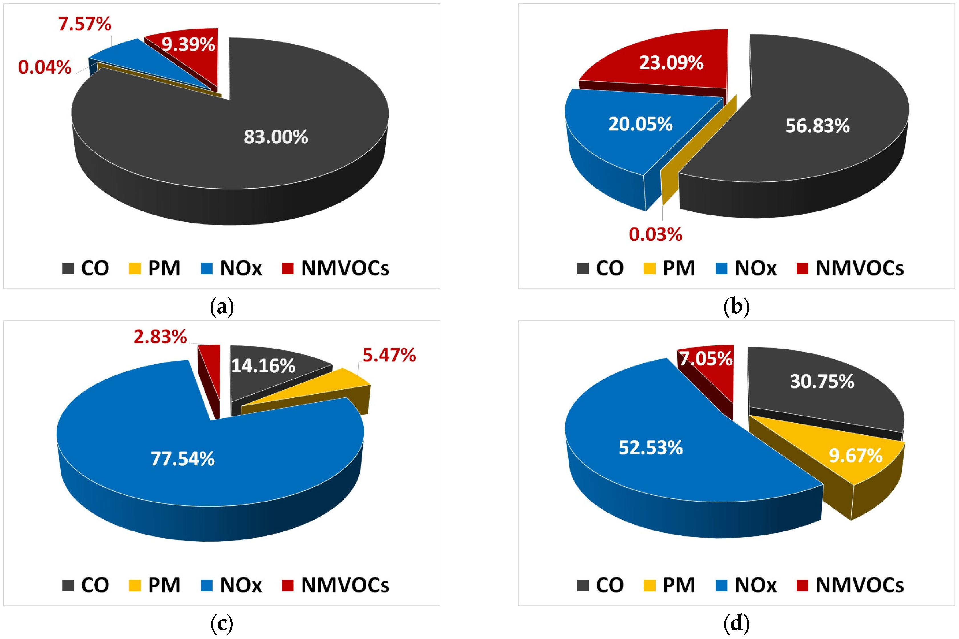
3. Results and Discussion

Based on the above methodology, the mass (gr) of pollutant emissions was calculated for both working and non-working days. The calculations concern the time period between a signal phase, which is the time interval between two consecutive changes in the traffic light at the intersection for all directions and lanes.

On working days and hours, due to the coverage of the right part of the roadway in both directions by parked vehicles, traffic jams are caused. This results in a much smaller number of cars passing through in each phase of the traffic lights (from green to red) at a very low speed, thus increasing pollutant emissions, compared to Sunday where there is no traffic jam and vehicles pass through the intersection at a higher speed and in a larger number, in each phase of the traffic lights.

Table 8. Estimated emitted mass (gr) of PM.

	Benzine		Diesel
	Small Vehicles	Medium Vehicles	Small Vehicles	Medium Vehicles
Working day	0.0048	0.0029–0.0059	0.0549–0.0995	0.0550–0.0959
Non-working day	0.0021	0.0004	0.0371	0.0207

,

Table 9. Estimated emitted mass (gr) of CO.

	Benzine		Diesel
	Small Vehicles	Medium Vehicles	Small Vehicles	Medium Vehicles
Working day	10.84–12.40	6.14–12.96	0.15–0.25	0.17–0.31
Non-working day	5.14	0.84	0.10	0.06

,

Table 10. Estimated emitted mass (gr) of NO_X.

	Benzine		Diesel
	Small Vehicles	Medium Vehicles	Small Vehicles	Medium Vehicles
Working day	0.99–1.13	2.17–4.57	0.80–1.39	0.29–0.53
Non-working day	0.47	0.30	0.52	0.11

and

Table 11. Estimated emitted mass (gr) of NMVOCs.

	Benzine		Diesel
	Small Vehicles	Medium Vehicles	Small Vehicles	Medium Vehicles
Working day	1.23–1.40	2.49–5.27	0.03–0.05	0.04–0.07
Non-working day	0.58	0.34	0.02	0.01

depict the estimated emitted mass (gr) for each pollutant for each the examined vehicle type and for both working and non-working days.

On working days and hours, compared to non-working days, PM emissions are increased from approximately 150% (small vehicles) to 1000% (medium vehicles).

According to Table 9, CO emissions on working days and hours, compared to non-working days, are increased from approximately 130% (small benzine engine vehicles) to 1400% (medium benzine engine vehicles). Concerning the diesel engine vehicles, CO emissions are increased from approximately 100% (small vehicles) to 300% (medium vehicles). It seems that diesel engine vehicles emit less CO compared with the corresponding benzine engine vehicles.

Table 10 depicts the NO_X emissions. On working days and hours, compared to non-working days, NO_X emissions are increased from approximately 125% (small benzine engine vehicles) to 1000% (medium benzine engine vehicles). Concerning diesel engine vehicles, NO_X emissions are increased from approximately 110% (small vehicles) to 270% (medium vehicles). During non-working days, there are no significant differences for NO_X emissions between benzine and diesel engine vehicles.

Table 11 shows the NMVOC emissions on working days and hours, compared to non-working days. According to Table 11, NMVOC emissions are increased from approximately 130% (small benzine engine vehicles) to 1040% (medium benzine engine vehicles). Concerning diesel engine vehicles, NMVOC emissions are increased from approximately 100% (small vehicles) to 450% (medium vehicles). During non-working days, there is a significant difference for NMVOC emissions between benzine and diesel engine vehicles. Small benzine engine vehicles emit approximately 2800% more NMVOCs compared to the corresponding small diesel engine vehicles. On the other hand, medium benzine engine vehicles emit approximately 3300% more NMVOCs compared to the corresponding small diesel engine vehicles.

Figure 3 presents the contribution rate (%) of pollutant mass emissions during working days, for each different kind of vehicle.

According to Figure 3, during working days, benzine vehicles emit great amounts of CO, and small benzine vehicles emit even greater amounts. On the other hand, diesel vehicles emit a great amount of NO_X, and small diesel vehicles emit an even greater amount. Medium benzine engine vehicles seem to produce the highest percentage of NMVOCs. Finally, PM is emitted only by diesel engine vehicles.

Figure 4 presents the contribution rate (%) of pollutant mass emissions during non-working days, for each different kind of vehicle.

Observing Figure 4, it is obvious that there is almost no variation in the percentages (%) of each pollutant’s participation in the mixture of emitted exhaust gasses between working and non-working days. In the case of small-displacement benzine engine vehicles, it was found that there is absolutely no difference in the percentages for both working and non-working days.

4. Conclusions

This study applies an empirical methodology to estimate the contribution of vehicles to air pollution in Athens, using real-world traffic data. By analyzing emission patterns and congestion-related factors, this study aims to provide valuable insights for urban air quality management and contribute to the development of sustainable transport policies. Calculations for pollutant emissions between working and non-working days, as well as for the contribution to air pollution of small and medium benzine and diesel engine vehicles, was carried out. The most significant points are as follows:

• Concerning the time period between two consecutive green traffic lights, it was found that during working days, the emissions were significantly higher than those on non-working days by a huge amount and rate for all vehicle types.
• Regarding the changes in emissions, depending on the type of fuel used by the vehicles, emissions were generally found to be higher from vehicles with a benzine engine, compared to their counterparts with a diesel engine (except for particulate matter emissions).
• Comparing the emissions of small-displacement cars with those of medium-displacement cars, it was observed that during working days, medium-displacement cars emit higher amounts of pollutants. This is reversed on non-working days and hours, where small-displacement cars appear to emit slightly higher amounts of pollutants, compared to medium-displacement cars.

Finally, it should be mentioned that in the present study, the estimation of emissions is based on the assumption that vehicles operate under typical driving conditions without extreme variations in acceleration and deceleration. Additionally, the fuel consumption values used are averaged from standard driving cycles, which may not fully capture real-world variations in vehicle operation. However, the main purpose of this study was to apply a simple and quick approach for the calculation of emissions in case an estimation of roadside emissions is required. For in-depth studies, more detailed approaches including emission model calculations or field campaigns should be followed.

References

1. Targa, J.; Colina, M.; Banyuls, L.; Gonzαlez Ortiz, A.; Soares, J. Status Report of Air Quality in Europe for Year 2022, Using Validated Data (ETC-HE Report 2024/3). European Topic Centre on Human Health and the Environment. 2024. Available online: https://www.eionet.europa.eu/etcs/etc-he/products/etc-he-products/etc-he-reports/etc-he-report-2024-3-status-report-of-air-quality-in-europe-for-year-2022-using-validated-data/@@download/file/2024-3_report_status_eionet_e1a_2022_final%20to%20publish%2030-05-2024.pdf (accessed on 12 December 2022).
2. Pant, P.; Harrison, R.M. Estimation of the contribution of road traffic emissions to particulate matter concentrations from field measurements: A review. Atmos. Environ. 2013, 77, 78–97. [Google Scholar] [CrossRef]
3. Lang, J.; Liang, X.; Li, S.; Zhou, Y.; Chen, D.; Zhang, Y.; Xu, L. Understanding the impact of vehicular emissions on air pollution from the perspective of regional transport: A case study of the Beijing-Tianjin-Hebei region in China. Sci. Total Environ. 2021, 785, 147304. [Google Scholar] [CrossRef]
4. Katsoulis, M.; Dimakopoulou, K.; Pedeli, X.; Trichopoulos, D.; Gryparis, A.; Trichopoulou, A.; Katsouyanni, K. Long-term exposure to traffic-related air pollution and cardiovascular health in a Greek cohort study. Sci. Total Environ. 2014, 490, 934–940. [Google Scholar] [CrossRef] [PubMed]
5. Danesh Yazdi, M.; Wang, Y.; Di, Q.; Wei, Y.; Requia, W.J.; Shi, L.; Sabath, M.B.; Dominici, F.; Coull, B.A.; Evans, J.S.; et al. Long-Term Association of Air Pollution and Hospital Admissions among Medicare Participants Using a Doubly Robust Additive Model. Circulation 2021, 143, 1584–1596. [Google Scholar] [CrossRef]
6. Oliveira, C.; Pio, C.; Caseiro, A.; Santos, P.; Nunes, T.; Mao, H.; Luahana, L.; Sokhi, R. Road traffic impact on urban atmospheric aerosol loading at Oporto, Portugal. Atmos. Environ. 2010, 44, 3147–3158. [Google Scholar] [CrossRef]
7. Dabek-Zlotorzynska, E.; Celo, V.; Ding, L.; Herod, D.; Jeong, C.H.; Evans, G.; Hilker, N. Characteristics and sources of PM2.5 and reactive gases near roadways in two metropolitan areas in Canada. Atmos. Environ. 2019, 218, 116980. [Google Scholar] [CrossRef]
8. Rodriguez-Rey, D.; Guevara, M.; Linares, M.P.; Casanovas, J.; Armengol, J.M.; Benavides, J.; Soret, A.; Jorba, O.; Tena, C.; García-Pando, C.P. To what extent the traffic restriction policies applied in Barcelona city can improve its air quality? Sci. Total Environ. 2022, 807, 150743. [Google Scholar] [CrossRef]
9. York Bigazzi, A.; Rouleau, M. Can traffic management strategies improve urban air quality? A review of the evidence. J. Transp. Health 2017, 7, 111–124. [Google Scholar] [CrossRef]
10. Matthaios, V.N.; Lawrence, J.; Martins, M.A.G.; Ferguson, S.T.; Wolfson, J.M.; Harrison, R.M.; Koutrakis, P. Quantifying factors affecting contributions of roadway exhaust and non-exhaust emissions to ambient PM10–2.5 and PM2.5–0.2 particles. Sci. Total Environ. 2022, 835, 155368. [Google Scholar] [CrossRef]
11. Tang, J.; McNabola, A.; Misstear, B. The potential impacts of different traffic management strategies on air pollution and public health for a more sustainable city: A modelling case study from Dublin, Ireland. Sustain. Cities Soc. 2020, 60, 102229. [Google Scholar] [CrossRef]
12. Soylu, S. Estimation of Turkish road transport emissions. Energy Policy 2007, 35, 4088–4094. [Google Scholar] [CrossRef]
13. Kühlwein, J.; Friedrich, R. Uncertainties of modelling emissions from road transport. Atmos. Environ. 2000, 34, 4603–4610. [Google Scholar] [CrossRef]
14. Achour, H.; Carton, J.G.; Olabi, A.G. Estimating vehicle emissions from road transport, case study: Dublin City. Appl. Energy 2011, 88, 1957–1964. [Google Scholar] [CrossRef]
15. Smit, R.; Kingston, P.; Neale, D.W.; Brown, M.K.; Verran, B.; Nolan, T. Monitoring on-road air quality and measuring vehicle emissions with remote sensing in an urban area. Atmos. Environ. 2019, 218, 116978. [Google Scholar] [CrossRef]
16. Fameli, K.M.; Assimakopoulos, V.D. Development of a road transport emission inventory for Greece and the Greater Athens Area: Effects of important parameters. Sci. Total Environ. 2015, 505, 770–786. [Google Scholar] [CrossRef]
17. Gao, Y.; Qu, Z.; Song, X.; Yun, Z. Modeling of urban road network traffic carrying capacity based on equivalent traffic flow. Simul. Model. Pract. Theory 2022, 115, 102462. [Google Scholar] [CrossRef]
18. Liu, S.v.; Chen, F.L.; Xue, J. Evaluation of traffic density parameters as an indicator of vehicle emission-related near-road air pollution: A case study with NEXUS measurement data on black carbon. Int. J. Environ. Res. Public Health 2017, 14, 1581. [Google Scholar] [CrossRef]
19. Pandian, S.; Gokhale, S.; Ghoshal, A.K. Evaluating effects of traffic and vehicle characteristics on vehicular emissions near traffic intersections. Transp. Res. Part D Transp. Environ. 2009, 14, 180–196. [Google Scholar] [CrossRef]
20. Huzayyin, O.A.; Salem, H.; Hassan, M.A. A representative urban driving cycle for passenger vehicles to estimate fuel consumption and emission rates under real-world driving conditions. Urban Clim. 2021, 36, 100810. [Google Scholar] [CrossRef]
21. Int Panis, L.; Broekx, S.; Liu, R. Modelling instantaneous traffic emission and the influence of traffic speed limits. Sci. Total Environ. 2006, 371, 270–285. [Google Scholar] [CrossRef]
22. Smit, R.; Ntziachristos, L.; Boulter, P. Validation of road vehicle and traffic emission models—A review and meta-analysis. Atmos. Environ. 2010, 44, 2943–2953. [Google Scholar] [CrossRef]
23. Sun, W.; Bao, P.; Zhao, X.; Tang, J.; Wang, L. Road Traffic and Urban Form Factors Correlated with the Incidence of Lung Cancer in High-density Areas: An Ecological Study in Downtown Shanghai, China. J. Urban Health 2021, 98, 328–343. [Google Scholar] [CrossRef]
24. Mavroidis, I.; Ilia, M. Trends of NOx, NO2 and O3 concentrations at three different types of air quality monitoring stations in Athens, Greece. Atmos. Environ. 2012, 63, 135–147. [Google Scholar] [CrossRef]
25. Kassomenos, P.A.; Sindosi, O.A.; Lolis, C.J.; Chaloulakou, A. On the relation between seasonal synoptic circulation types and spatial air quality characteristics in Athens, Greece. J. Air Waste Manag. Assoc. 2003, 53, 309–324. [Google Scholar] [CrossRef] [PubMed]
26. Dimitriou, K.; Mihalopoulos, N. Air Quality Assessment in Six Major Greek Cities with an Emphasis on the Athens Metropolitan Region. Atmosphere 2024, 15, 1074. [Google Scholar] [CrossRef]
27. Progiou, A.G.; Ziomas, I.C. Road traffic emissions impact on air quality of the Greater Athens Area based on a 20 year emissions inventory. Sci. Total Environ. 2011, 410–411, 1–7. [Google Scholar] [CrossRef]
28. Shepelev, V.; Glushkov, A.; Fadina, O.; Gritsenko, A. Comparative Evaluation of Road Vehicle Emissions at Urban Intersections with Detailed Traffic Dynamics. Mathematics 2022, 10, 1887. [Google Scholar] [CrossRef]
29. EMEP/EEA Air Pollutant Emission Inventory Guidebook 2023—Update 2024. 1.A.3.b.i-iv Road Transport 2024. Table 3-5: Emissions Factors for CO/PM/NOx/NMVCOs. Available online: https://www.eea.europa.eu/publications/emep-eea-guidebook-2023/part-b-sectoral-guidance-chapters/1-energy/1-a-combustion/1-a-3-b-i/view (accessed on 3 September 2024).
30. Natural Resources Canada. (n.d.). Fuel Consumption Ratings Search Tool. Available online: https://fcr-ccc.nrcan-rncan.gc.ca/en (accessed on 3 September 2024).
31. Aqua-Calc. (n.d.). Diesel and Diesel Volume to Kilogram per Litre. Available online: https://www.aqua-calc.com/ (accessed on 10 March 2024).
Figure 1. Data collection and analysis (a) and video recording and data collection points of this experiment (b).
Air 03 00014 g001
Figure 2. Intersection of Iera Odo-Thivon (a) and lane grouping of experimental process (b).
Air 03 00014 g002
Figure 3. Rate (%) of pollutant mass emissions during working days, for small vehicles with benzine engines (a), medium vehicles with benzine engines (b), small vehicles with diesel engines (c), and medium vehicles with diesel engines (d).
Air 03 00014 g003
Figure 4. Rate (%) of pollutant mass emissions during non-working days, for small vehicles with benzine engines (a), medium vehicles with benzine engines (b), small vehicles with diesel engines, (c) and medium vehicles with diesel engines (d).
Air 03 00014 g004