Article

Effects of Restoration on Community Biomass and Its Allocation in a Patchy Alpine Meadow

1
State Key Laboratory of Sanjiangyuan Ecology and Plateau Agriculture and Animal Husbandry, Qinghai University, Xining 810016, China
2
College of Agriculture and Animal Husbandry, Qinghai University, Xining 810016, China
*
Author to whom correspondence should be addressed.
Submission received: 23 November 2025 / Revised: 3 February 2026 / Accepted: 10 February 2026 / Published: 14 February 2026

Abstract

The degradation of alpine meadows on the Qinghai–Tibet Plateau has seriously affected the structure and productivity of grassland communities. In this experiment, a sample area was set up in Keqihetan of Zexiong Village, Youganning Town, Henan County, Mongolian Autonomous Prefecture. The degraded alpine meadow was divided into three plaque types, bare patches (BP), short-term recovered patches (SRP), and long-term recovered patches (LRP), and Native alpine meadows (NM) as controls, in order to reveal the effects of grassland degradation on community structure and aboveground/belowground biomass allocation in alpine meadow. Here, we measured total biomass (TCB), aboveground biomass (AGB), belowground biomass (BGB), and root/shoot ratio (R/S) of alpine meadows on the Qinghai–Tibetan Plateau and investigated plant community cover and height. The results showed that with the restoration of the patchy alpine meadow, the height decreased first and then increased, the amount of AGB increased first and then decreased, while the coverage and BGB increased in turn, and BGB decreased with the deepening of soil depth. We also found that R/S decreased first and then increased with the patch recovery of the alpine meadow. The overall distribution of AGB and BGB belongs to allometric growth distribution, but the native meadow belongs to isometric growth distribution, while other recovery stages belong to allometric growth distribution. By studying the biomass and its distribution of degraded grassland, we can understand the impact of grassland degradation on the community structure and productivity of the alpine meadow.

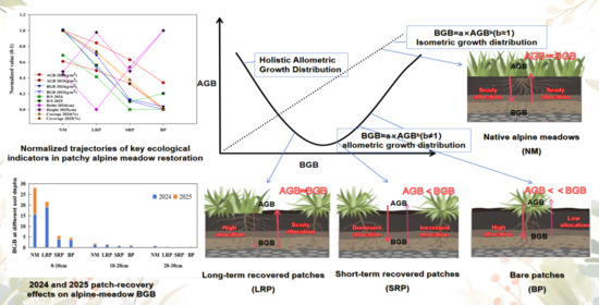
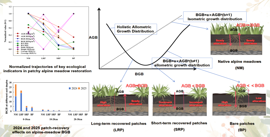
Graphical Abstract

1. Introduction

Alpine meadows are an important part of grassland ecosystems. Because of their extremely high species diversity, water conservation capacity, and carbon sink potential, they play an irreplaceable role in maintaining regional ecological balance and grassland functions [1,2]. However, alpine meadows are generally degraded under interference such as climate change and overgrazing [3], and grassland patchiness has become a typical landscape feature and key driving force in the degradation process [4]. Increasing patchiness in the native mat layer is a precursor to its fragmentation and the expansion of exposed soil. This fragmentation triggers a cascade of ecological effects, including a weakened carbon sink, disruption of the nitrogen cycle, and most critically, immediate biodiversity loss [5,6,7]. This rapid loss contrasts sharply with the slow accrual of biodiversity through long-term speciation processes. Therefore, the recovery process and mechanism of patchy meadows have become the core issue of current alpine ecological restoration research [8].
Biomass is a direct representation of the accumulation of ecosystem materials, and its distribution pattern between aboveground and belowground organs of plants is a core ecological strategy for plants to respond to environmental stress and weigh resource inputs to maintain survival and reproduction [9,10]. This distribution model not only profoundly affects the structure and function of vegetation but is also directly related to key biogeochemical cycle processes such as ecosystem carbon and nitrogen [11]. Currently, the allometric model is widely used to describe the aboveground and belowground biomass relationship in a variety of ecosystems [12,13] and has shown good applicability in biomass estimation of temperate grasslands [14] and desert vegetation [15]. But its universality is being increasingly challenged. Research shows that on environmental gradients such as moisture, plants may switch to an isometric growth strategy [16]. Isometric growth means that different components of an organism (such as aboveground and belowground biomass) grow cooperatively at the same relative rate, and the theoretical value of the scaling exponent in its allometric growth equation is 1 [9,17]. In some natural alpine grasslands, there is also an isometric relationship between aboveground and belowground biomass [18]. In the unique habitat of alpine meadows with extreme low temperatures, strong radiation, and frequent freezing and thawing [19,20], plant allocation strategies may further deviate from the general model, resulting in significant deviations in biomass estimates based on allometric relationships. However, key questions that has been neglected for a long time are the following: How does the biomass allocation pattern of plants change during the dynamic succession sequence of patchy meadows from bareness to complete recovery? Do their aboveground–belowground relationships follow a fixed allometric pattern, or do they undergo fundamental transformations with stages of recovery?
At present, research on the restoration ecology of alpine meadows mostly focuses on changes in community structure or soil physical and chemical properties [21,22,23]. However, there is still a lack of systematic revelation of the distribution rules of aboveground and belowground biomass of alpine meadow vegetation. Clarifying this rule is not only the prerequisite for accurately assessing the carbon sink function during the restoration of alpine meadows but also the basis for understanding the resilience and stability of its ecosystem. To this end, this study took the typical patchy alpine meadow in Henan County, Qinghai Province, as the object and analyzed the changes in plant community biomass and distribution pattern at different recovery stages to measure the following: (1) the dynamic trajectory of the total biomass and aboveground to belowground distribution ratio of plant communities during the natural restoration process; (2) the relationship between aboveground and belowground biomass at different restoration stages, making it clear that it conforms to the allometric or isometric growth model; and (3) how the evolution of biomass allocation strategies correlates with and drives the recovery of key ecosystem functions. By elucidating the evolution of biomass allocation in the restoration continuum, this study not only provides a new quantitative perspective and evaluation index for the restoration effect of degraded alpine meadows, but it also provides a key theoretical basis for predicting the response of the carbon cycle of alpine ecosystems to natural restoration.

2. Materials and Methods

2.1. Overview of the Study Area

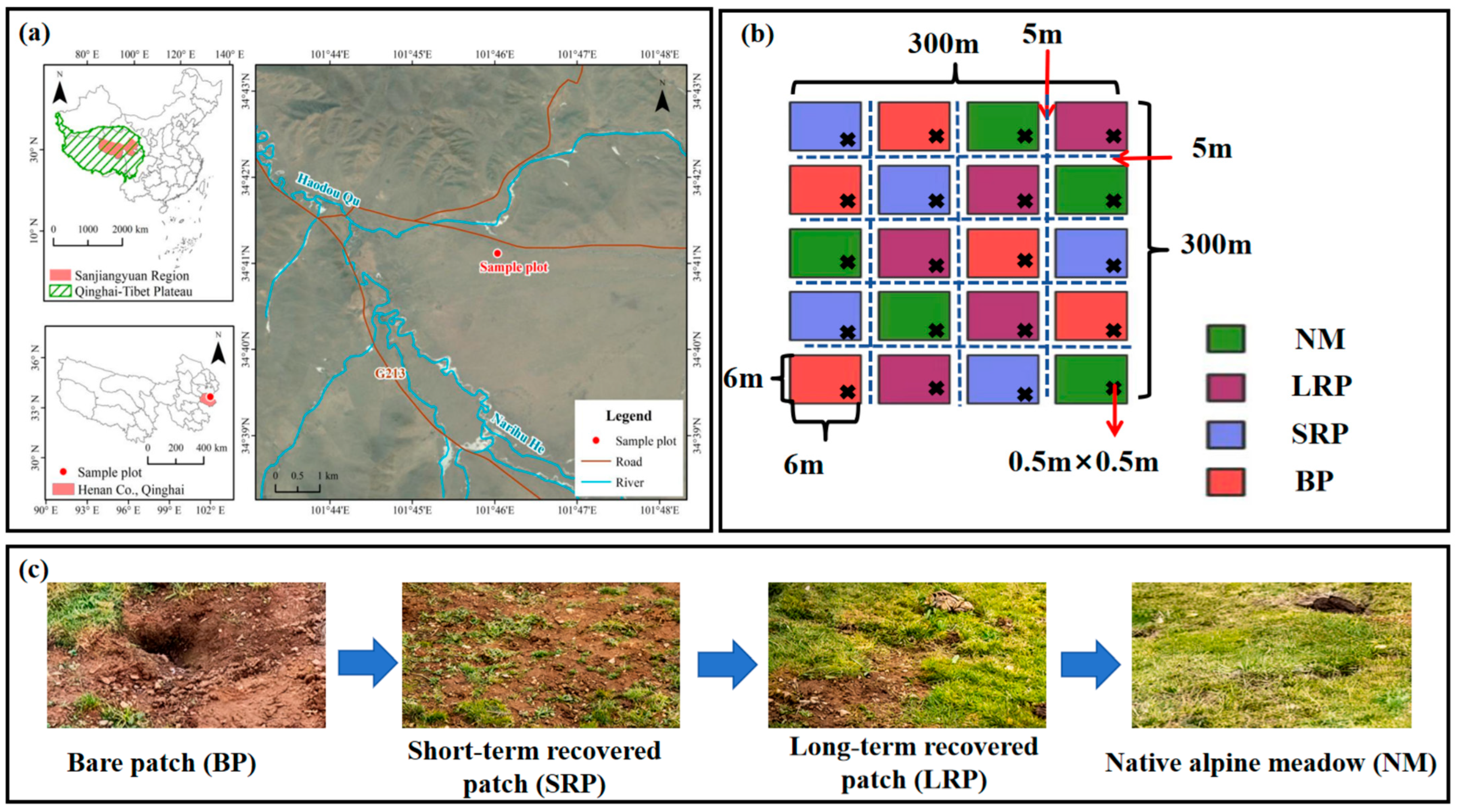
The sample plot of this study is located in Keqihetan, Zexiong Village, Youganning Town, Henan County, Mongolian Autonomous Prefecture, Qinghai Province (Figure 1a). It is under the jurisdiction of the Huangnan Tibetan Autonomous Prefecture and is one of the 14 counties in the “Sanjiangyuan” Nature Reserve in the pastoral area of southern Qinghai. It is an area where moderately degraded alpine meadows are located. Altitude 3610 m, sun-exposed valley bottomlands, slope 3°. This area has a humid climate in the subarctic zone of the plateau, with a long and windy cold season; short summers, a humid and rainy climate. Affected by the plateau monsoon, the seasonal distribution of precipitation is extremely uneven, and most of the annual precipitation is concentrated in summer. The average annual rainfall in 2024 was 0.0011 mm and the average annual temperature was 1.40 °C. In 2025, the average annual rainfall was 0.0012 mm and the average annual temperature was 0.99 °C (Table 1). The plot has flat terrain and stable vegetation community composition.

2.2. Land Use and Management History

All plots in this study were set up in traditional pastures under unified management. In April of 2020 and 2021, efforts were made to exterminate the plateau pika population using the Botulinum Toxin C and carrot as baits. Moderate-intensity seasonal grazing has been implemented for a long time in this area (the stocking rate is about 4.5 yaks·hm−2), and grazing activities are the main land use method. All selected patches were under the same grazing regime to ensure that drivers of the recovery process were comparable. In April of 2020 and 2021, efforts were made to exterminate the plateau pika population using the Botulinum Toxin C and carrot as baits. It is important to note that this study focuses on the “natural recovery” process. No artificial ecological restoration measures (such as seeding, fertilizing, plowing, or engineering fencing) were taken after patch formation and throughout the study period. The restoration of vegetation depends entirely on the soil seed bank, clonal propagation and natural spread of surrounding communities. Therefore, the rules revealed in this study reflect the spontaneous recovery ability of the ecosystem in alpine meadows after disturbances cease under the background of continuous grazing.

2.3. Experimental Design

According to the grassland type map, combined with satellite remote sensing information, and according to the general distribution area of degraded grassland in the Sanjiangyuan area, a sample area was set up in Keqihetan, Zexiong Village, Youganning Town, Henan County Mongolian Autonomous Prefecture. Degraded alpine meadows were categorized into different patch types based on recovery duration: bare patches (BP), short-term recovered patches (SRP), and long-term recovered patches (LRP). Additionally, native alpine meadows (NM) were monitored to represent the pre-degradation ecosystem state. (Figure 1c). The division of meadow patches in this study is based on two core indicators: vegetation type and coverage percentage. All patches are in a state of complete natural recovery without any artificial intervention. The classification follows the methodology established by scholars such as Li Chenyi [8,24,25] and is detailed as follows—BP: Refers to exposed ground formed by physical soil crusts or areas showing clear signs of frequent disturbance by plateau pikas (Ochotona curzoniae). The surface consists of fresh, bare, and loose soil with essentially 0% vegetation coverage. SRP: Areas where plateau pika disturbance ceased 1–2 years prior. These are exposed patches that have undergone approximately 2 years of natural recovery, now accompanied by a small number of successional patches containing annual and biennial forbs. Dominated by plant species such as Elsholtzia densa and Aconitum gymnandrum, with vegetation coverage ranging from 10% to 40%. LRP: Formed through the natural recovery and succession of short-term recovery patches, generally over about 6 years. These patches are accompanied by successional vegetation comprising perennial plant species, such as Elymus nutans and Polygonum macrophyllum. Vegetation coverage ranges from 40% to 70%. NM: Represents healthy alpine meadows that have not experienced disturbance by plateau pikas. This state is equivalent to the stage reached by long-term recovery patches after at least 30 years of natural restoration and succession. Plant species are primarily Kobresia pygmaea and Ajania pallasiana, among others, with vegetation coverage between 70% and 100%. The transition from bare patches to native alpine meadow constitutes a positive natural restoration and succession process. This study was conducted based on the above classification system. The sample area was 300 m × 300 m, and four treatments were set in the sample area, with five replicates for each treatment. The sample plot was selected in a representative area and evenly distributed as far as possible. The plot area was 6 m × 6 m, and there was a buffer zone of 5 m between the plots. A fixed quadrat of 0.5 m × 0.5 m was set in each plot (Figure 1b).

2.4. Sample Collection

The experiment conducted community quadratic surveys at different grassland recovery levels in mid-August in 2024 and 2025, recording species composition and relative coverage (Table 2 and Table 3), and measured the following community characteristic indicators: the height of grassland vegetation, the coverage of each species, and the number of groups. Total coverage, aboveground and belowground biomass were also measured. Use a tape measure to measure the natural height of plants and measure 3 to 5 plants of each plant. When investigating the coverage, record the coverage of all species present in each quadrat on the questionnaire. After the vegetation survey is completed, use the harvesting method to cut all the plants in the quadrat into envelopes and bring them back to the laboratory, dry to constant weight at 80 °C, and measure the dry weight to obtain the aboveground biomass. Use a root drill with a diameter of 8 cm to drill out 0–10, 10–20, and 20–30 cm soil samples from the quadrat where the biomass has been cut, and put them into corresponding Ziplock bags. Then, rinse away the sediment and soil to obtain the plant roots, and bring them back to the laboratory at 80 °C. Dry to constant weight, measure its dry weight, and obtain belowground biomass. The physical and chemical properties of the soil were sent to Sichuan Huabiao Testing Technology Co., Ltd., Chengdu, Sichuan, China. for detection of soil pH, organic matter (SOM), total carbon (TC), total nitrogen (TN), and total phosphorus (TP) (Table 4). The specific measurement method is as follows: The soil pH value is measured using the glass electrode method (soil-to-water ratio 1:2.5), measured in accordance with the NY/T 1121.2-2006 standard [26]. Soil organic matter (SOM) was measured using the potassium dichromate oxidation-external heating capacity method, in accordance with the NY/T 1121.6-2006 standard [27]. Soil total phosphorus (TP) was measured using the sodium hydroxide fusion-molybdenum antimony colorimetric method, based on the LY/T 1232-2015 standard [28]. Soil total nitrogen (TN) and total carbon (TC) were measured using the elemental analyzer method with a Vario EL III elemental analyzer (Elementar Analysensysteme GmbH, Langenselbold, Hesse, Germany). The soil temperature and soil moisture of the sample plots at each restoration stage were measured in situ using the Stevens HydraProbe (Stevens Water Monitoring Systems, Inc., Portland, Oregon, USA), and the data were simultaneously recorded in Table 4.

2.5. Statistical Analysis

SPSS 26.0 software was used to conduct one-way analysis of variance to independently test the effects of different grassland patchy restoration treatments on species diversity and biomass. For indicators that involve comparisons between years (2024 and 2025) and restoration stages (such as vegetation coverage, height, etc.), two-factor analysis of variance is used to test the significance of year (Y), restoration stage (R), and their interaction (Y × R). Before conducting analysis of variance, all dependent variable data were subjected to the Shapiro–Wilk test to assess normality and Levene’s test to assess homogeneity of variances. The data all met the prerequisite assumptions of the parametric test (p > 0.05). Significance test and post hoc comparison: The significance level of analysis of variance was set to α = 0.05. The first step in the analysis is to test the significance of the interaction term (year × recovery stage). If the interaction is not significant (p > 0.05), it indicates that the effect pattern of different recovery stages is consistent between two years. In this case, to simplify the presentation of results and enhance statistical power, we combine the two years of data and focus on the main effects of recovery stage and post hoc comparisons in subsequent analyses. If the interaction is significant (p < 0.05), it indicates that the effect of recovery stages differs between years, and we will report the results separately by year. For those that reach a significant level (p < 0.05), post hoc pairwise comparisons were performed using Duncan’s multiple range test. In the Section 3, groups that are statistically different at the (p < 0.05) level are marked with different lowercase letter superscripts (a, b, c, …). The data were analyzed by SPSS 26.0, and the charts in this section were drawn by software Sigmaplot 15.0 and Microsoft office Excel 2010. The relationship between belowground biomass (BGB) and aboveground biomass (AGB) is usually described using an allometric model. The general form of this model is AGB = a × BGBb, which can be expressed as LogAGB = b × LogBGB + a after logarithmic linearization, where a is a constant and b is the allometric exponent. This study uses standardized principal axis regression to fit and test the parameters of the above log-linear form. According to standard terminology, if the hypothesis test shows that the slope b = 1, it is determined to be isometric growth; if b ≠ 1, it is determined to be allometric growth [29,30]. Isometric growth indicates that aboveground and belowground biomass is allocated in a fixed ratio; allometric growth indicates that the allocation ratio changes with individual size or environment.

3. Results and Analysis

3.1. Dominant Species Composition and Soil Physical–Chemical Properties During Different Patching Restoration Stages

There were significant differences in the plant species composition and relative coverage of alpine meadows at different recovery stages (Table 2 and Table 3). In general, with the recovery of patchy alpine meadows, the community structure shows a successional trend from forbs plants being dominant to an increasing proportion of Cyperaceae plants. Bare patches (BP): The community is in an extremely degraded state. The species composition is simple, the dominant functional groups are not obvious, and the species is dominated by forbs and annual plants. The coverage of Cyperaceae plants is very low (such as Kobresia pygmaea < 1%), while species such as Elsholtzia densa, Cirsium souliei, and Ajania spp. have become common species (Table 1). At the same time, typical pioneer species such as Hedinia tibetica appeared (Table 2). At this stage, the total community coverage is low and the structure is unstable. Short-term recovered patches (SRP): The community structure began to undergo significant reorganization. With the recovery of patchy alpine meadows, forbaceous grasses invaded in large numbers and quickly became the dominant functional group. In particular, the relative coverage of Aconitum gymnandrum jumped to 13% in 2025, becoming the iconic species at this stage (Table 1). The original species are still present, but the cover of sedges such as Kobresia pygmaea has recovered slightly. This indicates that in the early stages of restoration, the direction of community succession points to an unstable transitional stage in which forbs are dominant. Long-term recovered patches (LRP): The community entered a critical transition period. The relative coverage of Kobresia pygmaea has recovered significantly and it has become an important establishing species again, but it has not yet achieved absolute dominance (Table 1 and Table 2). The diversity of forbs reached its peak, with species such as Eriophyton wallichi, Oxytropis spp. and Thalictrum spp. appearing in large numbers, forming a community pattern in which sedges and forbs coexist (Table 2). This stage shows higher species diversity. Native alpine meadows (NM): The community has Kobresia pygmaea of the Cyperaceae family as the absolutely dominant species. Its average relative coverage in two years was as high as 25% and 27%, respectively (Table 2, Table 3). Together with Kobresia humilis and Pedicularis spp., it constitutes a highly stable native vegetation type. The diversity and coverage of forbs decreased significantly, and the community structure was simplified, showing the typical characteristics of being dominated by Cyperaceae plants. In terms of interannual changes, although the composition patterns of dominant species at different recovery stages remained relatively stable between two years, there were certain fluctuations in the relative coverage of each species. Although there are annual fluctuations in the coverage of each species, such as the significant increase in the coverage of Aconitum gymnandrum Maxim. during the SRP stage, the composition of core species and the pattern of dominant functional groups in each recovery stage remained highly consistent between the two years. For example, the NM stage is always dominated by alpine artemisia, while the BP stage always lacks stable dominant species.
As the degree of recovery increases, soil nutrient content (SOM, TN, TC), soil moisture (SWC) and soil temperature (TS) generally show an upward trend, while soil pH values decrease (Table 4). In the bare patches (BP) stage, soil organic matter (SOM) content was at low levels in both years. The total nitrogen (TN) and total carbon (TC) contents are also relatively low. It is worth noting that the soil pH value at this stage was the highest at 8.53 in 2025, which was strongly alkaline. Soil water content (SWC) was the lowest among all stages, while soil temperature (TS) also reached a minimum of 12.10 °C in 2025. Entering the short-term recovered patches (SRP) stage, soil properties begin to differentiate. Compared with the BP stage, the SOM content increased significantly to 45.77 g/kg in 2025, and organic matter began to accumulate in the early stages of vegetation recovery. The TN and TC contents also showed an upward trend. In 2025, TN is 0.30% and TC is 2.86%. However, soil pH continues to rise at 8.43 in 2025. SWC and TS are similar to the BP stage. In the long-term recovered patches (LRP) stage, the soil nutrient accumulation trend is more obvious. The SOM and TC contents continue to increase. In 2025, SOM is 40.47 g/kg, TC is 2.78%, and TN content is 0.28%, which is also higher than the BP stage. A key change is that soil pH begins to decline from its peak in the SRP stage but is still significantly higher than in the NM stage. SWC improved slightly but not significantly, while TS continued to show a warming trend. Finally, in the native alpine meadows (NM) stage, the soil presents optimal fertility conditions and the most stable environment. The soil organic matter (SOM) content is significantly higher than in other stages, specifically reaching a peak of 57.65 g/kg in 2024. The total nitrogen (TN) and total carbon (TC) contents also reached the highest levels. The lowest soil pH in the NM stage is 7.81–7.93. Soil moisture content (SWC) during this phase will be at a maximum of 0.35% in 2024. Diurnal variation in soil temperature (TS) is large, but the average temperature is moderate. Interannual changes show that multiple indicators in all recovery stages show certain fluctuations in 2025. The TP (total phosphorus) content of each stage generally increased in 2025, while TS generally decreased. However, the overall ranking pattern of soil properties between the restoration stages remained stable over the two years: SOM, TN, and TC were always the highest in the NM stage, and pH was always the lowest; SWC was always the lowest in the BP stage.

3.2. Effects of Different Restoration Stages of Patching on Alpine Meadow Coverage and Height

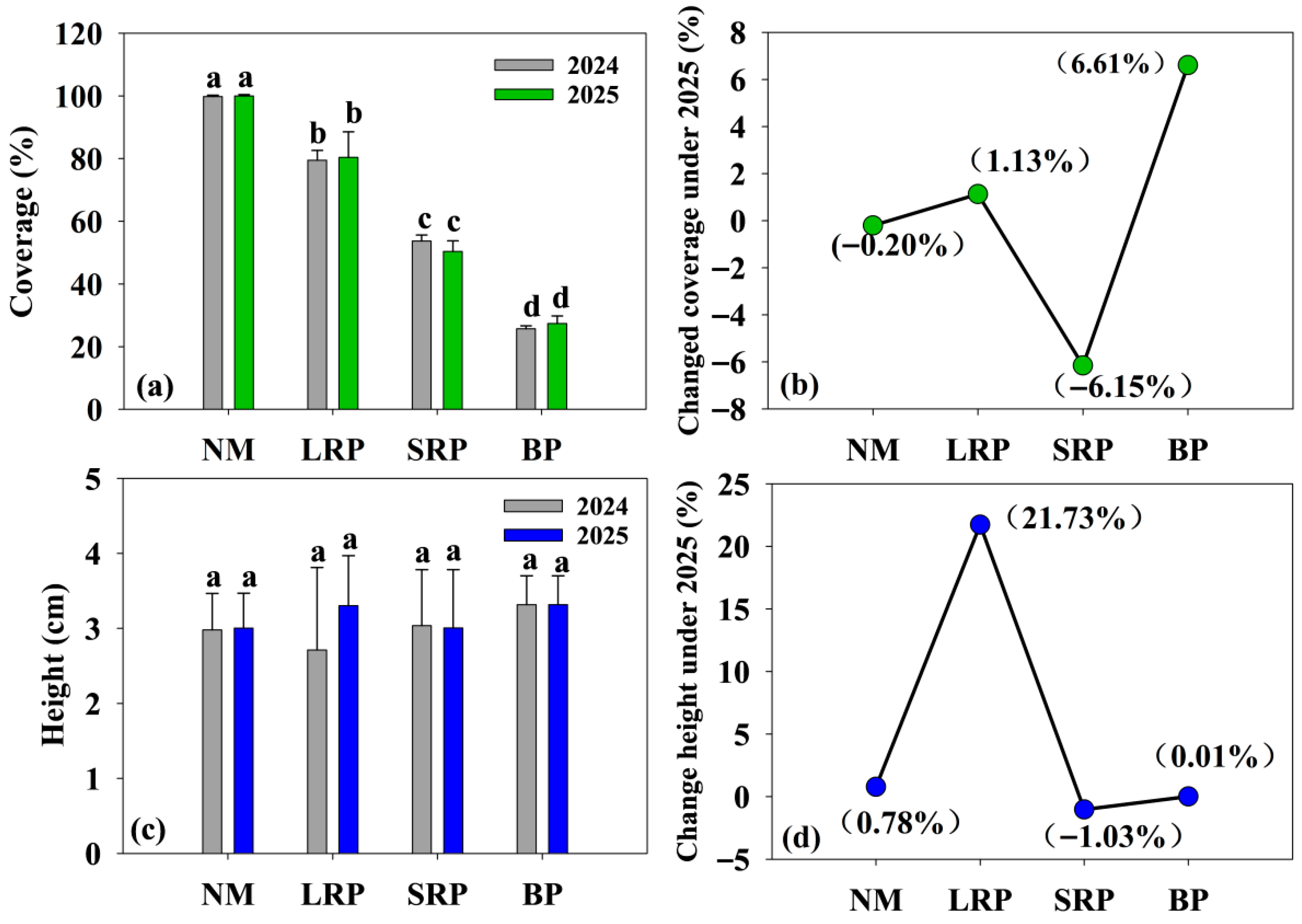
We found that the recovery stage had a highly significant impact on community coverage (p < 0.01), and the interannual and interannual interaction effects with recovery stage had no impact on community coverage (Table 5). This suggests that the pattern of effects of the recovery phase on cover is stable and consistent across years. Therefore, we combined the two years of data to analyze the main effect of recovery stage (R) on cover. However, the interaction effects between years, recovery stages, and between years and recovery stages had no effect on community height (Table 5). This shows that during this study, vegetation height did not show statistically significant differences at different recovery stages and between different years. Table 6 shows the changes in vegetation coverage and height at different restoration stages and their difference test results. There were extremely significant differences in coverage between different recovery stages (p < 0.001). The highest coverage of NM was 100.0%, which was significantly higher than that of all other stages. As the recovery stage progressed, the vegetation coverage showed a significant and regular downward trend, in the order of NM > LRP > SRP > BP. For vegetation height, although the observed values at different restoration stages fluctuated slightly, no statistically significant differences were found (p > 0.05), and the average height at each stage remained between 3.0 and 3.3 cm.
In different recovery stages, the community coverage in the two years was NM > LRP > SRP > BP. In 2025, compared with NM, LRP increased from 80.4% to 100%, an increase of 19.6%; SRP increased from 50.4% to 100%, an increase of 49.6%; and BP increased from 27.4% to 100%, an increase of 72.6% (Figure 2a). From 2024 to 2025, the relative change in community coverage in different restoration stages showed that LRP had the highest change, SRP had lower change, NM was close to 0, and BP had a slight change (Figure 2b). The community height in 2024 was BP > CK > LRP > SRP. The community height in 2025 was LRP > BP > SRP > CK (Figure 2c). From 2024 to 2025, the relative changes in community height in different restoration stages showed that LRP changed the most, NM changed less, BP was close to 0, and SRP decreased slightly (Figure 2d).

3.3. Effects of Different Restoration Stages of Patching on Aboveground and Belowground Biomass of Alpine Meadow Community

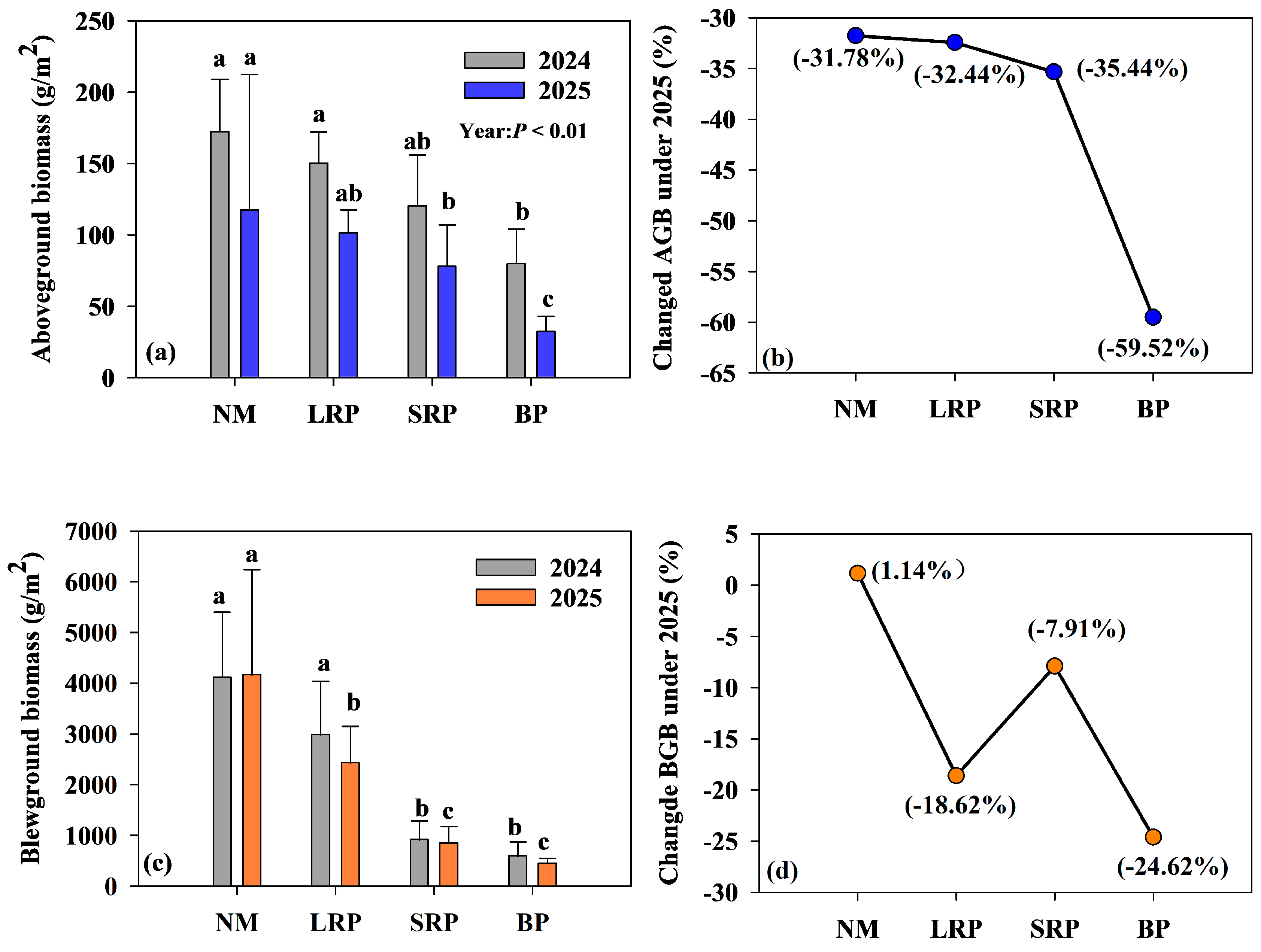
We found that for aboveground biomass (AGB), interannual variation and recovery stage had a significant impact on average annual biomass (AGB) (p < 0.01). The interaction between interannual variation and recovery stage had no significant effect on AGB (Table 7). This shows that despite differences in overall AGB levels between the two years, the pattern of effects of different recovery stages on AGB (i.e., the relative differences between treatments) is stable between the two years. Therefore, we combined the two years of data to analyze the main effect of the recovery stage (R) on AGB. For belowground biomass (BGB), the interaction between interannual variability and recovery stage had no significant effect on BGB. The recovery phase had a significant effect on BGB (p < 0.01) (Table 7). This also shows that the impact of the recovery stage on BGB is consistent between different years, so we also merged the two years of data to analyze the main effect of the recovery stage (R). Table 8 shows the changes in aboveground biomass and belowground biomass of vegetation at different restoration stages and their difference test results. There are extremely significant differences in AGB between different recovery stages (p < 0.001). There is no significant difference between NM, LRP and SRP, while BP is significantly lower than the first three. The difference in BGB is extremely significant (p < 0.001). NM was significantly higher than other stages, followed by LRP, and the difference between SRP and BP was not significant, indicating that belowground biomass showed a significant increasing trend with the continuous recovery of the patchy alpine meadow.
The community AGB in 2024 and 2025 was NM > LRP > SRP > BP (Figure 3a). In 2025, the lowest AGB of BP was 32.31 g/m2, which was significantly lower than NM by 72.51%; LRP was significantly higher than NM by 13.63%, and SRP was significantly lower than NM by 33.73% (Figure 3a). From the relative changes of BGB in each recovery stage from 2024 to 2025, NM has the smallest increase and an upward trend, while LRP, SPR and BP have a downward trend. (Figure 3d).
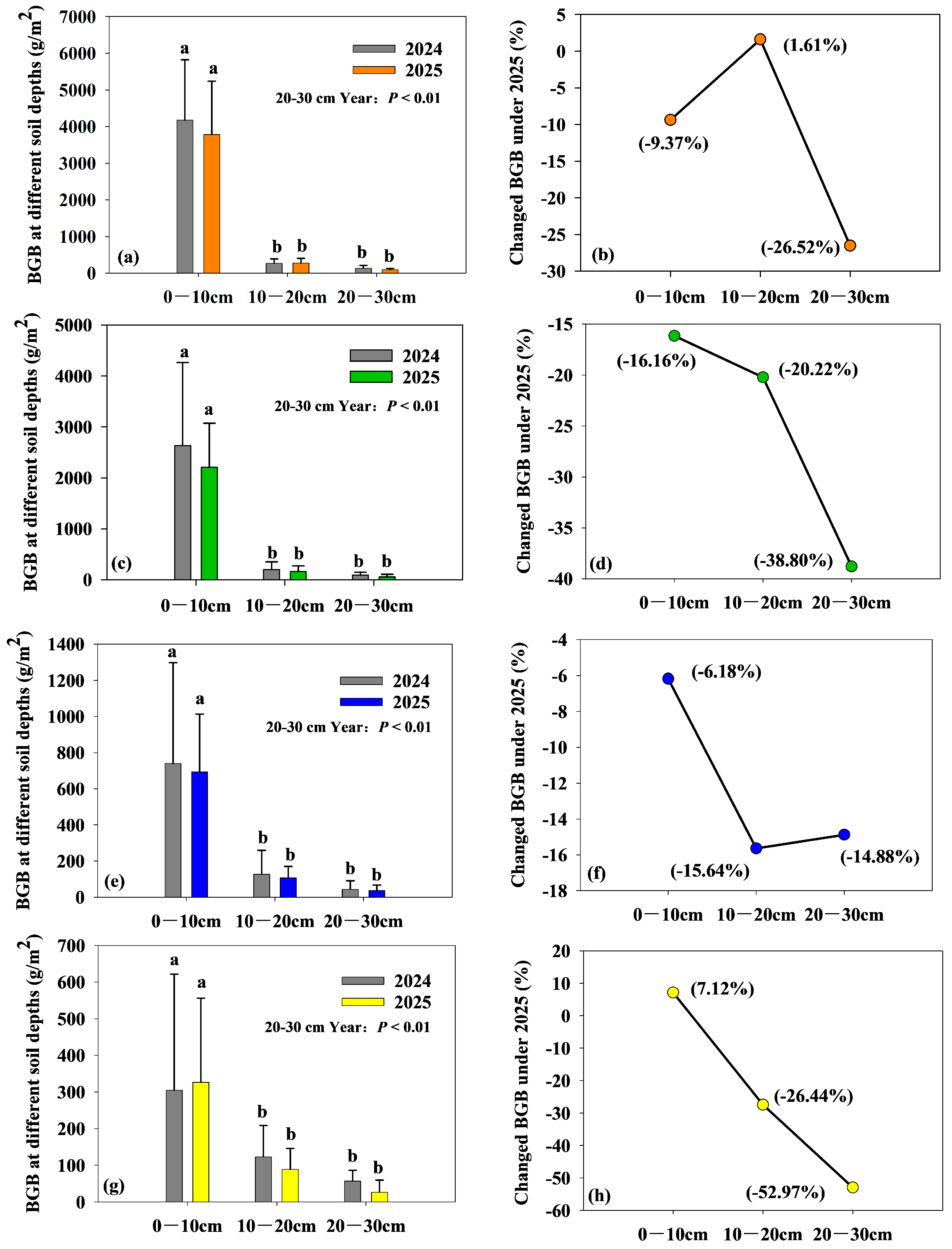
In order to further explore the effects of different restoration stages on BGB at different soil depths in alpine meadow communities, we also measured BGB from 10, 20 and 30 cm deep soil. The recovery stage had a very significant effect on the BGB of 0–10 cm, 10–20 cm and 20–30 cm soil (p < 0.01). The interannual and the interaction between interannual and recovery stages had no effect on the BGB of 10–20 cm and 20–30 cm and soil, while the interannual had a very significant effect on the BGB of 0–10 cm soil (p < 0.01) (Table 9). For the 0–10 cm, 10–20 cm and 20–30 cm soil layers, the interaction between year and recovery stage (Y × R) was not significant (p values were 0.779, 0.865 and 0.606 respectively). This shows that the pattern of effects of the restoration phase on belowground biomass remains consistent between 2024 and 2025, regardless of year. Therefore, we subsequently combined the two years of data to analyze the main effect of recovery stage (R) in each soil layer. Table 10 shows the changes in different soil layers at different restoration stages and their difference test results. Overall, the belowground biomass content in each soil layer showed a very significant downward trend as the degree of recovery weakened (p < 0.001). As the soil layer deepens, NM is significantly higher than in other stages, followed by LRP, and the difference between SRP and BP is not significant, indicating that belowground biomass shows an obvious downward trend with the weakening of recovery degree.
During 2024–2025, the relative changes in BGB in different restoration stages showed obvious soil layer differences: NM remained stable at the depths of 0–10 cm and 10–20 cm, and only a large fluctuation occurred in the 20–30 cm layer (Figure 4b); LRP and SRP showed negative growth in the three layers of 0–10 cm, 10–20 cm and 20–30 cm (Figure 4d,f). The 0–10 cm BGB of BP increased slightly, while the 10–20 cm and 20–30 cm layers showed negative growth (Figure 4h).

3.4. Effects of Different Restoration Stages of Patching on Root–Shoot Ratio of Alpine Meadow Community

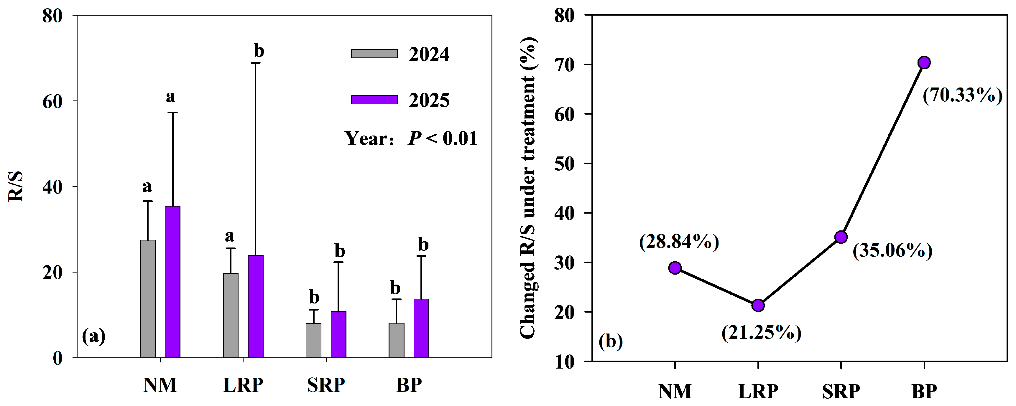
In this study, interannual and recovery stage had extremely significant effects on R/S (p < 0.01), while the interaction effect between interannual and recovery stage had no effect on R/S (Table 11). The results of the two-way ANOVA on the root-to-shoot ratio (R/S) of alpine meadow patches in 2024 and 2025 are shown in Table 11. The analysis shows that the interaction between year and recovery stage (Y × R) is not significant (F = 0.274, p = 0.844). This shows that the pattern of effects of different recovery stages on root-to-shoot ratio is consistent between the two years. Therefore, we combined the data from 2024 and 2025 to analyze the main effect of the recovery stage (R). Table 12 shows the changes in R/S at different recovery stages and its difference test results. The difference in R/S is extremely significant (p < 0.001). NM was significantly higher than other stages, followed by LRP, and the difference between SRP and BP was not significant, indicating that R/S showed a significant increasing trend with the continuous recovery of patchy alpine meadow.
The R/S in 2024 and 2025 are NM > LRP > BP > SRP. Compared with LRP, R/S and NM in 2025 were reduced by 34.34%, 70.41% and 62.33%, respectively (Figure 5a). Judging from the relative changes in R/S at different recovery stages from 2024 to 2025, BP has the highest change, while the changes in NM, LRP, and SRP are smaller than BP. R/S in different recovery stages has an increasing trend (Figure 5b).

3.5. Relationship Between Aboveground Biomass and Belowground Biomass of Community

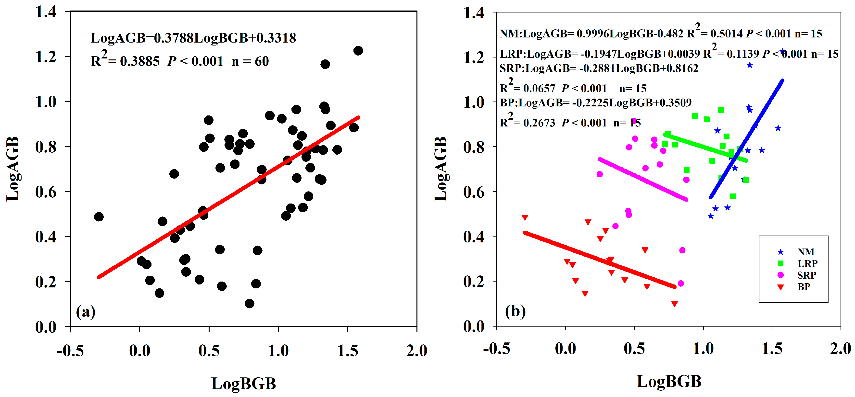
In order to further explore the relationship between different recovery stages, two allocation hypotheses were tested by testing the plant biomass allocation in different recovery stages. It was observed that there was an allometric relationship between the overall AGB and BGB distribution (Figure 6a). There was a significant correlation between AGB and BGB (p < 0.001, Figure 6a). The distribution of AGB and BGB in NM belongs to the isometric growth relationship (Figure 6b), while the distribution of AGB and BGB in other recovery stages belongs to the allometric growth relationship (Figure 6b). There was a significant positive correlation between AGB and BGB in NM, while there was a significant negative correlation between AGB and BGB in LRP, SPR and BP (p < 0.001, Figure 6b).

4. Discussions

4.1. Dynamics of Plant–Soil Interactions Across Restoration Stages

During the restoration process of patchy alpine meadows, the community species composition showed a trend of transformation from forbaceous grasses to sedge plants. This transformation mechanism mainly includes the following two aspects: On the one hand, rodents such as plateau pikas (Ochotona curzoniae) prefer to dig burrows in forbaceous grass patches. With the gradual recovery of alpine meadows, sedge plants can fully grow clonally and achieve community canopy closure, thus compressing the living space of forbible grasses [31]. On the other hand, the recovery of alpine meadows is accompanied by the gradual recovery of soil nitrogen and phosphorus contents, but there are differences in the spatiotemporal utilization strategies of nutrients by plants of different functional groups: sedge plants (such as Kobresia pygmaea) retain nutrients in the surface root mat through a developed belowground rhizome system, while forbs are mostly annual plants (such as Pedicularis spp.), whose renewal relies on the surface soil seed bank and rapid germination strategies and is more sensitive to changes in soil nutrients [32]. As the restoration process progresses, the nutrient competitiveness of the sedge family gradually increases, while the forbic grasses are at a competitive disadvantage. This study also found that as the restoration process progresses, soil nutrient content (SOM, TN, TC), soil moisture (SWC) and soil temperature (TS) generally show an upward trend, while soil pH values decrease. The reasons can be summarized as the following three points: (1) The root systems of Ranunculaceae and leguminous plants (such as Aconitum gymnandrum and Oxytropis spp.) that appear during the restoration process can further enrich the nitrogen and phosphorus input from the litter and biological nitrogen fixation and quickly transport them to the leaves. The leaf N and P The concentration is significantly higher than that of Cyperaceae, so they in turn feed back more active nitrogen and phosphorus to the soil, forming a positive nutrient amplification effect, thereby occupying and holding canopy gaps faster within this self-fertilization window [33], increasing the nitrogen and phosphorus content of the soil. (2) The continuous accumulation of soil organic matter (SOM) and total carbon (TC) promotes nitrification and organic acid secretion, leading to a decrease in soil pH [34]. (3) The increase in alpine meadow vegetation coverage increases soil water content (SWC) and soil temperature (TS), which helps to extend the community photosynthesis cycle. At the same time, it makes meadow plant seeds more accessible to light spots, reducing shading stress in the seedling stage, thus promoting species replacement within functional groups and forming a richer grass population [35].

4.2. Effects of Different Restoration Stages of Patching on Coverage and Height of Alpine Meadow

Grassland coverage and height are important indicators to measure grassland productivity [36]. This study observed that the coverage of NM is the largest and that of BP is the smallest. This is the same as the previous research results [37] in the Patagonian grassland in northwest Argentina. The reason for the minimum community coverage in BP is that although the digging activities of plateau rodents (such as Ochotona curzoniae) do not directly change the soil texture, they destroy the stability of plant–soil feedback by destroying plant root connections, removing aboveground biomass, and constructing cave micro-topography [38], resulting in a reduction in aboveground biomass, thereby reducing community coverage. In contrast, the high coverage state of NM reveals the central role of clonal growth in maintaining community stability [39]. Dominant species that grow clonally from rhizomes or tillers (such as Kobresia humilis and Kobresia humilis) use physiological integration to efficiently utilize resources and quickly fill gaps, forming an anti-interference space occupation strategy. From 2024 to 2025, community coverage LRP and SRP changed positively, BP changed negatively, and NM was almost unchanged at different recovery stages. The positive changes in LRP benefit from the positive feedback loop of soil structure–vegetation: the dense root system of perennial plants (such as Pleurospermum spp.and Gentiana spp.) consolidates the soil [40], improves the microenvironment, and thus promotes further expansion of vegetation. This is essentially an ecosystem self-reinforcing process. The positive changes in SRP more reflect the role of the microenvironment modification function of the mature plant (such as shading, erosion reduction) in promoting early settlement [41]. Comparison between the two shows that the early stage of recovery relies on the improvement of the physical environment, while the middle and later stages rely on self-sustainability driven by biological processes. The negative change in BP is because the vegetation coverage of BP is small and is susceptible to wind erosion, which causes the content of soil organic matter to decrease, and the coverage of BP shows negative changes [42]. If the aboveground biomass of NM is not affected by external forces such as harvesting or fire, nitrogen will enter the topsoil in the form of litter and be mineralized year by year, thereby maintaining available nitrogen at a low but stable level [43], which is not enough to allow rapid expansion of the community but also avoids continued degradation, allowing the coverage of NM to remain basically unchanged.
Changes in the average height of the community sensitively reflect the life history strategies of dominant plants and their responses to environmental conditions. BP’s height peak in 2024 is in sharp contrast to its low cover state. During the monitoring year, BP reached the highest value in that year due to the rapid uplift of pioneer or noxious weeds [44]. The LRP will be the highest in 2025, indicating that the community has entered a more mature stage. In long-term restored patches, due to the maturity of the community and the increase in plant height of dominant species [45], the average height of the community is passively raised. From 2024 to 2025, community height NM and LRP have positive changes at different recovery stages, SRP has small negative changes, and BP is almost unchanged. This may occur because NM plants will preferentially invest all photosynthetic products in the extended growth of vegetative organs (stems, leaves) to quickly occupy light resources, which is manifested as an increase in plant height [46]. The biggest change in height of LRP is because after 10–20 years of restoration, the accumulation of carbon, nitrogen, and phosphorus in the litter-root system was significantly higher than that in degraded patches, the nitrogen supply changed from limited to sufficient, and plants invested more resources in stem and leaf elongation instead of root defense [25], which promoted the increase in vegetation height. Most of the plants (such as Aconitum gymnandrum Maxim. and Elsholtzia densa Benth.) in SRP are one or two years old. Annual herbs will die after flowering and fruiting within one growing season. They will be replaced by perennial low species in subsequent succession stages, so there will be a negative growth in height [47]. BP shows that the vegetation coverage is low, and most of it is bare alpine meadow soil, resulting in a weak ability of the surface to reduce wind speed. The wind erosion process can blow away the roots of newly germinated seedlings in BP or cause the root neck to be exposed, making their survival rate close to zero [48], so the plant height remains basically unchanged.

4.3. Biomass Accumulation Patterns and Their Implications for Ecosystem Function Recovery

This study shows that during the natural recovery process of alpine meadows, the total biomass of plant communities and the biomass of aboveground and belowground components increased significantly with the recovery process, which is consistent with the general law of recovery of degraded ecosystems [49,50]. This may be because vegetation restoration reduces surface exposure and reduces soil water evaporation, allowing water to be stored in the soil for a long time for plants to absorb and utilize, resulting in a gradual increase in the aboveground and belowground biomass of the community [51]. Interannual comparisons revealed differences in patterns of aboveground biomass change during different recovery stages. Aboveground biomass in exposed patches declined in 2025, which may be related to interannual fluctuations in pioneer plant (such as Elsholtzia densa Benth. and Ajuga lupulina Maxim.) communities. Species composition data show that this stage is dominated by mono- and biennial herbs with short life histories, and their biomass is highly susceptible to interannual climate fluctuations (such as precipitation at the beginning of the growing season) [52]. In contrast, native meadows are dominated by perennial grasses (such as Kobresia humilis and Kobresia humilis), the community structure is stable, and their aboveground biomass remains relatively stable between years [53].
Compared with the aboveground part, the interannual changes in belowground biomass are more complex and show obvious differences with recovery stages. After long-term natural selection, the plant community of native meadows is mainly composed of perennial plants (such as Kobresia humilis and Kobresia humilis), which are relatively stable and have slow interannual turnover; BGB can accumulate year by year [54]. Therefore, the N has the smallest increase but maintains an upward trend. Whether it is long-term or short-term recovery, it starts with bare patches. Exposed patches (areas disturbed by Ochotona curzoniae) have seriously damaged the original soil structure, and these damaged soil environments always restrict the recovery process [55]. Therefore, LRP, SPR and BP changed greatly and showed an overall decrease. This study found that the belowground biomass gradually decreased with the deepening of the soil layer.
This study found that belowground biomass gradually decreased as the soil layer deepened. This is consistent with previous research results on belowground biomass [56]. This occurs because the majority of belowground biomass (BGB) is distributed in the surface soil (such as 0–10 cm) [57]. Most organic matter and nutrients are stored in the soil surface, and plant roots are mainly distributed in the surface soil to obtain more resources to meet growth needs [58]. As the soil depth increases, the nutrient and organic matter content in the soil gradually decreases, resulting in a decrease in belowground biomass. We conducted an in-depth analysis of interannual vertical changes in belowground biomass (BGB) during different restoration stages and discovered stage-specific dynamic patterns. The BGB of LRP, SRP and BP in different soil layers in 2025 showed a downward trend compared with 2024. Among them, LRP in the 0–10 cm soil layer decreased by 6.18%, while BP increased by 7.12%. SRP in the 20–30 cm soil layer decreased by 14.88%, which was slightly lower than the 15.64% in the 10–20 cm soil layer. This is because carbon saturation in the surface layer of LRP increases biological C/N, and nitrogen fixation causes nitrogen deficit in the rhizosphere. In order to reduce nitrogen loss, plants actively reduce the density of fine roots in this layer [59], resulting in a decrease in BGB in the surface layer. The dominant species of BP is annual grass (such as Elsholtzia densa Benth.), and its life history strategy is to invest all limited photosynthetic carbon into the 0–10 cm fibrous root system in order to quickly absorb water and complete the life cycle in short-term rainfall pulses [60], resulting in an increase in BGB in the surface layer. The SRP community is dominated by one- and two-year herbaceous plants (such as Aconitum gymnandrum Maxim. and Elsholtzia densa Benth.). In order to compete for aboveground resources, plants preferentially invest limited carbon in the aboveground parts, resulting in a general decrease in root carbon allocation and becoming a common starting point for biomass decline in the entire soil layer [61], resulting in the smallest BGB in the middle layer.

4.4. Adaptive Strategies of Alpine Meadow Plants to Patchy Habitats: Insights from Root–Shoot Ratio

Root-to-shoot ratio is the core variable connecting carbon and nitrogen absorption and plant structure evolution [62]. Because there are many factors affecting the root–shoot ratio (R/S), the data of grassland root–shoot ratio in different regions are inconsistent [63,64]. We found that the root–shoot ratio of the community increased with restoration, but BP was larger than SRP. In the short-term restoration process, the vegetation has just begun to grow, and the aboveground part needs to grow rapidly to obtain more light resources, thus gaining an advantage in the competition [65]. Therefore, plants allocate more resources to the aboveground part, resulting in a smaller root–shoot ratio. BP are visual manifestations of severe ecosystem degradation, usually accompanied by severe abiotic stresses such as flooding, strong wind erosion, or sustained drought [66]. These stress factors directly destroy vegetation and soil structure, creating an environment that is unfavorable for plant settlement and growth. In this study, BP showed a significantly larger root-to-shoot ratio. This observed statistical pattern more likely reflects two mutually exclusive ecological processes: (1) The results of environmental filtering and community construction: The harsh stress environment acts as a strong filter [67], eliminating species with shallow root systems or poor tolerance, allowing species that can survive or successfully colonize at this stage and have a natural tendency to invest larger root biomass to dominate the community [68]. (2) Potential plastic response at the individual level: Individual plants may allocate more resources to the root system to enhance their ability to colonize and survive in stressful environments [69,70]. The R/S of different recovery stages from 2024 to 2025 is increasing. It may be because in the early stage of recovery, more resources are allocated to the aboveground part to quickly occupy space and compete for light [71]. Over time, species began to increase their large belowground roots to enhance their long-term viability in water and nutrient competition [72]. This change will inevitably lead to an increase in the overall root–shoot ratio of the community.

4.5. Correlation Growth Relationship Between Aboveground and Belowground Biomass

We found that the aboveground and belowground biomass of the alpine meadow generally conformed to the allometric growth model, but the native meadow conformed to the isometric growth model, while other patch types conformed to the allometric growth model. Therefore, using the allometric growth model to estimate the belowground biomass of grassland will reduce the damage to the grassland system to a certain extent. Studies have found that the addition or change in N enhances the distribution of aboveground biomass, resulting in allometric growth [19]. However, some scholars have shown that the distribution of aboveground and belowground biomass in grasslands showed an isometric growth relationship [73,74]. There are many reasons for these differences, such as the insufficient number of grassland sampling points and the change in climate characteristics and topography in the study area, which may affect the growth relationship of grassland biomass. As the total biomass of plant communities increases, relatively more biomass is allocated to belowground organs, which is consistent with the results [75] based on alpine grasslands on the Qinghai–Tibet Plateau. Plants usually allocate more biomass to the most restricted structures and functions in their habitats [76,77].
The native meadow conforming to the isometric growth model may be because of the following: (1) As a mature ecosystem, the native meadow has a highly coordinated soil nutrient cycle (such as carbon–nitrogen ratio). This coordinated nutrient cycle can provide a stable nutrient supply for plants, allowing plants to distribute biomass more evenly during growth [78]. (2) The native meadow ecosystem has high stability and self-regulation ability. In the absence of external interference, various ecological processes within the ecosystem can remain relatively stable, providing good environmental conditions for the constant growth of plants [79]. The possible reasons for the allometric relationship in other recovery stages are as follows: (1) Plants with short-term recovery patches may be in the early stage of recovery and need to quickly adapt to environmental changes. Through allometric growth, plants can adjust their biomass allocation more flexibly to cope with environmental stress [80]. (2) The ecosystem of long-term restoration patches is relatively stable, and plant growth is regulated by a variety of ecological processes. For example, the coordination of soil nutrient cycling and microbial communities allows plants to allocate biomass more evenly, but some functional parts (such as stems) may grow faster due to the need for support and transport functions [81]. (3) The distribution of soil nutrients in the bare patch is uneven, and the biomass allocation of plants will be adjusted according to the availability of nutrients during the growth process [82]. This inhomogeneity may lead to differences in the growth rate of different parts of the plant, resulting in allometric growth.
The alpine meadow AGB and BGB generally conform to the allometric growth model, but NM conforms to the isometric growth model. This difference is caused by the following: (1) The investment proportions of the three types of functional plants, grasses, sedges and weeds, in stems, leaves and roots are significantly different. Annual species invest more biomass into stems and reproductive organs, while perennial species strengthen root system construction [83]. This differential configuration determines the difference in intercept and slope of the allometric relationship. (2) In the early stages of recovery, the community is dominated by a few pioneer species, which have a single survival strategy and often respond to stressful environments by investing heavily in root systems (a relatively high R/S ratio), resulting in strong allometric growth. As restoration proceeds, species diversity increases and ecological niches diverge. Some species mainly invest aboveground, while others invest mainly belowground [84,85]. This complementation and integration of functional traits make the biomass allocation at the community level tend to be a more balanced portfolio, thus exhibiting isometric growth. This is consistent with community function being dominated by traits of dominant species [86]. (3) Recovery is essentially a process of environmental screening of pressure changes. In the early days, stress-intolerant species were filtered out through harsh environments such as drought, erosion, and low temperature, and species with deep roots and high R/S were screened out [67,87]. At the climax stage, abiotic stresses ease and biotic interactions (such as competition and promotion) become the main screening force [88]. Competition for light resources favors tall or fast aboveground growing species, thereby changing the biomass distribution pattern of the entire community away from earlier allometric growth patterns.
The AGB and BGB of NM is positively correlated, possibly because the growth of aboveground and belowground parts of plants are coordinated with each other. The aboveground part produces organic matter through photosynthesis to provide energy and nutrients to the belowground part, while the belowground part absorbs water and nutrients to support the growth of the aboveground part [89]. Photosynthesis in the aboveground part provides energy and organic matter to the belowground part, while the roots in the belowground part absorb water and nutrients to support the growth of the aboveground part [90]. This coordination creates a positive correlation between AGB and BGB, that is, when AGB increases, BGB will also increase accordingly. The AGB and BGB of LRP, short SRP and BP are negatively correlated, possibly because of the following: (1) As the recovery time prolongs, the main function of the ecosystem may shift from rapid growth and resource acquisition to resource maintenance and enhanced stability. This functional shift may cause plants to allocate more resources to belowground parts to enhance soil structure and nutrient cycling capabilities, thereby reducing aboveground biomass accumulation [91]. (2) During the restoration process, the plant community structure gradually changes [90], and the replacement of certain plant functional groups (such as grasses and sedges) may lead to changes in the distribution of AGB and BGB. (3) During the recovery process of BP, the growth strategies of plants will change. In the early stage, plants will prioritize the development of belowground parts to establish a stable root system to provide support for subsequent growth of aboveground parts [92]. This staged development strategy will lead to a negative correlation between AGB and BGB.
The transition from allometric growth to isometric growth is not caused by a single factor but is the inevitable result of the joint action of the community structure from simple to complex and the dominant screening factors from abiotic to biotic during the restoration and succession of alpine meadows. This distribution strategy turning point revealed in this study provides a potential quantitative indicator for assessing whether the alpine meadow ecosystem has truly returned to a state of structural stability and functional balance.

5. Conclusions

In summary, this study took the patchy alpine meadow on the Qinghai–Tibet Plateau as the object and set up three recovery stages: bare patches (BP), short-term recovery patches (SRP), and long-term recovery patches (LRP). Using the native meadow (NM) as the control, we simultaneously measured aboveground and belowground biomass, root-to-shoot ratio (R/S), and vegetation coverage and height. The results showed that with the advancement of alpine meadow patchy restoration process, both the aboveground and belowground biomass of the community showed a significant increasing trend, and the belowground biomass showed an obvious decreasing pattern with the increase in soil depth. The root-to-shoot ratio (R/S) shows a dynamic change characteristic of first increasing and then decreasing. This study found for the first time that meadow patches in the restoration stage all followed an allometric growth distribution strategy, and biomass distribution was significantly biased toward the belowground part, while native meadows maintained an isometric growth distribution pattern. During the restoration process, the vegetation was dominated by pioneer species (such as Elsholtzia densa Benth. and Ajuga lupulina Maxim.) and gradually transitioned to perennial grasses (such as Kobresia humilis and Kobresia humilis). The succession of species composition not only drives biomass accumulation but also reflects the process of gradual recovery of ecosystem structure and function. It provides an important theoretical basis for the ecological restoration practice of degraded meadows. Based on the research conclusions, the restoration of alpine meadows should follow the core principle of “roots first, leaves later”. The nutrient supply of belowground roots can be strengthened through moderate fertilization, and fencing measures can be used to eliminate interference from humans and animals, ensuring the effective implementation of belowground priority growth strategies, thereby accelerating the succession process of degraded meadows to native top communities. It should be noted that the observation period of this study is only two years, and the long-term stability of the biomass distribution pattern and its regulatory mechanism still need to be further verified through long-term positioning monitoring in order to provide more systematic theoretical support for the precise restoration and scientific management of alpine meadows.

Author Contributions

Conceptualization, Y.J. and C.L.; Methodology, Y.J. and C.L.; Software, Y.J., T.D. and J.H.; Validation, Y.J. and C.L.; Formal Analysis, Y.J. and J.H.; Investigation, Y.J., C.L., T.D. and J.H.; Resources, C.L., Y.Y. and X.L.; Data Curation, Y.J., T.D. and J.H.; Writing—Original Draft, Y.J.; Writing—Review and Editing, C.L.; Visualization, Y.J. and T.D.; Supervision, C.L. and Y.Y.; Project Administration, C.L. and X.L.; Funding Acquisition, C.L. and X.L. All authors have read and agreed to the published version of the manuscript.

Funding

This research was funded by National Natural Science Foundation of China, grant number 32160289. Project supported by the Independent Project of the National Key Laboratory of Sanjiangyuan Ecology and Plateau Agriculture and Animal Husbandry, Qinghai University, grant number 2022-ZZ-03. And project supported by the Independent Project of the Ecosystem Succession and Management Direction, Ecology Discipline of World-Class grant number 2025-ZZ-05.

Data Availability Statement

The raw data supporting the conclusions of this article will be made available by the authors on request.

Conflicts of Interest

The authors declare no conflict of interest.

References

  1. Körner, C.; Kèorner, C. Alpine Plant Life: Functional Plant Ecology of High Mountain Ecosystems; Springer: Berlin/Heidelberg, Germany, 1999. [Google Scholar] [CrossRef]
  2. Nagy, L.; Grabherr, G. The Biology of Alpine Habitats; Oxford University Press: New York, NY, USA, 2009. [Google Scholar] [CrossRef]
  3. Sun, J.; Zhang, Z.; Dong, S. Adaptive management of alpine grassland ecosystem in Qinghai-Tibet Plateau. Pratacultural Sci. 2019, 36, 933–938. [Google Scholar] [CrossRef]
  4. Li, J.; Shao, X.; Huang, D.; Shang, J.; Liu, K.; Zhang, Q.; Yang, X.; Li, H.; He, Y. The addition of organic carbon and nitrogen accelerates the restoration of soil system of degraded alpine grassland in Qinghai-Tibet Plateau. Ecol. Eng. 2020, 158, 106084. [Google Scholar] [CrossRef]
  5. Li, C.; Li, X.; Yang, Y.; Shi, Y.; Zhang, J. Comparative responses of carbon flux components in recovering bare patches of degraded alpine meadow in the Source Zone of the Yellow River. Sci. Total Environ. 2024, 908, 168343. [Google Scholar] [CrossRef] [PubMed]
  6. Jin, P.; Liu, M.; Xu, X.; Sun, Y.; Kuzyakov, Y.; Gunina, A. Gross mineralization and nitrification in degraded alpine grassland soil. Rhizosphere 2023, 27, 100778. [Google Scholar] [CrossRef]
  7. Hua, R.; Ye, G.; De Giuli, M.; Zhou, R.; Bao, D.; Hua, L.; Niu, Y. Decreased species richness along bare patch gradient in the degradation of Kobresia pasture on the Tibetan Plateau. Ecol. Indic. 2023, 157, 111195. [Google Scholar] [CrossRef]
  8. Song, Z.; Li, X.; Li, J.; Kazherocai; Ma, G. Effects of pika runways on the expansion and connectivity of degraded alpine meadow patches. J. Ecol. 2020, 39, 3276–3284. [Google Scholar] [CrossRef]
  9. Enquist, B.J.; Niklas, K.J. Global allocation rules for patterns of biomass partitioning in seed plants. Science 2002, 295, 1517–1520. [Google Scholar] [CrossRef]
  10. Niklas, K.J. Modelling below- and above-ground biomass for non-woody and woody plants. Ann. Bot. 2005, 95, 315–321. [Google Scholar] [CrossRef]
  11. Stocker, B.D.; Dong, N.; Perkowski, E.A.; Schneider, P.D.; Xu, H.; de Boer, H.J.; Rebel, K.T.; Smith, N.G.; Van Sundert, K.; Wang, H.; et al. Empirical evidence and theoretical understanding of ecosystem carbon and nitrogen cycle interactions. New Phytol. 2025, 245, 49–68. [Google Scholar] [CrossRef]
  12. Jucker, T.; Caspersen, J.; Chave, J.; Antin, C.; Barbier, N.; Bongers, F.; Dalponte, M.; van Ewijk, K.Y.; Forrester, D.I.; Haeni, M.; et al. Allometric equations for integrating remote sensing imagery into forest monitoring programmes. Glob. Change Biol. 2017, 23, 177–190. [Google Scholar] [CrossRef]
  13. Niklas, K.J.; Enquist, B.J. Canonical rules for plant organ biomass partitioning and annual allocation. Am. J. Bot. 2002, 89, 812–819. [Google Scholar] [CrossRef]
  14. Jin, Z.; Dong, Y.S.; Qi, Y.C.; An, Z.S. Soil respiration and net primary productivity in perennial grass and desert shrub ecosystems at the Ordos Plateau of Inner Mongolia, China. J. Arid Environ. 2010, 74, 1248–1256. [Google Scholar] [CrossRef]
  15. Naito, A.T.; Archer, S.R.; Heilman, P. Comparing the predictive capacity of allometric models in estimating grass biomass in a desert grassland. Rangel. Ecol. Manag. 2024, 93, 72–76. [Google Scholar] [CrossRef]
  16. Liu, Y.; Xu, M.; Li, G.; Wang, M.; Li, Z.; De Boeck, H.J. Changes of aboveground and belowground biomass allocation in four dominant grassland species across a precipitation gradient. Front. Plant Sci. 2021, 12, 650802. [Google Scholar] [CrossRef] [PubMed]
  17. Niklas, K.J. Plant allometry: Is there a grand unifying theory? Biol. Rev. 2004, 79, 871–889. [Google Scholar] [CrossRef]
  18. Wei, L.; Zhao, W.; Feng, X.; Han, C.; Li, T.; Qi, J.; Li, Y. Freeze-thaw desertification of alpine meadow in Qilian Mountains and the implications for alpine ecosystem management. Catena 2023, 232, 107471. [Google Scholar] [CrossRef]
  19. Li, C.; Zheng, Z.; Peng, Y.; Nie, X.; Yang, L.; Xiao, Y.; Zhou, G. Precipitation and nitrogen addition enhance biomass allocation to aboveground in an alpine steppe. Ecol. Evol. 2019, 9, 12193–12201. [Google Scholar] [CrossRef]
  20. Feng, X.; Zhong, L.; Wang, C.; Yang, Q.; Zhou, H.; Zhao, W. Acquisitive to conservative resource use strategy and increased site-specific trait variance contribute to Sophora moorcroftiana dominance along an altitudinal gradient in Qinghai-Tibet Plateau. Plant Ecol. 2023, 224, 1075–1087. [Google Scholar] [CrossRef]
  21. Li, G.; Li, X.; Li, J.; Chen, W.; Zhu, H.; Zhao, J.; Hu, X. Influences of plateau zokor burrowing on soil erosion and nutrient loss in alpine meadows in the Yellow River Source Zone of West China. Water 2019, 11, 2258. [Google Scholar] [CrossRef]
  22. Sun, J.; Hou, G.; Liu, M.; Fu, G.; Zhan, T.; Zhou, H.; Tsunekawa, A.; Haregeweyn, N. Effects of climatic and grazing changes on desertification of alpine grasslands, Northern Tibet. Ecol. Indic. 2019, 107, 105647. [Google Scholar] [CrossRef]
  23. Liu, Y.; Fan, J.; Shi, Z.; Yang, X.; Harris, W. Relationships between plateau pika (Ochotona curzoniae) densities and biomass and biodiversity indices of alpine meadow steppe on the Qinghai-Tibet Plateau China. Ecol. Eng. 2017, 102, 509–518. [Google Scholar] [CrossRef]
  24. Li, C.; Li, X.; Li, X.; Chai, Y.; Gao, P.; Yang, Y.; Zhang, J. Natural recovery of bare patches to healthy alpine meadow reduces soil microbial diversity in a degraded high-altitude grassland, West China. Plant Soil 2025, 513, 723–736. [Google Scholar] [CrossRef]
  25. Sun, H.; Li, X.; Jin, L.; Zhao, Y.; Li, C.; Zhang, J.; Song, Z.; Su, X.; Liu, K. Changes in Soil Bacterial Community Diversity in Degraded Patches of Alpine Meadow in the Source Area of the Yellow River. Environ. Sci. 2022, 43, 4662–4673. [Google Scholar] [CrossRef]
  26. Ministry of Agriculture of the People’s Republic of China. NY/T 1121.2-2006 Determination of Soil pH [S]; China Agriculture Press: Beijing, China, 2006. (In Chinese)
  27. Ministry of Agriculture of the People’s Republic of China. NY/T 1121.6-2006 Determination of Soil Organic Matter [S]; China Agriculture Press: Beijing, China, 2006. (In Chinese)
  28. State Forestry Administration of the People’s Republic of China. LY/T 1232-2015 Determination of Phosphorus in Forest Soil [S]; China Forestry Publishing House: Beijing, China, 2015. (In Chinese) [Google Scholar]
  29. Hui, D.; Jackson, R.B. Geographical and interannual variability in biomass partitioning in grassland ecosystems: A synthesis of field data. New Phytol. 2006, 169, 85–93. [Google Scholar] [CrossRef] [PubMed]
  30. Yang, Y.; Fang, J.; Ji, C.; Han, W. Above- and belowground biomass allocation in Tibetan grasslands. J. Veg. Sci. 2009, 20, 177–184. [Google Scholar] [CrossRef]
  31. Liu, Y.; Yang, Y.; Zhang, Y. Redundancy analysis of the relationship between plant functional groups and soil factors in the degraded alpine meadow. J. Ecol. Rural. Environ. 2018, 34, 1112–1121. [Google Scholar]
  32. Liu, Y.; Wei, W.; Yang, Y.; Zhang, Y. Characteristics of plant functional groups in degraded alpine meadows of the Three-River Headwaters Region. Jiangsu Agric. Sci. 2019, 47, 286–291. [Google Scholar] [CrossRef]
  33. Concostrina-Zubiri, L.; Berdugo, M.; Valencia, E.; Mendoza, B.J.; Maestre, F.T. Decomposition of dryland biocrust-forming lichens and mosses contributes to soil nutrient cycling. Plant Soil 2022, 481, 23–34. [Google Scholar] [CrossRef]
  34. Parasar, B.J.; Agarwala, N. Unravelling the role of biochar-microbe-soil tripartite interaction in regulating soil carbon and nitrogen budget: A panacea to soil sustainability. Biochar 2025, 7, 37. [Google Scholar] [CrossRef]
  35. Luo, F.; Zhang, F.; Wang, C.; Zhang, G.; Li, Y. Response of community characteristics and representative plant living state to grassland degradation in alpine meadow of Qinghai–Tibet Plateau. Chin. J. Ecol. 2022, 41, 18–24. [Google Scholar] [CrossRef]
  36. Shoko, C.; Mutanga, O.; Dube, T. Remotely sensed C3 and C4 grass species aboveground biomass variability in response to seasonal climate and topography. Afr. J. Ecol. 2019, 57, 477–489. [Google Scholar] [CrossRef]
  37. Fariña, C.; Aramayo, V.; Perri, D.; Martín Albarracín, V.; Umaña, F.; Bruzzone, O.A.; Easdale, M.H. Relationship between NDVI of patches and cover area of grasses, shrubs and bare soil components of a semi-arid steppe from north-west Patagonia, Argentina. Grasses 2023, 2, 23–30. [Google Scholar] [CrossRef]
  38. Hua, L.; Zi, H.; Ade, L.; Lerdau, M.; Wang, C. Effects of zokors (Myospalax baileyi) on plant, abiotic and biotic soil characteristics of an alpine meadow. Ecol. Eng. 2017, 103, 95–105. [Google Scholar] [CrossRef]
  39. Miehe, G.; Schleuss, P.-M.; Seeber, E.; Babel, W.; Biermann, T.; Braendle, M.; Chen, F.; Coners, H.; Foken, T.; Gerken, T.; et al. The Kobresia pygmaea ecosystem of the Tibetan highlands-Origin, functioning and degradation of the world’s largest pastoral alpine ecosystem: Kobresia pastures of Tibet. Sci. Total Environ. 2019, 648, 754–771. [Google Scholar] [CrossRef]
  40. Gu, C.; Mu, X.; Gao, P.; Zhao, G.; Sun, W.; Tatarko, J.; Tan, X. Influence of vegetation restoration on soil physical properties in the Loess Plateau, China. J. Soils Sediments 2019, 19, 716–728. [Google Scholar] [CrossRef]
  41. Qiu, Y.N.; Ren, S.Y.; Wang, X.; Yang, P.H.; Li, Y.Y.; Li, S.H.; Wu, X.L.; Wu, S.H.; Xu, Z.W.; Li, G.Q.; et al. The spatial dynamics of vegetation revealed by unmanned aerial vehicles images in a straw-checkerboards-based ecological restoration area. Acta Ecol. Sin. 2019, 39, 9058–9067. [Google Scholar] [CrossRef]
  42. Meng, Z.; Gao, Y.; Wang, H.; Ren, X. Wind erosion prediction based on soil particle size characteristics and strong-wind days. Trans. Chin. Soc. Agric. Eng. 2015, 31, 186–192. [Google Scholar] [CrossRef]
  43. Long, J.W. Introduction to the effects of fuels management in the Tahoe Basin. In Effects of Fuels Management in the Tahoe Basin: A Scientific Literature Review; Moody, T.J., Stephens, S.L., Moritz, M.A., Eds.; USDA Forest Service, Pacific Southwest Research Station and the Tahoe Science Consortium: Davis, CA, USA, 2009; pp. pp 10–40. [Google Scholar] [CrossRef]
  44. Harris, R.B. Rangeland degradation on the Qinghai-Tibetan plateau: A review of the evidence of its magnitude and causes. J. Arid Environ. 2010, 74, 1–12. [Google Scholar] [CrossRef]
  45. Shi, B.; Zhou, L.; Yang, F.; Jiang, F.; Zhang, J.; Huang, X.; Wei, W.; Jiang, L. Monitoring vegetation recovery in abandoned mining areas using Sentinel-2A and UAV data: Evidence from the Hengshanli mine. J. Environ. Manag. 2025, 395, 127982. [Google Scholar] [CrossRef]
  46. Peng, F.; Xue, X.; Xu, M.; You, Q.; Jian, G.; Ma, S. Warming-induced shift towards forbs and grasses and its relation to the carbon sequestration in an alpine meadow. Environ. Res. Lett. 2017, 12, 044010. [Google Scholar] [CrossRef]
  47. Shang, Z. Research on plant species diversity of Shengli No. 1 open-cast coal mine. China Min. Mag. 2020, 29, 101–105. [Google Scholar] [CrossRef]
  48. Xiao, L.; Li, G.; Zhao, R.; Zhang, L. Effects of soil conservation measures on wind erosion control in China: A synthesis. Sci. Total Environ. 2021, 778, 146308. [Google Scholar] [CrossRef] [PubMed]
  49. Chen, C.; Zhang, L.; Zhao, W.; Ye, H.; Xie, H.; Lai, W. The response of degraded grasslands to different types of restoration measures in western China: A meta-analysis. Pratacultural Sci. 2023, 40, 3048–3061. [Google Scholar] [CrossRef]
  50. Li, C.; Li, X.; Chai, Y.; Gao, P.; Li, X. Effects of restoration and succession of degraded patches on vegetation and soil characteristics of alpine meadow. Acta Agrestia Sin. 2025, 33, 3307–3317. [Google Scholar] [CrossRef]
  51. Guo, X.; Zhou, H.; Dai, L.; Li, J.; Zhang, F.; Li, Y.; Lin, L.; Li, Q.; Qian, D.; Fan, B.; et al. Restoration of degraded grassland significantly improves water storage in alpine grasslands in the Qinghai-Tibet Plateau. Front. Plant Sci. 2021, 12, 778656. [Google Scholar] [CrossRef]
  52. Li, C.; Peng, F.; Xue, X.; You, Q.; Lai, C.; Zhang, W.; Cheng, Y. Productivity and quality of alpine grassland vary with soil water availability under experimental warming. Front. Plant Sci. 2018, 9, 1790. [Google Scholar] [CrossRef]
  53. Jin, S.; Liu, T.; Pang, X.; Yu, C.; Guo, Z. Effects of plateau pika (Ochotona curzoniae) disturbances on plant species diversity and aboveground plant biomass in a Kobresia pygmaea meadow in the Qinghai Lake region. Acta Pratac. Sin. 2017, 26, 29–39. [Google Scholar] [CrossRef]
  54. Hao, A.; Xue, X.; Peng, F.; You, Q.; Liao, J.; Duan, H.; Huang, C.; Dong, S. Different vegetation and soil degradation characteristics of a typical grassland in the Qinghai-Tibetan Plateau. Acta Ecol. Sin. 2020, 40, 964–975. [Google Scholar] [CrossRef]
  55. Wubs, E.R.J.; van der Putten, W.H.; Bosch, M.; Bezemer, T.M. Soil inoculation steers restoration of terrestrial ecosystems. Nat. Plants 2016, 2, 16107. [Google Scholar] [CrossRef]
  56. Poeplau, C.; Germer, K.; Schwarz, K.U. Seasonal dynamics and depth distribution of belowground biomass carbon and nitrogen of extensive grassland and a Miscanthus plantation. Plant Soil 2019, 440, 119–133. [Google Scholar] [CrossRef]
  57. Wu, S.; Wuda, E.; Liu, Q.; Li, L.; Zhao, C.; Huang, J.; Li, S.; Li, W.; Xie, L.; Luo, L.; et al. The above- and below-ground biomass of alpine meadow on eastern margin of the Tibetan Plateau and their relationships with abiotic and biotic factors. Glob. Ecol. Conserv. 2023, 48, e02701. [Google Scholar] [CrossRef]
  58. Sokol, N.W.; Whalen, E.D.; Jilling, A.; Kallenbach, C.; Pett-Ridge, J.; Georgiou, K. Global distribution, formation and fate of mineral-associated soil organic matter under a changing climate: A trait-based perspective. Funct. Ecol. 2022, 36, 1411–1429. [Google Scholar] [CrossRef]
  59. Dong, L.; Hai, X.; Wang, X.; Deng, L.; Li, B.; Liu, Y.; Li, J.; Li, M.; Lü, W.; Shangguan, Z. Effects of plant community dynamics on ecosystem carbon stocks since returning farmlands to grasslands on the Loess Plateau. Acta Ecol. Sin. 2020, 40, 8559–8569. [Google Scholar]
  60. Wu, S.; Lin, M.; Hao, J.; Diao, H.; Su, Y.; Dong, K.; Wang, C. The effect of short-term mowing on grassland biomass in agro-pastoral ecotone of northern Shanxi Province. Acta Ecol. Sin. 2024, 44, 8532–8541. [Google Scholar] [CrossRef]
  61. Nie, M.; Shen, Y.; Rao, L. Quantitative classification and environmental interpretation of plant communities on the Ningxia typical steppe after 1–21 years of restoration. Acta Pratac. Sin. 2018, 27, 11–20. [Google Scholar] [CrossRef]
  62. Reynolds, J.E.; Chen, J. Modelling whole-plant allocation in relation to carbon and nitrogen supply: Coordination versus optimization: Opinion. Plant Soi 1996, 185, 65–74. [Google Scholar] [CrossRef]
  63. Fang, J.; Yang, Y.; Ma, W.; Mohammat, A.; Shen, H. Ecosystem carbon stocks and their changes in China’s grasslands. Sci. China Life Sci. 2010, 53, 757–765. [Google Scholar] [CrossRef] [PubMed]
  64. Hu, F.; Yan, Y.; Yu, D.; Lu, X.; Liu, L.; Liu, Z. Above- and below-ground biomass carbon allocation pattern in temperate desert steppe of Inner Mongolia, China. J. Ecol. Rural. Environ. 2020, 36, 220–226. [Google Scholar] [CrossRef]
  65. Onoda, Y.; Saluñga, J.B.; Akutsu, K.; Aiba, S.; Yahara, T.; Anten, N.P.R. Trade-off between light interception efficiency and light use efficiency: Implications for species coexistence in one-sided light competition. J. Ecol. 2014, 102, 167–175. [Google Scholar] [CrossRef]
  66. Robinson, D. OPT-ing out: Root-shoot dynamics are caused by local resource capture and biomass allocation, not optimal partitioning. Plant Cell Environ. 2023, 46, 3023–3039. [Google Scholar] [CrossRef]
  67. Keddy, P.A. Assembly and response rules: Two goals for predictive community ecology. J. Veg. Sci. 1992, 3, 157–164. [Google Scholar] [CrossRef]
  68. Diaz, S.; Cabido, M.; Casanoves, F. Plant functional traits and environmental filters at a regional scale. J. Veg. Sci. 1998, 9, 113–122. [Google Scholar] [CrossRef]
  69. Kong, Q.; Niu, H. Potential absorption distance for Rb+ by Stipa purpurea and Leontopodium nanum in an alpine steppe. J. Univ. Chin. Acad. Sci. 2022, 39, 185–192. [Google Scholar] [CrossRef]
  70. Poorter, H.; Niklas, K.J.; Reich, P.B.; Oleksyn, J.; Poot, P.; Mommer, L. Biomass allocation to leaves, stems and roots: Meta-analyses of interspecific variation and environmental control. New Phytol. 2012, 193, 30–50. [Google Scholar] [CrossRef]
  71. Zhang, P.; Hefting, M.M.; Soons, M.B.; Kowalchuk, G.A.; Rees, M.; Hector, A.; Turnbull, L.A.; Zhou, X.; Guo, Z.; Chu, C.; et al. Fast and furious: Early differences in growth rate drive short-term plant dominance and exclusion under eutrophication. Ecol. Evol. 2020, 10, 10116–10129. [Google Scholar] [CrossRef]
  72. Laughlin, D.C. The intrinsic dimensionality of plant traits and its relevance to community assembly. J. Ecol. 2014, 102, 186–193. [Google Scholar] [CrossRef]
  73. Nie, X.; Yang, Y.; Yang, L.; Zhou, G. Above- and belowground biomass allocation in shrub biomes across the northeast Tibetan Plateau. PLoS ONE 2016, 11, e0154251. [Google Scholar] [CrossRef]
  74. Yang, Y.; Fang, J.; Ma, W.; Guo, D.; Mohammat, A. Large-scale pattern of biomass partitioning across China’s grasslands. Glob. Ecol. Biogeogr. 2010, 19, 268–277. [Google Scholar] [CrossRef]
  75. Zeng, C.; Wu, J.; Zhang, X. Effects of grazing on above- vs. below-ground biomass allocation of alpine grasslands on the Northern Tibetan Plateau. PLoS ONE 2015, 10, e0135173. [Google Scholar] [CrossRef]
  76. Müller, I.; Schmid, B.; Weiner, J. The effect of nutrient availability on biomass allocation patterns in 27 species of herbaceous plants. Perspect. Plant Ecol. Evol. Syst. 2000, 3, 115–127. [Google Scholar] [CrossRef]
  77. Poorter, H.; Nagel, O. The role of biomass allocation in the growth response of plants to different levels of light, CO2, nutrients and water: A quantitative review. Aust. J. Plant Physiol. 2000, 27, 596–607. [Google Scholar] [CrossRef]
  78. Li, X.; Xu, J.; Xiao, Y.; Hu, F.; Guo, L.; Liu, Y.; Liu, X.; Zhang, Z.; Yan, J. Responses in allometric growth of two dominant species of subalpine meadow—Arundinella anomala and Miscanthus sinensis—To climate warming in Wugongshan Mountains, China. Chin. J. Plant Ecol. 2016, 40, 871–882. [Google Scholar] [CrossRef]
  79. Wang, D.; Zhang, Y.; Xin, X.; Yan, R.; Liang, J. Grassland vegetation dynamic modeling and production potential estimation. Chin. Sci. Bull. 2025, 70, 1504–1518. [Google Scholar] [CrossRef]
  80. Dang, J.; Zhao, C.; Wang, J. Biomass allocation of stems and leaves in Melica przewalskyi under different developmental stages in alpine grassland: Allometric scaling analysis. Chin. J. Ecol. 2015, 34, 1540–1545. [Google Scholar] [CrossRef]
  81. Wang, Y.; Li, G.; Li, X.; Ba, Y.; Wang, K.; Yao, W.; Zhang, J. Spatial heterogeneity of alpine meadow patchiness and its topographic factor influence. Acta Agrestia Sin. 2024, 32, 570–578. [Google Scholar] [CrossRef]
  82. Xu, R.; Zhang, Y.; Liu, M. Research progress on the reproductive allocation of grassland plants. Pratacultural Sci. 2024, 41, 1948–1965. [Google Scholar] [CrossRef]
  83. Zuo, Y.; Wang, Z.; Xi, X.; Xiang, S.; Sun, S. Plant biomass allocation strategies of the dominant species in an alpine meadow of northwestern Sichuan, China. Chin. J. Appl. Environ. Biol. 2018, 24, 1195–1203. [Google Scholar] [CrossRef]
  84. Lavorel, S.; Garnier, E. Predicting changes in community composition and ecosystem functioning from plant traits: Revisiting the Holy Grail. Funct. Ecol. 2002, 16, 545–556. [Google Scholar] [CrossRef]
  85. Díaz, S.; Lavorel, S.; de Bello, F.; Quétier, F.; Grigulis, K.; Robson, T.M. Incorporating plant functional diversity effects in ecosystem service assessments. Proc. Natl. Acad. Sci. USA 2007, 104, 20684–20689. [Google Scholar] [CrossRef]
  86. Grime, J.P. Benefits of plant diversity to ecosystems: Immediate, filter and founder effects. J. Ecol. 1998, 86, 902–910. [Google Scholar] [CrossRef]
  87. Cornwell, W.K.; Ackerly, D.D. Community assembly and shifts in plant trait distributions across an environmental gradient in coastal California. Ecol. Monogr. 2009, 79, 109–126. [Google Scholar] [CrossRef]
  88. Callaway, R.M.; Brooker, R.W.; Choler, P.; Kikvidze, Z.; Lortie, C.J.; Michalet, R.; Paolini, L.; Pugnaire, F.I.; Newingham, B.; Aschehoug, E.T.; et al. Positive interactions among alpine plants increase with stress. Nature 2002, 417, 844–848. [Google Scholar] [CrossRef]
  89. Chai, X.; Liang, C.; Liang, M.; Han, W.; Li, Z.; Miao, B.; Wang, W.; Wang, L. Seasonal dynamics of belowground biomass and productivity and potential of carbon sequestration in meadow steppe and typical steppe, in Inner Mongolia, China. Acta Ecol. Sin. 2014, 34, 5530–5540. [Google Scholar] [CrossRef]
  90. Song, Z.; Li, X.; Li, J.; Cairen, K.; Ma, G. Characteristics of plant functional groups and root–soil complexes of different disturbed patches in alpine meadow. Ecol. Sci. 2022, 41, 31–38. [Google Scholar] [CrossRef]
  91. Lu, X.; Gilliam, F.S.; Yue, X.; Wang, B.; Kuang, Y. Shifts in above- versus below-ground carbon gains to terrestrial ecosystems carbon sinks under excess nitrogen inputs. Glob. Biogeochem. Cycles 2023, 37, e2022GB007638. [Google Scholar] [CrossRef]
  92. Duan, C.; Li, X.; Li, C.; Yang, P.; Chai, Y.; Xu, W. Formation mechanism of alpine meadow bare patches and key factors limiting their restoration in the Source Zone of the Yellow River. Acta Ecol. Sin. 2024, 44, 6952–6964. [Google Scholar] [CrossRef]
Figure 1. Location of the study site and experimental design. Note: (a) Sanjiangyuan region, (b) experiment design.The core experimental area is 6 m × 6 m, with a 5 m wide buffer on the periphery. In this area, fixed monitoring quadrats (0.5 m × 0.5 m) were set up for different patch types. (c) different types of patches. Representative field photos of three patch recovery types : Bare patch (BP), Short-term recovered patch (SRP), Long-term recovered patch (LRP) and Native alpine meadow (NM).
Grasses 05 00009 g001
Figure 2. Patch-recovery effects (2024–2025) on alpine meadow coverage (a), its change (%) (b), height (c) and change (%) (d). NM, native alpine meadow, long-term recovered patches (LRP), short-term recovered patches (SRP), bare patches (BP); error bar indicates standard error. Different lowercase letters above bars indicate significant differences among restoration stages at p < 0.05 according to Tukey’s HSD test .Bars sharing the same lowercase letter are not significantly different at p < 0.05.
Grasses 05 00009 g002
Figure 3. Patch-recovery effects (2024–2025) on alpine meadow aboveground biomass (AGB) (a), its change (%) (b), belowground biomass (BGB) (c) and change (%) (d). NM, native alpine meadow, long-term recovered patches (LRP), short-term recovered patches (SRP), bare patches (BP); error bar indicates standard error. Different lowercase letters above bars indicate significant differences among restoration stages at p < 0.05 according to Tukey’s HSD test .
Grasses 05 00009 g003
Figure 4. 2024 and 2025 patch-recovery effects on alpine meadow BGB (a,c,e,g) and its change (%) (b,d,f,h) at 0–10 cm to 20–30 cm depths. Orange indicates native alpine meadow (NM), green indicates long-term recovered patches (LRP), blue indicates short-term recovered patches (SRP), yellow indicates bare patches (BP), error bar indicates standard error. Different lowercase letters above bars indicate significant differences among restoration stages at p < 0.05 according to Tukey’s HSD test .
Grasses 05 00009 g004
Figure 5. Patch-recovery effects (2024–2025) on alpine meadow R/S (a) and its change (%) (b). NM, native alpine meadow, long-term recovered patches (LRP), short-term recovered patches (SRP), bare patches (BP); error bar indicates standard error. Different lowercase letters above bars indicate significant differences among restoration stages at p < 0.05 according to Tukey’s HSD test .
Grasses 05 00009 g005
Figure 6. The relationship between aboveground biomass (AGB) and belowground biomass (BGB) in alpine meadow. (a) In all treatments, the slope of the relationship between logarithmic AGB and logarithmic BGB was 0.3788, and the 95% confidence interval was 0.2566–0.5010. (b) The blue line represents the distribution of native alpine meadow (NM), the green line represents the relationship between long-term recovered patches (LRP), the pink line represents the relationship between short-term recovered patches (SRP), and the red line represents the relationship between bare patches (BP). The 95% confidence intervals of slope of CK, LRP, SRP and BP were 0.4024–1.5968, −0.5200–0.1306, −0.9389–0.3627 and −0.2682–0.4336, respectively.
Grasses 05 00009 g006
Table 1. Monthly rainfall and temperature statistics in 2024 and 2025.
YearMonthDivide Rainfall (mm)Atmospheric Temperature (°C)
2024January0.0013 ± 0.01942.6265 ± 9.4821
20250.0018 ± 0.0019−11.1966 ± 7.8082
2024February0.0001 ± 0.0055−8.0767 ± 7.3710
20250.0002 ± 0.0058−8.7776 ± 6.5803
2024March0.0002 ± 0.0066−2.0737 ± 6.3838
20250.0001 ± 0.0033−3.7356 ± 5.7885
2024April0.0005 ± 0.00992.0669 ± 4.9933
20250.0005 ± 0.00971.3366 ± 6.1255
2024May0.0010 ± 0.01425.4687 ± 5.1104
20250.0006 ± 0.01075.2124 ± 5.9632
2024June0.0017 ± 0.01988.2776 ± 4.1413
20250.0021 ± 0.02067.0115 ± 5.1356
2024July0.0021 ± 0.023911.4782 ± 4.2990
20250.0021 ± 0.025511.8469 ± 5.6052
2024August0.0023 ± 0.037111.5881 ± 6.0842
20250.0040 ± 0.031910.9230 ± 5.0276
2024September0.0044 ± 0.032910.7359 ± 4.6957
20250.0026 ± 0.02508.3781 ± 5.1006
2024October0.0012 ± 0.01220.8886 ± 5.1478
20250.0027 ± 0.02823.4097 ± 5.5691
2024November0.0000 ± 0.0022−3.7234 ± 6.7746
20250.0001 ± 0.0041−5.1669 ± 6.6405
2024December0.0000 ± 0.0013−9.3774 ± 6.5414
20250.0000 ± 0.0000−8.0477 ± 7.4688
2024Annual Total0.0011 ± 0.01821.4037 ± 10.0404
20250.0012 ± 0.01790.9854 ± 9.8554
Table 2. Percentage contribution of individual plant species to total vegetation coverage in different recovery stages in 2024.
Recovery StageLatin Name of Species NameCoverage (%)
NMKobresia pygmaea27
Kobresia humilis14
Pedicularis spp.8
Lancea tibetica7
Stellaria media7
Saussurea spp.6
Ajania spp.4
Lamiophlomis rotata4
Pleurospermum spp.3
Oxytropis spp.3
Poa annua2
Leontopodium spp.2
Taraxacum spp.3
Gentiana spp.2
Potentilla rupestris2
Gentiana macrophylla1
Ligularia virgaurea1
Carex spp.1
Potentilla bifurca1
Potentilla multifida1
Ranunculus japonicus0.5
Thalictrum spp.0.5
LRPKobresia pygmaea18
Kobresia humilis12
Stellaria media8
Saussurea spp.6
Pedicularis spp.4
Ajuga lupulina Maxim.4
Ajania spp.4
Elsholtzia densa Benth.3
Ligularia virgaurea3
Aconitum gymnandrum Maxim.3
Gentiana macrophylla3
Lancea tibetica2
Oxytropis spp.2
Pleurospermum spp.2
Thalictrum spp.1.5
Gentiana spp.1
Lamiophlomis rotata1
Leontopodium spp.1
Cirsium souliei1
SRPKobresia pygmaea10
Ajania spp.9
Stellaria media6
Pedicularis spp.4
Kobresia humilis4
Saussurea spp.4
Elsholtzia densa Benth.3
Pleurospermum spp.2
Cirsium souliei2
Carum carvi L.1.7
Lancea tibetica1
Oxytropis spp.1
Ligularia virgaurea1
Leontopodium spp.1
Aconitum gymnandrum Maxim.1
Ajuga lupulina Maxim.0.5
Thalictrum spp.0.5
Gentiana macrophylla0.5
Chenopodium glaucum L.0.5
BPElsholtzia densa Benth.3
Ajania spp.3
Ajuga lupulina Maxim.3
Potentilla bifurca3
Cirsium souliei2
Aconitum gymnandrum Maxim.2
Pleurospermum spp.2
Kobresia humilis1
Ligularia virgaurea1
Potentilla anserina L.1
Gentiana macrophylla1
Elsholtzia densa Benth.1
Kobresia pygmaea0.7
Pedicularis spp.0.5
Oxytropis spp.0.5
Lancea tibetica0.5
Thlaspi arvense L.0.5
Note: Values represent the percentage contribution of each species to the total vegetation coverage within the plot (relative coverage). Plant species names are presented in Latin.
Table 3. Percentage contribution of individual plant species to total vegetation coverage in different recovery stages in 2025.
Recovery StageLatin Name of Species NameCoverage (%)
NMKobresia pygmaea25
Kobresia humilis18
Poa annua11
Gentiana macrophylla7
Ligularia virgaurea6
Oxytropis spp.6
Ajania spp.5
Ranunculus japonicus3
Carex spp.3
Leontopodium spp.3
Pedicularis spp.3
Pleurospermum spp.2
Gentiana spp.2
Saussurea spp.1
Gentianopsis paludosa1
Aster tataricus L. f.1
Potentilla bifurca1
Potentilla multifida0.8
Ranunculus japonicus0.5
Lancea tibetica0.5
LRPPedicularis spp.13
Poa annua13
Kobresia pygmaea9
Ajania spp.7
Gentiana macrophylla6
Gentiana spp. 5
Cirsium souliei4
Carex spp.3
Pleurospermum spp.3
Aconitum gymnandrum Maxim.2
Ranunculus japonicus2
Gentianopsis paludosa2
Lancea tibetica2
Leontopodium spp.2
Ajuga lupulina Maxim.1.8
Oxytropis spp.1
Knorringia sibirica1
Elymus nutans1
Ligularia virgaurea1
Elsholtzia densa Benth.0.8
Taraxacum spp.0.5
Saussurea spp.0.3
SRPAconitum gymnandrum Maxim.13
Poa annua6
Ajania spp.8
Elsholtzia densa Benth.3
Gentiana macrophylla3
Kobresia pygmaea2
Carex spp.2
Saussurea spp.2
Lancea tibetica2
Oxytropis spp.2
Cirsium souliei2
Pedicularis spp.1
Microula sikkimensis1
Delphinium albocoeruleum Maxim.0.7
Salsola collina Pall.0.6
Taraxacum spp.0.6
Ajuga lupulina Maxim.0.5
Ligularia virgaurea0.5
Pleurospermum spp.0.5
BPElsholtzia densa Benth.5
Ajuga lupulina Maxim.4
Gentiana macrophylla4
Ligularia virgaurea3
Cirsium souliei2
Artemisia hedinii1.3
Pleurospermum spp.1
Kobresia pygmaea1
Carex spp.1
Saussurea spp.0.7
Oxytropis spp.0.7
Ajania spp.0.6
Aconitum gymnandrum Maxim.0.6
Knorringia sibirica0.6
Artemisia hedinii0.5
Pedicularis spp.0.5
Lancea tibetica0.5
Hedinia tibetica0.4
Note: Values represent the percentage contribution of each species to the total vegetation coverage within the plot (relative coverage). Plant species names are presented in Latin.
Table 4. Soil physical and chemical properties at different recovery stages in 2024 and 2025.
Recovery StageYearpHSOM
(g/kg)
TN
(%)
TC
(%)
TP
(g/kg)
SWC
(m3/m3)
TS
(°C)
NM20247.81 ± 0.3557.65 ± 6.160.34 ± 0.033.63 ± 0.340.73 ± 0.030.35 ± 0.0619.21 ± 5.75
20257.93 ± 0.4945.79 ± 18.750.32 ± 0.123.07 ± 1.090.77 ± 0.070.27 ± 0.1015.47 ± 7.22
LRP20248.10 ± 0.2636.38 ± 2.540.25 ± 0.022.45 ± 0.140.71 ± 0.040.25 ± 0.1018.82 ± 5.67
20258.32 ± 0.2640.47 ± 9.950.28 ± 0.082.78 ± 0.720.78 ± 0.070.22 ± 0.1214.27 ± 6.86
SRP20248.16 ± 0.0936.88 ± 5.840.23 ± 0.152.28 ± 0.320.67 ± 0.050.25 ± 0.1017.10 ± 6.07
20258.43 ± 0.1845.77 ± 15.290.30 ± 0.102.86 ± 0.870.80 ± 0.070.23 ± 0.1012.87 ± 6.13
BP20247.96 ± 0.2341.73 ± 6.070.26 ± 0.042.59 ± 0.370.67 ± 0.040.18 ± 0.0916.76 ± 7.06
20258.53 ± 0.1239.94 ± 7.020.28 ± 0.042.59 ± 0.390.79 ± 0.050.20 ± 0.0712.10 ± 5.98
Table 5. Two-factor analysis of variance results of vegetation coverage and height of patchy alpine meadows in 2024 and 2025.
Difference SourcedfCoverageHeight
Mean SquareF-Valuep-ValueMean SquareF-Valuep-Value
Year (Y)10.7560.0620.8060.2110.4730.496
Recovery stage (R)310,313.61840.212<0.0010.2410.540.658
Y × R312.040.9810.4140.220.4940.689
Table 6. Descriptive statistical results of coverage and height under different restoration stages and Duncan’s multiple range test results.
Recovery StageCoverage (%)Height (cm)
NM100.00 ± 0.47 a2.99 ± 0.45
LRP79.95 ± 5.83 b3.01 ± 0.91
SRP52.05 ± 3.11 c3.02 ± 0.72
BP26.55 ± 1.95 d3.32 ± 0.36
F-value (p-value)840.21 (<0.001)0.54 (0.66)
Note: Data are presented as mean ± standard deviation of pooled data from 2024 and 2025. For coverage: Different lowercase letters within the column indicate significant differences (p < 0.05) according to Duncan’s multiple range test, following a significant main effect of restoration stage. For height: No superscript letters are presented as the main effect of restoration stage was not significant (p = 0.658) in the two-way ANOVA (see Table 5). The values shown are pooled means for reference. The F-value and p-value for the main effect of the restoration stage are derived from the two-way ANOVA, after confirming non-significant Year × Restoration Stage interactions for both variables (see Table 5).
Table 7. Two-factor analysis of variance results of aboveground biomass and belowground biomass in patchy alpine meadows in 2024 and 2025.
Difference SourcedfAGBBGB
Mean SquareF-Valuep-ValueMean SquareF-Valuep-Value
Year (Y)119,292.63520.166<0.001328,194.6460.5320.471
Recovery stage (R)312,736.8413.313<0.00128,359,216.3545.966<0.001
Y × R372.9410.0760.972170,850.160.2770.842
Table 8. Descriptive statistical results of aboveground biomass and belowground biomass under different restoration stages and Duncan’s multiple range test results.
Recovery StageAGB (g/m2)BGB (g/m2)
NM135.95 ± 49.41 a4134.47 ± 1130.26 a
LRP125.87 ± 32.76 a2702.31 ± 942.75 b
SRP99.17 ± 34.06 a874.58 ± 276.49 c
BP56.06 ± 29.91 b515.14 ± 210.62 c
F-value (p-value)13.31 (<0.001)45.97 (<0.001)
Note: Data are presented as mean ± standard deviation of pooled data from 2024 and 2025. Different lowercase letters within a column indicate significant differences (p < 0.05) according to Duncan’s multiple range test. The F-value and p-value for the main effect of restoration stage are derived from the two-way ANOVA, after confirming non-significant Year × Restoration Stage interactions for both AGB (p = 0.972) and BGB (p = 0.842) (see Table 7).
Table 9. Two-factor analysis of variance results of different soil depths and belowground biomass in patchy alpine meadows in 2024 and 2025.
Difference Sourcedf0–10 cm10–20 cm20–30 cm
Mean SquareF-Valuep-ValueMean SquareF-Valuep-ValueMean SquareF-Valuep-Value
Year (Y)11,326,490.4891.2080.27415,224.0481.2560.26520,066.3448.9470.003
Recovery stage (R)385,044,372.5277.461<0.001176,261.43214.537<0.00137,684.26316.802<0.001
Y × R3400,302.1290.3650.7792971.3090.2450.8651382.6150.6160.606
Table 10. Descriptive statistical results of different soil depths under different restoration stages and Duncan’s multiple range test results.
Recovery Stage0–10 cm (g/m2)10–20 cm (g/m2)20–30 cm (g/m2)
NM3981.04 ± 1536.65 a273.22 ± 120.73 a114.81 ± 61.13 a
LRP2420.93 ± 1301.08 b181.35 ± 131.56 b73.50 ± 55.35 b
SRP717.03 ± 446.51 c117.39 ± 101.99 c40.17 ± 39.02 c
BP315.78 ± 271.77 c106.15 ± 73.32 c40.16 ± 34.27 c
F-value (p-value)77.46 (<0.001)14.54 (<0.001)16.802 (<0.001)
Note: Data are presented as mean ± standard deviation of pooled data from 2024 and 2025. Different lowercase letters within a column indicate significant differences (p < 0.05) according to Duncan’s multiple range test. The F-value and p-value for the main effect of restoration stage are derived from the two-way ANOVA after confirming non-significant Year × Restoration Stage interactions for all soil depths (see Table 9).
Table 11. Two-factor analysis of variance results of root-to-shoot ratio in patchy alpine meadows in 2024 and 2025.
Difference SourcedfR/S
Mean SquareF-Valuep-Value
Year (Y)1696.91110.7140.003
Recovery stage (R)31114.4317.133<0.001
Y × R317.8250.2740.844
Table 12. Descriptive statistical results of R/S under different recovery stages and Duncan’s multiple range test results.
Recovery StageR/S
NM33.59 ± 10.83 a
LRP23.04 ± 10.78 b
SRP11.27 ± 6.16 c
BP11.99 ± 6.56 c
F-value (p-value)17.133 (<0.001)
Note: Data are presented as mean ± standard deviation of pooled data from 2024 and 2025. Different lowercase letters within a column indicate significant differences (p < 0.05) according to Duncan’s multiple range test. The F-value and p-value correspond to the main effect of restoration stage, following the confirmation of a non-significant Year × Restoration Stage interaction (see Table 11).
Disclaimer/Publisher’s Note: The statements, opinions and data contained in all publications are solely those of the individual author(s) and contributor(s) and not of MDPI and/or the editor(s). MDPI and/or the editor(s) disclaim responsibility for any injury to people or property resulting from any ideas, methods, instructions or products referred to in the content.