Article

Accounting for Diurnal Variation in Enteric Methane Emissions from Growing Steers Under Grazing Conditions

AgNext, Department of Animal Sciences, Colorado State University, Fort Collins, CO 80523, USA
*
Authors to whom correspondence should be addressed.
Grasses 2025, 4(1), 12; https://doi.org/10.3390/grasses4010012
Submission received: 4 December 2024 / Revised: 18 February 2025 / Accepted: 24 February 2025 / Published: 14 March 2025
(This article belongs to the Special Issue Advances in Grazing Management)

Abstract

:
Automated head chamber systems (AHCS) are increasingly deployed to measure enteric emissions in vivo. However, guidance for AHCS-derived emissions data analyses pertains to confined settings, such as feedlots, with less instruction for grazing systems. Accordingly, our first objective in this experiment was to determine the utility of two data preprocessing approaches for grazing-based analyses. Using Pearson’s correlation, we compared “simple arithmetic” and “time-bin” averaging to arrive at a single estimate of daily gas flux. For our second objective, we evaluated test period length averaging at 1, 3, 7, and 14 d intervals to determine daily pasture-based emissions estimates under two experimental conditions: herd access to a single AHCS unit vs. two AHCS units. Unlike findings from the confinement-based literature, where slight improvements have been observed, time-bin averaging, compared to simple arithmetic averaging, did not improve gas flux estimation from grazing for CH4 (p ≥ 0.46) or CO2 (p ≥ 0.60). Irrespective of experimental condition, i.e., herd access to a single AHCS unit vs. two AHCS units, assessment of variability of diurnal emissions patterns revealed CH4 flux on pasture had at least half as much variability for the same individuals acclimated in confinement. Using a 7-day test period length interval, aggregating gas flux data at 7 d at a time was adequate for capturing diurnal emissions variation in grazing steers, as no improvement was observed in the percentage of individuals with five of six time bins measured for a 14-day test period length interval. This analysis should provide insights into future research to standardize AHCS data preprocessing across experiments and research groups.

1. Introduction

Gas flux measurements of unrestrained cattle are becoming increasingly important. The recognition that beef cattle are a source of greenhouse gases (GHG) [1], with the main carbon-related contributors being methane (CH4) and carbon dioxide (CO2), has precipitated the development of precision livestock technology for measuring gas emissions in vivo. This highlights the need for method standardization dependent on the purpose and experimental conditions [2]. Accurate measurements of emissions from individual animals are required for establishing national inventories [3], assessment of mitigation strategies [4,5], and development of quantification protocols and genetic selection [6,7,8,9].
One target arena for the quantification of enteric emissions along the beef cattle supply chain is diverse grazing systems, where 89% of United States beef cattle CH4 emissions originate [3]. Naturally, there is a need to determine the level of enteric emissions produced in production environments, as most estimates originate from modeling-based investigations [10,11]. Some variations within each measurement approach and between research groups are expected, but minimizing these variations may also provide a more robust analysis, enabling the integration and comparison of data from global sources [12] and more accurate estimates from models.
Researchers are increasingly employing portable automated head chamber systems to collect enteric CH4 and CO2 emissions in grazing systems (AHCS; GreenFeed, C-Lock Inc. Rapid City, SD, USA [13,14,15,16]). The ability to capture enteric emissions of unrestrained cattle and provide mobility for gas flux measurements has resulted in widespread “pasture” or portable AHCS deployment across both extensive (rangeland) and intensive grazing (improved pasture) systems. Although guidelines or recommendations for AHCS use in confined settings [17,18] and extensive grazing systems (i.e., rangeland [16,19,20]) are becoming increasingly established, especially regarding sample number requirements and visit duration [e.g., between 40 and 60 visits during 2 or 3 min or more], few recommendations exist for measurements on intensively managed pastureland (e.g., ref. [8]). The development of standardization for AHCS-based emission measurements for intensively grazed systems is essential as their acreage comprises 22.5% (48,157,591 ha) of the United States’s 213,674,019 ha of grazing land [21].
Management of cattle in confined production environments, such as a confined pen, differs from grazing systems. Animals receive total mixed rations offered at a bunk, which are filled one or more times a day in confined settings [22]. In contrast, grazing animals can consume forage available within their pasture for as long as the level of the forage resource remains above a predefined threshold of allowance [23]. In intensively managed grazing systems, for example, a herd moves among pasture divisions and stays in each division for a relatively short period (e.g., hours to days), depending on the amount of available forage to meet their nutritional requirements [23]. This difference in management between confined and grazing systems likely results in a variation of recommendations for collecting enteric emissions data with an AHCS among production environments. Logistical challenges may arise when AHCS unit availability or research labor is scarce [13,24], and the herd is unable to remain in a single pasture division for adequate time to collect the required spot-sample number. For instance, deploying multiple AHCS to a single herd in a small 1 ha division of an intensively managed pasture may enhance animal AHCS visitation when compared to a herd with access to a single AHCS. To our knowledge, such an evaluation has not occurred, yet its outcome may likely aid researchers in planning enteric emissions measurements in intensively managed grazing systems.
A key aspect of determining enteric gas production is the measurement of gas flux that captures the changes in gas flux across diurnal feeding cycles among animals [17,25,26]. In confined settings, emissions of cattle differ greatly across the day. For example, when cattle were fed a steam-flaked corn-based diet once daily, Hales and Cole [27] reported that enteric CH4 emissions increased 160% between measurements taken an hour before feeding and 5 h after feeding. Therefore, without representative sampling throughout the day in confinement systems, daily emissions estimates may be biased toward potentially extreme values [28,29]. In grazing systems, where forage is available throughout the day (i.e., ad libitum), variance in emissions across a day has shown to be relatively smaller. For instance, Gunter and Bradford [28] demonstrated only a 16% increase in CH4 production from morning-to-evening measurements for stocker cattle grazing dormant mixed-grass prairie from November to January. This finding indicated that AHCS sampling to estimate daily CH4 and CO2 emissions of grazing cattle provided an accurate estimate when animals had ad libitum feed, and sampling was distributed throughout the day [19]. However, more exploration of diurnal variation from animals grazing different forage types is warranted, as emissions on dormant mixed grass prairie may differ from emissions on growing, improved pasture [30].
Therefore, the current experiment incorporating long-duration AHCS-based emission measurements had two main objectives to provide knowledge for improving data preprocessing approaches for grazing-based enteric emission measurements. The first objective was to determine the suitability of data preprocessing methods frequently employed in confinement-based studies for use in analyses of enteric emissions from yearling steers (Bos taurus) grazing intensively managed pastureland. The second objective was to evaluate test period length at 1, 3, 7, and 14 d intervals to determine reliable daily emissions estimates on pastureland under two experimental conditions, a single AHCS vs. two AHCS available to the herd. The results will further the understanding of the variability of gas flux estimates and AHCS visitation across production environments and provide recommendations for measuring enteric emissions in vivo for yearling steers under intensive grazing management.

2. Materials and Methods

2.1. Ethics Statement

The acclimation and measurement periods of this study were conducted at the Climate Smart Research Facility (CSRF) and a center pivot-irrigated pasture located at the Colorado State University Agricultural Research Development and Education Center (ARDEC), respectively. All procedures involving animals were approved by the Colorado State University Institutional Animal Care and Use Committee (experiment, 4456).

2.2. Experimental Design

2.2.1. Acclimation Period: Animals, Feed Management, and Experimental Conditions

A total of 134 Angus-crossbreed steers (324 ± 37.3 kg initial body weight) were in one of six 16 × 45 m pens at the CSRF from June to July 2023. In each pen, approximately forty animals were fed a high-forage diet (ad libitum) once daily (0700–0800 feeding window) via concrete feed bunks and had constant access to fresh water. In the CSRF, each pen contained one large animal AHCS unit (GreenFeed, C-Lock Inc., Rapid City, SD, USA) for the collection of gas fluxes. Before accessing AHCS units, animals individually received radio frequency electronic ID (RFID, Allflex, Merck & Co., Inc., Rahway, NJ, USA). After 5 days of exposure to AHCS, cattle panels were used to ensure that only one animal had access to AHCS at a time. Before entering the center pivot-irrigated pasture, acclimated steers were exposed to AHCS for 30 d and visited AHCS at least five times for two or more minutes in the CSRF.

2.2.2. Measurement Period: Herd Management, Pasture Management, and Experimental Conditions

The pasture-based measurement period for steer gas fluxes began on 8 July and lasted until 30 October 2023. From the original 134 steers, a total of 110 acclimated steers (316 ± 8 kg of BW) were divided into 2 groups (Group 1 = 50 steers, and Group 2 = 60 steers), where each group had access to pasture-ready, portable AHCS units. From the pasture measurement period until 22 August (46 d), two AHCS units were accessible to a single group (~27 hd/AHCS unit) for 14 d, while the other group grazed without access to AHCS. This rotation resulted in Group 1 having AHCS access for two 14 d periods and Group 2 with one 14 d period of AHCS access. To improve herd distribution of AHCS visits while on pasture, each group had access to a single AHCS unit (50–60 hd/AHCS unit) for the remaining 69 d of the experiment. Hereafter, the pasture measurement period splits into the initial ‘two-AHCS’ sub-period with one group using two AHCS units placed next to a water tank and the later sub-period as the ‘one-AHCS’ sub-period with one group using one AHCS unit placed next to a water tank. EJR created daily reports of AHCS function and individual animal visitation with an application programming interface made available by C-Lock Inc., Rapid City, SD, USA [31].
Throughout the pasture measurement period, steers were rotated at 2 to 4 d intervals in a 31-paddock divided pasture [32], depending on forage availability, using 12 cm as a target for the forage residual height. Group 1 was rotated across pasture divisions 25 times over the course of the four-month pasture measurement period, while Group 2 rotated 20 times. Pasture was predominately composed of improved cool-season grasses, including orchard grass (Dactylis glomerata), tall fescue (Festuca arundinacea), meadow fescue (Festuca pratensis), perennial ryegrass (Lolium perenne), meadow brome (Bromus biebersteinnii), smooth brome (Bromis inermis), and a legume, alfalfa (Medicago sativa) [32].

2.2.3. Gas Flux Measurements

Steers were allowed to visit AHCS units every 4 h (up to 6 visits per day) and consume up to 6 drops of alfalfa pellet (approximately 35 g/drop) with a 30 s spacing between drops. This programmed AHCS use schedule encourages animals to visit the units throughout the day and ensures animals stay at the AHCS for an appropriate gas flux collection duration of at least 3 min. The programmed AHCS use schedule spanned this study’s confinement and grazing phases. The emission rate of gases was calculated as reported by Huhtanen, et al. [33].
To ensure AHCS unit performance, CO2 recovery tests were executed monthly throughout the experiment and at the beginning and end of each sub-period. Additionally, zero and span calibrations of the CH4 and CO2 analyzers were performed every 3 d via an onboard autocalibration system that the manufacturer monitored. Raw collection data were validated by C-Lock Inc., which included checking head proximity, visit length, and airflow and wind corrections. Additionally, data were excluded when the length of the AHCS visit was less than 3 min in duration, and the airflow was lower than 26 L/s [8,19,34].

2.3. Calculation and Statistical Analysis

2.3.1. Data Preprocessing Methods

A commonly employed preprocessing method for daily gas flux estimation is calculating the simple arithmetic average of individual animal measurements collected per day. One potential issue using this approach is that it does not account for any potential diurnal variation in gas fluxes. Manafiazar et al. (2017) suggested a time-bin averaging approach to account for the diurnal variation of enteric emissions in feedlot systems. This data preprocessing approach aggregates visits by time of day into bins, where bins, for example, are defined in 4 h intervals as 0000–0400, 0400–0800, 0800–1200, 1200–1600, 1600–2000, and 2000–2400. Within each bin, the mean gas flux is calculated as the sum of the visit fluxes in each bin divided by the number of measurements in each bin. Then, bin averages are averaged to calculate daily CH4 and CO2 emissions for individual animals (g/d). This preprocessing method, in essence, weights the gas flux data equally across each time bin so that no particular time of day biases the average estimate, even when animals visited the AHCS more during a particular time of the day [17]. We assessed associations between simple arithmetic averaging and time-bin averaging using data from pasture-based emissions measurements, where each herd had access to a single AHCS for 55 d. This approach allowed for the comparison of the confinement-based findings of Manafiazar, Zimmerman, and Basarab [17], where preprocessing approaches were assessed over replicated test period length intervals spread over 45 d of animals having access to one AHCS unit.
Correlation between the simple arithmetic averaging method and the time-bin averaging method for CH4 and CO2 estimates was assessed using Pearson correlation (r; 0 = no correlation, 1+ = high correlation), and one-way analysis of variance (ANOVA) was used to determine if gas flux estimates calculated by the two pre-processing methods were statistically different (α = 0.05). To determine whether the number of hours averaged within each bin affected the comparison of preprocessing method-derived means, we conducted comparisons using 2, 4, and 12 h time bins. We calculated means and standard deviation for gas flux measurements for each data pre-processing method at a 1-day test length interval and at 3, 7, and 14-day test period length intervals [17].
We determined AHCS visit frequency and percentage of animals that visited the AHCS in at least five of six possible 4 h time bins [17] in each production setting (confinement and pasture) and pasture-based experimental conditions (herd access to two AHCS and herd access to one AHCS). We calculated visit frequency and the percentage of animals that visited AHCS in at least five of six possible 4 h time bins for the 1, 3, 7, and 14 d test period length intervals [17]. Test period length intervals that lacked data for the full number of days in that specific interval, i.e., only 5 of 7 d of data, were excluded from test period length evaluation.

2.3.2. Gas Flux Variability

The difference between mean maximum and minimum emission estimates expressed as a percent of the minimum estimate was determined at the individual animal level for each production setting and experimental condition combination. Individual animal maximum and minimum estimates were then used to calculate mean maximum emissions variability in each production setting and experimental condition combinations. All analyses were performed using R (version 2024.04.1+748) [35]. Pearson’s correlation was calculated using the ‘cor’ function [35]. Figures were generated using the package “ggplot2” [36].

3. Results

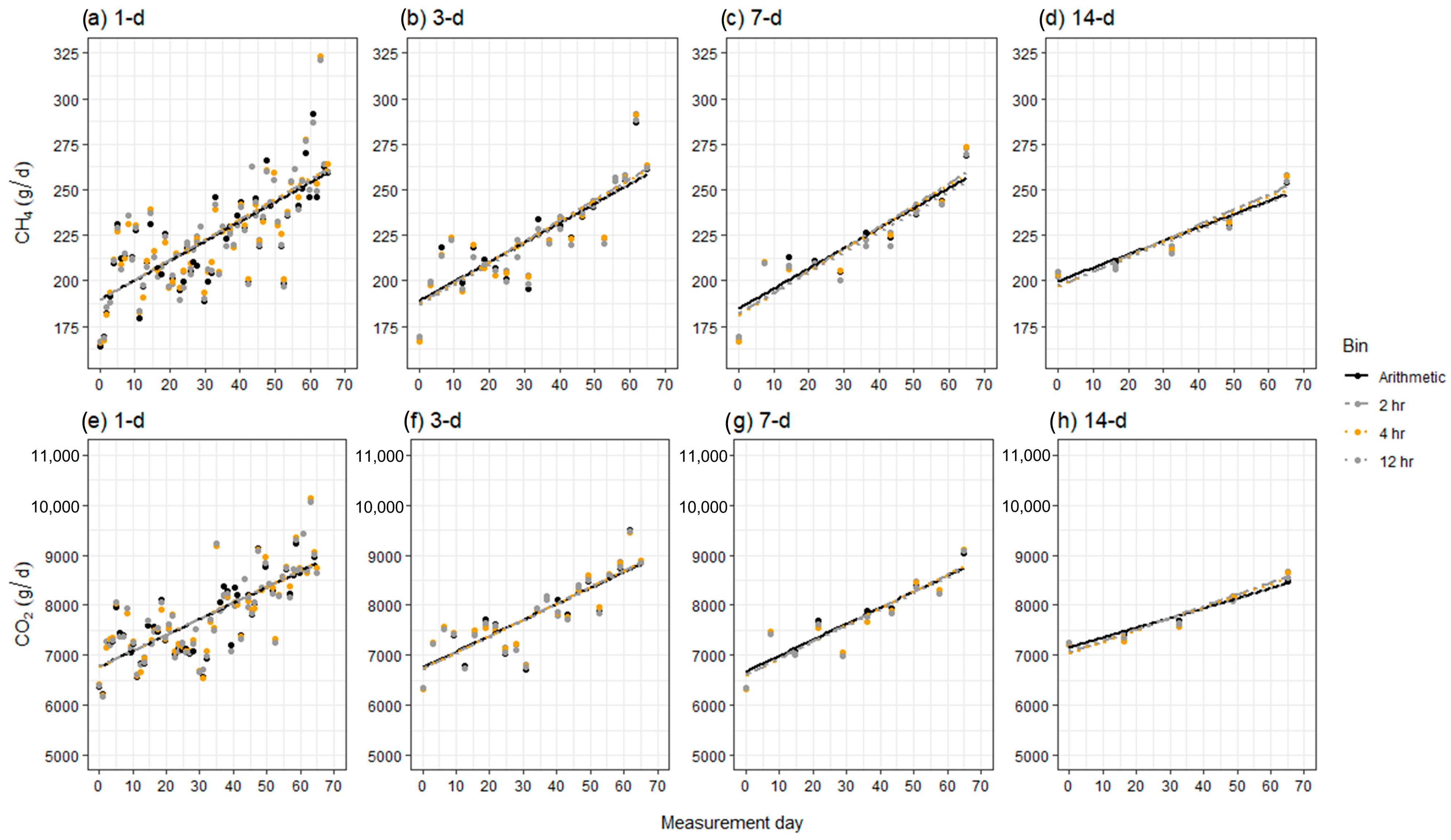
3.1. Data Preprocessing Method Comparison

Enteric emissions measurements spanned ≥55 d during our final pasture-based measurement period with herd access to a single AHCS; therefore, we used these data to compare outcomes to the confinement-based literature. Comparison of gas flux estimates derived from the arithmetic and time-bin averaging methods showed that both preprocessing methods yielded similar values regardless of the time-bin averaging interval for CH4: 2 h (p ≥ 0.64), 4 h (p ≥ 0.46), 12 h (p ≥ 0.66) and CO2: 2 h (p ≥ 0.68), 4 h (p ≥ 0.60), 12 h (p ≥ 0.81; Table 1). Individual animal correlations between arithmetic averaging and time-of-day bin averaging methods were found to be greater than 0.91 across test-length periods (Figure 1), indicating a linear association between the preprocessing estimates under grazing conditions. The arithmetic averaging method was used in subsequent analysis based on these findings.

3.2. Test Period Length Averaging Evaluation

The proportion of animals that visited AHCS in at least five of six possible 4 h time-of-day bins was also calculated for each production setting and AHCS unit exposure period (Table 2). With a 1 d average, only 30% of the animals visited at least five of the six possible 4 h time-of-day bins while acclimating in the feedlot pens. However, with 3, 7, and 14 d test period lengths, averaging 69%, 80%, and 83%, respectively, of the animals visited within at least five of the six time-of-day bins, indicating that animals visited at most times of the day, especially over 7 and 14 d periods. When animals had access to two AHCS units in the initial pasture measurement period, 1 d averaging yielded 4.5% of the animals visited in at least five of the six possible 4 h time-of-day bins, whereas 3, 7, and 14 d averaging returned 21.8%, 24.5%, and 46%, respectively. In the final pasture measurement period with one AHCS per group, 1 d averaging resulted in only 11.8% of the animals visiting AHCS in at least five of the six possible time bins, whereas 3, 7, and 14 d averaging returned 57.3%, 64.5%, and 64.5%, respectively.
While acclimating to AHCS in feedlot pens, the 110 animals produced a total of 2721 visit fluxes by visiting the AHCS during 28 d and averaged 1.99, 4.07, 8.15, and 15.0 visits per animal for 1, 3, 7, and 14 d test period length averaging periods, respectively (Table 2). During the initial pasture measurement period with two AHCS units available to a single group, Group 1 produced 743 visit fluxes by visiting one of two available AHCS over 33 d of measurement, while Group 2 produced 64 visit fluxes over 7 d of measurement. In this period, with access to two AHCS per group, visit fluxes averaged 1.86, 3.90, 6.37, and 8.54 visits per animal for 1, 3, 7, and 14 d averaging periods, respectively. During the final pasture measurement period with one AHCS unit available to a single group of 50 (Group 1) or 60 (Group 2) hd, Group 1 produced 1665 visit fluxes by visiting one AHCS over 55 d of measurement while Group 2 produced 1925 visit fluxes over 59 d. With access to one AHCS per group, 1.65, 3.56, 7.46, and 13.2 visits per animal resulted in 1, 3, 7, and 14 d test period length averaging periods, respectively. Summary statistics for each group are available in Table 2.

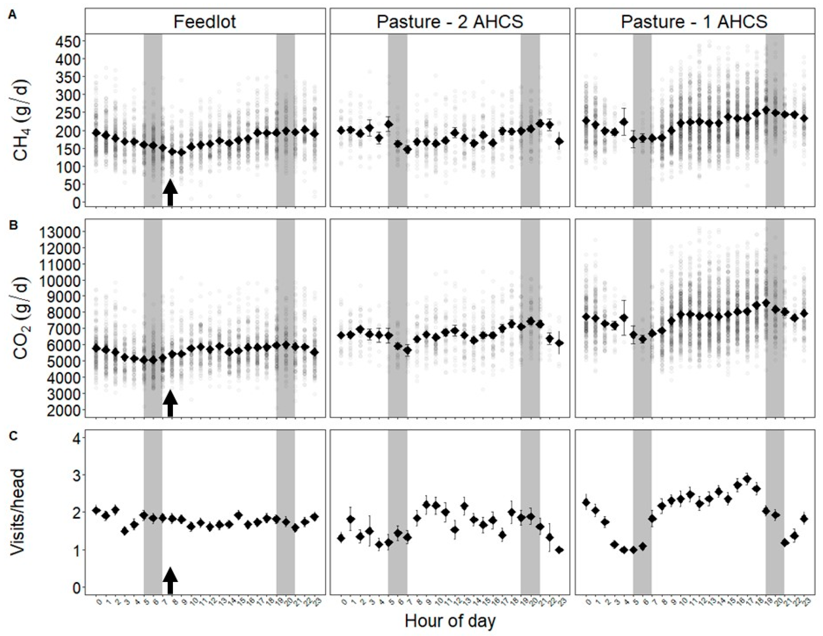
3.3. Gas Flux and AHCS Visitation Variability in Different Production Environments

Despite only having little more than one AHCS unit visit per day, the diurnal pattern in CH4 emissions was likely captured in the confinement production setting because the time of the day that the visit occurred varied from day to day. This pattern can be seen in the density plot presented in Figure 2, where the probability of a visit occurring was spread across all hours of the day. When animals had access to two AHCS units in the initial pasture-based measurement period, the probability of a visit was halved (~0.04 to 0.02) from 2100–0600 relative to confinement, while the probability of a visit increased from ~0.04 to 0.055 and was more evenly spread from 0900 to 2000. A more pronounced bell-curved distribution of visits across the day is evident for the final pasture-based measurement period, when each group had access to a single AHCS simultaneously, indicating that the probability of a visit occurring is greatest from 0900 to 1800 with a probability of more than 0.05. A comparison of density plots for two AHCS vs. one AHCS suggests the probability of a visit to an AHCS on pasture is greater from 0100 to 0800 and from 1800 to 2000 when access to two AHCS units is available.
Figure 3 presents the means and SE for CH4 and CO2 production and visits per animal per hour for each period of this study. Interestingly, there is a wide range of diurnal CH4 patterns when comparing data collected from confined cattle with those from pastured cattle. In confinement, cattle emissions increased post-feeding starting at about 0900 with a maximum CH4 emission estimate over the night to early morning (1700 to 0100) and a minimum CH4 estimate immediately before feeding (0300 to 0900). In contrast, measurements conducted on pasture, irrespective of AHCS availability (i.e., access to one vs. two AHCS), showed a post-sunrise maximum CH4 estimate from 0800 to 1100 and a second peak from 1500 to 2000 with a pre-sunrise minimum CH4 estimate over the late night through early morning (2100–0700). The difference between mean maximum and minimum emissions estimates expressed as a percentage of the minimum estimate provides insight into the diurnal variation in emissions. In pasture measurements, CH4 estimate maximums were 21.3% and 10.1% of the minimum for measurements conducted with animal access to two and one AHCS, respectively, whereas for confinement measurements, CH4 estimate maximums were 41.9% of the minimum. The diurnal patterns of CO2 were less drastic than CH4 (Figure 3); however, cattle in confinement had greater diurnal variation than cattle on pasture. Under grazing conditions, the maximum CO2 was 4.88% greater than the minimum CO2 estimate for confinement measurements. Maximum CO2 emissions were 3.25% and 3.49% greater than the minimum estimates for pasture measurements for animals with access to two and one AHCS, respectively. While cattle grazing had a lower range in gas flux estimates than when they were housed in confinement, they favored using the AHCS at particular times of the day, typically with a peak usage at 0900 to 1200 and another at 1600 to 1800. The pattern of AHCS usage on pasture was less consistent with data collected in confinement, where AHCS visits were lowest from 0300 to 0400, representing the period before feeding, and greatest usage from late night to early morning (2300–0200).

4. Discussion

4.1. Importance of Accounting for Diurnal Variation Across Production Settings

Providing adequate estimates of enteric emissions from multiple visits to AHCS is dependent on two critical factors: (1) the extent of diurnal variation in the production of gas and (2) how closely AHCS visits are distributed across the day. Although researchers attempt to distribute AHCS visits throughout the day by setting a minimum amount of allowable time between each AHCS visit (e.g., 4 h [37]), this step may not be adequate, especially if animals are not visiting the AHCS multiple times a day. The current study aimed to employ AHCS data collected across confinement- and grazing-based production settings to demonstrate the extent of variability of daily enteric emissions and AHCS visitation in these two production settings and to provide insight into how recommendations from confinement-based research carryover to grazing-based enteric emissions measurements.
In a feedlot system, Manafiazar et al. (2017) proposed the time-bin averaging method to counter this AHCS data preprocessing issue, which continues to be implemented in confined settings [37]. In this cross-production setting study, the difference observed between time bin averaged and simple arithmetic averaged estimates shed light on how vital accounting for diurnal variation was for each gas under evaluation and various production settings where livestock was managed. For instance, the estimates of CO2 were small across all production settings investigated in the current study, indicating that accounting for diurnal variation for CO2 was not as important. This result for CO2 estimates across the different production settings was likely driven by low diurnal variation, which ranged from 3.49% to 4.88%. This outcome of low variance is expected as the production of CO2 is a function of metabolism and ruminal fermentation, whereas enteric emission of CH4 is solely a product of ruminal fermentation [38]. On the other hand, the estimates of enteric CH4 production from the two preprocessing methods varied considerably, but less so for grazing measurements than measurements from confinement housing. This outcome was also reported by Manafiazar et al. (2017), who found that simple arithmetic and time-bin averaging estimated CH4 emissions after 14 d of measurements only differed by 4.6 g/d or 2.3% of the arithmetic averaged estimate when using beef heifers fed a 90% barley (Hordeum vulgare) silage diet. This result is particularly interesting because, despite the small difference between the two data pre-processing methods, Manafiazar et al. (2017) maintained their recommendation that time-bin averaging be used over arithmetic averaging. In the current study, arithmetic and time-bin averaging estimated CH4 emissions after 14-d of measurements only differed by 2.7 g/d or 1.2% of the arithmetic averaged estimate for grazing steers on an intensively managed, improved cool-season grass-dominated pasture. The smaller difference between CH4 estimated by arithmetic averaging compared with the time-bin averaging approach for the grazing measurements compared with measurements from confinement is likely due to the lower diurnal variation in grazing-based enteric emissions. This finding may indicate that accounting for diurnal variation through data preprocessing is less critical in grazing than confinement.
In confined settings, researchers have proposed the calculation of the number of 4 h time bins out of six time bins where visits have occurred in a certain time as a means to incorporate diurnal variation when censoring individual animal data prior to conducting statistical analysis [17,18]. For example, Beauchemin, Tamayao, Rosser, Terry, and Gruninger [18] removed animals with missing data for two or more of the six time bins per period of interest before conducting statistical analysis. This data preprocessing approach has not been executed for grazing animals on pastureland. In the current experiment, it took 7 d for two-thirds of the steers housed in confinement to visit AHCS for at least five of six time bins, with one group reaching this threshold for all individuals within 14 d. In contrast, this metric ranged from 8.3% to 44% for all animals across groups after 7 d on pasture in the initial dual AHCS access subperiod. Moreover, the group with 33 d of measurements in this two-AHCS unit subperiod only reached 46% of animals visiting at least five of six time bins with two 14 d averaging periods. Additionally, after 45 d from confinement housing, groups exhibited 60 to 70% of animals meeting this five of six time-bin threshold after 7 d and with no improvement at 14 d for the final grazing measurement subperiod, where animals access a single AHCS unit. We hypothesize that the extent to which diurnal variation of visits and concomitant CH4 emissions is represented on pastureland is governed by herd social cues (i.e., timing of grazing bouts and waterer visits) that are muted in confinement [28]; however, further research is necessary to confirm this supposition.
The diurnal variation of CH4 emissions from AHCS measurements on pasture ranged from 10.1% to 21.3% in the current study. In the grazing measurements, the maximum CH4 estimates occurred from 0800 to 1100 h and a second peak from 1500 to 2000 h, while minimum CH4 estimates occurred over the late night through early morning (2100–0700). In a study using crossbred Bos taurus steers grazing native tallgrass prairie pastures (72.1% NDF; 9.6% CP), Beck et al. [39] determined a maximum CH4 estimate occurred at 2100 to 2400 and a minimum at 1500 to 1800, with a 21% difference between minimum and maximum estimates collected from August to October. This previous work is most like the current study, which measured emissions via an AHCS unit from steers grazing improved perennial cool-season grass-dominated pasture (~70% NDF; ~10% CP [8]) from 8 July through 25 October, with up to a 21.3% difference between the minimum and maximum CH4 estimates. Moreover, emissions measurements by Beck et al. (2019) also exhibited two peak CH4 estimates in the diurnal pattern, with one reported from 2100 through 2400 and another not reported but visually detected from their figures at 1200 to 1400. This outcome suggests that grazing cattle show multiple peak CH4 estimates in their diurnal pattern of enteric emissions, which would be 2–3 h after daily grazing bouts. Grazing cattle are known to exhibit multiple grazing bouts a day during the growing season [40,41], which would lead one to surmise multiple AHCS visits a day are necessary to represent enteric CH4 emissions accurately on grazing-based production systems. Furthermore, the similarity between each study’s pasture nutritive quality may explain the ≤21.3% diurnal variation observed in both studies. This similarity in diurnal variation of steer emissions may not have been observed if the quality of the forage resource was substantially different. For instance, high-fiber, low-digestibility forages can result in lower passage rates and more differentiated grazing bouts than a more digestible forage resource [41,42]. Therefore, we posit that the extent to which diurnal variation of CH4 emissions occurs from grazing cattle is dependent on the nutritive quality of the forage base [43]; however, further research is necessary for confirmation of this prediction.
The rate of enteric CH4 emission is not constant over 24 h in confined production environments, with flux patterns affected by feed allowance and feeding frequency [43,44]. For instance, Jonker, Molano, Antwi, and Waghorn [44] compared feeding 1 to 4 times a day to ad libitum intake on the hourly enteric CH4 emission by beef cattle fed an alfalfa (Medicago sativa) silage in confinement using AHCS technology. They reported that with a single feeding, the CH4 emission rate varied by as much as 6.3-fold. In contrast, the CH4 emission rate only varied by 4.0 fold with ad libitum intake [44]. In our analysis of diurnal variation, the mean maximum CH4 estimate from the initial confinement period of this experiment was 41.9% of the mean minimum CH4 estimate. Furthermore, the maximum CH4 estimates occurred at least 2–3 h after the 0700–0800 feeding window, starting at 0900 and steadily increasing over the remainder of the day until 0100 of the next day. This finding is expected as a distinct nadir in CH4 emissions is widely known to occur prior to feeding, and peak estimates around 3 to 6 h after feeding due to the peak of ruminal fermentation [17,27,45], which is like the current analysis.

4.2. Importance of Accounting for Diurnal Variation Across Experimental Conditions

The current study evaluated AHCS visit frequency, test length averaging efficacy, and diurnal variation of emissions and AHCS visitation in a grazing environment utilizing two experimental conditions: herd access to two AHCS units and herd access to a single AHCS unit. Two AHCS units were initially available to each group to measure emissions equally over two study groups on pasture, but AHCS placement was staggered every two weeks to balance visitation and concomitant emissions measures across groups. Therefore, one group had access to two AHCS units, while enteric emissions for the other group were not measured for two weeks. The idea behind this plan was that animals would have more opportunities to visit AHCS across the day, as individuals would not wait in line as long to visit AHCS as compared to the herd with access to a single AHCS unit. Figure 2 shows that this prediction was met with visit probability being evenly spread over the day when a group had access to two AHCS. However, this approach of staggering AHCS availability across two groups negatively impacted overall data collection in this phase of the current experiment. One group had access to two AHCS units for 33 d, while the second group accessed two AHCS units for only 7 d due to AHCS mechanical problems. The discrepancy between the two groups’ total days of data collection only allowed for group comparison of visitation frequency and the percentage of individual steers with five of six time bins measured for the 7 d test length averaging period. This discrepancy resulted in an 85% increase in visitation frequency as Group 1’s 7 d averaging estimate resulted from four 7 d averaging periods, while the 7 d average from Group 2 was not replicated. Furthermore, the lack of replication in 7 d averaging periods resulted in an 81% decrease in the number of animals with five of six time bins measured when compared to Group 1 with replicated 7 d averaging periods. This outcome demonstrates that the successful staggering of AHCS availability to individual groups to balance sample size across groups is fully dependent on AHCS unit reliability.
As researchers realized that the dual AHCS unit arrangement and the staggering approach were not beneficial toward adequately measuring emissions for each group, a switch to each group having access to a single AHCS unit was made for the remainder of this experiment. This change in experimental condition provided each group with at least 55 d of gas flux measurements. In this final phase of grazing measurements, a total of three 14 d test length averaging periods were represented for each group. This opportunity allowed for the comparison of standard deviations across test length averaging periods, e.g., from 1 to 14 d test period lengths shown in Table 1 with outcomes in Manafiazar, Zimmerman, and Basarab [17] and Harrison [46]. As the test length averaging period increased from 1 to 14 d, the standard deviation of emissions decreased by 42% and 32% for CH4 and CO2, respectively. However, the SD value decreased slightly more between 1 and 3 d (CH4:18%, CO2:15%) than between 7 and 14 d (CH4: 15%, CO2: 12%) averaging periods. When the difference in standard deviations of CH4 emissions from 1 to 3 d and 7 to 14 d test length averages (i.e., 19%) are compared to the fed beef heifers reported by Manafiazar et al. (2017), e.g., 88% for CH4, lower and consistent variability across test length comparisons on pasture are apparent. This finding suggests that the data preprocessing approach of test period length averaging is not as important in a grazing context as it is for a confined setting with a high-forage diet, as lower variation in grazing measurements is present to account for when aggregating visit fluxes over a given time period.

5. Conclusions

The results of this experiment suggest that the time-bin averaging approach to data preprocessing when compared to simple arithmetic averaging in intensively managed pasture-based AHCS experiment, was not necessarily due to less diurnal variation in enteric emissions for grazing steers on pasture. In addition, although visitation probability increased with a herd having access to two AHCS compared to one AHCS unit, findings suggest that the staggering of AHCS unit availability to individual groups to balance sample size across groups is fully dependent on AHCS unit reliability. Therefore, it is recommended to employ a single AHCS unit per group to ensure adequate data collection when AHCS availability is scarce. This recommendation is intended to save researchers time inefficiently deploying AHCS units to measure pasture-based enteric gas flux in response to GHG reduction practices. Due to the lack of diurnal variation in pasture-based emissions measurements in the current study, 7 d test period length averaging appears adequate for representative gas flux estimates for steers on pasture. In other words, when accounting for time-dependent effects in a 70 d study, one should feel confident breaking the dataset down to 7 d test length intervals. It is hoped that the findings herein will standardize AHCS data preprocessing, thereby maintaining consistency across experiments and research groups.

Author Contributions

Conceptualization, E.J.R., P.H.V.C., S.E.P. and K.R.S.-L.; methodology, E.J.R., P.H.V.C., E.C.M., W.A.S., A.M.S., S.E.P. and K.R.S.-L.; formal analysis, E.J.R., J.d.J.V. and S.E.P.; investigation, P.H.V.C., E.C.M., W.A.S., A.M.S., S.E.P., E.J.R., A.J. and K.R.S.-L.; data curation, A.M.S., E.C.M., W.A.S., A.J. and E.J.R.; writing—original draft preparation, E.J.R., P.H.V.C., S.E.P., J.d.J.V. and K.R.S.-L.; writing—review and editing, E.J.R., P.H.V.C., S.E.P., J.d.J.V. and K.R.S.-L.; supervision, P.H.V.C., E.J.R. and K.R.S.-L.; project administration, P.H.V.C., E.C.M., W.A.S., A.M.S., S.E.P., E.J.R. and K.R.S.-L.; funding acquisition, E.J.R., P.H.V.C., S.E.P. and K.R.S.-L. All authors have read and agreed to the published version of the manuscript.

Funding

This research was funded by Elanco Animal Health: ELA230898.

Institutional Review Board Statement

This study was conducted in accordance with the Declaration of Helsinki and approved by the Institutional Animal Care and Use Committee of Colorado State University (protocol code 4456, approved on 22 May 2023). The acclimation period was conducted at the Climate Smart Research Facility (CSRF), and the measurement period was conducted at center pivot-irrigated pasture located at the Colorado State University Agricultural Research Development and Education Center (ARDEC).

Informed Consent Statement

Not applicable.

Data Availability Statement

The data presented in this study are available upon request from the corresponding author.

Acknowledgments

This research was made possible by Colorado State University AgNext and Agricultural Experimental Station.

Conflicts of Interest

The authors declare no real or perceived conflicts of interest.

References

  1. Pelton, R.E.O.; Kazanski, C.E.; Keerthi, S.; Racette, K.A.; Gennet, S.; Springer, N.; Yacobson, E.; Wironen, M.; Ray, D.; Johnson, K.; et al. Greenhouse gas emissions in US beef production can be reduced by up to 30% with the adoption of selected mitigation measures. Nat. Food 2024, 5, 787–797. [Google Scholar] [CrossRef]
  2. Hammond, K.J.; Crompton, L.A.; Bannink, A.; Dijkstra, J.; Yáñez-Ruiz, D.R.; O’Kiely, P.; Kebreab, E.; Eugène, M.A.; Yu, Z.; Shingfield, K.J.; et al. Review of current in vivo measurement techniques for quantifying enteric methane emission from ruminants. Anim. Feed Sci. Technol. 2016, 219, 13–30. [Google Scholar] [CrossRef]
  3. Rotz, C.A.; Asem-Hiablie, S.; Place, S.; Thoma, G. Environmental footprints of beef cattle production in the United States. Agric. Syst. 2019, 169, 1–13. [Google Scholar] [CrossRef]
  4. Raynor, E.J.; Kutz, M.; Thompson, L.R.; Carvalho, P.H.V.; Place, S.E.; Stackhouse-Lawson, K.R. Impact of growth implants and low-level tannin supplementation on enteric emissions and nitrogen excretion in grazing steers. Transl. Anim. Sci. 2024, 8, txae115. [Google Scholar] [CrossRef]
  5. Schilling-Hazlett, A.; Raynor, E.J.; Thompson, L.; Velez, J.; Place, S.; Stackhouse-Lawson, K. On-Farm Methane Mitigation and Animal Health Assessment of a Commercially Available Tannin Supplement in Organic Dairy Heifers. Animals 2024, 14, 9. [Google Scholar] [CrossRef]
  6. Dressler, E.A.; Bormann, J.M.; Weaber, R.L.; Rolf, M.M. Use of methane production data for genetic prediction in beef cattle: A review. Transl. Anim. Sci. 2024, 8, txae014. [Google Scholar] [CrossRef] [PubMed]
  7. Vargas, J.d.J.; Swenson, M.; Place, S.E. Determination of gas flux and animal performance test duration of growing cattle in confined conditions. Transl. Anim. Sci. 2024, 8, txae056. [Google Scholar] [CrossRef] [PubMed]
  8. Vargas, J.d.J.; Carvalho, P.H.V.; Raynor, E.J.; Martins, E.C.; Souza, W.A.; Shadbolt, A.M.; Stackhouse-Lawson, K.R.; Place, S.E. Determination of gas flux of growing steers under intensive grazing conditions. Transl. Anim. Sci. 2024, 8, txae119. [Google Scholar] [CrossRef] [PubMed]
  9. Vargas, J.; Menezes, T.; Auvermann, B.; Derner, J.; Thoma, G.; Hales, K.; Johnson, K.; Leytem, A.; Place, S.; Plaut, J.; et al. Net zero initiative in U.S. beef and dairy systems: Integrative on-farm recommendations for greenhouse gas reduction. Environ. Res. Commun. 2024, 6, 101010. [Google Scholar] [CrossRef]
  10. Hristov, A.N.; Kebreab, E.; Niu, M.; Oh, J.; Bannink, A.; Bayat, A.R.; Boland, T.M.; Brito, A.F.; Casper, D.P.; Crompton, L.A. Symposium review: Uncertainties in enteric methane inventories, measurement techniques, and prediction models. J. Dairy Sci. 2018, 101, 6655–6674. [Google Scholar] [CrossRef] [PubMed]
  11. Thompson, L.R.; Rowntree, J.E. Methane sources, quantification, and mitigation in grazing beef systems. Appl. Anim. Sci. 2020, 36, 556–573. [Google Scholar] [CrossRef]
  12. Della Rosa, M.; Jonker, A.; Waghorn, G. A review of technical variations and protocols used to measure methane emissions from ruminants using respiration chambers, SF6 tracer technique and GreenFeed, to facilitate global integration of published data. Anim. Feed Sci. Technol. 2021, 279, 115018. [Google Scholar] [CrossRef]
  13. Waghorn, G.C.; Jonker, A.; Macdonald, K.A. Measuring methane from grazing dairy cows using GreenFeed. Anim. Prod. Sci. 2016, 56, 252–257. [Google Scholar] [CrossRef]
  14. Thompson, L.R.; Maciel, I.C.F.; Rodrigues, P.D.R.; Cassida, K.A.; Rowntree, J.E. Impact of forage diversity on forage productivity, nutritive value, beef cattle performance, and enteric methane emissions. J. Anim. Sci. 2021, 99, skab326. [Google Scholar] [CrossRef] [PubMed]
  15. Raynor, E.J.; Schilling-Hazlett, A.; Place, S.E.; Martinez, J.V.; Thompson, L.R.; Johnston, M.K.; Jorns, T.R.; Beck, M.R.; Kuehn, L.A.; Derner, J.D.; et al. Snapshot of Enteric Methane Emissions from Stocker Cattle Grazing Extensive Semiarid Rangelands. Rangel. Ecol. Manag. 2024, 93, 77–80. [Google Scholar] [CrossRef]
  16. Beck, M.R.; Thompson, L.R.; Proctor, J.A.; Reuter, R.R.; Gunter, S.A. Recommendations on visit duration and sample number requirements for an automated head chamber system. J. Anim. Sci. 2024, 102, skae158. [Google Scholar] [CrossRef] [PubMed]
  17. Manafiazar, G.; Zimmerman, S.; Basarab, J.A. Repeatability and variability of short-term spot measurement of methane and carbon dioxide emissions from beef cattle using GreenFeed emissions monitoring system. Can. J. Anim. Sci. 2017, 97, 118–126. [Google Scholar] [CrossRef]
  18. Beauchemin, K.A.; Tamayao, P.; Rosser, C.; Terry, S.A.; Gruninger, R. Understanding variability and repeatability of enteric methane production in feedlot cattle. Front. Anim. Sci. 2022, 3, 1029094. [Google Scholar] [CrossRef]
  19. Gunter, S.A.; Beck, M.R. Measuring the respiratory gas exchange by grazing cattle using an automated, open-circuit gas quantification system. Transl. Anim. Sci. 2018, 2, 11–18. [Google Scholar] [CrossRef] [PubMed]
  20. Dressler, E.A.; Bormann, J.M.; Weaber, R.L.; Rolf, M.M. Characterization of the number of spot samples required for quantification of gas fluxes and metabolic heat production from grazing beef cows using a GreenFeed. J. Anim. Sci. 2023, 101, skad176. [Google Scholar] [CrossRef] [PubMed]
  21. U.S. Department of Agriculture. Summary Report: 2007 National Resources Inventory; Natural Resources Conservation Service: Washington, DC, USA; Center for Survey Statistics and Methodology, Iowa State University: Ames, IA, USA, 2009. [Google Scholar]
  22. Cullison, A. Effect of physical form of the ration on steer performance and certain rumen phenomena. J. Anim. Sci. 1961, 20, 478–483. [Google Scholar] [CrossRef]
  23. Gerrish, J. Management-Intensive Grazing: The Grassroots of Grass Farming; Green Park Press: Hyde Park, VT, USA, 2004. [Google Scholar]
  24. Jonker, A.; Waghorn, G. Guidelines for Estimating Methane Emissions from Individual Ruminants Using: GreenFeed, ’sniffers’, Hand-Held Laser Detector and Portable Accumulation Chambers; Ministry for Primary Industries = Manatū Ahu Matua: Wellington, New Zealand, 2020. [Google Scholar]
  25. Velazco, J.; Mayer, D.; Zimmerman, S.; Hegarty, R. Use of short-term breath measures to estimate daily methane production by cattle. Animal 2016, 10, 25–33. [Google Scholar] [CrossRef]
  26. Hegarty, R.S. Applicability of short-term emission measurements for on-farm quantification of enteric methane. Animal 2013, 7 (Suppl. S2), 401–408. [Google Scholar] [CrossRef] [PubMed]
  27. Hales, K.E.; Cole, N.A. Hourly methane production in finishing steers fed at different levels of dry matter intake. J. Anim. Sci. 2017, 95, 2089–2096. [Google Scholar] [CrossRef] [PubMed]
  28. Gunter, S.; Bradford, J. Influence of sampling time on carbon dioxide and methane emissions by grazing cattle. Proc. West. Sect. Am. Soc. Anim. Sci. 2015, 66, 201–203. [Google Scholar]
  29. Hammond, K.; Humphries, D.; Crompton, L.; Kirton, P.; Green, C.; Reynolds, C. Methane emissions from growing dairy heifers estimated using an automated head chamber (GreenFeed) compared to respiration chambers or SF6 techniques. Adv. Anim. Biosci. 2013, 4, 391. [Google Scholar]
  30. Vargas, J.; Ungerfeld, E.; Muñoz, C.; DiLorenzo, N. Feeding Strategies to Mitigate Enteric Methane Emission from Ruminants in Grassland Systems. Animals 2022, 12, 1132. [Google Scholar] [CrossRef] [PubMed]
  31. Brennan, J.R.; Parsons, I.L.; Harrison, M.; Menendez, H.M., III. Development of an application programming interface to automate downloading and processing of precision livestock data. Transl. Anim. Sci. 2024, 8, txae092. [Google Scholar] [CrossRef]
  32. Shawver, C.J.; Ippolito, J.A.; Brummer, J.E.; Ahola, J.K.; Rhoades, R.D. Soil health changes following transition from an annual cropping to perennial management-intensive grazing agroecosystem. Agrosystems Geosci. Environ. 2021, 4, e20181. [Google Scholar] [CrossRef]
  33. Huhtanen, P.; Cabezas-Garcia, E.H.; Utsumi, S.; Zimmerman, S. Comparison of methods to determine methane emissions from dairy cows in farm conditions. J. Dairy Sci. 2015, 98, 3394–3409. [Google Scholar] [CrossRef] [PubMed]
  34. Arthur, P.F.; Barchia, I.M.; Weber, C.; Bird-Gardiner, T.; Donoghue, K.A.; Herd, R.M.; Hegarty, R.S. Optimizing test procedures for estimating daily methane and carbon dioxide emissions in cattle using short-term breath measures. J. Anim. Sci. 2017, 95, 645–656. [Google Scholar] [CrossRef]
  35. R Development Core Team. R: A Language and Environment for Statistical Computing; R Foundation for Statistical Computing: Vienna, Austria, 2023. [Google Scholar]
  36. Wickham, H. ggplot2. Wiley Interdiscip. Rev.-Comput. Stat. 2011, 3, 180–185. [Google Scholar] [CrossRef]
  37. Alemu, A.W.; Schreck, A.L.; Booker, C.W.; MCGinn, S.M.; Pekrul, L.K.D.; Kindermann, M.; Beauchemin, K.A. Use of 3-nitrooxypropanol in a commercial feedlot to decrease enteric methane emissions from cattle fed a corn-based finishing diet. J. Anim. Sci. 2021, 99, skaa394. [Google Scholar] [CrossRef] [PubMed]
  38. Van Soest, P.J. Nutritional Ecology of the Ruminant; Cornell University Press: Ithaca, NY, USA, 1994. [Google Scholar]
  39. Beck, M.R.; Thompson, L.R.; Williams, G.D.; Place, S.E.; Gunter, S.A.; Reuter, R.R. Fat supplements differing in physical form improve performance but divergently influence methane emissions of grazing beef cattle. Anim. Feed. Sci. Technol. 2019, 254, 114210. [Google Scholar] [CrossRef]
  40. Raynor, E.J.; Derner, J.D.; Soder, K.J.; Augustine, D.J. Noseband sensor validation and behavioural indicators for assessing beef cattle grazing on extensive pastures. Appl. Anim. Behav. Sci. 2021, 242, 105402. [Google Scholar] [CrossRef]
  41. Gregorini, P. Diurnal grazing pattern: Its physiological basis and strategic management. Anim. Prod. Sci. 2012, 52, 416–430. [Google Scholar] [CrossRef]
  42. Archimède, H.; Eugène, M.; Magdeleine, C.M.; Boval, M.; Martin, C.; Morgavi, D.; Lecomte, P.; Doreau, M. Comparison of methane production between C3 and C4 grasses and legumes. Anim. Feed Sci. Technol. 2011, 166, 59–64. [Google Scholar] [CrossRef]
  43. Hammond, K.J.; Waghorn, G.C.; Hegarty, R.S. The GreenFeed system for measurement of enteric methane emission from cattle. Anim. Prod. Sci. 2016, 56, 181–189. [Google Scholar] [CrossRef]
  44. Jonker, A.; Molano, G.; Antwi, C.; Waghorn, G. Feeding lucerne silage to beef cattle at three allowances and four feeding frequencies affects circadian patterns of methane emissions, but not emissions per unit of intake. Anim. Prod. Sci. 2014, 54, 1350–1353. [Google Scholar] [CrossRef]
  45. Beck, M.R.; Proctor, J.A.; Kasuske, Z.; Smith, J.K.; Gouvêa, V.N.; Lockard, C.L.; Min, B.; Brauer, D. Effects of replacing steam-flaked corn with increasing levels of malted barley in a finishing ration on feed intake, growth performance, and enteric methane emissions of beef steers. Appl. Anim. Sci. 2023, 39, 525–534. [Google Scholar] [CrossRef]
  46. Harrison, M. GreenFeed Manual; C-Lock, Inc.: Rapid City, SD, USA, 2024; pp. 46–49. [Google Scholar]
Figure 1. Test period length relationships between gas production and measurement day for arithmetic averaging and time-bin averaging preprocessing methods during grazing measurements of yearling steers accessing a single automated head-chamber system (AHCS) for CH4 (ad) and CO2 (eh) gas flux measurements.
Grasses 04 00012 g001
Figure 2. Density plot illustrating the probability of an automated head chamber system (AHCS) visit for 110 yearling steers acclimating in confinement (dashed) and utilizing a portable AHCS on pasture with exposure to two AHCS units (purple) and one AHCS unit (green) during the 2023 grazing season at Colorado State University Agricultural Research and Development Education Center in Fort Collins, Colorado, United States.
Grasses 04 00012 g002
Figure 3. The mean and standard error of the mean (SE) for yearling steer CH4 emissions (A), CO2 emissions (B), and automated head chamber system (AHCS) visits (C) based on arithmetic averaging for each measurement period and averaged across both groups. Arrows indicate feeding time; shaded bars indicate sunrise and sunset, and open points represent raw data for each hour of the day at Colorado State University Agricultural Research and Development Education Center in Fort Collins, Colorado, United States.
Grasses 04 00012 g003
Table 1. Herd averaged fluxes (±SD) from 110 steers using a single automated head chamber system (AHCS) unit on pasture for methane (CH4) and carbon dioxide (CO2) in four test length averaging periods using the arithmetic and time-bin averaging methods.
Bin (Hr) *Averaging Period (d) ^Arithmetic AveragingTime-Bin Averagingr (Anova p)
CH4 (g d−1)CO2 (g d−1)CH4 (g d−1)CO2 (g d−1)CH4 (g d−1)CO2 (g d−1)
21222.76 ± 57.067763.73 ± 1362.18221.39 ± 62.517716.33 ± 1471.960.98 (0.64)0.99 (0.68)
3221.72 ± 46.867737.50 ± 1163.88221.27 ± 60.967726.07 ± 1437.700.98 (0.78)0.99 (0.84)
7220.40 ± 38.717692.08 ± 1039.65221.15 ± 58.427705.87 ± 1383.140.97 (0.99)0.99 (0.99)
14223.22 ± 33.097754.92 ± 919.03221.99 ± 54.737728.54 ± 1283.930.96 (0.61)0.98 (0.73)
41222.76 ± 57.067763.73 ± 1362.18221.51 ± 62.48 7721.83 ± 1470.950.98 (0.67)0.99 (0.72)
3221.72 ± 46.867737.50 ± 1163.88220.76 ± 58.767715.28 ± 1385.100.96 (0.69)0.98 (0.78)
7220.40 ± 38.717692.08 ± 1039.65219.68 ± 54.327676.69 ± 1298.190.94 (0.72) 0.99 (0.85)
14223.22 ± 33.097754.92 ± 919.03221.09 ± 49.917704.21 ± 1197.230.91 (0.46)0.97 (0.60)
121222.76 ± 57.067763.73 ± 1362.18221.82 ± 61.027751.15 ± 1362.180.99 (0.74)0.99 (0.85)
3221.72 ± 46.867737.50 ± 1163.88220.89 ± 54.197744.12 ± 1163.880.97 (0.75)0.99 (0.90)
7220.40 ± 38.717692.08 ± 1039.65218.72 ± 47.497691.01 ± 1039.650.98 (0.66)0.99 (0.84)
14223.22 ± 33.097754.92 ± 919.03221.89 ± 40.867752.42 ± 919.030.97 (0.68)0.99 (0.81)
* Time-bin averaging first averages daily visit data into 4-h time bins (e.g., six bins per day) within each animal and then averages across the time bins within each animal. ^ Averaging period is averaging 1 d total emissions (i.e., CH4 or CO2) across 1, 3, 7, and 14 d periods for each animal.
Table 2. Test period length averaging period visits (mean ± SD, range) for steers that used an automated head chamber system (AHCS) unit and the number and percentage (%) of individual steers that visited automated head chamber system (AHCS) for at least 5 of the 6 possible 4 h time-of-day bins per group for each measurement period. AHCS visits spanned at least 3 min in duration.
GroupMetricMeasurement Period Test Period Length Interval
Location# AHCS Dates; days1-d3-d7-d14-d
1 (n = 50 hd)Visits (n/d)ConfinedOne6/13–7/5/2023; 231.83 ± 1.16; 1–63.51 ± 1.57; 3–166.59 ± 3.29; 4–3112.25 ± 6.58; 5–45
1PastureTwo7/8–8/21/2023; 331.85 ± 0.92; 1–63.20 ± 1.35; 1–134.93 ± 2.67; 1–186.75 ± 4.03; 1–25
1PastureOne8/23–10/16/2023; 551.61 ± 0.82; 1–63.19 ± 1.00; 1–136.79 ± 2.66; 1–2512.62 ± 5.89; 1–43
1%ind. with 5 of 6 time bins measuredConfinedOne6/13–7/05/2023; 2317 (34)37 (74)48 (96)50 (100)
1PastureTwo7/8–8/21/2023; 334 (8)21 (42)22 (44)23 (46)
1PastureOne8/23–10/16/23; 555 (10)31 (62)35 (70)35 (70)
2 (n = 60 hd)Visits (n/d)ConfinedOne6/13–7/10/23; 282.15 ± 1.24; 1–64.36 ± 1.86; 1–179.78 ± 4.95; 1–3117.83 ± 9.83; 1–47
2PastureTwo7/31–8/6/23; 72.06 ± 1.15; 1–53.33 ± 2.04; 1–109.14 ± 7.06; 1–19-
2PastureOne8/24–10/25/23; 591.69 ± 0.85; 1–63.56 ± 1.10; 2–137.16 ± 2.75; 2–2011.76 ± 5.32; 2–34
2%ind. with 5 of 6 time bins measuredConfinedOne6/13–7/10/23; 2816 (26.7)39 (65.0)40 (66.7)40 (66.7)
2PastureTwo7/31–8/6/23; 71 (1.6)3 (5.0)5 (8.3)-
2PastureOne8/24–10/25/23; 598 (13.3)32 (53.3)36 (60.0)36 (60.0)
# indicates the number of automated head chamber system (AHCS) units simultaneously available to group.
Disclaimer/Publisher’s Note: The statements, opinions and data contained in all publications are solely those of the individual author(s) and contributor(s) and not of MDPI and/or the editor(s). MDPI and/or the editor(s) disclaim responsibility for any injury to people or property resulting from any ideas, methods, instructions or products referred to in the content.

