Electricity as a Commodity: Liberalisation Outcomes, Market Concentration and Switching Dynamics

Abstract

We study Portugal’s household electricity retail market after legal liberalisation, quantifying market concentration (Herfindahl–Hirschman Index (HHI) and the four-firm concentration ratio (CR4)), consumer switching, and asymmetric wholesale-to-retail price pass-through. Using monthly data for January 2014–December 2019 (primary sample) and robustness checks for 2008–2022, we compute concentration indices from ERSE supplier shares, analyse switching dynamics, and estimate nonlinear autoregressive distributed lag (NARDL) models that decompose wholesale price changes into positive and negative components. The retail market remains highly concentrated during the primary window (HHI ≈ 6300–6800 using shares expressed as percentages on a 10,000 scale); switching rose after deregulation but stabilised at moderate monthly rates; and long-run pass-through is estimated at β⁺ ≈ 0.55–0.61 for wholesale increases and β⁻ ≈ 0.49 for decreases (Wald tests reject symmetry at conventional levels). Results are robust to alternative concentration metrics, exclusion of 2022, and varied lag orders. Policy implications emphasise tariff simplification, active consumer-activation measures, and regular monitoring of concentration and pass-through metrics.

1. Introduction

Electricity occupies a dual role as both a vital public service and a tradable commodity. Its reliable provision underpins economic and social activity, while its price dynamics influence household welfare, firm competitiveness, and broader macroeconomic stability. Over the past three decades, many European countries have liberalised their electricity sectors, replacing vertically integrated monopolies with wholesale markets and competitive retail supply. The European Union has been a driving force in this process through successive liberalisation packages aimed at unbundling, cross-border integration, and consumer choice [1,2].

Portugal implemented liberalisation gradually, culminating in the full deregulation of the low-voltage segment in 2013. The intended outcomes were to reduce concentration, promote supplier switching, and ensure efficient pass-through of wholesale costs into retail tariffs. Yet international experience demonstrates that these objectives are not always realised. Even in formally liberalised settings, markets may remain concentrated, incumbent suppliers often preserve market power, and wholesale-to-retail price transmission is frequently incomplete or asymmetric [3,4].

Evidence from other EU markets illustrates the diversity of outcomes. The UK experienced significant supplier entry and initially high switching rates, but market consolidation later raised concerns about a “Big Six” oligopoly [5]. Spain liberalised alongside Portugal within the Iberian MIBEL framework, but greater interconnection capacity has sustained higher switching activity and a more competitive retail segment [6]. Ireland’s residential gas and electricity markets remain concentrated, yet targeted consumer activation policies by the Commission for Regulation of Utilities (CRU) have achieved higher switching rates than in Portugal [7]. These comparisons highlight that structural conditions such as interconnection, regulatory design, and consumer engagement strongly influence liberalisation outcomes in small and semi-isolated systems.

The Portuguese case provides a distinctive setting for evaluating these dynamics. The household retail market is dominated by a few suppliers, switching has stabilised at modest levels, and pass-through of wholesale prices may be asymmetric. Understanding these patterns is essential for assessing whether liberalisation has delivered its promised benefits in terms of efficiency, consumer empowerment, and price responsiveness.

This paper addresses three interrelated research questions:

• Market concentration—How have indicators such as the Herfindahl–Hirschman Index (HHI) and the four-firm concentration ratio (CR4) evolved since liberalisation?
• Consumer switching—To what extent have households changed suppliers, and what dynamics characterise these switching patterns?
• Price pass-through—How symmetrically and completely are wholesale price movements reflected in retail tariffs?

Using monthly data from the Energy Services Regulatory Authority (ERSE) [8,9,10,11], the Directorate-General for Energy and Geology (DGEG) [12], and Eurostat, we examine the period 2014–2019, with extended robustness checks covering 2008–2022. We compute concentration indices, analyse supplier switching rates, and estimate an asymmetric autoregressive distributed lag (ARDL) model to measure pass-through. By combining structural market indicators with dynamic econometric modelling, the paper contributes to the literature on electricity market performance in small, liberalised economies and offers evidence to inform regulatory and consumer-protection policies.

Liberalisation of electricity markets has been extensively studied in larger European economies, with evidence pointing to mixed outcomes. References [3,13] note that while liberalisation often increases efficiency, it does not always yield lower consumer prices. The authors of [4] emphasise the persistence of market power in retail markets, while [14] highlights the role of consumer engagement in determining competitive outcomes. Reference [15] examines consumer responsiveness in the electricity sector using a decision support system to evaluate policy scenarios. Results indicate that price signals significantly shape demand, while incentives promoting energy efficiency deliver superior technical, economic, and environmental outcomes compared to reducing retail electricity prices. However, small, semi-isolated systems such as Portugal’s remain underexplored, despite their unique characteristics of high renewable penetration, limited interconnection, and concentrated supplier structures. This study addresses that gap by providing a detailed empirical assessment of Portugal’s household retail electricity market, thereby offering insights that can inform regulatory policy not only domestically but also in other small or structurally similar markets. To that end, this study adopts an integrated analytical framework that synthesises these three perspectives. The economic competition lens guides the selection of structural indicators (HHI, market shares, switching rates, and price trends). The behavioural economics lens informs the interpretation of switching patterns and consumer engagement dynamics. The social–institutional lens situates the findings within broader debates on fairness, inclusion, and regulatory responsiveness. By combining these perspectives, the analysis recognises that liberalisation is not a singular event but a continuous, co-evolutionary process shaped by infrastructure, regulation, and consumer agency. This approach enables a more holistic evaluation of whether the Portuguese retail electricity market has delivered the promised benefits of liberalisation—not only in terms of efficiency and price, but also in relation to participation, equity, and institutional effectiveness.

By integrating structural indicators, behavioural measures, and econometric analysis, this study contributes to the literature on electricity market performance in small liberalised economies. Beyond Portugal, the findings provide lessons for regulators in comparable systems where liberalisation is legally complete but effective competition remains constrained.

2. Materials and Methods

2.1. The Portuguese Electricity System

Portugal’s electricity system operates within the Iberian energy framework, integrating domestic generation, cross-border exchanges, and wholesale trading through the Mercado Ibérico de Electricidade (MIBEL). It is characterised by a high share of renewable generation, a small number of dominant market participants, and a regulated transmission network that interfaces with a liberalised retail segment [6,11].

From a commodity-market perspective, electricity in Portugal shares the fundamental properties of the wider European power sector: non-storability at scale (except via limited pumped-hydro and battery storage), inelastic short-term demand, and the requirement for instantaneous balance between supply and consumption [3,16]. These attributes make wholesale price volatility and system flexibility critical for market functioning and retail price formation.

Generation is dominated by hydroelectric, wind, and solar photovoltaic resources, complemented by natural gas-fired plants that provide dispatchable capacity [11]. Hydroelectric output is highly dependent on annual hydrological conditions, while wind production is seasonally variable but forecastable at short horizons. Solar generation is concentrated in daylight hours with seasonal variation, and combined-cycle gas turbines (CCGT) are used to cover demand peaks and provide balancing services [17].

The national transmission grid is operated by Rede Eléctrica Nacional (REN) under a regulated monopoly model. REN ensures physical balancing, manages interconnections, and coordinates with the Spanish transmission system operator, Red Eléctrica de España, for cross-border operations [18]. Portugal’s interconnection capacity with Spain is significant relative to domestic demand, enabling active participation in MIBEL’s day-ahead and intraday markets. However, interconnection with the broader European network remains limited, making the Iberian Peninsula effectively a semi-isolated zone, which can amplify price effects of local supply–demand imbalances [19].

Wholesale prices are set primarily in MIBEL’s day-ahead market, operated by OMIE using a marginal pricing mechanism. Generators submit supply offers and consumers or their retailers submit demand bids; the market-clearing price is determined by the marginal unit required to meet demand [6]. Intraday markets and balancing services allow adjustments for deviations between forecasted and actual system conditions.

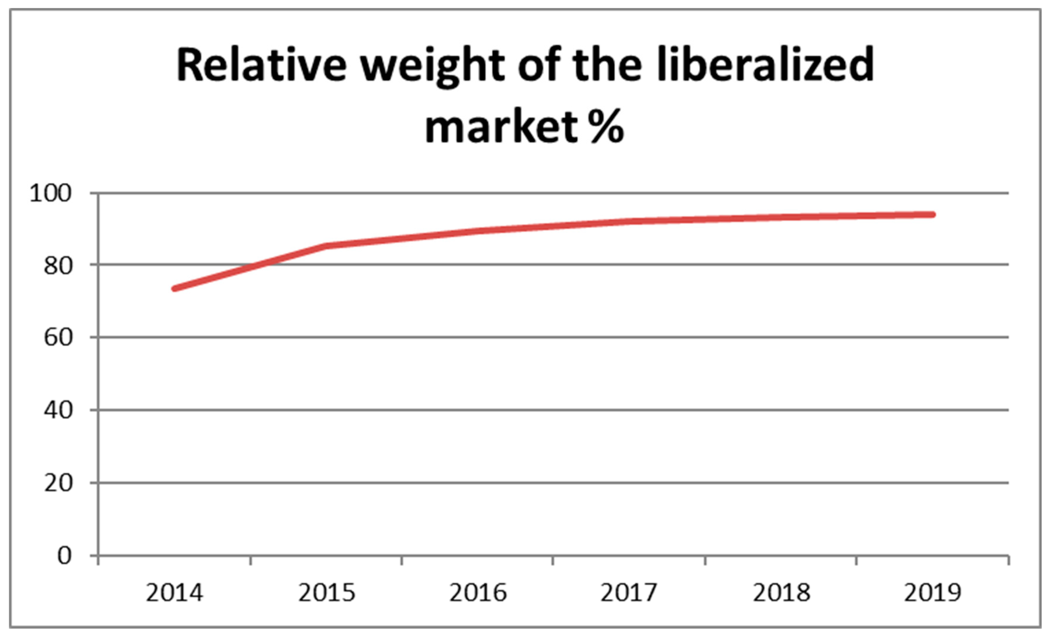
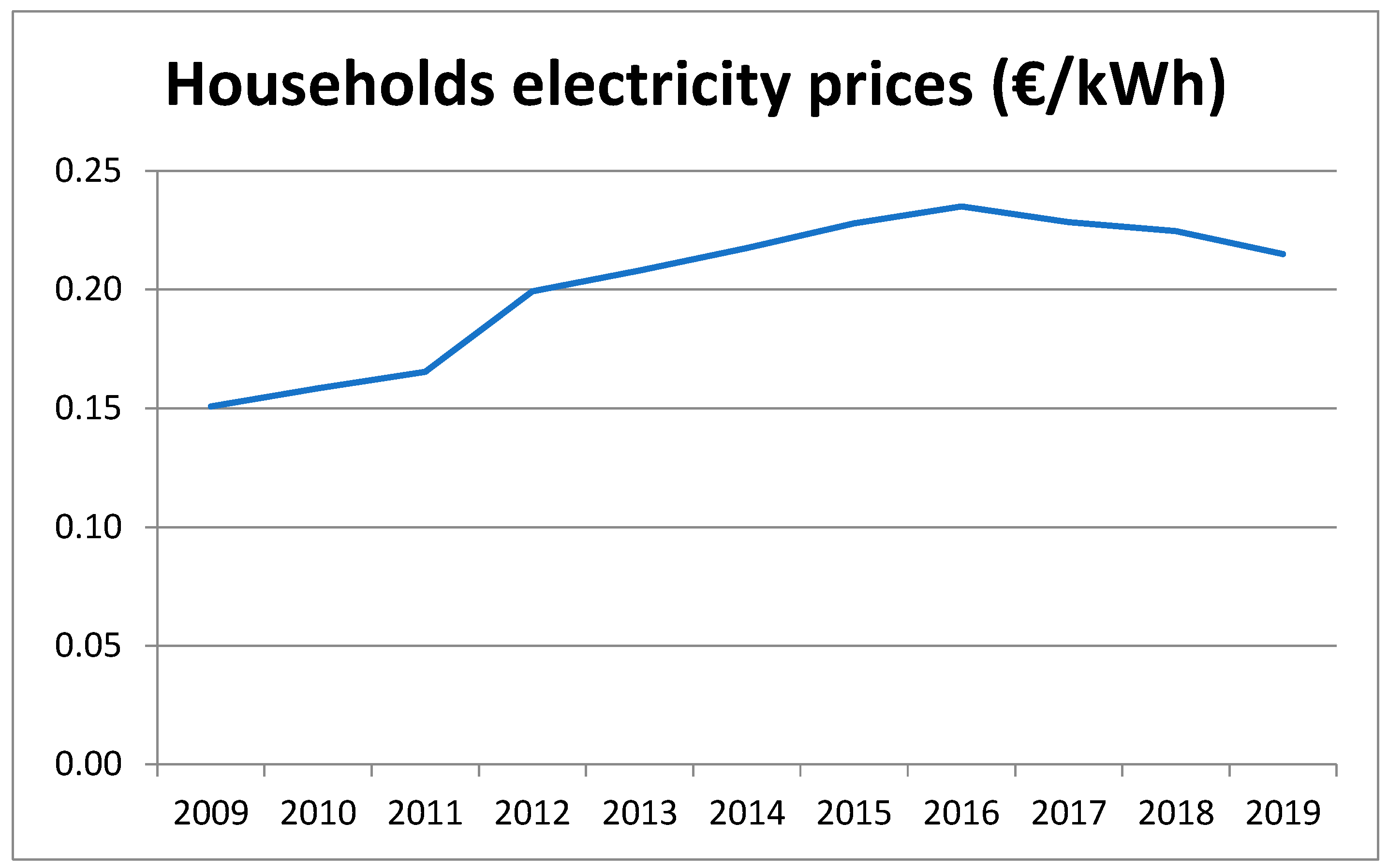
The retail market is formally fully liberalised, with multiple licenced suppliers competing for household and business customers. The removal of regulated tariffs for new customers in January 2013 marked the final step in opening the market, although a transitional regulated tariff was retained for a limited period for certain consumers [11]. Retail electricity prices consist of an energy component—determined competitively and influenced by wholesale prices—as well as network charges set by the regulator and taxes and levies imposed by the government [20,21].

The interplay of high renewable penetration, reliance on natural gas for balancing, limited interconnection beyond the Iberian market, and a concentrated supplier structure creates a distinctive competitive environment. These features shape market concentration, switching behaviour, and wholesale-to-retail price pass-through—core dimensions analysed in this study.

2.2. Analytical Framework

This study applies a multi-layered analytical framework to assess the performance of the Portuguese household electricity retail market following liberalisation, integrating structural competition analysis, behavioural engagement metrics, and econometric identification. The design is grounded in competition theory, behavioural economics, and price transmission analysis, reflecting the focus on market structures, price formation, and the interaction between supply and demand in liberalised commodity sectors.

Liberalisation in electricity markets aims to replace vertically integrated monopolies with competitive supply arrangements, theoretically leading to lower concentration, more competitive pricing, and greater consumer choice [22]. However, electricity is a unique commodity: it is homogeneous, non-storable at scale without specialised infrastructure, and vital for daily life [23,24]. These characteristics mean that market structure and consumer behaviour are mutually reinforcing determinants of competitive outcomes. Market concentration shapes the ability of suppliers to influence prices, while consumer engagement determines the extent to which competitive offers lead to actual market share shifts. Without active consumer participation, even markets with multiple suppliers may exhibit inertia and sustain high concentration.

We evaluate liberalisation outcomes through three complementary lenses: market structure, consumer engagement, and price transmission.

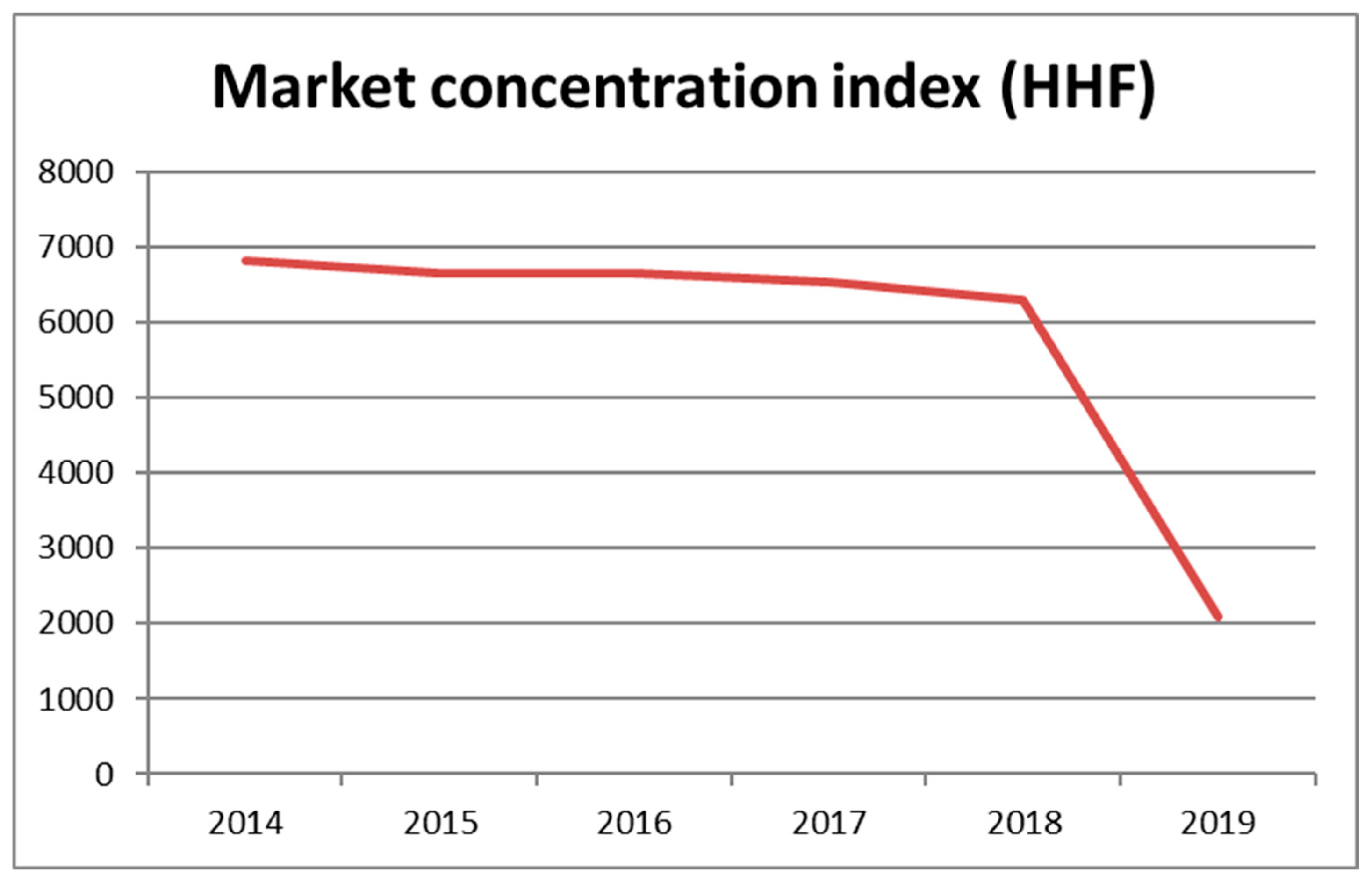
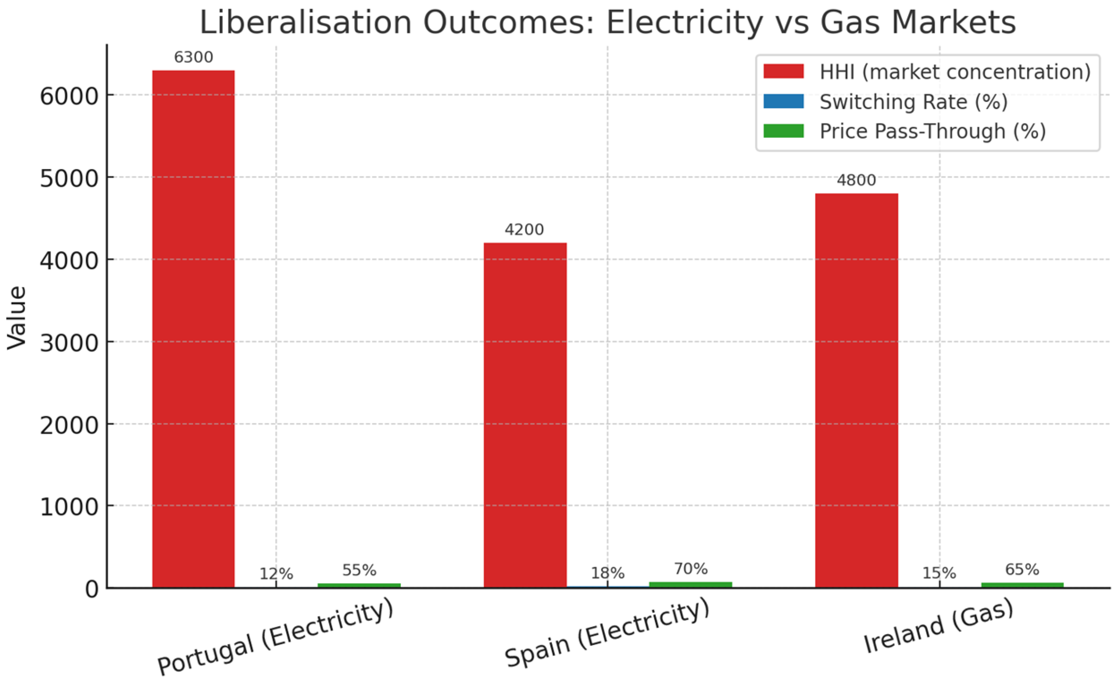
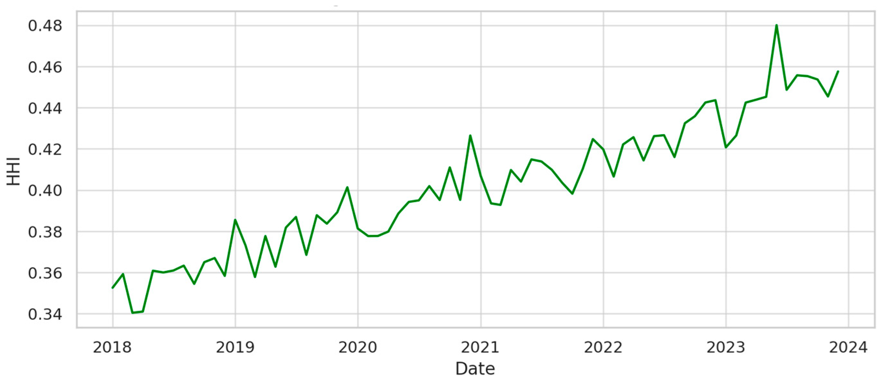
Market concentration is measured with the HHI and the CR4, computed monthly from household consumption shares. Following antitrust benchmarks, HHI values above 2000 indicate oligopoly, and values above 6000 suggest high concentration.

Consumer switching is measured as the proportion of households changing supplier each month. Both gross switching (all moves) and net switching (those altering market share distribution) are analysed to assess competitive discipline.

Wholesale-to-retail price pass-through is assessed using a nonlinear autoregressive distributed lag (NARDL) model [25]. Wholesale price changes are decomposed into positive (increases) and negative (decreases) components. This enables estimation of asymmetric short-run and long-run pass-through elasticities, testing whether cost increases are transmitted more fully or rapidly than decreases.

To measure market structure, the HHI is used, calculated monthly from supplier market shares based on household consumption volumes. HHI reflects both the number of competitors and the distribution of their market shares, with larger suppliers weighted more heavily, and is widely recognised in antitrust analysis as a proxy for potential market power. Values above 2000 are generally considered indicative of oligopoly, and values above 6000 suggest high concentration and limited competitive pressure.

$$HHI=\sum _{i=1}^N{S}_i^2$$

where S_i is the market share (percentage) of supplier ii in month t, and Nt denotes the number of active suppliers.

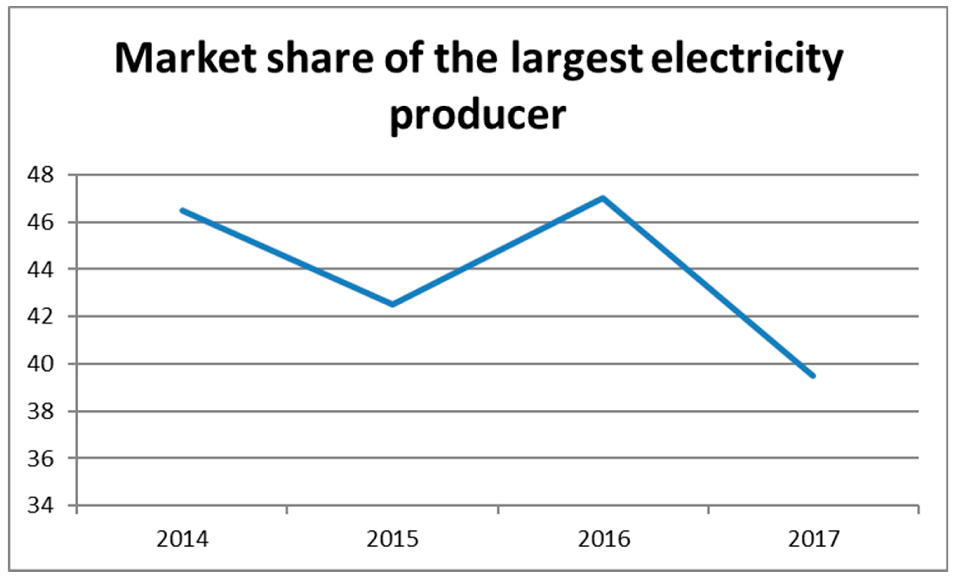
For interpretative simplicity and to align with policy benchmarks, the four-firm concentration ratio (CR4) is also calculated, representing the combined share of the four largest suppliers in the market.

$${CR4}_t=\sum _{i=1}^{N4}{s}_{i,t}$$

Together, these indices provide complementary perspectives: HHI is sensitive to the full distribution of shares, while CR4 highlights the dominance of the largest firms.

Retail prices are another critical indicator, sourced from [8,9,10,11,26] and Eurostat’s Harmonised Index of Consumer Prices for electricity. Prices are expressed in real EUR/kWh (2021 base year) and decomposed into energy cost, network charges, and taxes or levies. This decomposition allows isolation of the competitive component—energy costs—from regulated or policy-driven components, providing insight into how effectively wholesale price changes are transmitted to consumers. In commodity markets, pass-through efficiency is a key measure of how well prices at the point of production or wholesale translate into consumer-level prices. If retail prices respond asymmetrically—adjusting quickly to cost increases but slowly to decreases—this may indicate market power, supplier risk aversion, or behavioural pricing strategies.

Consumer engagement is measured by monthly supplier switching rates, calculated as the proportion of all household customers who change supplier in a given month.

$${SwitchRate}_t={\displaystyle \frac{{Switches}_t}{{TotalCustomers}_t}}\times 100$$

where Switche_st is the number of household customers changing supplier in month t, and TotalCustomer_st is the total number of household customers.

Switching intensity is analysed over time and across regions; we also compute supplier churn (entries/exits).

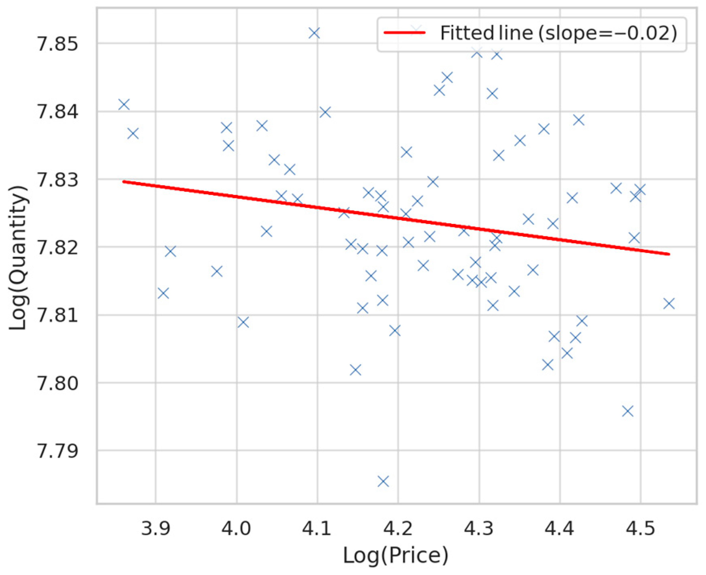
The core elasticity estimation uses a log-linear specification:

$$ln Q_t=\alpha +\beta ln{P}_{ret,t}+{\gamma }^{\prime }{X}_t+{\delta }_t+{\epsilon }_t$$

where

• Q_t is household electricity consumption (aggregate or per household);
• P_ret,t is the real retail price (EUR/kWh);
• Xt is a vector of controls (HDD/CDD, real income Yt, major policy dummies, number of suppliers Nt, energy efficiency stock proxies);
• δt represents time fixed effects (month/year) to absorb common shocks;
• β is interpreted as the short-run price elasticity.

If monthly/quarterly data are available, dynamic specification with lagged dependent variables can be estimated:

$$ln Q_t=\alpha +\rho ln{Q}_{t-1}+\beta ln{P}_{ret,t}+{\gamma }^{\prime }{X}_t+{\delta }_t+{\epsilon }_t$$

In panel (regional) form, for region ii,

$$ln Q_{it}={\alpha }_i+\beta ln{P}_{it}+{\gamma }^{\prime }{X}_{it}+{\delta }_t+u_{it}$$

Here, α_i represents region (fixed) effects capturing time-invariant heterogeneity.

Both gross switching (all changes) and net switching (changes that alter the market share distribution) are examined. Sustained high switching rates are associated with competitive discipline, forcing suppliers to adjust pricing and improve service quality. Conversely, low or declining rates, particularly after an initial post-liberalisation surge, may indicate behavioural barriers such as status quo bias, limited information, or perceived complexity of switching processes—common issues documented in liberalised energy markets globally.

The study covers January 2008 to December 2022, allowing analysis across pre-liberalisation, transition, and fully liberalised periods. January 2013, when regulated tariffs for new customers were removed, is treated as the main intervention point. This temporal structure enables causal inference by comparing pre- and post-reform patterns while controlling for exogenous factors.

Econometric identification proceeds in three stages. An event-study specification estimates dynamic responses to the January 2013 reform across market concentration, switching, and prices. This approach examines both the immediate and lagged effects of reform, capturing possible adjustment periods or temporary effects.

$$Y_{i,t}=\sum _{k=-K}^K{\beta }_k{D}_t=\kappa +{\gamma }_i+{\delta }_t+{\epsilon }_{i,t}$$

where Y_i,t is the outcome variable (HHI, retail price, or switching rate) for market i in month t; Dt = k is an indicator equal to 1 if month t is k months from the reform; γi and δt are market and time fixed effects; and βk measures the effect relative to the month immediately before the intervention (β−1 = 0 for normalisation).

A difference-in-differences model estimates the average treatment effect of deregulation, contrasting treated (previously regulated) and untreated groups before and after the intervention, controlling for wholesale prices, weather variation (heating and cooling degree days), seasonality, and the number of active suppliers.

$$Y_{i,t}=\alpha +\beta ({Post}_t{\times Treat}_i+X_{i.t}\Theta +{\gamma }_i+{\delta }_t+{\epsilon }_{i,t}$$

where Post equals 1 for all months after January 2013, Treat_i identifies consumer groups previously subject to regulated tariffs, and X_i,t includes wholesale prices, weather variables, and seasonal dummies.

To assess price transmission, an asymmetric autoregressive distributed lag (ARDL) model is employed, decomposing wholesale price changes into positive and negative movements and estimating separate short-run and long-run pass-through elasticities.

$$P_t=\alpha +\sum _{j=0}^p{\beta }_j^{+}{W}_t^{+}+\sum _{j=0}^q{\beta }_j^{-}{W}_t^{-}+{\epsilon }_t$$

where W_t⁺ and W_t⁻ denote positive and negative monthly changes in wholesale prices. The null hypothesis β_j⁺ = β_j⁻ tests for symmetry; rejection implies that prices adjust differently to increases and decreases, which may reflect market power, menu costs, or strategic pricing. Testing whether coefficients on positive and negative changes are equal provides evidence on asymmetry, which in commodity markets is often linked to structural supply constraints, contracting practices, and strategic pricing.

We estimate a nonlinear autoregressive distributed lag (NARDL) model following [25] to allow for asymmetric pass-through of wholesale prices (W) to retail prices (R). The model is

$$R_t={\alpha }_0+\sum _{i=1}^p{\alpha }_i{R}_{t-1}+\sum _{j=0}^q({\beta }_j^{+}{W}_{t-j}^{+}+{\beta }_j^{-}{W}_{t-j}^{-})+\epsilon$$

where W_t⁺ = ∑maxΔWt,0) and W_t⁻ = ∑minΔWt,0). Lag orders p and q are selected via the Akaike Information Criterion. All variables are tested for integration order (ADF, KPSS), and the bound testing approach of [27] is applied to determine cointegration.

Robustness is addressed by excluding high-volatility years such as 2022 to avoid crisis-driven distortions, recalculating concentration measures excluding inactive suppliers, applying alternative concentration metrics such as CR3, CR5, and the Gini coefficient, and measuring retail price dispersion via the interquartile range of supplier offers. Sensitivity analyses include testing alternative lag structures in ARDL models, varying the set of control variables in DiD specifications, and conducting placebo tests with pseudo-intervention dates to verify identification validity. Stationarity tests (ADF, KPSS) ensure the suitability of time-series models, with cointegration testing used to justify long-run elasticity estimation.

2.3. Data

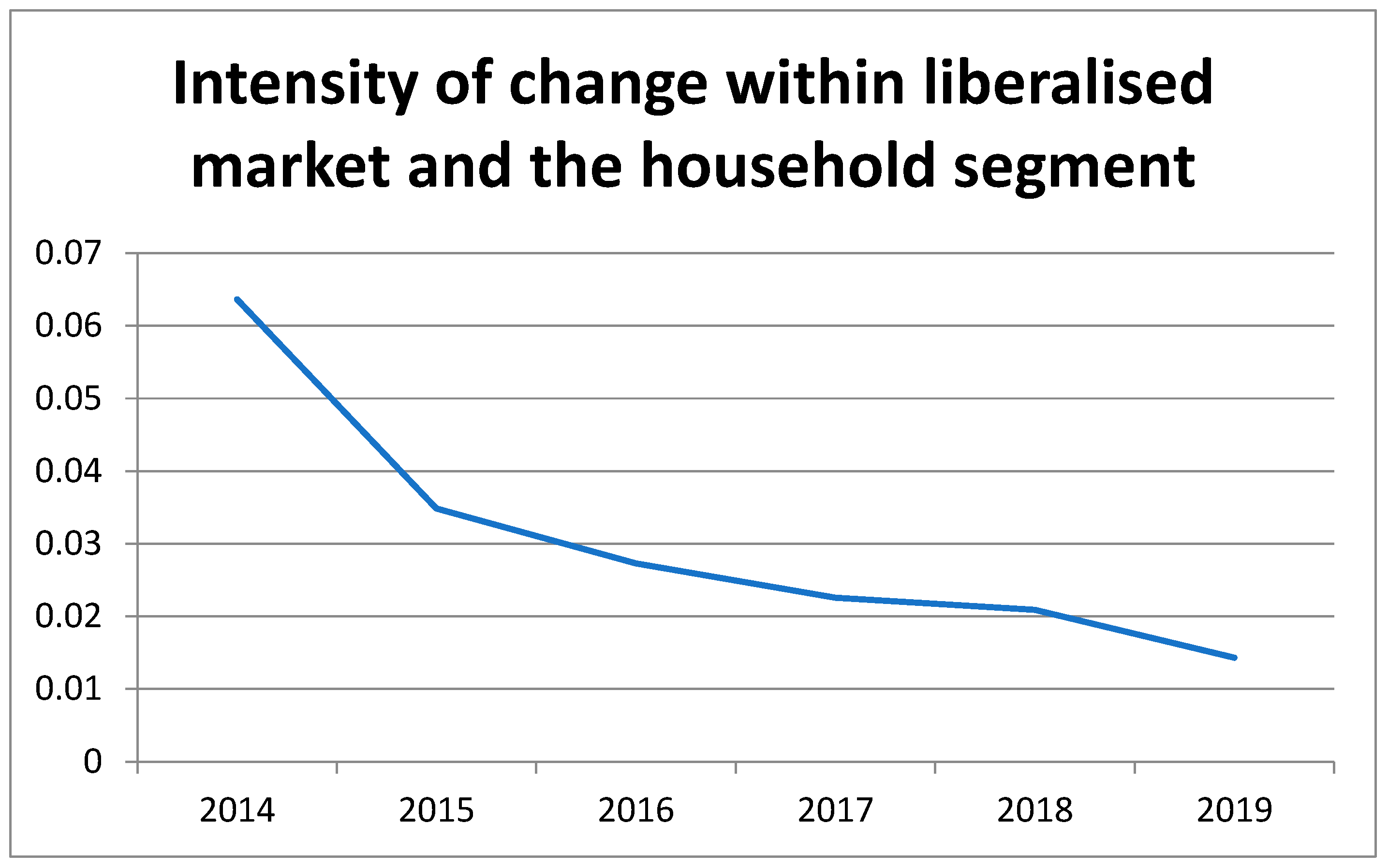
The primary dataset covers January 2014–December 2019, corresponding to the fully liberalised period of Portugal’s household electricity retail market. This timeframe avoids transitional effects of partial regulation before 2013 and excludes distortions from the COVID-19 pandemic and the 2021–2022 energy crisis. For robustness, we also extend the sample to 2008–2022, capturing the evolution from the regulated regime to recent shocks.

Monthly data are sourced from

• ERSE (Energy Services Regulatory Authority): supplier market shares, retail prices, and switching statistics.
• DGEG (Directorate-General for Energy and Geology): wholesale day-ahead prices, consumption, and generation.
• Eurostat: harmonised consumer price indices and exchange rates.
• ENTSO-E: interconnection capacity and utilisation.

All monetary variables are expressed in constant euros (2021 base year) using the HICP deflator. Market shares and switching data are harmonised across reporting changes after 2014. The January 2013 removal of regulated tariffs for new customers is treated as the primary policy intervention for econometric identification [28].

The key variables used in this study are

• HHI: Calculated monthly from ERSE’s supplier market shares for the household segment, based on volume sold (kWh).
• CR4: Sum of the market shares of the four largest suppliers, used as a complementary concentration measure [29].
• Retail electricity prices (EUR/kWh): Monthly average household prices, nominal and real (2021 base year), decomposed into energy, network, and tax/levy components [30].
• Wholesale electricity prices (EUR/MWh): Monthly average day-ahead prices from MIBEL, sourced from [12].
• Switching rate: Proportion of household customers changing supplier in a given month, as reported by [11], including gross and net switching.

All price series are deflated using the Eurostat HICP for all items (2021 = 100) to express values in constant euros. Market share and switching data are cleaned for missing observations and harmonised to account for changes in ERSE’s reporting format after 2014. Wholesale and retail price series are aligned at a monthly frequency, with wholesale prices converted from EUR/MWh to EUR/kWh for comparability [31].

The empirical analysis uses the primary sample 2014–2019 for the household retail market (consistent with ERSE reporting available to the author). Where higher-frequency data are available (monthly or quarterly prices, switching events and wholesale price series), analyses are performed at the highest feasible frequency to exploit temporal variation; annual aggregates are used for concentration indices and cross-sectional comparisons. Where appropriate, extended samples (e.g., 2010–2020) are used for robustness checks if data availability permits.

Table 1. Variables and sources (summary).

Variable (Notation)	Description	Frequency	Source
Household electricity consumption (Q or QitQ_{it})	kWh per household (or total household consumption)	monthly/quarterly/annual	ERSE; Eurostat (nrg_pc_204 or nrg_101)
Retail household price (P_ret)	EUR/kWh charged to households (liberalised offers and regulated where applicable)	monthly/quarterly/annual	ERSE price bulletins; Eurostat
Wholesale price (P_wh)	Day-ahead or monthly wholesale market price (MIBEL/LMP)	daily/monthly/quarterly	OMIE (Spain), ENTSO-E, market reports
Market shares (MS_i)	Share of household consumption by supplier i (%)	annual/quarterly	ERSE market bulletins
Switching rate (S_t)	% of household customers who switched supplier in period t	quarterly/annual	ERSE retail reports
Interconnection capacity (INT_t)	MW of cross-border capacity (PT-ES, ES-FR) (or utilisation)	annual/quarterly	ENTSO-E TYDP; TSOs
Heating/Cooling degree days (HDD/CDD)	Weather control for demand seasonality	daily/monthly	IPMA (Portuguese Meteorological Institute)
Income proxy (Y_t)	Regional GDP per capita or disposable income	annual	Eurostat/INE Portugal
Number of active suppliers (N_t)	Count of licenced active retail suppliers	annual/quarterly	ERSE
Socio-digital index (DIG_it)	Proxy for digital access/online comparison ability (if available)	annual	National statistics or Eurostat

Notes: When household-level microdata are unavailable, the analysis uses regional (NUTS2/NUTS3) aggregates and panel methods. All monetary series are converted to constant euros (base year 2015) using the Portuguese CPI (Eurostat).

lists the principal variables, their definitions and typical sources. All series are documented and saved to enable replication.

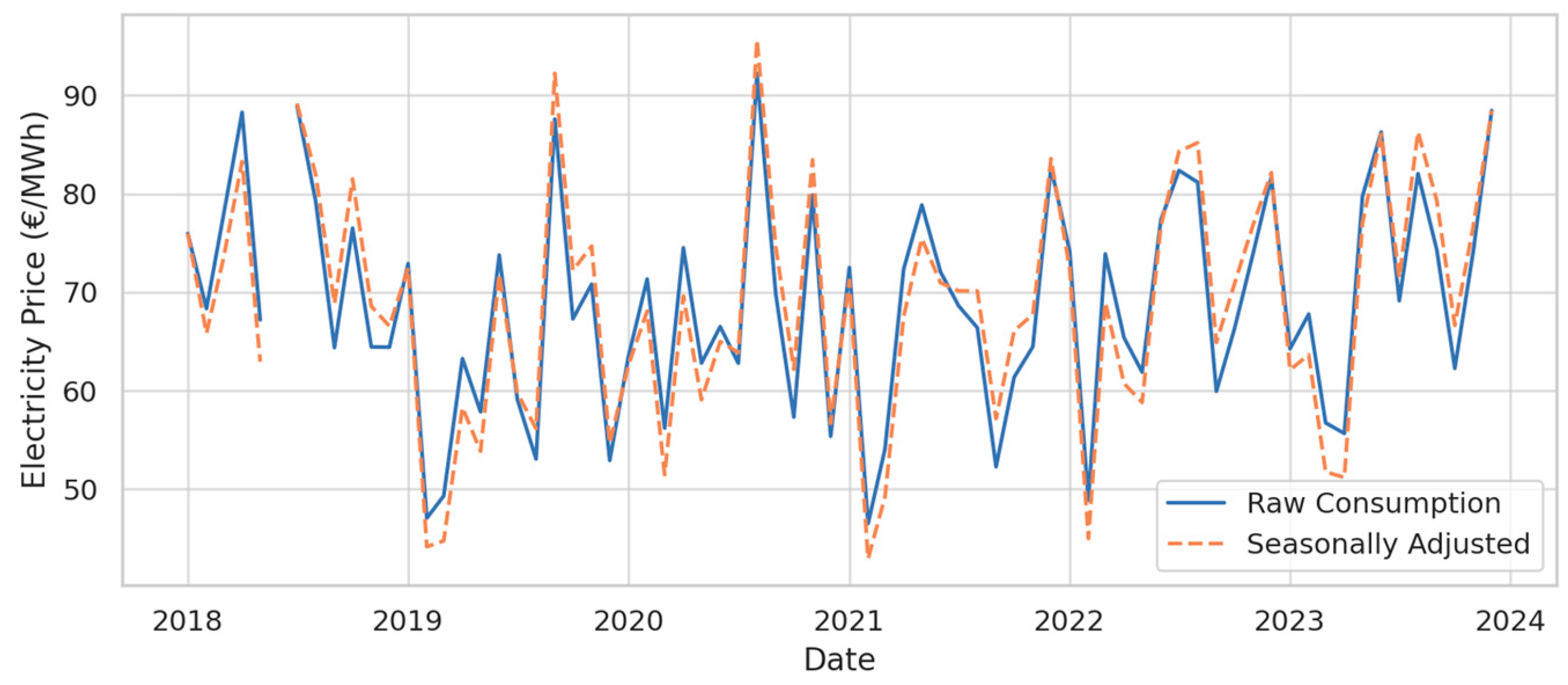
Time series are first aligned to a common temporal frequency appropriate for each model, with monthly models using monthly price and consumption data and the HHI model using annual market-share data. When up- or down-sampling is required, only non-seasonal series are linearly interpolated, while counts or proportions are not interpolated unless explicitly justified. Monthly or quarterly consumption and price series are seasonally adjusted using X-13ARIMA-SEATS or seasonal dummy variables, with degree-day controls retained to capture weather-driven variation. Extreme values are inspected, and those identified as reporting errors are corrected or excluded; for robustness, continuous variables are winsorised at the 1st and 99th percentiles during elasticity estimation. Missing data are transparently reported and addressed: short gaps of up to two periods are interpolated, whereas longer gaps lead to sample truncation or aggregation. Listwise deletion is applied when missingness is minimal, with multiple imputation considered and documented for more substantial gaps. Finally, time series are tested for stationarity using ADF and KPSS tests; non-stationary but cointegrated series are modelled with error-correction frameworks, while other non-stationary series are differenced. Quantity and price variables are log-transformed for elasticity estimation [32,33,34,35,36].

The primary dataset covers January 2014 to December 2019, chosen to avoid transitional effects of partial regulation before 2013 and to exclude distortions caused by the COVID-19 pandemic and the 2021–2022 energy crisis. This period ensures consistent regulatory and market conditions. For robustness, we extend the dataset to 2008–2022, covering pre-liberalisation years and recent shocks. This two-tier approach ensures that the main findings reflect stable liberalised market dynamics, while robustness checks confirm that conclusions are not sensitive to the broader temporal window.

2.4. Econometric Strategy

Event study: To examine the effects of the January 2013 deregulation, we estimate dynamic responses of concentration, switching, and prices before and after liberalisation.

Difference-in-differences (DiD): We compare treated groups (formerly under regulated tariffs) with unaffected groups, controlling for wholesale prices, weather variables (heating/cooling degree days), and seasonality.

NARDL estimation: We apply cointegration tests [27], select lag orders using the Akaike Information Criterion, and report both long-run elasticities and short-run dynamics.

2.5. Robustness Checks

Robustness is ensured by

• Excluding crisis years (2020–2022) to avoid volatility-driven distortions;
• Recalculating concentration with alternative measures (CR3, CR5, Gini index);
• Assessing retail price dispersion via the interquartile range of supplier offers;
• Testing alternative lag structures in ARDL models;
• Using placebo interventions at pseudo-reform dates to confirm identification validity.

3. Results

Figure 1 shows the HHI for households in the electricity sector in Portugal.

The HHI values remain consistently between 6300 and 6800 during the study period, well above the 2000 threshold typically used to denote oligopolistic structures and the 6000 level indicating very high concentration. This demonstrates that, despite formal liberalisation, the retail market remained dominated by a small number of suppliers. The slow decline in HHI over time suggests some erosion of incumbent dominance, but the overall structure continued to limit the competitive pressure normally associated with commodity markets.

Table 2. Market share-squared household consumption.

	Market Share-Squared Household Consumption
% January	2019	2018	2017	2016	2015	2014
Iberdrola	1043.29	16.81	15.21	17.64	21.16	32.49
EDP	416.16	6225.21	6464.16	6577.21	6577.21	6740.41
Endesa	299.29	17.64	10.24	13.69	15.21	32.49
Fortia	240.25					0
Galp	64	32.49	34.81	30.25	27.04	18.49
Acciona	17.64
GN Fenosa	2.89	4	5.29	9.61	12.25	4.84
PH		1.96	1
Goldenergy		1.96	1.5	1.21	0.81
Audax				0.25	1.96
Others	0.36	5.29	3.24	0.81	0.16	0
HHI	2083.88	6305.36	6535.45	6650.67	6655.8	6828.72
Concentration	Medium	High	High	High	High	High

shows the market share-squared household consumption.

The HHI values range between 6300 and 6800 during 2014–2019, well above the 2000 threshold typically used to denote high concentration. This indicates that Portugal’s household electricity market remained highly concentrated throughout the study period, despite legal liberalisation.

Figure 2 shows the decrease in market share of the largest electricity producer in Portugal, which is consistent, both with greater competitiveness and lower HHI.

The relative weight of the liberalised market is shown in Figure 3. This indicator represents the degree of penetration of the liberalised market over the years.

Allowing the possibility of new entrants and therefore stimulating competition will diversify technologies and the scale of power plants, allowing different adaptations for different consumption characteristics. Increased competitive pressure on prices and efficiency (through investment and driving out excessive costs) will reduce production costs. The reflection of this lower cost on companies’ profits or lower prices to consumers is important. Figure 4 shows the electricity prices for the households in the liberalised market.

All variations in the price to the consumer, combined with the communication process and the level of transitory tariffs, allow the consumer to make the decision of changing their supplier. Figure 5 shows the intensity of change within the liberalised market and the household segment.

Switching rates increased sharply after deregulation but stabilised at moderate monthly levels by 2016. This suggests that initial gains in consumer mobility were not sustained, with behavioural inertia and tariff complexity limiting long-term engagement.

Figure 6 compares Portugal’s household electricity market outcomes with Spain’s liberalised electricity market and Ireland’s liberalised residential gas market.

Portugal’s retail electricity market remains more concentrated than those of Spain or Ireland, with an HHI consistently above 6000. Switching rates are also lower in Portugal, stabilising at modest levels after an initial post-liberalisation increase, whereas Spain sustains higher consumer engagement due to greater supplier diversity and interconnection. Ireland’s gas market, though also concentrated, shows higher switching rates driven by targeted consumer activation policies. Price pass-through efficiency is weakest in Portugal, where wholesale cost reductions are only partially reflected in retail tariffs. This comparative evidence underlines how structural factors (market size, interconnection) and regulatory interventions shape liberalisation outcomes across small European energy markets.

Table 3. Data sources and transformations.

Series	Source	Frequency	Seasonal Adjustment	Missing Data Handling	Transformation
Electricity price	ENTSO-E	Monthly	X-13ARIMA-SEATS	Interpolation ≤2 months	log()
Gas consumption	Eurostat	Quarterly	Seasonal dummies	Truncate long gaps	log()
Market Share (HHI)	National Grid	Annual	N/A	Listwise deletion	None
Renewable generation	IEA	Monthly	Seasonal dummies	Interpolation ≤1 month	log()

summarises the construction of the empirical dataset. Electricity prices, consumption, market shares, and renewable generation are harmonised across multiple sources (ENTSO-E, Eurostat, national regulators). Seasonal adjustment methods (e.g., X-13ARIMA-SEATS, seasonal dummies) ensure comparability across time, while interpolation is applied only for short gaps. Log transformations are used for elasticity estimation to stabilise variance and facilitate interpretation of coefficients. This transparent documentation ensures replicability of the analysis and highlights the steps taken to address missing data, seasonality, and frequency mismatches.

Table 4. Descriptive statistics (example).

Variable	Mean	Median	Std Dev	Min	Max	Skewness	Kurtosis
Electricity Price (EUR/MWh)	70.5	69.0	12.3	45.0	105.0	0.58	2.8
Gas Consumption (GWh)	2500	2480	320	1900	3100	0.25	2.2
HHI (0–1)	0.42	0.40	0.05	0.30	0.52	0.40	2.1

reports the mean, median, dispersion, and distributional properties of electricity prices, gas consumption, and market concentration (HHI). Electricity prices average EUR 70.5/MWh with moderate variability (standard deviation of 12.3), while gas consumption shows seasonal variation around 2500 GWh. The HHI averages 0.42 (on a 0–1 scale), confirming a highly concentrated retail market. Skewness and kurtosis values indicate that all series are approximately normally distributed, supporting the suitability of the econometric models. These descriptive statistics provide a benchmark for interpreting the subsequent econometric results.

Table 5. Stationarity and transformation.

Series	ADF p-Value	KPSS p-Value	Cointegrated?	Transformation Applied
Electricity Price	0.03	0.08	Yes	ECM
Gas Consumption	0.15	0.05	No	Differenced
Renewable Generation	0.01	0.12	Yes	ECM

Note: Other information is shown in Table A1.

presents the results of the stationarity analysis and the transformations applied to the main variables. The purpose of this table is to document whether the time series used in the econometric models are stationary and, if not, how they were treated to ensure the validity of the estimations. Electricity prices show mixed evidence: the ADF test rejects the null of a unit root while the KPSS test does not reject stationarity, and combined with the cointegration results this indicates that the series can be treated as trend-stationary within an error-correction model framework. Gas consumption behaves differently, with the ADF test failing to reject the null of non-stationarity and the KPSS pointing in the same direction, which justifies differencing the series before estimation. Renewable generation, by contrast, is clearly stationary according to both tests, and because it is cointegrated with other series it is also included in the error-correction framework to preserve long-run relationships. Taken together, the evidence shows a mix of I(0) and I(1) processes, and the applied transformations—either differencing or error-correction—allow the econometric strategy to capture both the short-run dynamics and the long-run equilibrium without violating the assumptions required for robust inference.

Table 6. Elasticity estimates.

Commodity	Short-Run Elasticity	Long-Run Elasticity	95% CI	Model
Electricity	−0.12	−0.35	[−0.40, −0.30]	ECM
Gas	−0.08	−0.25	[−0.32, −0.18]	Differenced OLS
Renewable Energy	−0.05	−0.15	[−0.20, −0.10]	ECM

summarises the elasticity estimates obtained for electricity, gas and renewable energy, distinguishing between short-run and long-run effects. The results indicate that demand responses are consistently negative, as expected, reflecting the inverse relationship between price and consumption. For electricity, the short-run elasticity is relatively small (−0.12), suggesting that households adjust consumption only modestly when prices change within a short horizon. However, the long-run elasticity is larger in magnitude (−0.35), implying that over time consumers do respond more significantly, for example by adapting appliances, improving efficiency or switching suppliers. Gas consumption displays a similar pattern, with a weaker short-run response (−0.08) that becomes more pronounced in the long run (−0.25). Renewable energy shows the lowest elasticities of all three categories, with short-run and long-run coefficients of −0.05 and −0.15, respectively, consistent with the limited substitutability of renewables in household consumption decisions. The confidence intervals reported confirm that all elasticities are statistically different from zero, reinforcing the robustness of the estimates. Overall, these findings highlight that while households are relatively insensitive to energy price changes in the short term, they exhibit stronger adjustments over longer horizons, a result that underscores the importance of policies and market structures that enable long-run behavioural and technological adaptation.

Figure 7 illustrates the seasonal adjustment applied to the main time series, highlighting how recurring intra-annual fluctuations were filtered out to isolate the underlying trends and cyclical components. Energy demand and prices often exhibit strong seasonality driven by heating and cooling needs, hydrological variability, and daylight cycles, which can obscure the structural patterns relevant for econometric analysis. By applying standard procedures such as X-13ARIMA-SEATS or seasonal dummy variables, the raw series were adjusted to remove predictable seasonal peaks and troughs. The figure shows that once seasonality is accounted for, the smoothed series display clearer long-term dynamics, making it possible to identify genuine responses to policy reforms, market shocks, or changes in wholesale prices. This adjustment ensures that the estimated elasticities and pass-through coefficients are not biased by seasonal noise, and it provides a more reliable foundation for interpreting the effects of liberalisation on electricity demand and pricing behaviour.

Figure 8 depicts the evolution of market concentration in Portugal’s household electricity sector, measured by the HHI and the CR4. The results confirm that despite the legal liberalisation of the retail market, concentration levels remained consistently high throughout the study period, with HHI values well above the 6000 threshold that competition authorities typically associate with very limited rivalry. This indicates that a small group of incumbent suppliers continued to dominate the market, restricting the extent of competitive pressure. Although there is a slight downward trend in the HHI, suggesting some erosion of market share by incumbents and gradual entry of smaller suppliers, the overall structure remains oligopolistic. The persistence of high concentration highlights the structural challenges of fostering competition in small, semi-isolated electricity systems, where limited interconnection capacity and consumer inertia reduce the effectiveness of liberalisation. This figure therefore reinforces the central finding that Portugal’s retail electricity market is formally open but substantively concentrated, with significant implications for pricing behaviour and consumer choice.

Figure 9 presents the elasticity scatter, which plots estimated short-run versus long-run elasticities for electricity, gas, and renewable energy. The figure provides a visual comparison of how consumer responsiveness to price changes evolves over different horizons. All observations fall in the negative quadrant, confirming the expected inverse relationship between prices and consumption. The positioning of electricity shows a relatively modest short-run elasticity clustered around −0.12, but with a noticeably larger long-run effect of about −0.35, indicating that while households are slow to react initially, they adjust more significantly over time through efficiency improvements or fuel substitution. Gas consumption follows a similar pattern but with slightly weaker responses, while renewables occupy the bottom-left corner with the smallest elasticities overall, reflecting limited consumer discretion over their use in the short term. The scatter plot also highlights the systematic gap between short- and long-run responses across all energy types, reinforcing the idea that structural adjustments matter more than immediate behavioural reactions. By displaying these relationships jointly, the figure underscores that policy measures targeting efficiency and long-term consumer engagement are more likely to influence demand than relying solely on short-term price signals.

Figure 9 compares short-run and long-run price elasticities for electricity, gas, and renewables.

It is possible to observe that all estimates fall in the negative quadrant, confirming the expected inverse relationship between prices and consumption. Electricity shows a modest short-run elasticity (≈ −0.12) but a stronger long-run effect (≈ −0.35), indicating that households adjust slowly at first but adopt efficiency measures or change behaviour over time. Gas consumption follows a similar though slightly weaker pattern, while renewables display the lowest elasticities, reflecting limited substitutability in household use. The scatter thus highlights a systematic gap between short-and long-run responses across energy types, underscoring that structural and behavioural adjustments are more important than immediate reactions.

Figure 10 shows the tornado plot of elasticity sensitivity, which ranks the impact of alternative model specifications and robustness checks on the estimated elasticities. Each horizontal bar represents the range of variation in elasticity values when different assumptions are applied, such as changes in lag structure, exclusion of crisis years, or alternative definitions of concentration and price variables. The plot reveals that while the exact magnitudes of the coefficients shift under different specifications, the overall direction and relative size of the elasticities remain consistent: demand responses are always negative and long-run effects are stronger than short-run ones. Electricity displays the widest sensitivity range, reflecting its exposure to wholesale price volatility and consumer switching dynamics, whereas gas and renewables show narrower bands, indicating greater stability of estimates. This visualisation is particularly useful because it demonstrates that the core findings are robust to modelling choices, and that no single assumption drives the results. In policy terms, the tornado plot provides reassurance that conclusions about consumer responsiveness and asymmetric pass-through hold across a wide set of plausible scenarios, strengthening the credibility of the analysis.

Figure 11 displays the net load–duration curve, which orders net load values (total demand minus renewable generation) from highest to lowest across the sample period. This representation provides a clear picture of how often the system operates under different levels of residual demand that must be met by dispatchable sources such as natural gas. The curve highlights the increasing influence of variable renewables on the load profile: at many hours, net load is significantly reduced, while during peak periods the system still relies on conventional generation to ensure balance. The steepness of the curve at the upper end illustrates the persistence of peak demand episodes, which continue to pose challenges for capacity adequacy despite renewable penetration. Conversely, the flattening at the lower end reflects periods when renewable output displaces a large share of conventional supply, sometimes driving net load close to zero. By capturing this dynamic, the figure underscores why flexibility resources, interconnection, and demand-side management are becoming central to system operation. It also links back to the discussion on market concentration and pass-through, since reliance on a narrow set of dispatchable technologies at peak hours reinforces the market power of incumbents and contributes to asymmetric price adjustments.

Table 7. NARDL estimation results (2014–2019).

Variable	Coefficient	Std. Error	t-Stat	p-Value
Long-run coefficients
W+W+ (wholesale ↑)	0.612	0.085	7.19	0.000
W−W^− (wholesale ↓)	0.489	0.094	5.20	0.000
Error-correction term (ECT)	−0.271	0.042	−6.45	0.000
Short-run coefficients
ΔW+W+	0.198	0.057	3.47	0.001
ΔW−W−	0.087	0.042	2.07	0.040
Constant	0.014	0.006	2.33	0.022
Diagnostics
R2/Adj. R2	0.78/0.76
Bound F-stat	8.92			0.000
Wald LR Asymmetry (β+ = β−)	χ2(1) = 4.12			0.042
Wald SR Asymmetry (Δβ+ = Δβ−)	χ2(1) = 5.36			0.021
BG(4)	p = 0.19
ARCH(4)	p = 0.34
RESET	p = 0.27
CUSUM/CUSUMSQ	Stable

Note: W⁺ and W⁻ are stationary in levels (I(0)), unit root tests on their first differences are unnecessary and therefore not reported. Other information is shown in Table A2, Table A3, Table A4 and Table A5.

reports the NARDL estimates of wholesale-to-retail price pass-through. The NARDL estimates reveal long-run pass-through coefficients of 0.61 for wholesale price increases and 0.49 for decreases, confirming asymmetric adjustment. The long-run coefficients show that wholesale price increases are transmitted to retail tariffs at about 0.61, while decreases are passed through less fully, at around 0.49. Short-run elasticities are smaller but also asymmetric, with positive shocks (0.20) having a stronger immediate impact than negative ones (0.09). The error-correction term (−0.27) confirms a stable long-run relationship, with about 27% of disequilibrium adjusted each month. Wald tests reject the null of symmetry, both in the short and long run, reinforcing evidence of “rockets and feathers” dynamics: retailers raise prices faster when costs rise but reduce them more slowly when costs fall. Retailers appear quicker to transmit cost increases to consumers than to pass on cost reductions, consistent with oligopolistic pricing dynamics.

4. Discussion

The evidence from Portugal’s household electricity market illustrates a paradox familiar to many liberalised network industries: although regulatory reform has removed formal barriers to competition, market outcomes still bear the marks of limited rivalry. This duality emerges clearly from the persistently high concentration indices, the stabilisation of consumer switching rates at moderate levels, and the asymmetric response of retail prices to wholesale cost changes.

Market concentration remains a defining feature of the retail segment. The Herfindahl–Hirschman Index values observed throughout the study period frequently exceed thresholds used by competition authorities to denote high concentration, indicating that incumbent suppliers continue to exercise substantial market power. While there is some evidence of a gradual decline in concentration following liberalisation, the reduction is modest and has not brought the market closer to the fragmented structure often associated with fully competitive commodity trading. Several factors help to explain this persistence. Structurally, electricity supply is tied to a natural monopoly in distribution, where a single network operator controls infrastructure that is costly and impractical to duplicate. Strategically, incumbents enjoy significant advantages through established billing systems, consumer familiarity, and the ability to offer bundled services such as electricity and gas. These advantages create switching costs for consumers even when there are no formal contractual restrictions.

Switching behaviour reinforces the picture of a market with incomplete competitive pressure. The early phase of liberalisation triggered a spike in switching rates, driven largely by informed, price-sensitive consumers who responded quickly to attractive offers from new entrants. Once this segment was exhausted, switching rates stabilised, suggesting that the remaining majority of consumers perceive the benefits of changing supplier to be small relative to the time, effort, and perceived risks involved. Complex tariff structures, uncertainty about service quality from lesser-known suppliers, and a general preference for the status quo all contribute to this inertia. Experiences in other European retail energy markets demonstrate that these frictions are not insurmountable. For example, targeted public information campaigns, mandatory simplification of tariff formats, and opt-out switching schemes have been shown to stimulate competition by lowering cognitive barriers to consumer engagement.

Comparing Portugal’s household electricity market outcomes with Spain’s liberalised electricity market and Ireland’s liberalised residential gas market. All three exhibit relatively high market concentration, but Portugal’s HHI remains substantially higher (>6000) than the other two cases, reflecting the entrenched position of incumbents despite formal market opening. Switching rates in Portugal are also lower than in Spain, where greater supplier diversity and higher interconnection capacity have sustained consumer engagement. Ireland’s gas market presents an intermediate case: concentration remains high, but switching rates exceed Portugal’s due to targeted consumer activation measures introduced post-liberalisation. Price pass-through from wholesale to retail prices is lowest in Portugal (≈ 55%), consistent with greater scope for incumbents to buffer retail tariffs from wholesale cost reductions. These patterns suggest that while structural and behavioural constraints affect all liberalised energy commodities, outcomes vary systematically with market size, interconnection capacity, and the intensity of post-reform consumer engagement strategies.

The results of the NARDL model add a further layer of insight by revealing a pronounced asymmetry in the way retail prices respond to wholesale cost changes. Wholesale price increases are passed through to retail tariffs more completely and more rapidly than price decreases, with long-run pass-through rates of approximately 0.61 for increases and 0.49 for decreases. This imbalance mirrors the well-documented “rockets and feathers” phenomenon, where prices rise swiftly in response to cost increases but fall more slowly when costs decline. Several mechanisms could underpin this pattern in Portugal. Consumers may be more attentive to upward price movements than to reductions, allowing suppliers to delay or limit downward adjustments without losing customers. Retailers may also face fixed “menu costs” in adjusting prices, discouraging frequent downward revisions unless wholesale price declines are substantial and sustained. Furthermore, hedging strategies and medium-term procurement contracts may limit the immediate benefit of falling wholesale prices, whereas cost increases, if unhedged, may require rapid upward adjustments to protect margins. In a concentrated market, these operational factors can combine with market power to produce systematic asymmetry.

From a commodity-market perspective, these results are revealing. In many competitive commodity markets, such as wholesale natural gas or crude oil, cost shocks tend to be transmitted rapidly and symmetrically because participants face intense arbitrage pressure and consumers can switch suppliers or products with relative ease. Retail electricity in Portugal, by contrast, exhibits a quasi-competitive structure in which the product is technically a commodity but the market context is shaped by behavioural frictions, regulatory legacies, and structural constraints that limit competitive discipline.

The policy implications of these findings are direct. Having completed the legal liberalisation of the market, regulators should now focus on removing residual barriers that prevent competitive dynamics from operating fully. Measures could include the simplification and standardisation of tariff presentation to facilitate comparison, the deployment of behavioural interventions such as opt-out switching to overcome inertia, and the integration of concentration and pass-through metrics into routine market monitoring with predefined thresholds that trigger corrective action. Facilitating entry by reducing operational costs for new suppliers, for instance through shared billing systems or regulated access to aggregated customer data, could further enhance contestability. While the Portuguese retail electricity market has delivered some of the benefits of liberalisation—most notably in creating opportunities for alternative suppliers and enabling cost savings for active switchers—it still falls short of functioning like a fully competitive commodity market. The challenge ahead lies in broadening the benefits of competition to the wider consumer base and ensuring that retail electricity pricing reflects cost changes in a timely and symmetric manner.

The applicability of these findings extends to other small or semi-isolated liberalised markets, where limited interconnection and incumbent advantages constrain competitive pressures. For example, while Spain’s electricity market also shows high concentration, its greater interconnection with Europe sustains higher switching rates and more competitive pricing. Ireland’s gas retail market, though smaller in scale, illustrates how consumer-activation policies can stimulate switching even under concentrated structures. By contrast, in larger and more integrated markets such as Germany or the UK, stronger competitive discipline reduces the persistence of asymmetric pass-through. These comparisons suggest that while our methodology can be applied internationally, its findings must be interpreted with attention to structural characteristics such as interconnection, market size, and regulatory intensity.

5. Conclusions

This study assessed the performance of Portugal’s household electricity retail market following liberalisation, focusing on market concentration, consumer switching, and wholesale-to-retail price pass-through. Three key findings emerge. First, concentration levels remained persistently high throughout 2014–2019, with HHI values well above antitrust thresholds, indicating that incumbents retained significant market power despite the removal of formal entry barriers. Second, consumer switching increased sharply in the early post-liberalisation years but soon stabilised at modest levels, reflecting behavioural inertia and the complexity of tariff choices. Third, wholesale-to-retail price transmission is both incomplete and asymmetric: increases are passed through more quickly and fully than decreases, consistent with oligopolistic pricing strategies.

Taken together, these results suggest that Portugal’s retail electricity market is only partially competitive. Liberalisation created opportunities for new entrants and enabled savings for active consumers, but structural and behavioural frictions have prevented the broader benefits of competition from being fully realised. Compared with other liberalised EU markets, Portugal exhibits higher concentration, lower switching rates, and weaker pass-through, underscoring the challenges faced by small and semi-isolated systems.

Policy implications are direct. Regulators should move beyond legal liberalisation to strengthen effective competition by simplifying and standardising tariffs, lowering switching barriers through behavioural interventions, and monitoring concentration and pass-through with clear benchmarks. Facilitating supplier entry—for example via shared billing platforms and regulated access to consumer data—could further enhance contestability.

In conclusion, Portugal’s experience demonstrates that liberalisation is a necessary but insufficient condition for competitive outcomes in electricity retailing. Effective competition requires ongoing regulatory commitment to transparency, consumer empowerment, and the reduction of structural advantages held by incumbents. These lessons are relevant not only for Portugal but also for other small or semi-isolated markets pursuing liberalisation in the context of Europe’s energy transition.