Article

Commodity Spillovers and Risk Hedging: The Evolving Role of Gold and Oil in the Indian Stock Market

by
Narayana Maharana
1,*,
Ashok Kumar Panigrahi
2,* and
Suman Kalyan Chaudhury
3
1
Department of Management Studies, Gayatri Vidya Parishad College of Engineering, Kommadi, Visakhapatnam 530048, Andhra Pradesh, India
2
Department of Technology Management, NMIMS University, Shirpur 425405, Maharashtra, India
3
Department of Business Administration, Berhampur University, Bhanja Bihar, Berhampur 761110, Odisha, India
*
Authors to whom correspondence should be addressed.
Commodities 2025, 4(2), 5; https://doi.org/10.3390/commodities4020005
Submission received: 31 January 2025 / Revised: 22 March 2025 / Accepted: 1 April 2025 / Published: 8 April 2025

Abstract

:
This study examines the volatility and hedging effectiveness of commodities, specifically gold and oil, on the Indian stock market, focusing on both aggregate and sectoral indices. Data have been collected from 1 January 2021 to 31 December 2024 to cover the post-COVID-19 period. Utilizing the Asymmetric Dynamic Conditional Correlation Generalized Autoregressive Conditional Heteroskedasticity (ADCC-GARCH) model, we analyze the volatility spillovers and time-varying correlations between commodity and stock market returns. The analysis of spillover connectedness reveals that both commodities exhibit limited and inconsistent hedging potential. Gold demonstrates low and stable spillovers in most sectors, indicating its diminished role as a reliable safe-haven asset in Indian markets. Oil shows relatively higher but volatile spillover effects, particularly with sectors closely tied to energy and industrial activities, reflecting its dependence on external economic and geopolitical factors. This study contributes to the literature by providing a sector-specific perspective on commodity–stock market interactions, challenging conventional assumptions of hedging efficiency of gold and oil. It also emphasizes the need to explore alternative hedging mechanisms for risk management in the post-crisis phase.

1. Introduction

Over the past two decades, commodity markets have experienced a significant influx of capital, particularly from index funds [1,2]. This trend was primarily driven by the early 2000s stock market collapse triggered by a market bubble. The crisis heightened awareness of the negative correlation between commodity and stock returns, leading investors to view commodities as an effective means to reduce portfolio risk [3]. Consequently, substantial capital began flowing into commodity markets, with index funds playing a dominant role in commodity asset allocation—a phenomenon referred to as the financialization of commodities [4]. This financialization has brought a surge of capital into the commodity sector. For example, the Teucrium Corn Fund, an exchange-traded fund (ETF) tracking corn futures prices, had investments totaling USD 107 million in Corn futures contracts by 2011 [5]. Such financialization has significantly amplified the trading volume of commodity markets, surpassing historical levels [6]. Moreover, many researchers have extensively covered the relationship between trading volume and market liquidity [7]. Numerous scholars often use trading volume as a proxy for market liquidity [8,9,10], underscoring the integral role of financialization in shaping market dynamics.
Recent advances in volatility modeling have expanded the toolkit for analyzing interconnected markets, such as the Diebold–Yilmaz (DY) spillover index [11,12] and the dynamic conditional correlation (DCC) model [13]. The DY index, which quantifies directional volatility spillovers between two assets, has been widely applied to assess systemic risk and market linkages during crises, policy reforms, and geopolitical conflicts [11]. Complementing this, DCC-GARCH models have emerged as a robust method to capture time-varying correlations and asymmetric volatility dynamics, especially in portfolios spanning diverse asset classes like fossil energy, clean energy, and equities [13,14,15,16]. For instance, a study by Ozkan et al. [17] used DCC-GARCH to reveal that assets like crude oil and Bitcoin act as volatility transmitters, while gold and the S&P 500 often serve as receivers, highlighting their divergent roles in risk management. However, the VAR-DCC-GARCH framework is a further improved model that integrates lagged interdependencies among the time series variables [15,16] and wavelet analysis [18,19,20,21] models being extensively used to demonstrate time-varying interdependencies and volatility [22]. Recently, some advanced approaches like GARCH-MIDAS-LSTM combine traditional econometric models with machine learning to address frequency mismatches in data, enhancing volatility predictions during periods of extreme uncertainty [23]. Recent research also underscores the effectiveness of asymmetric GARCH variants (e.g., EGARCH, GJR-GARCH) in capturing leverage effects and volatility clustering in tech-heavy indices like the Nasdaq-100, providing better insights for hedging strategies [24,25].
Research highlights various strategies for hedging risk exposure in stock markets. For instance, investments in oil and gold futures effectively mitigate stock market risks in developed economies [22,26]. Similarly, Chkili et al. [27] investigate the interplay between US stock market volatility and crude oil prices. Their findings suggest that incorporating both oil and stock assets in a portfolio can help minimize overall portfolio risk. Moreover, volatility and hedging dynamics analysis of socially responsible investing (SRI) relative to oil and gold prices using multivariate GARCH models show that SRI behaves similarly to the S&P 500, suggesting SRI investors would incur similar hedging costs with oil and gold as traditional S&P 500 investors [28]. Further studies extended the analysis of volatility spillovers to European stock markets at both aggregate and sectoral levels, employing a VAR-GARCH model to capture cross-market volatility transmissions to observe an uneven impact of oil price changes across industries [29]. During financial crises, stock prices decline as investors gravitate toward safer assets like gold. Consequently, the gold and stock markets often exhibit co-movement and a well-balanced allocation across these markets offers significant hedging potential [30]. Expanding on this analysis, researchers have examined the evolving relationships among stock markets, bonds, and gold returns in the US, U.K., and Germany, emphasizing the dual role of gold as a hedging instrument and a safe haven during periods of financial distress [31]. Expanding this analysis to the post-pandemic period, our study aims to uncover how the volatility of gold and oil futures prices influence sector-specific risks and returns. This study used Bayesian VAR-ADCC-GARCH modeling along with the DY spillover index to analyze volatility spillover across the selected indices, and further, it estimates the dynamic hedge ratios and hedge effectiveness of gold and oil paired with other selected sectoral indices in the Indian stock market.

2. Literature Review

A significant body of literature has examined the volatility spillover between stock and commodity markets. For instance, Abdelhedi and Boujelbène-Abbes [32] explore the dynamics of volatility transmission between the Chinese stock market, investor sentiment, and the oil market during the turbulent period of 2014–2016. Utilizing the dynamic conditional correlation generalized autoregressive conditional heteroscedasticity (DCC-GARCH) model and wavelet decomposition techniques, their study identifies a bidirectional spillover effect between oil market shocks and a substantial co-movement between oil and Chinese stock markets in the periods of high volatility.
Similarly, Vardar et al. [33] employ a vector autoregressive Baba–Engle–Kraft–Kroner (VAR-BEKK)-GARCH model to examine the shock transmission and volatility spillover effects across the daily stock market indices of ten countries, including the US, U.K., France, Germany, Japan, Turkey, China, South Korea, South Africa, and India. The study incorporates data from five major commodity spot prices—crude oil, natural gas, platinum, silver, and gold from 2005 to 2016. It claimed that for developed and emerging economies, stock and commodity returns exhibit bidirectional short-term volatility spillover (STVS) effects, with stock returns more frequently influencing commodity returns than vice versa. Additionally, STVS effects have become more prominent during and after financial crises, suggesting they are now a persistent feature of these markets despite central bank interventions. Creti et al. [34] examine the relationship between price returns for 25 commodities and stocks over 2001–2011, focusing on the energy sector. Using the dynamic conditional correlation (DCC) GARCH method, they revealed that the correlation between commodity and stock markets fluctuates over time, with increased volatility observed during the 2007–2008 financial crisis period. This finding underscores the evolving links between commodity and stock markets, highlighting the increasing financialization of commodities. Similarly, Marfatia et al. [35] demonstrate the predictive superiority of co-volatility models for agricultural futures, particularly over longer horizons, while the increased volatility of oil observed in the post-COVID-19 period indicates a decoupling between oil and natural gas, challenging the assumption of persistent energy market linkages [36]. Fang and Shao [37] further challenge linear narratives by attributing volatility spikes in agricultural, metal, and energy markets to the Russia–Ukraine conflict, emphasizing geopolitical shocks as key destabilizing forces. Additionally, structural shifts driven by financialization and macroeconomic factors have influenced volatility connectedness across commodities [38] with increased volatility and stock market correlations particularly evident in gold, sugar, and wheat [39].
Prior studies on the hedging properties of gold and other assets during market uncertainties offered wide perspectives on their roles across different crises and contexts [40,41]. Akhtaruzzaman et al. [41] identified the phase-dependent efficacy of gold, demonstrating that while gold initially acted as a safe haven during the early stages of the pandemic, its effectiveness diminished later as investors increasingly sought its “flight-to-safety” potential, despite higher hedging costs. Salisu [40] extends this argument by affirming the utility of gold futures against crude oil price volatility across pre- and post-pandemic periods, showcasing its robustness compared with other precious metals. Building on this, Tarchella et al. [42] broadened the scope by comparing gold with other assets. They emphasized the comparative advantage of gold as a diversifier across G7 equity markets in all conditions. At the same time, cryptocurrencies such as Bitcoin and Ethereum emerge as effective hedges during crisis periods, particularly in specific regions. On the other hand, some studies argue that gold stocks outperform platinum stocks as hedge assets during downturns, especially post-COVID-19, suggesting region-specific hedging dynamics [40,43]. Further research by Arfaoui et al. [44] refines these insights by exploring volatility spillovers between gold and energy commodities across distinct COVID-19 phases, claiming that hedging strategies are most effective during the COVID-19 vaccination period and are influenced by external factors like market uncertainty and policy changes. Most of the above studies are focused on the hedging effectiveness of gold, Bitcoin, and other commodities during the COVID-19 phase, leaving a gap in the literature to study exclusively the post-COVID-19 phase.
Research on the hedging effectiveness of commodity futures contracts in the Italian field crop sector highlights their ability to mitigate price risks, though effectiveness varies by commodity and market conditions [45]. Similarly, a study of the Chinese market analyzed 15 commodity futures using a quantile-based hedging framework, revealing that most futures products function as effective hedges and safe havens for spot prices [46]. The study further reported that hedge ratios followed a U-shaped pattern, increasing in both bearish and bullish markets. In terms of portfolio performance, metal commodities demonstrated the strongest results, followed by agricultural commodities, while energy commodities underperformed [46].
Similarly, Basher and Sadorsky [13] analyze the volatility spillover effects of oil, gold, the volatility index (VIX), and bonds in emerging stock markets. Their findings argued that oil provides a more effective hedge than gold when mitigating stock market risk. While few other studies have explored the roles of gold and oil in portfolio diversification and hedging, there is a relative scarcity of studies focused on the post-COVID-19 period, specifically in Indian sectoral indices [31,47]. However, Indian stock markets have increasingly become attractive destinations for investors and asset managers seeking portfolio diversification [14,15,48,49].
A study by Jose and Jose [50] examined the hedging effectiveness of constant and dynamic hedge ratios in the Indian commodity market. They focused on 13 highly traded commodity futures contracts, including gold, silver, copper, zinc, aluminum, nickel, lead, cardamom, mentha oil, cotton, crude palm oil, crude oil, and natural gas, spanning from 2008 to 2024. They claimed that agricultural futures contracts provided higher hedging effectiveness (approximately 30%) than non-agricultural commodity futures (around 20%), indicating that hedging strategies are more effective for agricultural commodities within the Indian market context. A similar study by Gupta et al. [51] examined agricultural commodities like castor seed, guar seed, and non-agricultural commodities. It revealed that the Indian futures market provided higher hedging effectiveness for precious metals (65–75%) than industrial metals and energy commodities (less than 50%). Notably, hedging effectiveness for castor seed and natural gas was even lower than 10% in the Indian market.
The existing literature on the volatility spillover and hedging effectiveness of commodities has primarily focused on global and regional market dynamics, with significant contributions examining the relationships between stock and commodity markets, mainly gold, oil, and other key commodities like silver and natural gas [32,33,34]. These studies have highlighted the bidirectional spillover effects between stock markets and commodities like oil and gold, with varying results depending on market conditions, geographical regions, and commodity types. Again, Basher and Sadorsky [13] emphasize the role of commodities in emerging markets, particularly in mitigating stock market risk. While these studies provide a comprehensive view of hedging effectiveness in developed and global markets, a notable gap exists in understanding the post-COVID-19 hedging effectiveness of specific commodities, particularly within the Indian context. Moreover, while research has explored the hedging effectiveness of gold and oil futures, there is limited analysis of how these hedging strategies perform across specific Indian sectoral indices post-COVID-19. The economic disruption caused by the pandemic has likely altered the relationships between these commodities and sectoral stock indices, warranting a fresh investigation into how gold and oil futures can be used to hedge risks in various sectors like energy, consumer goods, and financial services. This study aims to address this gap by focusing specifically on the post-COVID-19 period and examining how hedging with gold and oil futures can enhance risk management strategies for key Indian sectoral indices. This research will offer novel insights into these commodities’ sector-specific hedging effectiveness, considering the unique market conditions and offering implications for portfolio diversification and risk mitigation strategies in the post-COVID-19 era.

3. Methodology

This study utilizes daily closing price data for gold and oil futures, along with the Nifty 50 (Nifty) aggregate index and four sectoral indices: auto, energy, finance, and metal, covering the period from 1 January 2021 to 31 December 2024. As a broad-based benchmark index, the Nifty index captures the aggregate market sentiment and performance, making it an ideal proxy for overall market dynamics. The sectoral indices were selected to offer a detailed, focused view of how gold and oil futures affect specific industries tied to economic trends and shifts in commodity prices. For instance, the energy sector is directly impacted by oil price movements, while the metal sector is sensitive to global commodity trends, including gold. The finance sector reflects macroeconomic conditions, such as inflation and interest rates, which are influenced by commodity markets, and the auto sector represents a significant driver of industrial demand. The data were sourced from reliable platforms such as the National Stock Exchange (NSE) for stock indices and the Multi Commodity Exchange (MCX) or Bloomberg for gold and oil futures. To ensure robustness, the price data were transformed into daily log returns. Stationarity of the return series was tested using the Augmented Dickey–Fuller (ADF) tests. Descriptive statistics and normality tests, such as the Jarque–Bera test, were performed to examine the distributional properties of the return series.
This study employs the following econometric models to analyze volatility dynamics, spillover effects, and hedging effectiveness.
Vector Autoregression (VAR) is a statistical model used to analyze the relationships between multiple time series variables. Unlike simple regression models that predict one variable using others, VAR treats all variables as interdependent, meaning each variable is influenced by its own past values and past values of the other variables. The VAR(p) equation for N variables and p legs can be represented as
Y t = c + ϕ 1 Y t 1 + ϕ 2 Y t 2 + + ϕ p Y t p + ε t
Alternatively,
Y t = c + i = 1 p ϕ i Y t i + ε t , ε t 0 , Σ
where Y t is the vector of returns, c is a vector of constants, ϕ i are the coefficient matrices, and ε t is the vector of error terms.
Asymmetric Dynamic Conditional Correlation GARCH (ADCC-GARCH): It examines volatility spillovers and time-varying correlations between the commodity futures and stock indices, accommodating asymmetric shocks. It is a two-step process where in the first step we estimate the univariate GARCH models and the equation is expressed as
σ t 2 = μ 0 + i = 1 p α i ϵ t i 2 + j = 1 q β j σ t j 2
Here, σ t 2 is the conditional variance at time ‘t’, ϵ t i 2 is the squared residual or innovation from the mean equation at lag ‘i’, and σ t j 2 represents the conditional variance at lag ‘j’. The coefficients μ 0 ,   α i ,   β j , must satisfy non-negativity and stationarity conditions to ensure the variance remains positive and stable over time. The equation combines short-term shocks (via the ARCH terms, ϵ t i 2 ) and long-term persistence (via the GARCH terms, σ t j 2 ), making it suitable for capturing volatility clustering.
In the second step, we estimate the dynamic conditional correlation using the following equations:
Q t = 1 α β Q ¯ + α z ^ t 1 z t 1 + β Q t 1
Here, Q t is the conditional correlation matrix, and Q ¯ is the unconditional correlation matrix of the residuals, while α and β are parameters that control the weights of the previous correlations and residuals, respectively, with α, β ≥ 0 and α + β < 1. The DCC model effectively captures how correlations change over time based on the lagged information from the standardized residuals.
Dynamic Conditional Correlation:
R t = D t 1 2 Q t D t 1 2
where Dt is a diagonal matrix containing the square roots of the conditional variances ( σ t 2 ) of the individual series along its diagonal. By pre- and post-multiplying Q t with D t 1 2 , the equation standardises the covariance matrix, ensuring that the diagonal elements of Rt are equal to one. This normalization gives rise to a matrix of conditional correlations presenting the time-varying relationships between selected indices.
Diebold–Yilmaz Spillover Index: Measures the direction and magnitude of volatility spillovers among gold, oil, and the stock indices, offering a comprehensive view of interconnected risks [11]. The DY index is based on variance decomposition from a VAR(p) model given above. It captures how much of the forecast error variance in one variable can be explained by shocks from other variables in the system.
Using the generalized forecast error variance decomposition (GFEVD) at horizon H, we can compute the proportion of the H-step-ahead forecast error variance of variable i attributable to shocks in variable j:
θ i j H = σ j j 1 h = 0 H 1 e i Ψ h Σ e j 2 h = 0 H 1 e i Ψ h Σ Ψ h e i
θ i j H : proportion of the forecast error variance of variable i at horizon H attributed to shocks in variable j.
Ψ h : moving average coefficients from the VAR ( Y t = h = 1 ϕ h ε h i ) .
e i : selection vector (1 for the i-th element, 0 otherwise).
σ j j : variance of ε j .
The spillover contribution from variable j to variable i is normalized as
θ ~ i j H = θ i j H j = 1 N θ i j H  
The total spillover index measures system-wide interconnectedness is given by
S H = i , j = 1 ,   i j K θ i j H i , j = 1 N θ i j H × 100  
where N is the number of variables, and S H is the percentage of forecast error variance due to cross-variable shocks (spillovers). This represents the percentage of the total forecast error variance in the system that is explained by spillovers across markets.
Dynamic Hedge Ratio and Hedging Effectiveness: The hedge ratio was computed dynamically using the time-varying covariance and variance obtained from the ADCC-GARCH model. The hedging effectiveness was evaluated by comparing the variance of a hedged portfolio against an unhedged portfolio. The dynamic hedge ratio quantifies the proportion of one asset (a stock index) required to hedge against the risk of another asset (another index). The hedge ratio at time t, denoted as H R t , is given by
H R t = σ 12 , t σ 22 , t
where the following are used:
σ 12 , t is the conditional covariance between the two assets at time ‘t’.
σ 22 , t is the conditional variance of the hedging asset at time ‘t’.
Hedging Effectiveness (HE) can be mathematically expressed as
H E = 1 σ H P 2 σ U P 2  
where the following are used:
σ H P 2 : variance of the hedged portfolio.
σ U P 2 : variance of the unhedged portfolio.
A higher HE values indicates a more effective hedge, with an HE of one (or 100%) implying a perfect hedge and an HE of zero indicating no reduction in risk.
The unhedged portfolio consists solely of the primary asset (e.g., stock index returns). Its variance can be calculated as
σ U P 2 = V a r R A
where RA is the returns of the primary asset. This variance represents the baseline risk level of the portfolio before applying any hedge.
In a hedged portfolio, the returns of the primary asset are adjusted by incorporating the hedging instrument using a hedge ratio (HRt):
R H P , t = R A , t H R t R H , t
where the following are used:
RHP,t: returns of the hedged portfolio at time t.
RA,t: returns of the primary asset at time t.
RH,t: returns of the hedging asset at time t.
HRt: hedge ratio at time t, calculated as
H R t = C o v R A ,   R H V a r R H
The hedged portfolio variance is then calculated as follows:
σ H P 2 = V a r R H P , t = V a r R A H R t R H
Expanding this using the properties of variance:
σ H P 2 = V a r R A + H R t 2 V a r R H 2   H R t C o v R A ,   R H
By substituting the hedge ratio H R t , the variance can be minimized. By incorporating a time-varying hedge ratio, HE can be computed dynamically to assess the effectiveness of the hedge under different market conditions.

4. Analysis

This section may be divided by subheadings. It should provide a concise and precise description of the experimental results and their interpretation, as well as the experimental conclusions that can be drawn.

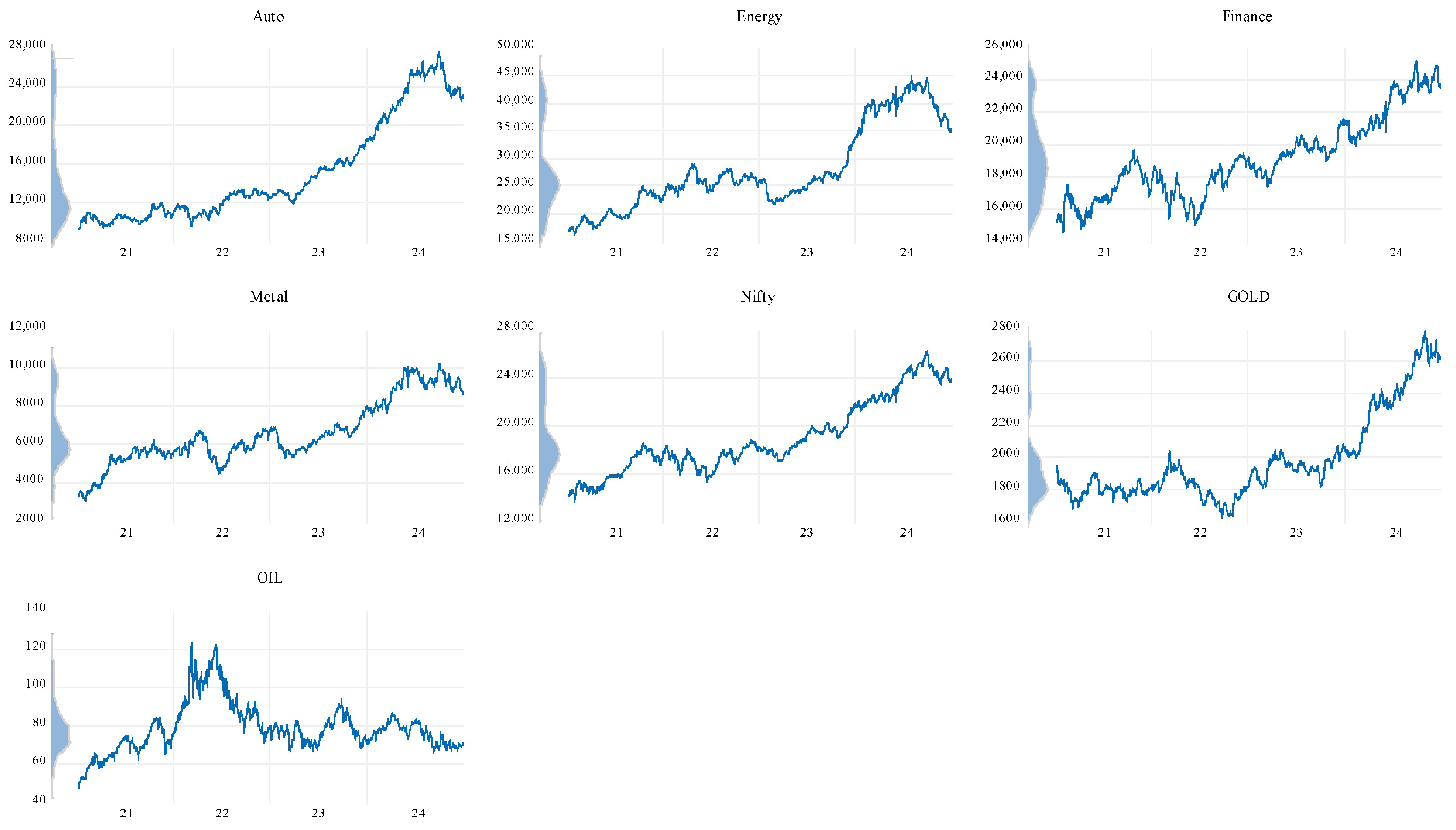
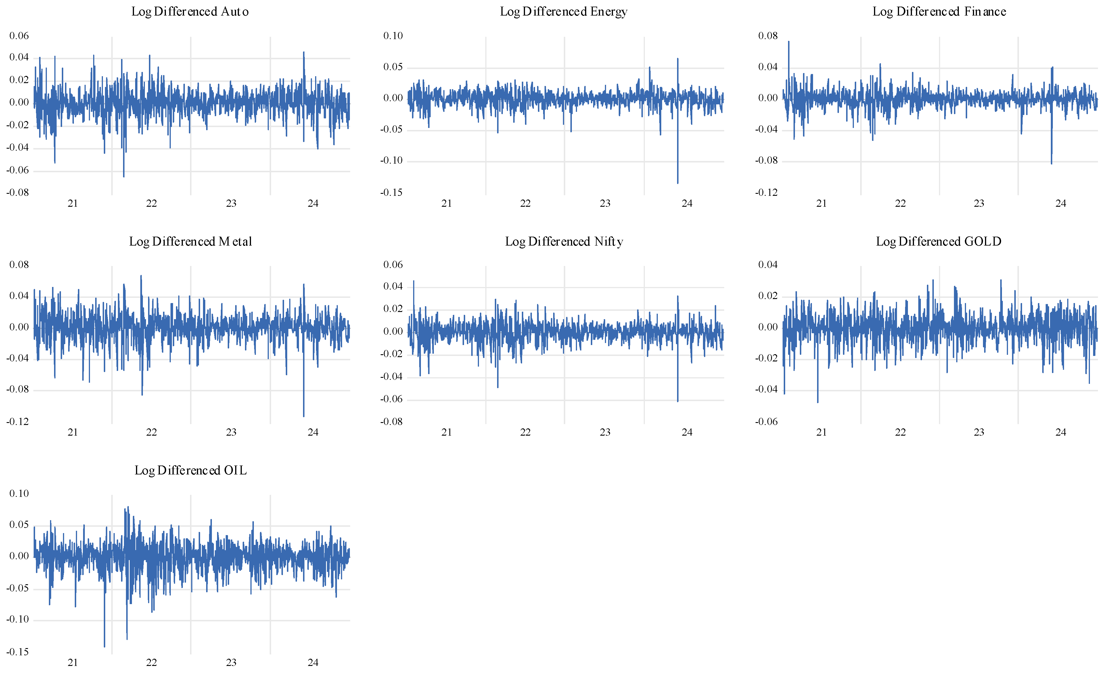
4.1. Descriptive Statistics
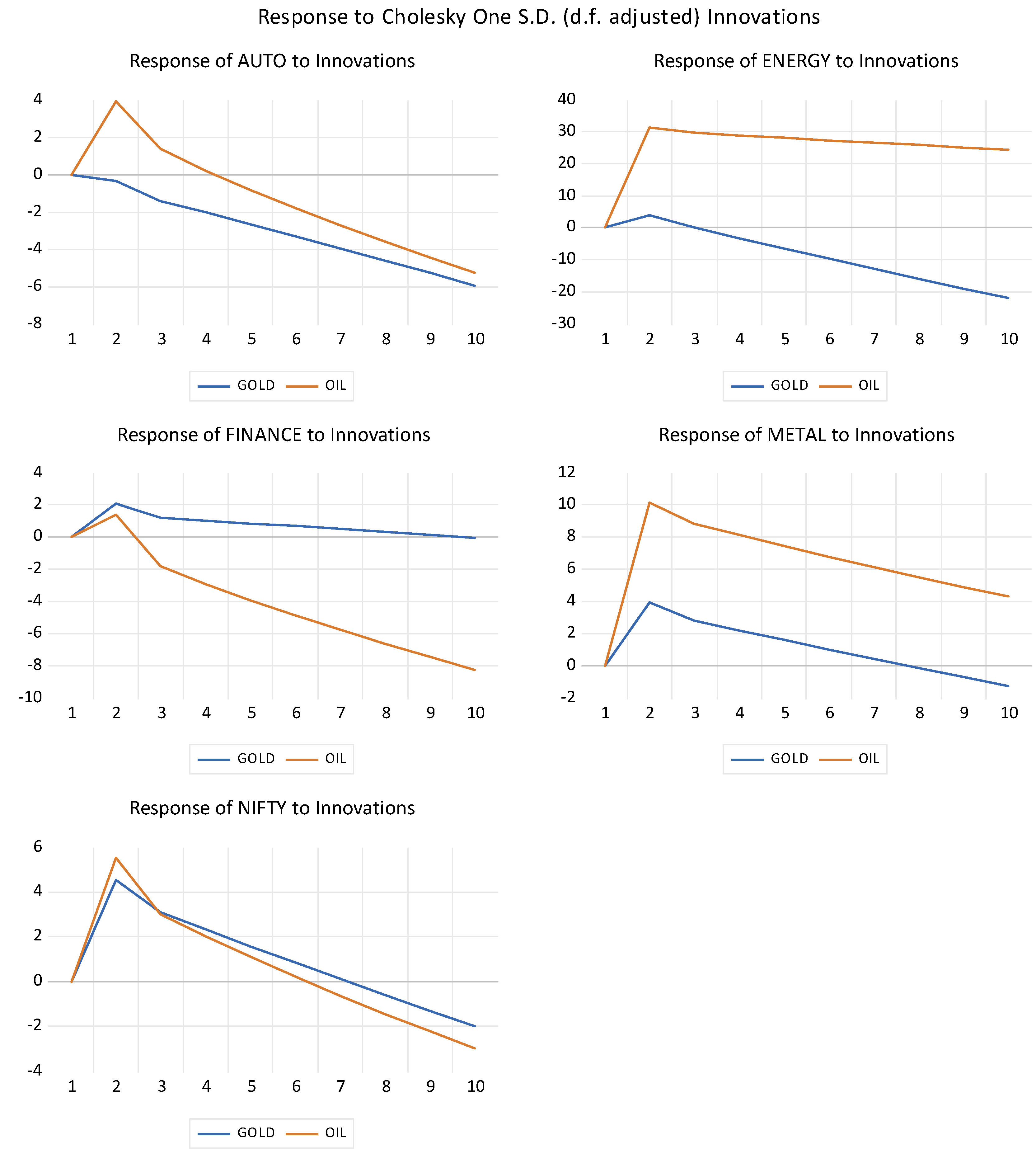
Figure 1 and Figure 2 depict the price trends and log differentiated returns of different indices from January 2021 to December 2024. The auto, energy, finance, metal, and Nifty indices show consistent upward trends, indicating growth in these sectors during the post-COVID-19 recovery phase, likely driven by increased economic activity and investor confidence. In contrast, the gold index exhibits a general upward movement, though less pronounced, reflecting its role as a safe-haven asset. However, the oil index demonstrates significant volatility with no clear upward trend, highlighting fluctuations in global oil prices and demand–supply dynamics.
Table 1 presents the demographic information of the commodity and sectoral variables used in the study. The mean values suggest that energy has the highest average return at 17.579, followed by auto at 13.090. In contrast, gold has the lowest at 0.638. The standard deviations reveal varying levels of risk, with energy exhibiting the highest volatility (387.833) and gold the lowest (18.338). Skewness values indicate that most of the series are negatively skewed. Energy (−2.614) shows the strongest negative skew, indicating a tendency towards more significant negative returns. Kurtosis values are high, particularly for energy (41.939), suggesting fat tails or extreme outliers in the distribution. Jarque–Bera test results, marked with asterisks, confirm that all variables deviate significantly from normality. The Augmented Dickey–Fuller (ADF) and Kwiatkowski–Phillips–Schmidt–Shin (KPSS) test shows non-stationarity at level and stationarity at the first difference for all the indices. The ARCH-LM test that hypothesizes about the absence of ARCH effects has been rejected for all the indices at leg five (since we have used daily stock data), indicating the presence of heteroskedasticity and allowing for GARCH modeling.

4.2. The VAR Model

The Bayesian VAR, which is a better model than the standard VAR for small datasets and computational efficiency [52,53], is estimated and presented in Table 2. It shows the interdependence among sectoral spot indices along with gold and oil futures, with key insights derived from the coefficients, standard errors, and t-statistics (significance is indicated using an asterisk sign). The lagged values of the auto (−1) sector exhibit a strong positive relationship with its own future values, as indicated by the significant coefficient (1.0445, t = 34.164). However, its influence on other sectors is mostly insignificant. Energy, on the other hand, significantly influences multiple sectors. The first lag of energy has a strong positive effect on itself (0.8658, t = 27.093) and a significant negative impact on finance (−0.0632, t = −3.703), metal (−0.0326, t = −3.563), and Nifty (−0.0581, t = −4.292). Interestingly, the second lag of energy exhibits a positive influence on all these sectors, suggesting a delayed stabilizing effect. Similarly, finance (−1) and metal (−1) show strong autocorrelation, with coefficients of 0.9727 and 0.9906, respectively, implying that past values are strong predictors of their own future values. However, their cross-sector influences remain insignificant. On the other hand, the impact of commodity prices, particularly oil (−1), shows a significant positive impact on energy (15.970, t = 3.180) and metal (5.1705, t = 3.584), but this effect reverses and becomes negative at lag 2, indicating a short-term boosting effect followed by a correction. Gold (−1) prices primarily exhibit strong autocorrelation, with a coefficient of 0.9430, indicating its self-persistence. Similarly, Nifty, representing the broader stock market, is significantly influenced by its own past values (1.0460). Thus, it can be inferred from the above that commodity prices, especially oil, show a short-lived positive impact on energy and metal before stabilizing, while gold remains largely self-driven.
The impulse response function (IRF) graphs given in Figure 3 show the impact of one standard deviation shock in gold and oil prices on different sectors—auto, energy, finance, metal, and Nifty—over a 10-period horizon. In most cases, oil price shocks exhibit a stronger and more immediate impact compared with the shock from gold prices. The energy sector responds most significantly to oil shocks, with a sharp initial increase followed by a gradual decline, while gold shocks have a weaker but negative effect. Similarly, the auto and metal sectors show a noticeable initial positive response to oil shocks, followed by a declining trend, whereas gold shocks elicit a more muted reaction. The finance sector reacts negatively to both shocks initially but stabilizes over time, with oil shocks showing a larger downward impact. Lastly, the Nifty index follows a similar pattern to auto and metal, with an initial spike due to oil shocks and then a gradual decrease.

4.3. The Diebold–Yilmaz Spillover Index

The Diebold–Yilmaz Spillover Connectedness Index plots presented in Figure 4 highlight the dynamic but relatively limited hedging abilities of gold and oil with Indian sectoral indices. For gold, the spillover effects with sectors such as auto, finance, and Nifty are moderate, showing occasional spikes during periods of market volatility. However, the overall trends suggest that gold’s traditional role as a safe-haven asset is not strongly evident in this period, likely due to evolving market conditions and diminished investor reliance on gold as a risk mitigation tool. The relatively stable and low spillovers with sectors like energy and metal further indicate that gold’s hedging effectiveness is weak and fails to provide consistent protection against sectoral risks.
Oil, on the other hand, shows more pronounced spillovers with the energy, metal, and auto sectors, reflecting its fundamental connection to these industries. However, the variability in spillover intensity across time suggests that oil’s ability to hedge against sectoral risks is context-dependent, with sharp spikes primarily driven by global supply-chain disruptions or geopolitical tensions. These fluctuations underline oil’s limited and inconsistent role as a hedging instrument during the post-COVID-19 recovery period. The analysis demonstrates that neither gold nor oil provides better hedging capabilities for Indian sectoral indices in the studied timeframe, emphasizing the need for diversified strategies to mitigate risks in the post-pandemic economic environment.

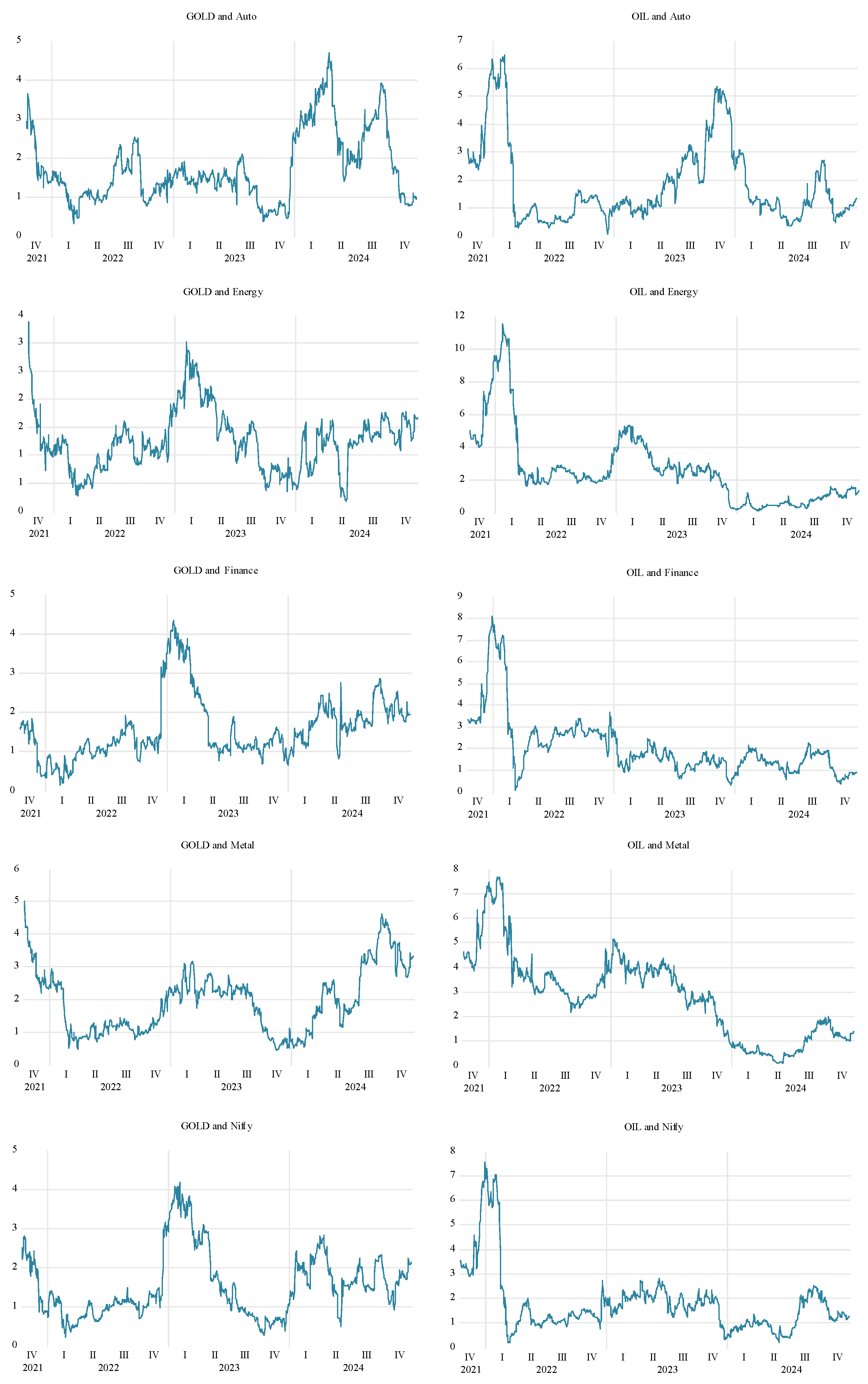
4.4. ADCC-GARCH Model

The ADCC-GARCH model results presented in Table 3 reveal valuable insights into the volatility dynamics and asymmetries across the indices analyzed. Starting with the mean return (μ), most indices exhibit statistically significant values, albeit small, highlighting modest average returns over the analyzed period. For instance, the Nifty (μ = 0.0008, p = 0.002) and metal (μ = 0.0011, p = 0.021) indices show notable returns, reflecting strong market performance. In contrast, gold and oil show insignificant mean returns, indicating lower average returns or potential price stability. The AR1 and MA1 coefficients are significant for energy and metal, suggesting a stronger short-term dependence in returns and market adjustments in these indices, while others, like Nifty and finance, show weaker autocorrelations.
The conditional variance parameters (ω, α1, β1) further highlight crucial volatility dynamics. The persistence of volatility (β1) is exceptionally high for gold (β1 = 0.9957), signaling those shocks to gold’s volatility decay slowly, consistent with its traditional role as a safe haven. Similarly, high persistence is observed for oil (β1 = 0.8701) and finance (β1 = 0.8488), indicating prolonged volatility effects. The significant DCC parameters (DCC-α1 = 0.0195, DCC-β1 = 0.8876) confirm dynamic conditional correlations among the indices, suggesting that volatility transmission and time-varying co-movements are prevalent across the assets. Energy’s notable α1 = 0.2222 suggests it reacts more quickly to new market information, making it sensitive to shocks. This is contrasted by gold, with a minimal α1 = 0.002, which implies minimal responsiveness to market shocks, aligning with its low-risk nature.
The asymmetric effect, represented by the parameter ω, provides insights into how shocks of different signs impact the volatility of the indices. Across the results, ω is statistically significant for energy (p = 0.009), Finance (p = 0.011), gold (p = 0.009), and oil (p = 0.005), indicating the presence of asymmetry in these markets. This implies that negative shocks (bad news) tend to affect volatility differently than positive shocks (good news), a characteristic often linked to investor sentiment and market risk aversion. For example, gold and oil, as commodities, exhibit significant asymmetric effects due to their sensitivity to geopolitical events and macroeconomic uncertainties, which can amplify volatility during adverse market conditions. Conversely, indices like auto and Nifty show insignificant ω values, suggesting relatively symmetric responses to shocks, which could reflect more stable investor behavior and reduced sensitivity to market news. These observations highlight the diverse nature of volatility responses across asset classes, driven by their underlying economic and market characteristics.
The analysis reveals that the asymmetric effects, as represented by the parameter ω, are significant for certain asset classes like gold, oil, and energy, indicating that negative shocks (e.g., adverse news or market downturns) have a more pronounced impact on volatility compared with positive shocks. This asymmetry aligns with the leverage effect observed in financial markets, where bad news tends to increase perceived risk and uncertainty, leading to heightened volatility [54,55]. Commodities such as gold and oil, being highly sensitive to geopolitical and macroeconomic factors, exhibit strong asymmetric volatility responses due to their role as hedging instruments and their dependency on external factors like supply disruptions or inflationary pressures. On the other hand, sectoral indices like auto and Nifty exhibit relatively symmetric behavior, suggesting that these markets may experience more stable investor sentiment or are better diversified against external shocks. These findings underscore the heterogeneous nature of volatility dynamics across asset classes, emphasizing the importance of considering asymmetry when modeling risk and making portfolio decisions.

4.5. Dynamic Hedge Ratio and Hedging Effectiveness

Table 4 presents the average dynamic hedge ratios and hedging effectiveness for various asset pairs, reflecting the ability of one asset to hedge the risk of another. Notably, Nifty exhibits high average hedge ratios (more than one for Nifty–metal, Nifty–finance, and Nifty–energy) and strong hedging effectiveness (0.68 to 0.87), indicating its suitability as a robust hedging instrument against these indices. In contrast, gold shows relatively low hedge ratios and modest effectiveness, with gold–metal (0.18) and gold–finance (0.12) performing better compared with other pairs involving gold. Oil, across all its combinations, has minimal hedge ratios (all below 0.1) and poor effectiveness, suggesting limited potential as a hedge. Pairs like metal–finance and metal–energy demonstrate moderate hedge ratios (0.34 and 0.47) and effectiveness (0.76 and 0.62), indicating better hedging performance. Overall, indices like Nifty and metal appear to be more effective for risk management, while oil and gold are less efficient as hedging instruments.
The findings suggest that both gold and oil exhibit limited effectiveness as hedging instruments against Indian sectoral indices, with consistently low average hedge ratios and hedging effectiveness. The relatively higher hedging effectiveness of gold with metal (0.18) and finance (0.12) compared with other pairs indicates some potential to mitigate sector-specific risks, likely due to its status as a traditional safe-haven asset during periods of economic uncertainty [56]. However, its overall weak performance across most indices highlights its limited applicability in the dynamic Indian market. Conversely, oil demonstrates uniformly poor hedging effectiveness and minimal hedge ratios, reflecting its inability to offset sectoral risks effectively. This contradicts prior studies indicating that commodities like gold and oil could be used as better hedging funds than sectoral indices [57]. On the other hand, crude oil prices often exhibit greater volatility and weaker correlations with equity markets, reducing their hedging potential [58]. This observation provides an interesting aspect of the commodities markets being poor in hedging ability even though they exhibit poor correlation with the sectoral indices [15]. These results underscore the need to explore alternative commodities or financial instruments to enhance risk mitigation strategies in sectoral portfolios.

5. Conclusions

The analysis of spillover dynamics between gold, oil, and Indian sectoral indices during the post-COVID-19 recovery period underscores the necessity for innovative risk management strategies, as both commodities exhibit limited and inconsistent hedging efficacy. The poor, stable spillover effect of gold in most sectors challenges its traditional role as a safe-haven asset. Oil, on the other hand, exhibits relatively higher but volatile spillover effects, particularly with sectors closely tied to energy and industrial activities, reflecting its dependence on external economic and geopolitical factors. For investors and portfolio managers, these findings advocate a shift toward dynamic, diversified strategies that integrate alternative assets or adaptive hedging mechanisms to counter sector-specific vulnerabilities intensified by geopolitical and economic uncertainties reflected in the post-COVID-19 period. Policymakers, conversely, can leverage these insights to strengthen financial resilience by strategically addressing sectoral interdependencies and systemic risks. Both gold and oil have proved to be ineffective hedging tools for sectoral risks in the Indian market during the post-COVID-19 period, highlighting a nuanced observation and warranting alternative hedging mechanisms or diversified approaches to risk management.

6. Limitations and Scope

This research has several limitations that should be acknowledged. Firstly, this study focuses solely on the post-COVID-19 period (January 2021 to December 2024), which may not capture long-term trends or structural shifts in the market. Secondly, it examines only two commodities, gold and oil, as hedging tools, potentially overlooking other assets or instruments that may offer better hedging potential. Additionally, the analysis is restricted to select sectoral indices, which may not fully represent the diversity of the Indian market. The methodology, while robust, relies on specific model assumptions, such as the Diebold–Yilmaz spillover index, which may not account for all complexities of financial spillovers. Lastly, external factors such as regulatory changes, geopolitical events, and macroeconomic shocks, which can significantly influence market dynamics, are not explicitly incorporated into the analysis. Another limitation of this study lies in the insignificance of certain findings in the VAR and ADCC-GARCH models, which may be due to structural shifts in the post-COVID-19 period. Future research could refine these models by incorporating higher-frequency data or alternative econometric approaches like quantile regression models to better capture the spillover effects and explore some novel observations.
Future studies could expand the scope by exploring additional commodities, such as silver or cryptocurrency, to assess their hedging potential against sectoral indices. Additionally, investigating the impact of external factors, such as geopolitical risks, interest rate changes, or policy interventions, would enhance the contextual understanding of market interactions. As such, comparative analysis across multiple emerging markets could also offer valuable insights into regional variations in hedging and connectedness.

Author Contributions

Conceptualization, N.M. and A.K.P.; methodology, software, N.M.; validation, N.M. and S.K.C.; formal analysis, N.M.; investigation, A.K.P.; resources, data curation, S.K.C.; writing—original draft preparation, writing—review and editing, N.M.; visualization, S.K.C.; supervision, A.K.P.; project administration, N.M. All authors have read and agreed to the published version of the manuscript.

Funding

This research received no external funding.

Institutional Review Board Statement

Not applicable.

Informed Consent Statement

Not applicable.

Data Availability Statement

Data will be provided on request.

Conflicts of Interest

The authors declare no conflicts of interest.

References

  1. Hamilton, J.D.; Wu, J.C. Effects of Index-Fund Investing on Commodity Futures Prices. Int. Econ. Rev. 2015, 56, 187–205. [Google Scholar] [CrossRef]
  2. Just, M.; Luczak, A. Assessment of Conditional Dependence Structures in Commodity Futures Markets Using Copula-GARCH Models and Fuzzy Clustering Methods. Sustainability 2020, 12, 2571. [Google Scholar] [CrossRef]
  3. Tang, K.; Xiong, W. Index Investment and the Financialization of Commodities. Financ. Anal. J. 2012, 68, 54–74. [Google Scholar] [CrossRef]
  4. Irwin, S.H.; Sanders, D.R. Index Funds, Financialization, and Commodity Futures Markets. Appl. Econ. Perspect. Policy 2011, 33, 1–31. [Google Scholar] [CrossRef]
  5. Irwin, S.H.; Sanders, D.R. Financialization and Structural Change in Commodity Futures Markets. J. Agric. Appl. Econ. 2012, 44, 371–396. [Google Scholar] [CrossRef]
  6. Ederer, S.; Heumesser, C.; Staritz, C. Financialization and Commodity Prices—An Empirical Analysis for Coffee, Cotton, Wheat and Oil. Int. Rev. Appl. Econ. 2016, 30, 462–487. [Google Scholar] [CrossRef]
  7. Chordia, T.; Subrahmanyam, A.; Anshuman, V.R. Trading Activity and Expected Stock Returns. J. Financ. Econ. 2001, 59, 3–32. [Google Scholar] [CrossRef]
  8. Datar, V.T.; Naik, N.Y.; Radcliffe, R. Liquidity and Stock Returns: An Alternative Test. J. Financ. Mark. 1998, 1, 203–219. [Google Scholar] [CrossRef]
  9. Liu, G.; Guo, X. Forecasting Stock Market Volatility Using Commodity Futures Volatility Information. Resour. Policy 2022, 75, 102481. [Google Scholar] [CrossRef]
  10. Rzayev, K.; Ibikunle, G. A State-Space Modeling of the Information Content of Trading Volume. J. Financ. Mark. 2019, 46, 100507. [Google Scholar] [CrossRef]
  11. Diebold, F.X.; Yilmaz, K. Measuring Financial Asset Return and Volatility Spillovers, with Application to Global Equity Markets. Econ. J. 2009, 119, 158–171. [Google Scholar] [CrossRef]
  12. Diebold, F.X.; Yilmaz, K. On the Past, Present, and Future of the Diebold–Yilmaz Approach to Dynamic Network Connectedness. J. Econom. 2023, 234, 115–120. [Google Scholar] [CrossRef]
  13. Basher, S.A.; Sadorsky, P. Hedging Emerging Market Stock Prices with Oil, Gold, VIX, and Bonds: A Comparison between DCC, ADCC and GO-GARCH. Energy Econ. 2016, 54, 235–247. [Google Scholar] [CrossRef]
  14. Yadav, N.; Singh, A.B.; Tandon, P. Volatility Spillover Effects between Indian Stock Market and Global Stock Markets: A DCC-GARCH Model. FIIB Bus. Rev. 2023. [Google Scholar] [CrossRef]
  15. Maharana, N.; Panigrahi, A.K.; Chaudhury, S.K.; Uprety, M.; Barik, P.; Kulkarni, P. Economic Resilience in Post-Pandemic India: Analysing Stock Volatility and Global Links Using VAR-DCC-GARCH and Wavelet Approach. J. Risk Financ. Manag. 2025, 18, 18. [Google Scholar]
  16. Singhal, S.; Ghosh, S. Returns and Volatility Linkages between International Crude Oil Price, Metal and Other Stock Indices in India: Evidence from VAR-DCC-GARCH Models. Resour. Policy 2016, 50, 276–288. [Google Scholar] [CrossRef]
  17. Ozkan, O.; Abosedra, S.; Sharif, A.; Alola, A.A. Dynamic Volatility among Fossil Energy, Clean Energy and Major Assets: Evidence from the Novel DCC-GARCH. Econ. Chang. Restruct. 2024, 57, 98. [Google Scholar] [CrossRef]
  18. Armah, M.; Amewu, G.; Bossman, A. Time-Frequency Analysis of Financial Stress and Global Commodities Prices: Insights from Wavelet-Based Approaches. Cogent Econ. Financ. 2022, 10, 2114161. [Google Scholar] [CrossRef]
  19. Torrence, C.; Compo, G.P. A Practical Guide to Wavelet Analysis. Bull. Am. Meteorol. Soc. 1998, 79, 61–78. [Google Scholar] [CrossRef]
  20. Grinsted, A.; Moore, J.C.; Jevrejeva, S. Application of the Cross Wavelet Transform and Wavelet Coherence to Geophysical Time Series. Nonlinear Process. Geophys. 2004, 11, 561–566. [Google Scholar] [CrossRef]
  21. Wang, J. Application of Wavelet Transform Image Processing Technology in Financial Stock Analysis. J. Intell. Fuzzy Syst. 2021, 40, 2017–2027. [Google Scholar] [CrossRef]
  22. Khalfaoui, R.; Boutahar, M.; Boubaker, H. Analyzing Volatility Spillovers and Hedging between Oil and Stock Markets: Evidence from Wavelet Analysis. Energy Econ. 2015, 49, 540–549. [Google Scholar] [CrossRef]
  23. Ersin, Ö.Ö.; Bildirici, M. Financial Volatility Modeling with the GARCH-MIDAS-LSTM Approach: The Effects of Economic Expectations, Geopolitical Risks and Industrial Production during COVID-19. Mathematics 2023, 11, 1785. [Google Scholar] [CrossRef]
  24. Aliyev, F.; Ajayi, R.; Gasim, N. Modelling Asymmetric Market Volatility with Univariate GARCH Models: Evidence from Nasdaq-100. J. Econ. Asymmetries 2020, 22, e00167. [Google Scholar] [CrossRef]
  25. Shahzad, S.J.H.; Naeem, M.A.; Peng, Z.; Bouri, E. Asymmetric Volatility Spillover among Chinese Sectors during COVID-19. Int. Rev. Financ. Anal. 2021, 75, 101754. [Google Scholar] [CrossRef]
  26. Chkili, W. Dynamic Correlations and Hedging Effectiveness between Gold and Stock Markets: Evidence for BRICS Countries. Res. Int. Bus. Financ. 2016, 38, 22–34. [Google Scholar] [CrossRef]
  27. Chkili, W.; Aloui, C.; Nguyen, D.K. Instabilities in the Relationships and Hedging Strategies between Crude Oil and US Stock Markets: Do Long Memory and Asymmetry Matter? J. Int. Financ. Mark. Inst. Money 2014, 33, 354–366. [Google Scholar] [CrossRef]
  28. Sadorsky, P. Modeling Volatility and Conditional Correlations between Socially Responsible Investments, Gold and Oil. Econ. Model. 2014, 38, 609–618. [Google Scholar] [CrossRef]
  29. Arouri, M.E.H.; Jouini, J.; Nguyen, D.K. On the Impacts of Oil Price Fluctuations on European Equity Markets: Volatility Spillover and Hedging Effectiveness. Energy Econ. 2012, 34, 611–617. [Google Scholar] [CrossRef]
  30. Coudert, V.; Raymond-Feingold, H. Gold and Financial Assets: Are There Any Safe Havens in Bear Markets? Econ. Bull. 2011, 31, 1613–1622. [Google Scholar]
  31. Baur, D.G.; Lucey, B.M. Is Gold a Hedge or a Safe Haven? An Analysis of Stocks, Bonds and Gold. Financ. Rev. 2010, 45, 217–229. [Google Scholar] [CrossRef]
  32. Abdelhedi, M.; Boujelbène-Abbes, M. Transmission of Shocks between Chinese Financial Market and Oil Market. Int. J. Emerg. Mark. 2020, 15, 262–286. [Google Scholar] [CrossRef]
  33. Vardar, G.; Coşkun, Y.; Yelkenci, T. Shock Transmission and Volatility Spillover in Stock and Commodity Markets: Evidence from Advanced and Emerging Markets. Eurasian Econ. Rev. 2018, 8, 231–288. [Google Scholar] [CrossRef]
  34. Creti, A.; Joëts, M.; Mignon, V. On the Links between Stock and Commodity Markets’ Volatility. Energy Econ. 2013, 37, 16–28. [Google Scholar] [CrossRef]
  35. Marfatia, H.A.; Ji, Q.; Luo, J. Forecasting the Volatility of Agricultural Commodity Futures: The Role of Co-Volatility and Oil Volatility. J. Forecast. 2022, 41, 383–404. [Google Scholar] [CrossRef]
  36. Quintino, D.; Ogino, C.; Haq, I.U.; Ferreira, P.; Oliveira, M. An Analysis of Dynamic Correlations among Oil, Natural Gas and Ethanol Markets: New Evidence from the Pre- and Post-COVID-19 Crisis. Energies 2023, 16, 2349. [Google Scholar] [CrossRef]
  37. Fang, Y.; Shao, Z. The Russia-Ukraine Conflict and Volatility Risk of Commodity Markets. Financ. Res. Lett. 2022, 50, 103264. [Google Scholar] [CrossRef]
  38. Bouri, E.; Lucey, B.; Saeed, T.; Vo, X.V. The Realized Volatility of Commodity Futures: Interconnectedness and Determinants. Int. Rev. Econ. Financ. 2021, 73, 139–151. [Google Scholar] [CrossRef]
  39. Ding, S.; Cui, T.; Zheng, D.; Du, M. The Effects of Commodity Financialization on Commodity Market Volatility. Resour. Policy 2021, 73, 102220. [Google Scholar] [CrossRef]
  40. Salisu, A.A.; Vo, X.V.; Lawal, A. Hedging Oil Price Risk with Gold during COVID-19 Pandemic. Resour. Policy 2021, 70, 101897. [Google Scholar] [CrossRef]
  41. Akhtaruzzaman, M.; Boubaker, S.; Lucey, B.M.; Sensoy, A. Is Gold a Hedge or a Safe-Haven Asset in the COVID–19 Crisis? Econ. Model. 2021, 102, 105588. [Google Scholar] [CrossRef]
  42. Tarchella, S.; Khalfaoui, R.; Hammoudeh, S. The Safe Haven, Hedging, and Diversification Properties of Oil, Gold, and Cryptocurrency for the G7 Equity Markets: Evidence from the Pre- and Post-COVID-19 Periods. Res. Int. Bus. Financ. 2024, 67, 102125. [Google Scholar] [CrossRef]
  43. Ntare, H.B.; Mwamba, J.W.M.; Adekambi, F. Dynamic Correlation and Hedging Ability of Precious Metals in Pre- and Post-COVID Periods. Cogent Econ. Financ. 2024, 12, 2382375. [Google Scholar] [CrossRef]
  44. Arfaoui, N.; Yousaf, I.; Jareño, F. Return and Volatility Connectedness between Gold and Energy Markets: Evidence from the Pre- and Post-COVID Vaccination Phases. Econ. Anal. Policy 2023, 77, 617–634. [Google Scholar] [CrossRef]
  45. Penone, C.; Giampietri, E.; Trestini, S. Hedging Effectiveness of Commodity Futures Contracts to Minimize Price Risk: Empirical Evidence from the Italian Field Crop Sector. Risks 2021, 9, 213. [Google Scholar] [CrossRef]
  46. Huang, H.; Xiong, T. A Good Hedge or Safe Haven? The Hedging Ability of China’s Commodity Futures Market under Extreme Market Conditions. J. Futures Mark. 2023, 43, 968–1035. [Google Scholar] [CrossRef]
  47. Ciner, C.; Gurdgiev, C.; Lucey, B.M. Hedges and Safe Havens: An Examination of Stocks, Bonds, Gold, Oil and Exchange Rates. Int. Rev. Financ. Anal. 2013, 29, 202–211. [Google Scholar] [CrossRef]
  48. Maharana, N.; Panigrahi, A.K.; Chaudhury, S.K. Volatility Persistence and Spillover Effects of Indian Market in the Global Economy: A Pre- and Post-Pandemic Analysis Using VAR-BEKK-GARCH Model. J. Risk Financ. Manag. 2024, 17, 294. [Google Scholar] [CrossRef]
  49. Bouri, E.; Jain, A.; Biswal, P.C.; Roubaud, D. Cointegration and Nonlinear Causality amongst Gold, Oil, and the Indian Stock Market: Evidence from Implied Volatility Indices. Resour. Policy 2017, 52, 201–206. [Google Scholar] [CrossRef]
  50. Jose, A.; Jose, N. Exploring the Effectiveness of Hedging in the Indian Commodity Market: A Comparative Analysis of Constant and Dynamic Hedge Ratios Across Agricultural and Non-Agricultural Commodities. Int. J. Multidiscip. Res. 2024, 6, 1–15. [Google Scholar] [CrossRef]
  51. Gupta, S.; Choudhary, H.; Agarwal, D.R. Hedging Efficiency of Indian Commodity Futures. Paradigm 2017, 21, 1–20. [Google Scholar] [CrossRef]
  52. Israel, T.O.M.; Kingdom, N.; Yvonne, D.A.; Ike, W.A. Application of Bayesian Vector Autoregressive Models in the Analysis of Quasi Money and Money Supply: A Case Study of Nigeria. Asian J. Probab. Stat. 2023, 25, 108–117. [Google Scholar] [CrossRef]
  53. Ribeiro Ramos, F.F. Forecasts of Market Shares from VAR and BVAR Models: A Comparison of Their Accuracy. Int. J. Forecast. 2003, 19, 95–110. [Google Scholar] [CrossRef]
  54. Black, F. The Pricing of Commodity Contracts. J. Financ. Econ. 1976, 3, 167–179. [Google Scholar] [CrossRef]
  55. Engle, R.F.; Ng, V.K. Measuring and Testing the Impact of News on Volatility. J. Financ. 1993, 48, 1749–1778. [Google Scholar] [CrossRef]
  56. Baur, D.G.; McDermott, T.K. Is Gold a Safe Haven? International Evidence. J. Bank. Financ. 2010, 34, 1886–1898. [Google Scholar]
  57. Pandey, V. Does Commodity Exposure Benefit Traditional Portfolios? Evidence from India. Invest. Manag. Financ. Innov. 2023, 20, 36–49. [Google Scholar] [CrossRef]
  58. Filis, G.; Degiannakis, S.; Floros, C. Dynamic Correlation between Stock Market and Oil Prices: The Case of Oil-Importing and Oil-Exporting Countries. Int. Rev. Financ. Anal. 2011, 20, 152–164. [Google Scholar] [CrossRef]
Figure 1. Trend of the selected commodity futures and sectoral indices.
Commodities 04 00005 g001
Figure 2. Daily log differentiated return plot of the selected sectors and commodity futures.
Commodities 04 00005 g002
Figure 3. IRF curves for response of sectoral indices to the innovations of gold and oil.
Commodities 04 00005 g003
Figure 4. Diebold–Yilmaz spillover index plot (200-day windows, 10-step horizon).
Commodities 04 00005 g004
Table 1. Descriptive statistics of the selected indices.
AutoEnergyFinanceMetalNiftyGoldOil
Mean13.09017.5798.0395.2049.2920.6380.023
Median6.60017.3252.6256.0005.2750.5500.090
Maximum1090.4502726.4001109.150516.450735.85058.1008.010
Minimum−1007.950−5357.800−1776.900−1068.400−1379.400−93.100−15.000
Std. Dev.182.715387.833207.506111.602164.76718.3381.969
Skewness−0.392−2.614−0.646−1.133−0.710−0.602−0.814
Kurtosis7.39141.93910.57012.6529.6035.3158.942
Jarque–Bera858.918 *66,629.855 *2546.040 *4243.143 *1968.809 *293.884 *1638.216 *
ADF (Level)−1.903−1.330−3.128−2.474−2.298−1.370−2.359
ADF(1-Diff.)−7.416 *−35.511 *−11.029 *−33.503 *−32.672 *−8.743 *−10.380 *
KPSS (Level)0.822 *0.493 *0.514 *0.486 *0.654 *0.780 *0.505 *
KPSS (1-Diff.)0.1080.1280.0240.0650.0520.0270.060
ARCH-LM (Leg-5)8.450 *3.784 *2.221 **3.762 *2.661 **2.676 **23.037 *
Note: ** significant at 5%; * significant at 1%.
Table 2. VAR Model presented for oil and all indices.
AutoEnergyFinanceMetalNiftyOilGold
Auto (−1)Coeff.1.04450.06700.04370.01310.03660.00000.0013
S.E.0.03060.06380.03420.01830.02720.00030.0031
t34.1649 *1.05041.27600.71551.34830.03520.4212
Auto (−2)Coeff.−0.0419−0.0499−0.0261−0.0075−0.0228−0.0001−0.0008
S.E.0.03040.06350.03410.01830.02700.00030.0031
t−1.3751−0.7851−0.7661−0.4119−0.8435−0.4415−0.2476
Energy (−1)Coeff.−0.04860.8658−0.0632−0.0326−0.0581−0.0002−0.0004
S.E.0.01520.03200.01710.00910.01350.00020.0015
t−3.2049 *27.0930 *−3.7031 *−3.5632 *−4.2924 *−0.9456−0.2366
Energy (−2)Coeff.0.04780.11130.04900.03130.04940.0002−0.0001
S.E.0.01490.03140.01680.00900.01330.00020.0015
t3.2030 *3.5426 *2.9201 *3.4852 *3.7148 *1.2066−0.0405
Finance (−1)Coeff.−0.0017−0.03270.97270.0033−0.00280.0000−0.0019
S.E.0.03090.06490.03500.01860.02760.00030.0031
t−0.0540−0.504327.8257 *0.1754−0.1015−0.0971−0.6217
Finance (−2)Coeff.−0.0302−0.0521−0.0469−0.0117−0.0352−0.0002−0.0010
S.E.0.02890.06050.03260.01740.02580.00030.0029
t−1.0468−0.8605−1.4355−0.6723−1.3640−0.6358−0.3595
Metal (−1)Coeff.−0.04540.1619−0.08620.9906−0.03800.00040.0035
S.E.0.05130.10760.05770.03100.04580.00060.0052
t−0.88481.5045−1.492631.9130 *−0.83000.64650.6741
Metal (−2)Coeff.0.0388−0.17240.0928−0.00840.0453−0.0004−0.0022
S.E.0.05060.10610.05690.03060.04510.00050.0051
t0.7674−1.62471.6305−0.27391.0038−0.7200−0.4371
Nifty (−1)Coeff.0.04770.09630.08210.00581.04600.00010.0006
S.E.0.04310.09030.04850.02590.03860.00050.0043
t1.10831.06691.6940 ***0.224827.0910 *0.27040.1429
Nifty (−2)Coeff.−0.01840.0160−0.02180.0057−0.01970.00020.0029
S.E.0.04020.08420.04520.02420.03610.00040.0041
t−0.45870.1896−0.48230.2364−0.54510.42730.7158
Oil (−1)Coeff.1.979215.97090.70695.17052.79900.99670.1123
S.E.2.39535.02132.69471.44262.13630.02610.2419
t0.82633.1806 *0.26233.5841 *1.310238.2211 *0.4644
Oil (−2)Coeff.−2.4826−15.7458−1.1922−5.3217−3.1600−0.0229−0.1893
S.E.2.37314.97472.66971.42922.11640.02580.2397
t−1.0461−3.1652 *−0.4466−3.7235 *−1.4931−0.8867−0.7900
Gold (−1)Coeff.−0.01940.21980.11550.21470.2542−0.00110.9430
S.E.0.25700.53870.28910.15480.22920.00280.0260
t−0.07570.40790.39961.38741.1092−0.411636.2211 *
Gold (−2)Coeff.−0.0275−0.4329−0.1400−0.2518−0.30640.00110.0397
S.E.0.25480.53410.28660.15340.22720.00280.0258
t−0.1078−0.8105−0.4885−1.6407 ***−1.34830.40531.5376
CCoeff.227.4086363.8958458.595799.3629352.09161.800626.8175
S.E.127.8102267.9272143.788976.9754113.98541.386912.9067
t1.77931.35823.1894 *1.29083.0889 *1.29822.0778 **
Note: *** significant at 10%; ** significant at 5%; * significant at 1%.
Table 3. ADCC-GARCH Model.
IndicesParametersEstimateStd. Errort-ValueSig.
Autoμ0.00100.00042.39070.017
AR10.31460.35480.88670.375
MA1−0.25110.3460−0.72550.468
ω0.00000.00000.11750.906
α10.06570.19790.33190.740
β10.91870.23383.93010.000
Energyμ0.00100.00052.03340.042
AR10.90420.09529.49410.000
MA1−0.87380.1105−7.90740.000
ω0.00000.00002.62610.009
α10.22220.06663.33590.001
β10.47710.14693.24860.001
Financeμ0.00060.00031.76070.078
AR1−0.13560.1542−0.87920.379
MA10.19780.14451.36910.171
ω0.00000.00002.55240.011
α10.10880.02025.38510.000
β10.84880.031427.00560.000
Metalμ0.00110.00052.31310.021
AR1−0.87640.1186−7.38750.000
MA10.85570.12896.64020.000
ω0.00000.00001.25220.211
α10.15690.08741.79580.073
β10.69690.18483.77200.000
Niftyμ0.00080.00033.10820.002
AR1−0.14350.2159−0.66500.506
MA10.19620.20860.94070.347
ω0.00000.00001.12330.261
α10.13450.03174.23640.000
β10.82070.042219.44360.000
Goldμ0.00020.00030.86730.386
AR10.17380.17131.01490.310
MA1−0.22290.1686−1.32230.186
ω0.00000.00002.61430.009
α10.00200.000212.39440.000
β10.99570.00025546.04520.000
Oilμ0.00090.00061.36610.172
AR1−0.33450.2131−1.57000.116
MA10.37050.20731.78680.074
ω0.00000.00002.80250.005
α10.09470.01994.76050.000
β10.87010.021141.22700.000
JointDCC-α10.01950.00404.84840.000
JointDCC-β10.88760.023238.28110.000
Table 4. Dynamic Hedge Ratio and Hedging Effectiveness.
PairAverage Hedge RatioHedging Effectiveness
Oil–Nifty0.03190.79%
Oil–Metal0.09702.63%
Oil–Finance0.0338−0.49%
Oil–Energy0.03321.06%
Oil–Auto0.04650.20%
Gold–Nifty0.05717.65%
Gold–Metal0.231617.59%
Gold–Finance0.072411.96%
Gold–Energy0.07905.52%
Gold–Auto0.04973.34%
Nifty–Metal1.335687.12%
Nifty–Finance1.117671.67%
Nifty–Energy1.037775.36%
Nifty–Auto0.957467.90%
Metal–Finance0.342276.54%
Metal–Energy0.472262.40%
Metal–Auto0.369944.29%
Finance–Energy0.628840.37%
Finance–Auto0.600437.80%
Energy–Auto0.576366.16%
Disclaimer/Publisher’s Note: The statements, opinions and data contained in all publications are solely those of the individual author(s) and contributor(s) and not of MDPI and/or the editor(s). MDPI and/or the editor(s) disclaim responsibility for any injury to people or property resulting from any ideas, methods, instructions or products referred to in the content.

