Article

Tail Risk in Weather Derivatives

1
Risk Management Institute, National University of Singapore, Singapore 119244, Singapore
2
Department of Mathematics, National University of Singapore, Singapore 119077, Singapore
*
Author to whom correspondence should be addressed.
Commodities 2025, 4(2), 11; https://doi.org/10.3390/commodities4020011
Submission received: 16 April 2025 / Revised: 10 June 2025 / Accepted: 11 June 2025 / Published: 17 June 2025

Abstract

:
Weather derivative markets, particularly Chicago Mercantile Exchange (CME) Heating Degree Day (HDD) and Cooling Degree Day (CDD) futures, face challenges from complex temperature dynamics and spatially heterogeneous co-extremes that standard Gaussian models overlook. Using daily data from 13 major U.S. cities (2014–2024), we first construct a two-stage baseline model to extract standardized residuals isolating stochastic temperature deviations. We then estimate the Extreme Value Index (EVI) of HDD/CDD residuals, finding that the nonlinear degree-day transformation amplifies univariate tail risk, notably for warm-winter HDD events in northern cities. To assess multivariate extremes, we compute Tail Dependence Coefficient (TDC), revealing pronounced, geographically clustered tail dependence among HDD residuals and weaker dependence for CDD. Finally, we compare Gaussian, Student’s t, and Regular Vine Copula (R-Vine) copulas via joint VaR–ES backtesting. The R-Vine copula reproduces HDD portfolio tail risk, whereas elliptical copulas misestimate portfolio losses. These findings highlight the necessity of flexible dependence models, particularly R-Vine, to set margins, allocate capital, and hedge effectively in weather derivative markets.

1. Introduction

The increasing frequency and intensity of extreme weather events pose a substantial threat to global economic stability and growth [1,2]. Temperature extremes, hurricanes, floods, and prolonged droughts have disrupted key sectors, including agriculture, where yields collapse under anomalous heat or rainfall, and energy, where demand and production capacities fluctuate with temperature volatility [3,4,5]. Estimates suggest that up to 30 % of global GDP is directly exposed to weather variations, and under severe warming scenarios, projected economic damage may rise from approximately 11 % to 40 % of GDP [4,6]. These mounting vulnerabilities underscore the need for financial instruments to stabilize revenues and allocate capital in an increasingly erratic climate.
Weather derivatives are bespoke financial contracts whose payoffs depend on objectively measurable weather indices rather than indemnity claims [7]. By settling on deviation of indices from predetermined reference levels, they enable energy providers, agricultural firms, and other weather-exposed industries to hedge volumetric and revenue risks (for example, an electricity generator can offset reduced winter demand during a mild season) without proving actual losses [4,8]. The Chicago Mercantile Exchange (CME) Group, as the market leader, lists standardized futures and options on Heating Degree Day (HDD)/Cooling Degree Day (CDD) indices for major U.S. cities. Each HDD index accumulates daily average temperature shortfalls below 65   ° F ( 18.33   ° C ) , while each CDD index accumulates daily average temperature excesses above the same base. Payoffs are quoted in U.S. dollars per index point, ensuring transparency and comparability across regions. Initially traded over-the-counter beginning in 1997, with the first futures appearing in 1999, the weather derivatives market has expanded rapidly [9]. By 2025, it is projected to exceed $ 25 billion in volume, as extreme weather concerns intensify [3].
Pricing weather derivatives and managing their risks present distinct challenges. Because meteorological variables are non-tradable, weather markets remain incomplete, forcing practitioners to estimate a “market price" for risk rather than rely on perfectly hedgeable instruments [8,10]. Moreover, temperature series exhibit pronounced seasonality, autocorrelation, and conditional heteroskedasticity, violating the assumptions of standard option pricing frameworks such as Black-Scholes [4]. The very structure of HDD/CDD indices, where the “daily average” is derived from both daily maximum (block maxima) and minimum (block minima) temperatures, further amplifies heavy-tailed outcomes that Gaussian-based models tend to understate.
Existing approaches typically model temperature dynamics via Ornstein–Uhlenbeck processes [11,12,13], CARMA formulations [14,15,16,17], or seasonal Generalized Autoregressive Conditional Heteroskedasticity (GARCH)-type specifications [4,18,19], capturing mean reversion and volatility clustering but assuming Gaussian residuals. When multivariate dependence is addressed, often through simple Gaussian or Archimedean copulas, tail-risk and cross-location extremes remain inadequately captured. As a result, portfolio-level tail exposures in non-catastrophic but severe weather scenarios may be substantially misestimated. Furthermore, residual diagnostics from autoregressive models, which can reveal deviations from normality, are seldom exploited in this literature. Filling these gaps calls for a unified framework that integrates Extreme Value Theory (EVT) to quantify heavy-tailed behavior and employs more flexible multivariate copula constructions to model complex dependence structures. By doing so, one can better assess and hedge the often-overlooked tail risk inherent in HDD/CDD index portfolios [20,21,22,23,24].
Building on these observations, this study contributes by developing a unified empirical framework to quantify tail risks in CME-traded HDD/CDD futures from both univariate and multivariate perspectives. First, we employ a two-stage model to filter out trend, seasonality, and conditional heteroskedasticity, yielding standardized residuals that isolate the stochastic component of temperature variation. We then measure univariate tail thickness (via the Extreme Value Index (EVI)) of these residuals and use Tail Dependence Coefficient (TDC) to uncover geographically clustered co-extremes. Finally, we assess portfolio-level tail risk by comparing the out-of-sample performance of Gaussian, Student’s t, and Regular Vine Copula (R-Vine) copulas under a joint Value at Risk (VaR)–Expected Shortfall (ES) backtesting framework. By integrating baseline modeling, EVT-based tail estimation, and flexible copula constructions, this work provides both theoretical insights and practical guidance for weather-risk management.
The remainder of the paper is organized as follows. Section 2 describes the CME HDD/CDD contracts, introduces our two-stage baseline model for filtering temperature dynamics, and explains how we extract standardized residuals for EVT and dependence analysis. In Section 3, we quantify univariate tail risk by estimating the EVI for HDD/CDD residuals and discuss the implications for margin setting and hedging. Section 4 examines multivariate tail dependence via TDC, highlighting geographically clustered co-extremes and their impact on diversification. In Section 5, we assess portfolio-level tail risk by fitting Gaussian, Student’s t, and R-Vine copulas to the residuals and compare their out-of-sample VaR–ES performance through repeated cross-validation. Finally, Section 6 summarizes our findings, emphasizes the advantages of the flexible R-Vine approach for HDD risk management, and suggests for future research.

2. Background: Chicago Mercantile Exchange (CME) Temperature Derivatives and Baseline Modeling

2.1. Structure of CME Heating Degree Day (HDD)/ Cooling Degree Day (CDD) Index Futures

Heating Degree Day (HDD) and Cooling Degree Day (CDD) are cumulative indices that quantify deviations from a reference temperature, forming the basis for Chicago Mercantile Exchange (CME) degree-day index futures. For each day t,
T t = T t max + T t min 2
HDD t = max 0 , 65   ° F T t
CDD t = max 0 , T t 65   ° F
where the daily average T t is the arithmetic mean of the daily maximum (block maximum, T t max ) and daily minimum (block minimum, T t min ) temperatures recorded between 00:00 LST and 23:59 LST, capturing intra-day extremes [25].
CME HDD index accumulates daily HDD from November through March, and CME CDD index accumulates daily CDD from May through September. Corresponding contracts are quoted at $ 20 per index point in Fahrenheit for U.S. cities. Trading begins on the first day of the accrual period and ends on the last day, with settlement based on the published index.
Although CME lists weather futures for both domestic and international locations, we focus on 13 U.S. cities that together account for over 70 % of total HDD/CDD trading volume and have the longest continuous transactional history, providing robust, standardized settlement data [26]. These cities span diverse climates, including Mediterranean (Burbank, Sacramento), desert (Las Vegas), humid continental (Chicago, Minneapolis, Boston, New York, Philadelphia, Cincinnati), and humid subtropical (Houston, Atlanta), reflecting heterogeneous risk exposures and catering to hedging needs across the contiguous United States.

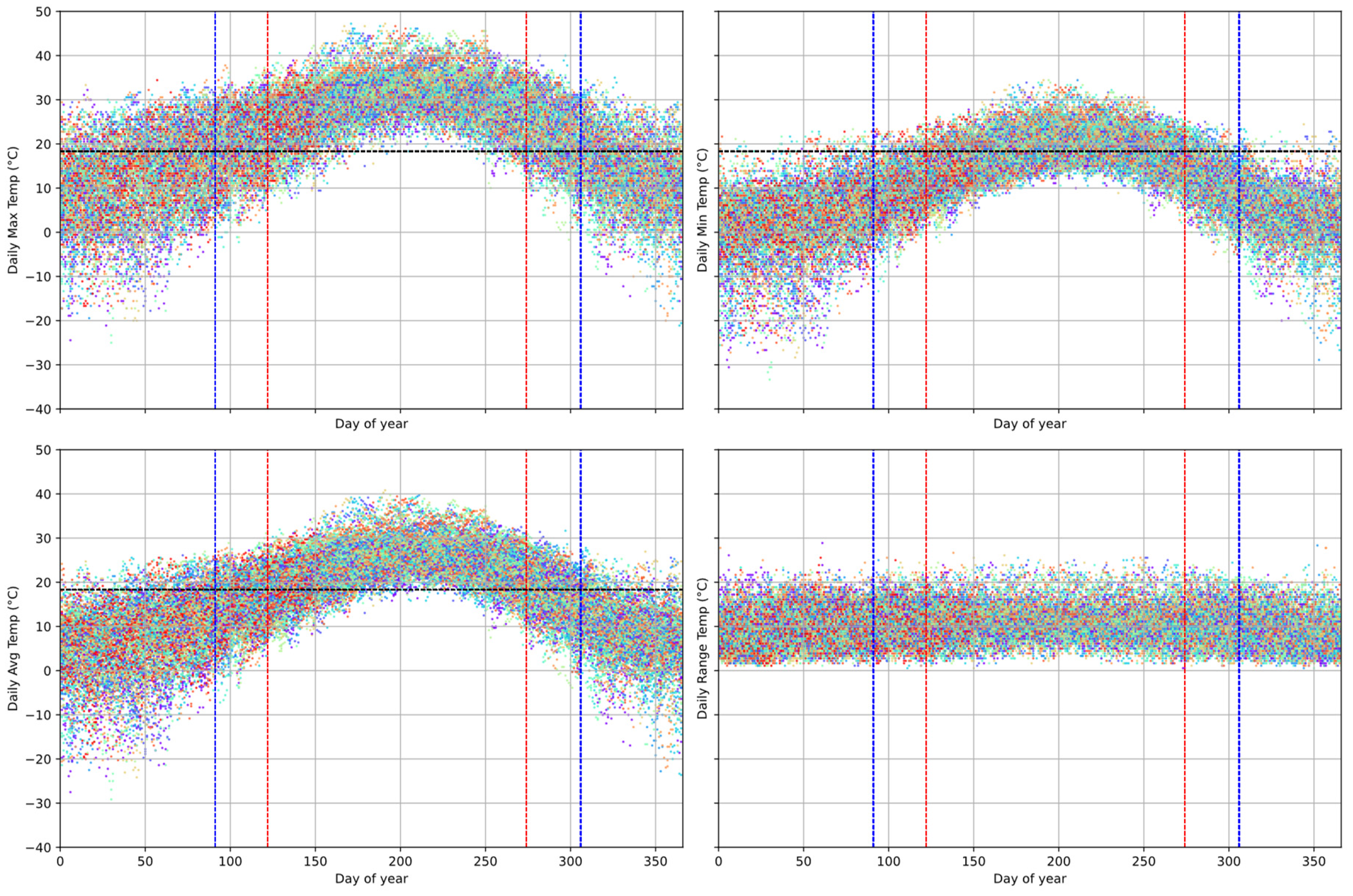
2.2. Temperature Data and Stylized Facts

Our analysis begins with daily maximum and minimum temperatures, sourced from Speedwell (CME’s official settlement data provider) for January 2014 through May 2024. Observations come from standardized airport monitoring stations to ensure consistency.
Figure 1 plots daily maximum, minimum, average, and range against day-of-year over the 2014–2024 period. Each panel exhibits pronounced seasonality: average temperatures peak mid-summer and bottom out mid-winter. Winter months display a wider vertical spread in both maximum and minimum values, indicating elevated volatility, whereas summer months display tighter clustering. The daily temperature range remains right-skewed year-round, with frequent small ranges punctuated by occasional large spikes, implying sporadic intraday extremes. These stylized facts, pronounced seasonality, volatility clustering, and skewed tails, motivate a two-stage baseline model that captures deterministic patterns and time-varying volatility before analyzing residual extremes and dependencies [11,18,27].

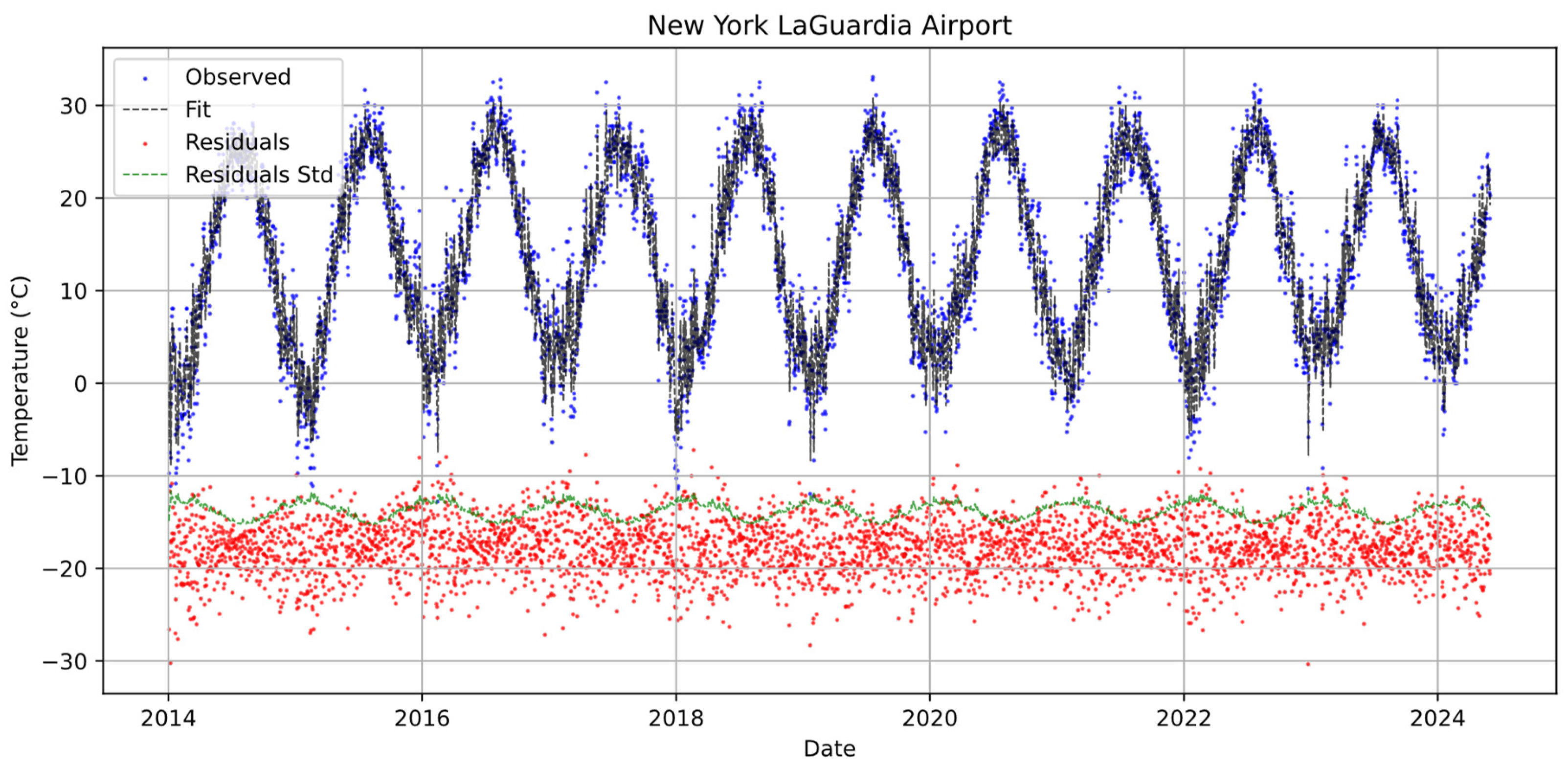
2.3. Baseline Temperature Modeling

To isolate stochastic fluctuations for EVT and dependence analyses, we adopt a two-stage model that first captures deterministic mean and seasonal components, then models conditional variance.

2.3.1. Conditional Mean

Let T t denote the observed daily average temperature for a given city on day t. We model its conditional mean T ^ t using an ARMAX specification:
ϕ ( L ) T t β 0 + β 1 t + A 1 sin 2 π d t + A 2 cos 2 π d t = θ ( L ) ε t
ϕ ( L ) = 1 ϕ 1 L ϕ p L p
θ ( L ) = 1 + θ 1 L + + θ q L q
ε t N 0 , σ t 2
where d t [ 0 , 1 ] is the fractional day-of-year, β 0 and β 1 capture intercept and linear trend, A 1 , A 2 are seasonal amplitudes, and L denotes the lag operator. The orders p , q { 0 , 1 , 2 } are selected by Akaike information criterion (AIC). Coefficients ( β 0 , β 1 , A 1 , A 2 ) and ARMA parameters ( ϕ i , θ j ) are estimated via Maximum Likelihood Estimation (MLE). Preliminary diagnostics on residuals ε t = T t T ^ t reveal remaining seasonality and volatility clustering, necessitating a conditional variance model (see Figure 2).

2.3.2. Seasonal GARCH Conditional Variance

To capture the observed volatility clustering and seasonal variance patterns, the residuals ε t are modeled via a Seasonal-GARCH(1, 1) with harmonic terms [18,28,29]:
σ t 2 = ω + α ε t 1 2 + β σ t 1 2 + A 3 sin ( 2 π d t ) + A 4 cos ( 2 π d t )
where ω , α , β > 0 , α + β < 1 (stationarity), and A 3 , A 4 capture seasonal variance effects. Parameters ( ω , α , β , A 3 , A 4 ) are estimated via MLE, subject to ω 2 > A 3 2 + A 4 2 and σ t 2 > 0 (variance nonnegativity) [30].
Table 1 reports RMSE , R 2 , AIC, and diagnostic p-values (Ljung-Box for residuals and squared residuals, ARCH-LM). No Ljung-Box or ARCH-LM test rejects white noise, confirming negligible remaining autocorrelation or ARCH effects. Consequently, the standardized residuals ε t , T (Equation (9)) are approximately i.i.d. and suitable for EVT and dependence modeling.
Figure 2 illustrates this decomposition for New York LaGuardia Airport: the observed series, fitted mean, residuals, and estimated conditional standard deviation.
ε t , T = T t T ^ t σ ^ t
ε t , H D D = max ( 0 , 65   ° F T t ) max ( 0 , 65   ° F T ^ t ) σ ^ t
ε t , C D D = max ( 0 , T t 65   ° F ) max ( 0 , T ^ t 65   ° F ) σ ^ t

2.4. Extracting HDD/CDD Residuals

The index residuals for HDD and CDD on day t are defined in Equations (10) and (11). These index residuals preserve time-varying volatility while reflecting the nonlinear truncation inherent in degree-day measures. This baseline modeling framework, filtering deterministic trends, seasonality, and conditional heteroskedasticity, prepares the residual series for focused EVT and copula-based dependence analyses in subsequent sections.

3. Univariate Tail Behavior in HDD/CDD Instruments

Standard deviation and other central-moment measures capture dispersion but are inadequate for quantifying extreme-event risk in heavy-tailed distributions. In weather derivatives, rare but severe deviations, such as an unseasonably warm winter that dramatically reduces an HDD payout, can generate disproportionate losses. Accordingly, we employ the Extreme Value Index (EVI), denoted ξ , which characterizes the decay rate of a distribution’s tail. A Gaussian or exponential distribution has ξ = 0 , while a positive ξ indicates a heavy (Pareto-type) tail. Larger ξ correspond to slower decay of probability density in tails and higher likelihood of extreme realizations [20,31,32,33].
Starting from our two-stage baseline model in Section 2.3, we compute standardized residuals from Section 2.4. The Equation (10) isolates the stochastic component of the realized HDD value relative to its predicted counterpart, while Equation (11) isolates the CDD residual.

3.1. Estimating the Extreme Value Index

For each of the 13 cities, we estimate the EVI ξ separately for the left (lower) and right (upper) tails of each standardized residual series { ε t , T } , { ε t , H D D } , { ε t , C D D } . We employ the Schultze-Steinebach estimator to each tail since it is ranked among the top performers in a comprehensive benchmarking study for moderate-size samples [34,35].
Figure 3 displays the estimated left- and right-tail EVI across all 13 cities. The left three columns correspond to tail risks under extreme heat, while the right three columns correspond to tail risks under extreme cold.

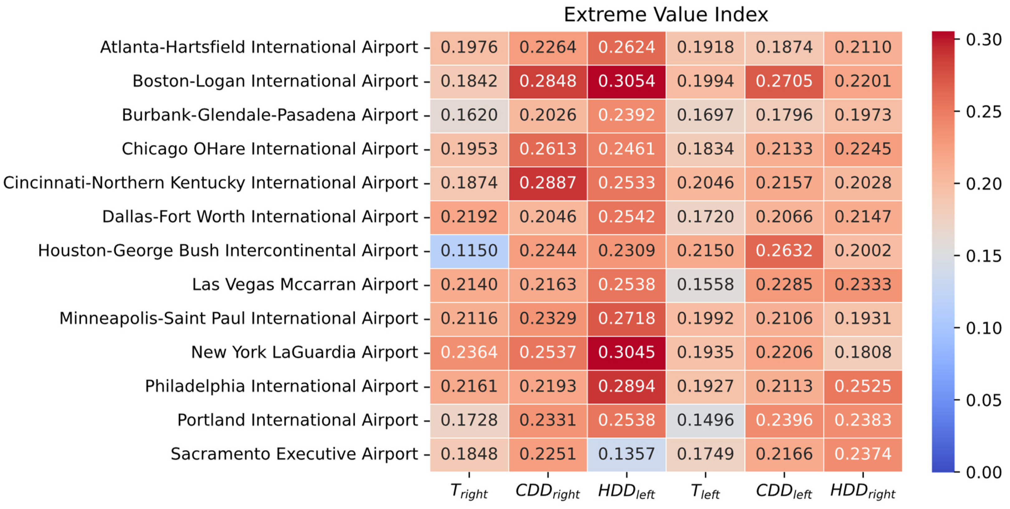
3.2. Aggregate EVI Summary

The average EVI in descending order is: ξ ¯ HDD , left ( 0.254 ) > ξ ¯ CDD , right ( 0.236 ) > ξ ¯ CDD , left ( 0.220 ) > ξ ¯ HDD , right ( 0.216 ) > ξ ¯ T , right ( 0.192 ) > ξ ¯ T , left ( 0.185 ) . Several insights follow:
1.
Degree-Day Amplification of Tail Risk. Both HDD and CDD residuals exhibit heavier tails ( ξ ¯ > 0.21 ) than temperature residuals ( ξ ¯ 0.19 ). This amplification arises because degree days apply a nonlinear transformation and truncate negative values at zero, concentrating more probability mass into extreme payout-relevant outcomes.
2.
Asymmetry of Left vs. Right Tails.
  • For HDD, ξ ¯ HDD , left = 0.254 (warm-winter shocks) exceeds ξ ¯ HDD , right = 0.216 (cold-winter shocks). Warm winters, which drastically reduce HDD payouts, are more heavy-tailed than cold shocks.
  • For CDD, ξ ¯ CDD , right = 0.236 (hot-summer shocks) exceeds ξ ¯ CDD , left = 0.220 (cool-summer shocks), indicating that extreme heat events are marginally more heavy-tailed than extreme cooling events in summer.
3.
Spatial Variation in Tail Thickness.
  • Northern cities (Minneapolis, Chicago, New York, Boston, Philadelphia, Cincinnati) exhibit the highest ξ ^ HDD , left [ 0.246 , 0.305 ] , indicating that unexpectedly warm winters in colder climates produce the most extreme heavy-tailed outcomes.
  • Southern/Western cities (Houston, Atlanta, Las Vegas, Sacramento, Portland, Burbank) exhibit lower ξ ^ HDD , left [ 0.136 , 0.262 ] , meaning warm-winter shocks in milder climates are less heavy-tailed than those in the North.

3.3. Practical Implications

Our analysis reveals that long HDD positions face the heaviest tail risk (warm-winter shocks), followed by short CDD positions (hot-summer shocks), while counterparties on the opposite sides incur comparatively lighter-tailed losses. Trading and risk-management decisions, such as setting initial margins, structuring hedges, and allocating capital reserves, should explicitly integrate city-specific EVI parameters rather than rely on the symmetric Gaussian or thin-tailed assumptions.
Moreover, the spatial heterogeneity of ξ underscores that tail risk varies substantially across regions. Exchanges and clearinghouses could calibrate initial and variation margins by referencing each city’s estimated ξ . Similarly, traders seeking to hedge warm-winter risk might short HDD contracts in northern cities and long HDD futures in southern cities, exploiting north-south disparity in tail heaviness. Finally, financial institutions holding long HDD positions may provision capital in line with tail probabilities implied by ξ . Under a heavy tail with ξ = 0.254 , a 1-in-1000 warm-winter event is far more probable than under a Gaussian model, requiring substantially larger capital buffers to cover potential extreme losses.

4. Cross-Location Extremes: Multivariate Tail Dependence in HDD/CDD Residuals

Multivariate extreme analysis uncovers how concurrent extreme weather events across multiple locations co-occur. For a portfolio holding HDD or CDD contracts across different cities, joint tail occurrences can substantially erode the benefits of geographic diversification and magnify portfolio level losses. In this section, we introduce the Tail Dependence Coefficient (TDC), describe its nonparametric estimation, and present empirical TDC heatmaps for both HDD and CDD residuals. We then discuss the implications for diversification and risk management.

4.1. Tail Dependence Coefficient: Definition and Intuition

Let ( X 1 , X 2 ) denote a pair of standardized residuals (e.g., two cities’ HDD residuals). The Tail Dependence Coefficient (TDC) λ measures the probability that one variable is extreme given that the other is extreme, in the limit as we move far into the tail. Formally, for lower-tail (simultaneous “extremely small” values), we write:
λ = lim q 0 + P ( X 2 F 2 1 ( q ) | X 1 F 1 1 ( q ) )
where F i 1 ( q ) = inf { x R : F ( x ) q } is the q-quantile of X i . A positive λ indicates that as X 1 becomes very small (e.g., a large warm-winter HDD shock in one city), X 2 also has non-negligible probability of being very small. In practice, both negative-tail (warm-winter or cool-summer shocks) and positive-tail (cold-winter or hot-summer shocks) co-extremes matter, depending on whether one holds long or short positions. To capture all four tail quadrants (lower/upper extremes of both residuals), we employ a symmetrized version of λ .

4.2. Nonparametric Estimation of TDC

We adopt the non-parametric estimator proposed by Ferreira (Equation (12)) [36,37], which leverages the fact that tail dependence can be expressed via any rotation of a continuous copula. Denote by F ^ i ( x ) the empirical CDF of city i’s residuals. By taking the minimum among four rotated maxima, this estimator simultaneously captures both lower and upper tail dependence. The estimated TDC is:
λ ^ = 3 [ 1 min { u 1 , u 2 , u 3 , u 4 } ] 1 u 1 = 1 n i = 1 n max { F ^ 1 ( X 1 ( i ) ) , F ^ 2 ( X 2 ( i ) ) } u 2 = 1 n i = 1 n max { 1 F ^ 1 ( X 1 ( i ) ) , F ^ 2 ( X 2 ( i ) ) } u 3 = 1 n i = 1 n max { 1 F ^ 1 ( X 1 ( i ) ) , 1 F ^ 2 ( X 2 ( i ) ) } u 4 = 1 n i = 1 n max { 1 F ^ 2 ( X 2 ( i ) ) , F ^ 1 ( X 1 ( i ) ) }
Figure 4 and Figure 5 summarize estimated TDC λ ^ via heatmaps for HDD and CDD residuals across 13 U.S. cities. To assess estimation uncertainty, we implement a simple non-parametric bootstrap (500 replications) and derive standard deviation from the empirical distribution of { λ ^ } .

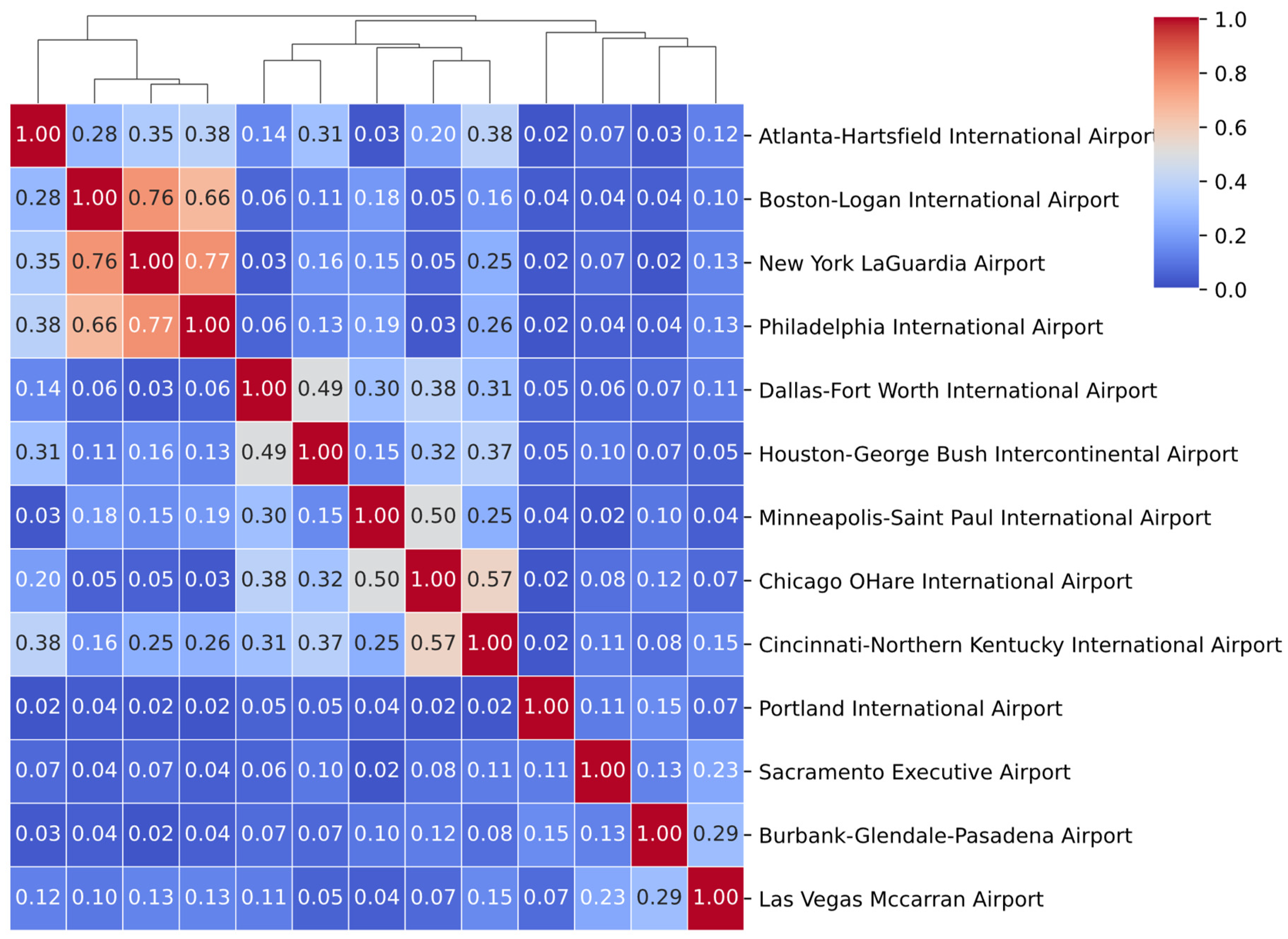
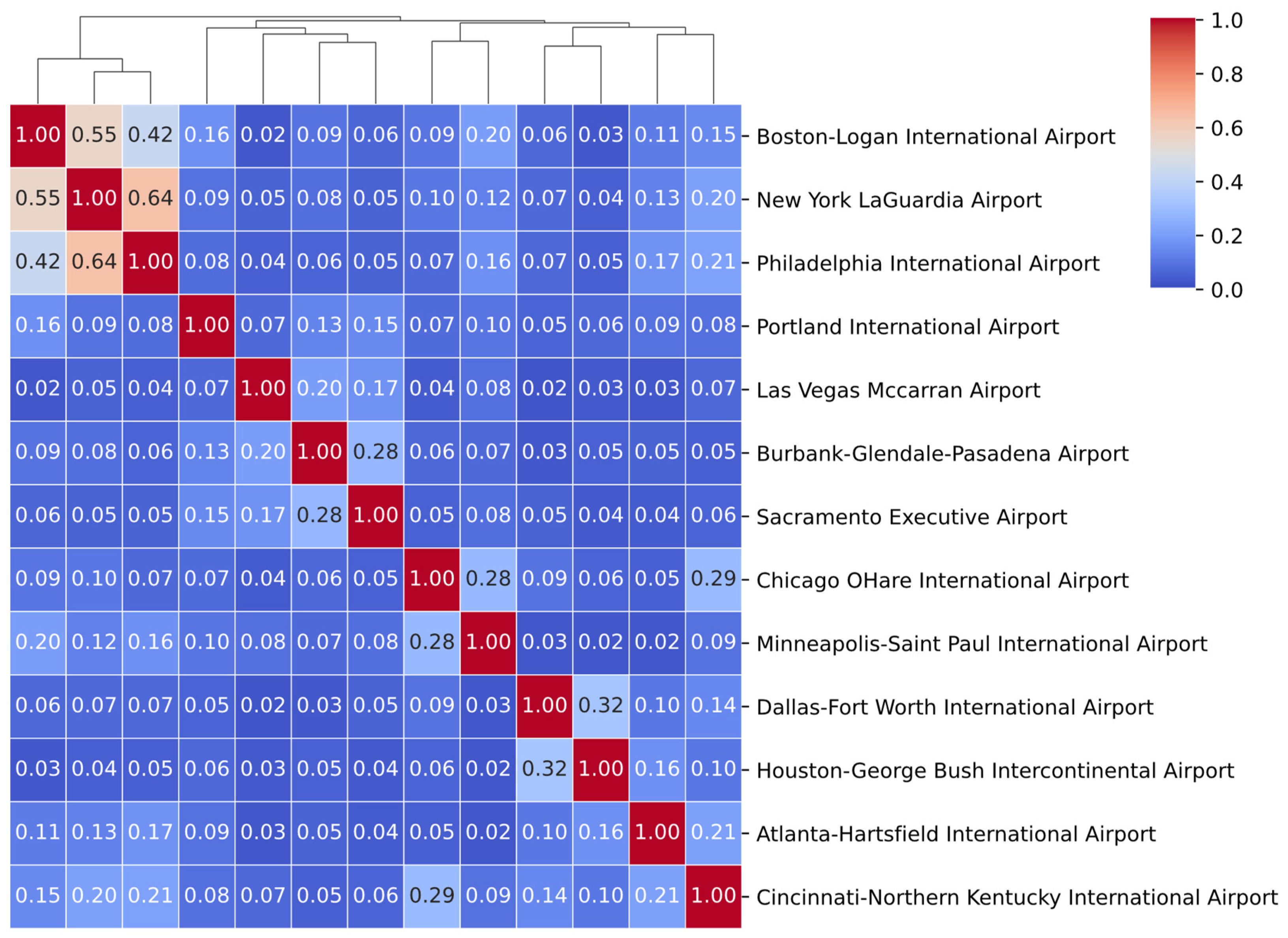
4.2.1. HDD Residuals (Figure 4)

Overall, λ ^ for HDD residuals range from 0.02 to 0.77 , indicating substantial tail co-extremes. The strongest tail dependence occurs among Notheast triplets (e.g., Boston-New York-Philadelphia), reflecting historical joint warm-winter and cold-winter episodes (e.g., the 2015 Northeast blizzards, the 2019 polar vortex, and the 2022 winter storm Elliott). The Midwest cluster (Minneapolis-Chicago) and South cluster (Houston-Dallas) each exhibit high λ ^ 0.50 . In contrast, cross-region pairs show much weaker λ ^ , indicating relative independence of extreme HDD shocks.

4.2.2. CDD Residuals (Figure 5)

CDD residuals exhibit generally lower λ ^ ranging from 0.02 to 0.64 . The strongest λ ^ occurs among Notheast pairs (e.g., Boston-New York-Philadelphia). Western pairs (e.g., Las Vegas-Sacramento) show moderate tail dependence, reflecting shared summer heat risks. Inter-regional pairs (e.g., Houston-Boston, Chicago-Las Vegas) have near-zero λ ^ < 0.05 , indicating limited co-extremes.

4.3. Practical Implications

A portfolio of HDD contracts concentrated in geographically proximate northern cities could face large joint extremes, limiting the benefits of diversification. Traders hedging warm-winter risk in the Northeast might offset by taking positions in lower-dependence southern or western markets.
CDD residuals show weaker tail dependence. Portfolios combining southern and western CDD exposures (e.g., Houston–Las Vegas) could have lower co-extreme risk, making diversification across climate zones more effective in summer scenarios.
By quantifying and visualizing joint tail dependence across locations, we demonstrate that joint extremes in HDD and CDD residuals vary markedly by region and season. In the following section, we incorporate these insights into copula-based portfolio simulations and joint VaR–ES backtests to evaluate the practical impact on risk forecasts.

5. Portfolio Risk Modeling with Copulas: Comparison and Backtesting

5.1. Candidate Copula Dependence Models

Market participants rarely hold a single weather-derivative contract in isolation. Instead, they build portfolios, often long or short positions in HDD or CDD futures across multiple cities, to hedge or speculate on spatially diversified weather risk.
Copula-based modeling provides a powerful and flexible framework for this task, enabling the separation of the marginal distribution of each individual weather risk from their joint dependence structure [38]. According to Sklar’s theorem, every multivariate joint distribution function can be expressed using its marginals and a copula function [39]. Let F be the be a joint distribution function with marginals F i ( x i ) . Then, there exists a copula function C such that for all x 1 , x 2 , , x n :
F ( x 1 , x 2 , , x n ) = C ( F 1 ( x 1 ) , F 2 ( x 2 ) , , F n ( x n ) )
The copula function C is unique if the marginal distribution functions are continuous. Conversely, the joint distribution can be reconstructed given a copula and marginal distributions. This allows us to explicitly model the complex interdependencies identified previously, without being restricted by the assumptions of simpler multivariate distributions. This separation enables risk managers and researchers to model tail dependencies explicitly, leading to more accurate risk assessments in areas such as credit risk, portfolio optimization, and systemic risk analysis [40].
In this section, we employ three widely used copula families to model the dependence between the standardized residuals ( ε t , T from Section 2.3) across the 13 US cities. Univariate marginals are modeled non-parametrically via their empirical CDFs, ensuring that the copula fit focuses purely on dependence.
Although Archimedean copulas such as Gumbel and Clayton can capture one-sided tail dependence using rotations, they impose full exchangeability and lack the flexibility needed to model the rich, asymmetric 13-dimensional dependence structure observed in our standardized temperature residuals. By contrast, the pair copula construction allows pair-specific bivariate copula modeling and asymmetric tail behavior. Therefore, we focus our comparison on Gaussian, Student’s t, and R-Vine families.

5.1.1. Gaussian Copula

With R [ 1 , 1 ] n × n being a n-variate correlation matrix, the multivariate copula distribution function C and copula density c are:
C ( u ; R ) = Φ d ( Φ 1 ( u 1 ) , , Φ 1 ( u n ) ; R ) , u ( 0 , 1 ) n
c ( u ; R ) = ϕ d ( Φ 1 ( u 1 ) , , Φ 1 ( u n ) ; R ) Π i = 1 d ϕ ( Φ 1 ( u i ) ) , u ( 0 , 1 ) n
where Φ ( x ) is the cumulative distributive function of the standard Gaussian distribution, ϕ ( x ) is the density function of the standard Gaussian distribution.
The Gaussian copula is an elliptical copula with zero TDC. It is known applied to credit derivatives and could be one of the reasons behind the global financial crisis of 2008 [41].

5.1.2. Student’s t Copula

With R [ 1 , 1 ] n × n being a n-variate correlation matrix together with a degrees of freedom ν > 0 , the multivariate copula distribution function C and copula density c are:
C ( u ; R , ν ) = T d , ν ( T 1 , ν 1 ( u 1 ) , , T 1 , ν 1 ( u n ) ; R ) , u ( 0 , 1 ) n
c ( u ; R , ν ) = t d , ν ( T 1 , ν 1 ( u 1 ) , , T 1 , ν 1 ( u n ) ; R ) Π i = 1 d t 1 , ν ( T 1 , ν 1 ( u i ) ) , u ( 0 , 1 ) n
where T 1 , ν ( x ) is the cumulative distributive function of the univariate t distribution with parameter ν > 0 , t 1 , ν ( x ) is the corresponding density function.
The Student’s t copula is an elliptical copula with symmetric tail dependence controlled by its degrees of freedom. It can capture moderate joint extremes but remains restrictive in higher dimensions.

5.1.3. Vine Copula

Focusing on dependence structures, consider the pair copula construction for a three-dimensional copula without marginals:
c ( u 0 , u 1 , u 2 ) = c 0 , 2 ; 1 ( C 0 | 1 ( u 0 | u 1 ) , C 2 | 1 ( u 2 | u 1 ) ) c 1 , 2 ( u 1 , u 2 ) c 0 , 1 ( u 0 , u 1 )
where c 0 , 2 ; 1 is the copula density associated with the conditional bivariate copula C 0 , 2 ; 1 ( u 0 , u 2 | u 1 ) = C 0 , 2 | 1 C 0 | 1 1 ( u 0 | u 1 ) , C 2 | 1 1 ( u 2 | u 1 ) | u 1 , which has a conditioned set { 0 , 2 } and a conditioning set { 1 } [42]. Here C 0 | 1 ( u 0 | u 1 ) and C 2 | 1 ( u 2 | u 1 ) are conditional distribution functions associated with bivariate copulas C 0 , 1 and C 1 , 2 , also known as h-functions and denoted as h 0 | 1 ; ( u 0 | u 1 ) = C 0 , 1 ( u 0 , u 1 ) u 1 and h 2 | 1 ; ( u 2 | u 1 ) = C 1 , 2 ( u 1 , u 2 ) u 1 [43]. The bivariate copula C 0 , 1 has a conditioned set { 0 , 1 } and a conditioning set ∅, while the bivariate copula C 1 , 2 has a conditioned set { 1 , 2 } and a conditioning set ∅. Here we adopt the simplifying assumption that c 0 , 2 ; 1 ( u 0 , u 2 ; x 1 ) = c 0 , 2 ; 1 ( u 0 , u 2 ) , indicating that the bivariate copula associated with conditional distributions does not depend on specific values of the conditioning variables [44].
The decomposition of a n-dimensional ( n 3 ) copula into a cascade of bivariate copulas is non-unique, but every possible decomposition can be represented by nested trees known as R-Vine [45]. Each vine structure corresponds to a different decomposition of the joint copula density, with each tree representing a connected, undirected, acyclic graph ( V k , E k ) , k { 0 , 1 , , D 2 } . Each vertex is a set of integers and each undirected edge connects two vertices.
Definition 1.
A collection of trees { ( V k , E k ) | k { 0 , 1 , , n 2 } } is a n-dimensional R-Vine on the set V 0 = { { 0 } , { 1 } , , { n 1 } } if:
1. 
( V 0 , E 0 ) is a spanning tree,
2. 
For k { 1 , , n 2 } , ( V k , E k ) is a spanning tree with vertices V k = { a b | { a , b } E k 1 , | a b | = k + 1 } , | V k | = n k , | E k | = n k 1 ,
3. 
(Proximity condition) Each undirected edge e = { a , b } E k connects vertices a , b V k where | a b | = k , | a b | = | ( a b ) ( a b ) | = 2 , withdenoting the symmetric difference.
Definition 2.
A vine copula { ( V k , E k , C k ) | k { 0 , 1 , , D 2 } } attach a bivariate copula to each undirected edge of an R-Vine. For each undirected edge e = { a , b } E k :
1. 
The conditioning set of e is a b with | a b | = k ,
2. 
The conditioned set of e is a b with | a b | = 2 . The elements of this bivariate set a b are denoted v l , v r where v l < v r ,
3. 
The bivariate copula attached to e is C v l , v r ; a b C k ,
4. 
The corresponding conditional distribution functions (h-functions) are h v l | v r ; a b ( u 0 | u 1 ) = u 1 C v l , v r ; a b ( u 0 , u 1 ) and h v r | v l ; a b ( u 1 | u 0 ) = u 0 C v l , v r ; a b ( u 0 , u 1 ) .
Vine copulas, built upon flexible pair-copula constructions, offer an approach for modeling complex, high-dimensional dependencies. Their structure allows for the capture of features such as asymmetry and varying tail dependence patterns across different variable pairs [43], making them particularly well-suited for the intricate dependencies often observed in meteorological data [46] and financial returns [47,48]. By decomposing the multivariate dependence into a cascade of bivariate conditional copulas, vine copulas provide a scalable approach that balances model flexibility with parameter parsimony. Detailed reviews of vine copulas are available in [42,49,50]. In this study we use the classical Dissmann’s algorithm for vine copula fitting [51], and use non-parametric (transformation local likelihood) bivariate copula for its proven flexibility and efficiency in a comprehensive study [52]. By convention, We adopt the simplifying assumption that conditional copulas do not vary with the conditioning variable [53].

5.2. Copula Model Evaluation via Portfolio Backtesting

5.2.1. Portfolio Setup and Cross-Validation Framework

We evaluate three copula families by their ability to forecast daily portfolio VaR0.05 and ES0.05. To reflect common hedging practices, we form two equally weighted portfolios across the same 13 cities:
  • Long HDD Portfolio: A $ 1 long position in each city’s HDD index future.
  • Long CDD Portfolio: A $ 1 long position in each city’s CDD index future.
We use the repeated 5-fold cross-validation over the full sample (January 2014–May 2024), with 100 random train-validation splits. Each split proceeds as follows:
1.
Fit Marginals (Training Set). For each city, fit the empirical CDF of the standardized residuals { ε t , T } from our baseline model (Section 2.3).
2.
Transform to Uniforms. Map each city’s training residuals to pseudo-observations u i , t = F ^ i ( ε i , t , T ) [ 0 , 1 ] .
3.
Fit Copula (Training Set). Estimate the copula on the multivariate uniform data:
  • For Gaussian and Student’s t, estimate the correlation matrix (and degrees of freedom).
  • For R-Vine, sequentially fit the non-parametric bivariate copula inside vine copula using Dissmann’s algorithm [51,52].
4.
Simulate Portfolio Losses (Validation Set). For each day t in the validation fold:
(a)
Draw large number of samples from the fitted copula.
(b)
Invert the empirical CDFs to obtain simulated standardized residuals for each city i.
(c)
Compute each city’s simulated HDD (or CDD) index values by adding the simulated standardized residuals to the baseline prediction from Section 2.3, then form the equally weighted portfolio value based on simulated index for day t.
(d)
Estimate VaRα=0.05 and ESα=0.05 of the portfolio.
Across the 100 splits, we collect all out-of-sample VaRα=0.05, ESα=0.05, and realized daily portfolio P&L X t .

5.2.2. Joint VaR-ES Backtest

We apply the joint VaR-ES backtest [54]. At each day t, denote:
Z t = α ( E S α , t V a R α , t ) + ( X t + V a R α , t ) 1 { X t + V a R α , t 0 }
Z = t = 1 T Z t T
where α = 0.05 , X t is the realized portfolio P&L (negative if a loss). The Z is a scoring function that merit from a model comparison perspective. Under correct joint VaR/ES specification, Z is close to 0 which indicates accurate joint tail forecasts; positive Z signals systematic overestimation of tail risk, while negative Z signals underestimation. Concretely, a moderately large positive Z tells us that our model is too conservative (we’re holding more capital than needed), whereas a negative Z warns of potential under-provisioning and higher surprise losses. The test is known for its robustness and its prudential nature: it penalizes underestimation of risk more heavily than overestimation.
Because we repeat 5-fold cross-validation 100 times, each model yields 100 “out-of-sample” Z values; Table 2 shows their average and two-standard-deviation band. Repeated cross-validation with the joint VaR–ES backtest ensures robust model comparison. Reporting the mean ± 2 std deviation of Z highlights not only average performance but also variation across data splits, helping risk managers quantify model uncertainty.
For CDD portfolio, all three copulas produce Z statistics close to 0, indicating that even a simple Gaussian copula suffices to capture the relatively weak tail dependence. The Student–t copula has lower mean Z. The R-Vine model’s Z 0.00009 is the lowest. Thus, for CDD portfolios, where empirical TDC rarely exceed 0.30 , the additional flexibility of Student–t or R-Vine yields some improvements over the Gaussian copula.
For HDD portfolio, by contrast, the HDD portfolio backtest highlights the necessity of a flexible dependence model. Gaussian and Student–t copulas both yield Z > 0.0012 , significantly above zero (more than 40 standard errors), indicating systematic overestimation of joint tail losses. This overestimation arises because both elliptical copulas cannot reproduce the strong, geographically clustered tail dependence observed among HDD residuals (Section 4). In contrast, the R-Vine copula achieves Z 0.00009 , essentially closer to zero, confirming the highly flexible pair-copula construction reaches the best performance in modeling the tail risk of HDD exposures.

5.3. Practical Implications

The R-Vine copula’s near-zero Z confirms its ability to reproduce the complex, regionally concentrated tail dependence among HDD/CDD residuals. Practitioners hedging a basket of HDD/CDD positions could adopt a vine-based copula to avoid consistent overestimation (or underestimation) of risk.
In sum, the backtesting exercise confirms that while simpler elliptical copulas may suffice for CDD portfolios, accurate modeling of HDD portfolio tail risk requires the flexibility of an R-Vine construction. This ensures practitioners can set margins and capital reserves in line with empirical co-extreme probabilities and avoid systematic mispricing of joint tail exposures.

6. Conclusions

Standard approaches to weather-derivative risk, relying on Gaussian assumptions and simple dependence structures, fail to account for the heavy-tailed behavior and spatially heterogeneous co-extremes evident in temperature data. In this paper, we develop a unified framework that (i) filters trend, seasonality, and conditional heteroskedasticity via a two-stage ARMAX–Seasonal GARCH model; (ii) employs EVI to measure univariate tail thickness of HDD and CDD residuals; (iii) uses TDC to reveal geographically clustered extremes; and (iv) integrates these insights into a joint VaR–ES backtest, demonstrating that only the flexible R-Vine copula can faithfully reproduce the joint tail risk of HDD portfolios.
Empirically, residuals of degree-day indices exhibit markedly heavier tails than raw temperature shocks, with warm-winter HDD events in northern cities standing out as most extreme. Tail-dependence analysis highlights strong clustering among geographically proximate markets (e.g., Boston–New York–Philadelphia), whereas CDD residuals display weaker, more diffuse co-extremes. In portfolio simulations, Gaussian and Student’s t copulas systematically misestimate HDD tail risk, whereas an R-Vine construction captures the intricate, region-specific co-extremes and yields accurate out-of-sample VaR and ES.
These findings carry two implications for practitioners. First, margin and capital requirements based on elliptical copulas may be fundamentally misaligned with observed joint-extreme frequencies, especially for HDD contracts. Second, a R-Vine copula approach, separating empirical marginals from their complex tail-dependence structure, enables more reliable risk forecasts, better-calibrated initial and variation margins, and capital reserves consistent with actual co-extreme probabilities.
Looking ahead, it would be valuable to (a) develop dynamic copula models that allow tail dependence to evolve over time, perhaps in response to climate trends; (b) incorporate downscaled climate scenarios into marginal and dependence forecasts; (c) extend this framework to non-U.S. markets or other weather indices (e.g., rainfall, wind); and (d) optimize portfolio construction under these refined risk measures, thereby guiding real-world hedging in energy, agriculture, and other weather-sensitive sectors.

Author Contributions

Conceptualization, T.C. and K.C.; methodology, T.C.; software, T.C.; validation, S.R.P.; resources, K.C.; writing—original draft preparation, S.R.P. and T.C.; writing—review and editing, T.C., S.R.P. and K.C.; funding acquisition, K.C. All authors have read and agreed to the published version of the manuscript.

Funding

This research received no external funding.

Institutional Review Board Statement

Not applicable.

Informed Consent Statement

Not applicable.

Data Availability Statement

Restrictions apply to the availability of these data. The original temperature data were obtained from Speedwell Climate Ltd under a proprietary academic-use agreement and are not publicly available.

Conflicts of Interest

The authors declare no conflicts of interest.

References

  1. Kikstra, J.S.; Nicholls, Z.R.; Smith, C.J.; Lewis, J.; Lamboll, R.D.; Byers, E.; Sandstad, M.; Meinshausen, M.; Gidden, M.J.; Rogelj, J.; et al. The IPCC Sixth Assessment Report WGIII climate assessment of mitigation pathways: From emissions to global temperatures. Geosci. Model Dev. 2022, 15, 9075–9109. [Google Scholar] [CrossRef]
  2. Hermann, M.; Wernli, H.; Röthlisberger, M. Drastic increase in the magnitude of very rare summer-mean vapor pressure deficit extremes. Nat. Commun. 2024, 15, 7022. [Google Scholar] [CrossRef] [PubMed]
  3. Sutton-Vermeulen, D. Managing climate risk with CME Group weather futures and options. CME Group 2021, 20, 2021. [Google Scholar]
  4. Bemš, J.; Aydin, C. Introduction to weather derivatives. WIREs Energy Environ. 2022, 11, e426. [Google Scholar] [CrossRef]
  5. Prentzas, A.; Bournaris, T.; Nastis, S.; Moulogianni, C.; Vlontzos, G. Enhancing Sustainability through Weather Derivative Option Contracts: A Risk Management Tool in Greek Agriculture. Sustainability 2024, 16, 7372. [Google Scholar] [CrossRef]
  6. Neal, T.; Newell, B.R.; Pitman, A. Reconsidering the macroeconomic damage of severe warming. Environ. Res. Lett. 2025, 20, 044029. [Google Scholar] [CrossRef]
  7. Stulec, I.; Petljak, K.; Bakovic, T. Effectiveness of weather derivatives as a hedge against the weather risk in agriculture. Agric. Econ./Zemědělská Ekon. 2016, 62, 356–362. [Google Scholar] [CrossRef]
  8. Bressan, G.M.; Romagnoli, S. Climate risks and weather derivatives: A copula-based pricing model. J. Financ. Stab. 2021, 54, 100877. [Google Scholar] [CrossRef]
  9. The Straits Times. Use of Weather Derivatives Surges as Extreme Climate Events Rock the Globe. 2023. Available online: https://www.straitstimes.com/world/europe/use-of-weather-derivatives-surges-as-extreme-climate-events-rock-the-globe (accessed on 14 May 2025).
  10. Benth, F.E.; Härdle, W.K.; Cabrera, B.L. Pricing of Asian temperature risk. In Statistical Tools for Finance and Insurance; Cizek, P., Härdle, W.K., Weron, R., Eds.; Springer: Berlin/Heidelberg, Germany, 2011; pp. 163–199. [Google Scholar] [CrossRef]
  11. Alaton, P.; Boualem, D.; Stillberger, D. On modelling and pricing weather derivatives. Appl. Math. Financ. 2002, 9, 1–20. [Google Scholar] [CrossRef]
  12. Alfonsi, A.; Vadillo, N. A stochastic volatility model for the valuation of temperature derivatives. IMA J. Manag. Math. 2024, 35, 737–785. [Google Scholar] [CrossRef]
  13. Blanco, S.S. Local sensitivity analysis of heating degree day and cooling degree day temperature derivative prices. Quant. Financ. 2025, 25, 653–670. [Google Scholar] [CrossRef]
  14. Benth, F.E.; Šaltytė Benth, J.; Koekebakker, S. Putting a Price on Temperature. Scand. J. Stat. 2007, 34, 746–767. [Google Scholar] [CrossRef]
  15. Benth, F.E.; Benth, J.š. The volatility of temperature and pricing of weather derivatives. Quant. Financ. 2007, 7, 553–561. [Google Scholar] [CrossRef]
  16. Benth, F.E.; Šaltytė Benth, J. Weather Derivatives and Stochastic Modelling of Temperature. Int. J. Stoch. Anal. 2011, 2011, 576791. [Google Scholar] [CrossRef]
  17. Benth, F.E.; Lempa, J. Hedging temperature risk with CDD and HDD temperature futures. Appl. Stoch. Model. Bus. Ind. 2024, 40, 1484–1497. [Google Scholar] [CrossRef]
  18. Campbell, S.D.; Diebold, F.X. Weather Forecasting for Weather Derivatives. J. Am. Stat. Assoc. 2005, 100, 6–16. [Google Scholar] [CrossRef]
  19. Šaltytė Benth, J.; Benth, F.E. A critical view on temperature modelling for application in weather derivatives markets. Energy Econ. 2012, 34, 592–602. [Google Scholar] [CrossRef]
  20. Embrechts, P.; Klüppelberg, C.; Mikosch, T. Modelling Extremal Events; Springer: Berlin/Heidelberg, Germany, 1997. [Google Scholar] [CrossRef]
  21. Erhardt, R.J.; Smith, R.L. Weather Derivative Risk Measures for Extreme Events. N. Am. Actuar. J. 2014, 18, 379–393. [Google Scholar] [CrossRef]
  22. de Haan, L.; Tank, A.K.; Neves, C. On tail trend detection: Modeling relative risk. Extremes 2015, 18, 141–178. [Google Scholar] [CrossRef]
  23. Carney, M.; Holland, M.; Nicol, M.; Tran, P. Runs of extremes of observables on dynamical systems and applications. Phys. D Nonlinear Phenom. 2024, 460, 134093. [Google Scholar] [CrossRef]
  24. Koh, J.; Steinfeld, D.; Martius, O. Using spatial extreme-value theory with machine learning to model and understand spatially compounding extremes. arXiv 2024, arXiv:2401.12195. [Google Scholar] [CrossRef]
  25. Chicago Mercantile Exchange. CME Degree Days Index Futures Rulebook. 2024. Available online: https://www.cmegroup.com/rulebook/CME/ (accessed on 5 April 2025).
  26. CME Group. CME Group Weather Suite Expanded. 2023. Available online: https://www.cmegroup.com/articles/2023/cme-group-weather-suite-expanded.html (accessed on 14 May 2025).
  27. Alexandridis K., A.; Zapranis, A.D. Weather Derivatives: Modeling and Pricing Weather-Related Risk; Springer: New York, NY, USA, 2013. [Google Scholar] [CrossRef]
  28. Engle, R.F. Autoregressive Conditional Heteroscedasticity with Estimates of the Variance of United Kingdom Inflation. Econometrica 1982, 50, 987–1007. [Google Scholar] [CrossRef]
  29. Engle, R.F.; Bollerslev, T. Modelling the persistence of conditional variances. Econom. Rev. 1986, 5, 1–50. [Google Scholar] [CrossRef]
  30. Esunge, J.; Njong, J.J. Weather derivatives and the market price of risk. J. Stoch. Anal. 2020, 1, 7. [Google Scholar] [CrossRef]
  31. Kelly, B.; Jiang, H. Tail Risk and Asset Prices. Rev. Financ. Stud. 2014, 27, 2841–2871. [Google Scholar] [CrossRef]
  32. McNeil, A.J.; Frey, R.; Embrechts, P. Quantitative Risk Management: Concepts, Techniques and Tools—Revised Edition; Princeton University Press: Princeton, NJ, USA, 2015. [Google Scholar]
  33. Chen, K.; Cheng, T. Measuring tail risks. J. Financ. Data Sci. 2022, 8, 296–308. [Google Scholar] [CrossRef]
  34. Schultze, J.; Steinebach, J. On least squares estimates of an exponential tail coefficient. Stat. Risk Model. 1996, 14, 353–372. [Google Scholar] [CrossRef]
  35. Fedotenkov, I. A Review of More than One Hundred Pareto-Tail Index Estimators. Statistica 2020, 80, 245–299. [Google Scholar] [CrossRef]
  36. Ferreira, M. Nonparametric Estimation of the Tail-Dependence Coefficient. REVSTAT-Stat. J. 2013, 11, 1–16. [Google Scholar] [CrossRef]
  37. Sohkanen, P. Estimation of the Tail Dependence Coefficient. Master’s Thesis, University of Helsinki, Helsinki, Finland, 2021. [Google Scholar]
  38. Lei, Z.; Li, P.; Wang, Y. The effect of compound heat-drought risk on municipal corporate bonds pricing: Evidence from China. N. Am. J. Econ. Financ. 2025, 79, 102462. [Google Scholar] [CrossRef]
  39. Sklar, M. Fonctions de répartition à n dimensions et leurs marges. In Annales de l’ISUP; Publications de l’Institut Statistique de l’Université de Paris: Paris, France, 1959; Volume 8, pp. 229–231. [Google Scholar]
  40. Jia, S.; Chen, X.; Han, L.; Jin, J. Global climate change and commodity markets: A hedging perspective. J. Futur. Mark. 2023, 43, 1393–1422. [Google Scholar] [CrossRef]
  41. Li, D.X. On Default Correlation: A Copula Function Approach. J. Fixed Income 2000, 9, 43–54. [Google Scholar] [CrossRef]
  42. Czado, C. Analyzing Dependent Data with Vine Copulas: A Practical Guide with R; Lecture Notes in Statistics Series; Springer International Publishing: Cham, Switzeralnd, 2019; Volume 222. [Google Scholar] [CrossRef]
  43. Aas, K.; Czado, C.; Frigessi, A.; Bakken, H. Pair-copula constructions of multiple dependence. Insur. Math. Econ. 2009, 44, 182–198. [Google Scholar] [CrossRef]
  44. Wattanawongwan, S.; Mues, C.; Okhrati, R.; Choudhry, T.; So, M.C. Modelling credit card exposure at default using vine copula quantile regression. Eur. J. Oper. Res. 2023, 311, 387–399. [Google Scholar] [CrossRef]
  45. Bedford, T.; Cooke, R.M. Vines–A new graphical model for dependent random variables. Ann. Stat. 2002, 30, 1031–1068. [Google Scholar] [CrossRef]
  46. Sommer, E.; Bax, K.; Czado, C. Vine Copula based Portfolio Level Conditional Risk Measure Forecasting. Econom. Stat. 2023. [CrossRef]
  47. Cheng, T.; Chen, K. A general framework for portfolio construction based on generative models of asset returns. J. Financ. Data Sci. 2023, 9, 100113. [Google Scholar] [CrossRef]
  48. Cheng, T. torchvinecopulib: Yet Another Vine Copula Package, Using PyTorch. 2024. Available online: https://zenodo.org/records/13901533 (accessed on 10 June 2025).
  49. Joe, H. Dependence Modeling with Copulas; Chapman and Hall/CRC: New York, NY, USA, 2014. [Google Scholar] [CrossRef]
  50. Czado, C.; Nagler, T. Vine Copula Based Modeling. Annu. Rev. Stat. Its Appl. 2022, 9, 453–477. [Google Scholar] [CrossRef]
  51. Dissmann, J.; Brechmann, E.C.; Czado, C.; Kurowicka, D. Selecting and estimating regular vine copulae and application to financial returns. Comput. Stat. Data Anal. 2013, 59, 52–69. [Google Scholar] [CrossRef]
  52. Nagler, T.; Schellhase, C.; Czado, C. Nonparametric estimation of simplified vine copula models: Comparison of methods. Depend. Model. 2017, 5, 99–120. [Google Scholar] [CrossRef]
  53. Nagler, T. Simplified vine copula models: State of science and affairs. Risk Sciences 2025, 1, 100022. [Google Scholar] [CrossRef]
  54. Deng, K.; Qiu, J. Backtesting expected shortfall and beyond. Quant. Financ. 2021, 21, 1109–1125. [Google Scholar] [CrossRef]
Figure 1. Daily maximum (top-left), minimum (top-right), average (bottom-left), and range (bottom-right) temperatures plotted against day-of-year for 13 U.S. cities (2014–2024). Dots are shaded on a blue-to-red gradient by year (blue = early sample years, red = most recent years). Red and blue vertical lines indicate Heating Degree Day (HDD) and Cooling Degree Day (CDD) contract windows, respectively. The black line marks the 65   ° F ( 18.33   ° C ) reference.
Commodities 04 00011 g001
Figure 2. Baseline temperature model for New York LaGuardia Airport: observed series, fitted mean, residuals, and conditional standard deviation.
Commodities 04 00011 g002
Figure 3. Extreme Value Index (EVI) estimates ξ ^ (left and right tails) of temperature residuals ε t , T , HDD residuals ε t , H D D , and CDD residuals ε t , C D D across 13 U.S. cities. Higher values indicate heavier tails. The left three columns correspond to tail risks under extreme heat, while the right three columns correspond to tail risks under extreme cold.
Commodities 04 00011 g003
Figure 4. Tail Dependence Coefficient (TDC) of HDD residuals across 13 stations in the US. Adjacent dendrogram shows hierarchical clustering. Bootstrap-based 2 std dev average 0.010 .
Commodities 04 00011 g004
Figure 5. Tail Dependence Coefficient (TDC) of CDD residuals across 13 stations in the US. Adjacent dendrogram shows hierarchical clustering. Bootstrap-based 2 std dev average 0.007 .
Commodities 04 00011 g005
Table 1. Baseline model goodness-of-fit by station: RMSE , R 2 , AIC, Ljung-Box on residuals and squared residuals, and ARCH-LM.
StationRMSE R 2 AICLB (10)LB (30)LB2 (10)LB2 (30)ARCH LM (10)
Atlanta-Hartsfield International Airport2.450.9021,852.8710.22 (0.42)30.94 (0.42)11.56 (0.32)25.90 (0.68)14.23 (0.16)
Boston-Logan International Airport3.140.8924,503.594.25 (0.94)13.58 (1.00)8.05 (0.62)26.94 (0.63)5.84 (0.83)
Burbank-Glendale-Pasadena Airport1.730.8920,098.878.56 (0.57)25.23 (0.71)10.47 (0.40)23.75 (0.78)14.74 (0.14)
Chicago O’Hare International Airport3.250.9124,554.502.24 (0.99)10.83 (1.00)6.12 (0.80)33.91 (0.28)8.03 (0.63)
Cincinnati-Northern Kentucky International Airport3.190.9024,011.254.81 (0.90)13.28 (1.00)4.63 (0.91)21.99 (0.85)4.76 (0.91)
Dallas-Fort Worth International Airport2.960.8923,344.2913.01 (0.22)38.21 (0.14)5.37 (0.87)18.62 (0.95)7.07 (0.72)
Houston-George Bush Intercontinental Airport2.650.8722,238.6118.25 (0.05)42.70 (0.06)1.32 (0.999)23.59 (0.79)2.26 (0.99)
Las Vegas McCarran Airport1.960.9621,066.233.02 (0.98)14.48 (0.99)16.75 (0.08)43.13 (0.06)23.20 (0.01)
Minneapolis-Saint Paul International Airport3.290.9324,656.862.72 (0.99)10.43 (1.00)7.71 (0.66)17.25 (0.97)11.75 (0.30)
New York LaGuardia Airport2.910.9123,781.215.08 (0.89)18.37 (0.95)6.48 (0.77)22.42 (0.84)5.82 (0.83)
Philadelphia International Airport2.940.9123,749.657.48 (0.68)13.43 (1.00)5.22 (0.88)12.41 (1.00)6.61 (0.76)
Portland International Airport1.990.9221,219.483.38 (0.97)22.21 (0.85)9.65 (0.47)27.80 (0.58)13.12 (0.22)
Sacramento Executive Airport1.780.9220,351.533.58 (0.96)18.67 (0.95)2.74 (0.99)21.16 (0.88)3.93 (0.95)
Table 2. Joint VaR–ES backtest scores (mean ± 2 std dev) for HDD and CDD months, across three copula fitted via repeated cross-validation. Values closer to zero indicate more accurate tail risk estimation.
ModelHDD ScoreCDD Score
Gaussian 0.00154 ± 0.00003 0.00033 ± 0.00002
Student-t 0.00127 ± 0.00003 0.00022 ± 0.00006
Vine 0.00009 ± 0.00001 0.00009 ± 0.00002
Disclaimer/Publisher’s Note: The statements, opinions and data contained in all publications are solely those of the individual author(s) and contributor(s) and not of MDPI and/or the editor(s). MDPI and/or the editor(s) disclaim responsibility for any injury to people or property resulting from any ideas, methods, instructions or products referred to in the content.

