Abstract
The build-up of lipofuscin—an age-associated biomarker referred to as hyperfluorescence—is considered a precursor in the progression of geographic atrophy (GA). Prior studies have attempted to classify hyperfluorescent regions to explain varying rates of GA progression. In this study, digital image processing and unsupervised learning were used to (1) completely automate the extraction of hyperfluorescent regions from images, and (2) evaluate prospective patterns and groupings of hyperfluorescent areas associated with varying levels of GA progression. Patterns were determined by clustering methods, such as k-Means, and performance was evaluated using metrics such as the Silhouette Coefficient (SC), the Davies–Bouldin Index (DBI), and the Calinski–Harabasz Index (CHI). Automated extraction of hyperfluorescent regions was carried out using pseudocoloring techniques. The approach revealed three distinct types of hyperfluorescence based on color intensity changes: early-stage hyperfluorescence, intermediate-stage hyperfluorescence, and late-stage hyperfluorescence, with the early and late stages having three additional subclassifications that could explain varying levels of GA progression. The performance metrics for early-stage hyperfluorescence were SC = 0.597, DBI = 0.915, and CHI = 186.989. For late-stage hyperfluorescence, SC = 0.593, DBI = 1.013, and CHI = 217.325. No meaningful subclusters were identified for the intermediate-stage hyperfluorescence, possibly because it is a transitional phase of hyperfluorescence progression.
1. Introduction
The build-up of lipofuscin in the retina has been highlighted as a clinically important feature in the manifestation and progression of the ocular disease geographic atrophy (GA). Lipofuscin is readily highlighted in the retinal fundus autofluorescence (FAF) image as it produces a very distinct emission in the FAF image modality [1]. The FAF image enables the monitoring of bright hyperfluorescence patterns in vivo of GA, as areas of increased FAF and are typically observed at the boundaries of GA lesions (which have dark interior areas of hypofluorescence). Previous investigations of the increased presence of FAF and FAF patterns (i.e., ‘hyperfluorescent regions’) in GA patients have revealed the development of new atrophic lesions, suggesting that FAF patterns precede both the development and enlargement of GA [2]. In particular, the FAF pattern may provide an early indication of the potential rate of future progression of GA.
In a pioneering study, Holz et al. (2007) investigated whether hyperfluorescent patterns around GA are associated with progression of the disease. They divided the increased hyperfluorescent patterns into five subjective categories: none, focal, banded, patchy, and diffuse [3]. Diffuse patterns were further divided into five subtypes: reticular, branching, fine granular, and fine granular with peripheral punctate spots (GPS), and trickling. Eyes with no abnormal hyperfluorescence patterns had the slowest growth rates (median: 0.38 mm2/year; interquartile range [IQR]: 0.13–0.79 mm2/year), followed by eyes with the focal hyperfluorescent pattern (median: 0.81 mm2/year; IQR: 0.44–1.07 mm2/year), then by eyes with the diffuse hyperfluorescent pattern (median: 1.77 mm2/year; IQR: 0.99–2.58 mm2/year), and by eyes with the banded hyperfluorescent pattern (median: 1.81 mm2/year; IQR: 1.41–2.69 mm2/year). There were three eyes with the patchy hyperfluorescent patterns that had progression rates of 1.37, 1.84, and 2.94 mm2/year, respectively. However, due to their small frequency, eyes with the patchy hyperfluorescent pattern were not included in further statistical analysis [4]. This study found a statistically significant difference in atrophy enlargement per year for different abnormal and increased hyperfluorescent patterns between, except for: no abnormal and focal hyperfluorescent pattern (p = 0.092); and the groups of banded and diffuse hyperfluorescent patterns (p = 0.510) [4].
Since the seminal paper by Holz et al. (2007), a number of similar studies have been conducted. For example, Jeong et al. (2014) assessed the association between abnormal hyperfluorescent features on images and GA progression. In this study, abnormal hyperfluorescent patterns in the junctional zone of GA were classified as none or minimal change, focal, patchy, banded, or diffuse; each pattern was evaluated against GA enlargement over time. They found that the mean rate of GA enlargement was the fastest in eyes with the diffuse hyperfluorescent pattern (mean: 1.74 mm2/year; IQR: 0.82–2.29 mm2/year), followed by eyes with the banded pattern (mean: 1.69 mm2/year; IQR: 0.69–2.97 mm2/year). When assessing diffuse and banded patterns in a logistic regression model, the banded pattern (odds ratio [OR]: 8.33; p = 0.01) and the diffuse pattern (OR: 4.62; p = 0.04) showed a statistically significant and high risk association with GA progression when compared with the none or minimal change pattern. Pooling the data for both banded and diffuse patterns showed a highly significant risk factor as well (OR: 3.18; p = 0.01) [5].
Batıoğlu et al. (2014) also assessed the role of increased hyperfluorescent patterns surrounding GA lesions in GA progression. This study used none, banded, diffuse nontrickling, diffuse trickling, and focal in their assessment; there was no patchy pattern. Progression rates in eyes with the diffuse trickling pattern (median: 1.42 mm2/year) were significantly higher than in those with diffuse nontrickling (median: 0.46 mm2/year) and eyes without hyperfluorescent abnormalities (median: 0.22 mm2/year). Progression rates in eyes were significantly higher in diffuse trickling pattern as compared to eyes without hyperfluorescent abnormalities (p = 0.003) and other diffuse patterns (p = 0.024). No statistically significant difference was found in progression rates between the banded and diffuse trickling (p = 1.01) or diffuse nontrickling (p = 1.0). However, eyes with the banded pattern had a significantly higher progression rate than eyes without any hyperfluorescent abnormalities (p = 0.038) [6].
Biarnés et al. (2015) also assessed the role of increased hyperfluorescence as a risk factor for GA progression (ClinicalTrials.gov identifier NCT01694095). They found a statistically significant relationship between GA growth and hyperfluorescence patterns, which were categorized as none, focal, banded, diffuse and undetermined. At a median follow-up of 18 months, hyperfluorescence patterns and baseline area of atrophy were strongly associated with GA progression (p < 0.001). However, they believed that hyperfluorescence patterns were a consequence and not a cause of enlarging atrophy [7].
1.1. Artificial Intelligence
There are no universally accepted pattern categories that have been defined for the spatial appearance of clusters of hyperfluorescence in FAF images. The clinical description of a pattern is subjective and may be characterized, for example, by the taxonomy originally suggested by Holz et al. [3]. One aim of the current study was to provide an objective method of pattern classification as opposed to the past subjective approaches.
A recent systematic review revealed that the primary focus of Artificial Intelligence (AI) in GA applications has been the extraction of lesions, with a minor focus on GA progression [8,9]. In the case of GA lesions, deep learning has been investigated for lesion segmentation, while information in hyperfluorescent regions appears to have been neglected [10]. An automated segmentation method with the capability of detecting both GA lesions and hyperfluorescent regions at all stages of the disease would be very valuable in a clinical setting.
Given that hyperfluorescent patterns are complex, ill-defined, and variable, which means that reliable annotations for ground truth for supervised learning models would be very difficult, it is suggested that an unsupervised learning approach would be an appropriate avenue for investigation.
The hypothesis tested was that hyperfluorescent areas can be categorized by their patterns and shapes into respective groups using unsupervised machine learning (ML) algorithms. The different pattern categories could account for variability in GA progression rates from patient to patient, which may not be explained by time-series progression of geometrical area alone. The unsupervised learning approach presented here for pattern classification is referred to as cluster analysis. In this paper, image processing techniques, specifically pseudocoloring (false coloring techniques), together with clustering theory, were used to automate extraction of hyperfluorescent regions.
1.2. Outline of This Paper
This paper describes cluster detection, classification and evaluation based on the following process:
- (i)
- Automation of hyperfluorescent region extraction using pseudocoloring techniques.
- (ii)
- Identification of major groups of hyperfluorescent regions based on intensity changes in hyperfluorescent areas (i.e., early-stage hyperfluorescent areas, intermediate-stage hyperfluorescent areas, and late-stage hyperfluorescent areas).
- (iii)
- Application of an approach for prior assessment of cluster tendency to determine whether the data can be clustered appropriately.
- (iv)
- Identification of the optimal number of clusters using unsupervised ML methods.
- (v)
- Evaluation of performance using cluster-specific evaluation metrics.
The approach investigated in this study provides an objective assessment of clusters of hyperfluorescence and their association with progression of GA, in contrast to prior work based on subjective assessment of clusters. The approach would augment progression methods based on GA area growth and would also provide a prediction where there is insufficient time-series data.
2. Materials and Methods
2.1. Study Design and Data
This study was approved by the Human Research Ethics Committee of the Royal Victorian Eye and Ear Hospital (RVEEH). This study was conducted at the Centre for Eye Research Australia (CERA; East Melbourne, Australia) and in accordance with the International Conference on Harmonization Guidelines for Good Clinical Practice and tenets of the Declaration of Helsinki. Ethics approval was provided by the Human Research Ethics Committee (HREC: Project No. 95/283H/15) by the RVEEH.
Subjects included in this subanalysis of the case study were age-related macular degeneration (AMD) participants involved in macular natural history studies from CERA and from a private ophthalmology practice [10]. Cases were referred from a senior medical retinal specialist and graded in the Macular Research Unit grading center. Inclusion criteria included being over the age of 50 years, having a diagnosis of AMD (based on the presence of drusen greater than 125 µm) with progression to GA in either one of both eyes. An atrophic lesion was required to be present in the macular and not extend beyond the limits of the FAF image at the first visit (i.e., baseline). Participants were required to have foveal-centered FAF images and at least three visits recorded over a minimum of 2 years, with FAF imaging of sufficient quality. Good quality images were classified as those having minimal or correctable artefacts (e.g., by correction of illumination with pre-processing techniques), and images should encompass the entire macular area and part (i.e., around half) of the optic disc. No minimum lesion or hyperfluorescent sizes were set, as the objective of this study was to be able to automate these GA features at all stages of the disease process.
Exclusion criteria included participants with neovascular AMD (nAMD) and macular atrophy from causes other than AMD, such as inherited retinal dystrophies, including Stargardt’s disease. These patients were excluded based on past determination by a retinal specialist. Additionally excluded were patients who had undergone any prior treatment or participated in a treatment trial for AMD. Peripapillary atrophy was not included in the analysis and all participants required atrophy in the FAF image to be included. Poor quality images were excluded and were classified as: images that were not salvageable with pre-processing techniques (e.g., excessive blurriness, shadowing, and contrast issues); images where the optic disc was completely absent; and images where the optic disc was in the center of the image, and all information pertaining to GA lesions were completely pushed to the side.
The FAF images were captured using the Heidelberg HRT-OCT Spectralis instrument (Heidelberg Engineering, Heidelberg, Germany). FAF image files, along with basic demographic data, were retrospectively collected in Tagged Image File Format (i.e., TIFF or TIF) and original sizes of images were either 768 × 768 or 1536 × 1536 pixels with 30° × 30° field-of-view (FOV). As images were collected retrospectively and from real-time clinical settings, automatic real-time tracking (ART) ranged from 5–100.
2.2. Automated Extraction of Hyperfluorescent Regions
The term pseudocoloring refers to application of a colormap to convert the monochrome image into a range of colors. The pseudocoloring process improves the visual perception of image detail and enhances interpretation of image content, due to the fact that the human visual system can discern only a very limited range of grey levels but a much larger range of color differences [11]. The pseudocoloring procedure developed and applied in this study is summarized as the following algorithm:
The HyperExtract Algorithm
- (1)
- Apply contrast limited adaptive histogram equalization (CLAHE) as a pre-processing step to ensure the colormap is applied uniformly over all local regions [10].
- (2)
- Apply a median filter to remove granularity but which retains the form and shape of hyperfluorescent areas.
- (3)
- Ensure all image sizes are maintained as 768 × 768 pixels after processing.
- (4)
- Apply the JET color map to the pre-processed images.
- (5)
- Ensure only hyperfluorescent areas are captured by removing the fuzzy border that typically surrounds FAF images (i.e., image size is cropped down to 700 × 700).
- (6)
- Convert the processed image into a HSV format (Hue, Saturation, and Value).
- (7)
- Identify the color ranges of the newly colored hyperfluorescent areas (with values in HSV format).
- (8)
- Use HSV values to extract hyperfluorescent areas from the image and create a binarized segmentation mask.
The reasons for the steps in the algorithm are described as follows.
Step 1: The original CLAHE image pre-processing is a necessary step to ensure the colormap can be applied uniformly and effectively. By improving the contrast of FAF images, the differences in image features become more apparent when the colormap is applied in later steps. If the colormap was applied without using contrast enhancement, its application would be much less effective (Figure 1). Rather than a spectrum of colors exposing different image features, there would be a more uniform and reduced color spread across the image.
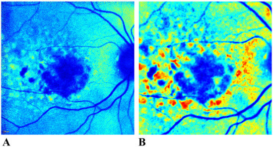
Figure 1.
Application of pseudocoloring (before and after pre-processing the image). If a colormap is applied to a FAF image before pre-processing, as shown in (A), the colormap produces a uniformly colored image which lacks differentiation between the features of interest. Pre-processing before pseudocoloring significantly improves image contrast and enhances feature discrimination (B). FAF: Fundus autofluorescence.
Step 2: Even under carefully designed experimental conditions, artefacts can be a common problem in the image acquisition process. For FAF images, one artefact is the granularity (otherwise known as “salt-and-pepper” noise) in the image. Granularity in this instance does not refer to the mottled appearance of some GA-cases, which would reflect the health and state of the retinal pigment epithelium (RPE, i.e., the spreading and increase in lipofuscin). Rather, granularity is an artefact and therefore needs to be reduced. To minimize image granularity while preserving details in the image, the median filter is very effective [12].
The median filter is a sliding window with a kernel of size placed initially at the top-left corner of the image (i.e., image position [i, j]). The input for the kernel is . The median value of image values within the kernel are [12]. The replacement of the central value in the kernel reduces granularity. For consistency, all images were resized to 768 × 768. There were two original sizes of images: 768 × 768 or 1536 × 1536 pixels with 30° × 30° FOV. The resizing has two essential purposes: (1) it ensures consistency among the cohort (e.g., it provides a single condition for removal of the fuzzy border around FAF images), and (2) image processing is much faster for smaller images, which are still large enough to contain the information needed for discrimination.
Steps 3–5: There are a range of possible colormaps available for pseudocoloring the monochrome image. They include (a) Perceptually Uniform Sequential Colormaps, (b) Sequential Colormaps, (c) Diverging Colormaps, (d) Cyclic Colormaps, (e) Qualitative Colormaps, and (f) Miscellaneous Colormaps. The category of Miscellaneous Colormaps provides the most commonly used color schemes in pseudocoloring. In this group, there are 12 color schemes available: AUTUMN, BONE, JET, WINTER, RAINBOW, OCEAN, SUMMER, SPRING, COOL, HSV, PINK, and HOT [13]. Over the past few years, colormaps such as VIRIDIS have gained popularity and colormaps such as JET (which were once more popular) have receded in popularity [14].
The choice of the colormap is relevant to the required objective of the pseudocoloring operation. In this study, the objective was to enhance the intensity range to improve visual discrimination and to demonstrate the variations in the hyperfluorescent regions which may not normally be visible to the naked eye (but exist in cross-sections of grayscale images). The VIRIDIS colormap only uses three colors, which limits the scope and range of pseudocoloring. Therefore, despite its decline in popularity, the more traditional JET colormap was used in this study owing to its intuitive ease of application, color range and ability to distinguish the different regions of intensity within the hyperfluorescent regions. In a FAF image, the lesion appears as very dark blue, while the retina can range from light blue to green. Hyperfluorescent areas range from yellow to dark red (depending on the degree of hyperfluorescent build-up). The transition from yellow to dark red reflects the level of light or signal intensity within the hyperfluorescent areas. For example, if there is a heavy build-up of lipofuscin in an area, dark red hues would tend to appear in those regions.
The next step in the hyperfluorescent segmentation process is to remove the fuzzy border around FAF images. Due to the image acquisition process, the FAF image has a fuzzy and highly granulated border that contains no significant information about the disease or retina in general. Because of the salt-and-pepper look of the border, the lighter regions may be picked up and misconstrued as hyperfluorescent areas in this process. As a precaution, the fuzzy borders were removed from all FAF images.
Steps 6–8: Following cropping, images are ready for color-based segmentation. However, in order to apply color-based segmentation on the newly created pseudocolored images, conversion to HSV format was necessary (rather than the traditional RGB format). The logic behind the additional conversion of the images to HSV format was because the color ranges representing hyperfluorescent areas were more separable in HSV format than in the RGB format (i.e., we can easily identify the color ranges in HSV). Color ranges representing hyperfluorescent areas were manually identified using the open-source graphic editor GIMP v2.10.4 (https://www.gimp.org/ (accessed on 1 April 2021)). Specifically, the Color Picker tool was used to scroll over the newly colored regions and identify the HSV values for hyperfluorescent areas. These values were used, along with the Python OpenCV inRange() function to extract and create both colored and binarized masks for the hyperfluorescent regions.
Hyperfluorescent regions extracted from FAF images were classified into major transitionary groups (i.e., early to late) in accordance with their changes in intensity and proximity to lesions in FAF images.
2.3. Creation of Foreground Masks for Use in Clustering
The segmentation outputs generated using the automated pseudocoloring methods in the previous section were used to extract the foregrounds (i.e., hyperfluorescent regions) from the backgrounds (i.e., the retina). The objective of this step was to allow the automation method to extract regions of interest from the FAF images so that the FAF image qualities could be used to identify important and clusterable features for hyperfluorescent classification. The following steps were undertaken (Figure 2):
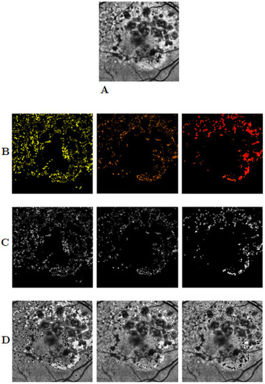
Figure 2.
Separating foreground and background information from FAF images. Image (A) is an example of an original image, while row (B) shows three segmentation outputs using the pseudocoloring segmentation method for hyperfluorescent regions. Row (C) shows the foreground images extracted from the images using the masks in (B). Row (D) shows the background images. FAF: Fundus autofluorescence.
The Foreground Mask Extraction Algorithm (FMEA)
- (1)
- Load the original FAF image together with the binarized segmentation output.
- (2)
- Convert the segmentation output into a grayscale image.
- (3)
- Create a foreground and background threshold mask from the grayscale-converted segmentation output, as follows:
- (a)
- Foreground Mask: Create a foreground mask by thresholding the original mask using the standard Otsu thresholding technique. This converts the image so that the regions of interest become white and the background black. This will later help extract the foreground information only.
- (b)
- Background Mask: Create a background mask by using an inverse Otsu thresholding method, in which now the background pixels are white the background pixels are black. Similarly, this will later be used to help separate the background from the foreground.
- (4)
- Use Bitwise Operations to extract the relevant parts of the image. Using the Bitwise Operation, we specify we want to extract the white portions of our masks (i.e., the newly created Foreground and Background Masks created in Step 3) from the original image. Thus, this method results in two images: an image in which only the foreground information remains (i.e., the hyperfluorescent areas as they appeared in the original FAF images), and a second image with the foreground information removed with only the background information remaining.
The newly extracted foreground images (Figure 2C) were assessed to determine whether clusters exist in the hyperfluorescent regions.
2.4. Image Feature Extraction from Foreground Masks
Features were extracted from the images using the Visual Graphics Group’s (VGG) transfer learning model—the VGG16 [15]. The model is complete with pre-trained weights, see Keras (https://keras.io/ (accessed on 16 April 2021)). The feature extraction process for clustering is described below:
The Feature Extraction Algorithm for Foreground (FEAF)
- (1)
- Load the image and rescale every image to the fixed size of 224 × 224, which is the expected image size for the model.
- (2)
- Convert the image to an array of pixel data.
- (3)
- Expand the shape of the array from a 3D array to a 4D array, with its dimensions listed as [samples, rows, columns, channels].
- (4)
- Use VGG16 pre-processing, converting each image to a BGR color format, and then zero-center each color channel without scaling.
Extract the features from each image using the VGG16 model.
2.5. Cluster Tendency
Testing for cluster tendency is a preliminary step to identify whether the data can form meaningful clusters based on different properties or characteristics [16]. This process involves the application of statistical tests to evaluate the data structure and assesses whether the data are uniformly distributed. A uniform dataset would suggest there is an absence of structure or pattern and any clustering method tested will be unlikely to yield significant results.
To evaluate cluster tendency, the Hopkins statistical test for spatial randomness of a variable can be used [16]. The Hopkins test is denoted as [17]:
where [ refers to a collection of patterns, , in the dimensional space, (i.e., , , where are sampling origins placed at random in space . In the Hopkins statistic, two distances are used: refers to the minimum distance from to its nearest pattern in , and is the distance from a randomly selected pattern in to its nearest neighbor [17]. The null hypothesis for the Hopkins test is that the data contains no clusters and is uniformly distributed. The alternative hypothesis is that the dataset is not uniformly distributed and contains meaningful clusters. The values for the Hopkins test range from 0 to 1. To reject the null hypothesis, the value of would be larger than 0.5 and close to 1 for well-defined clusters. For values less than 0.5, this would suggest the data are regularly spaced and data cannot be clustered. In instances where the space is uniformly distributed, the distances and would be close to each other, whereas if clusters are present, it is anticipated that distances would be substantially larger than .
Note on Software: To execute the Hopkins test in the Python language, the pyclustertend package was used (https://pypi.org/project/pyclustertend/ (accessed on 16 April 2021)). The package uses the formula so that clusterability is interpreted as being a value close to 0. For the pyclustertend package, a high score (i.e., 0.3 and above) suggests that the data cannot be clustered.
2.6. Number of Clusters
The number of clusters tested for statistical significance ranged from k = 2 to k = 12 clusters. The choice of this range was based on the results reported in a pioneering study by Holz et al. (2007) [4]. They suggested four primary patterns of hyperfluorescence, with the diffuse category further divided into an additional five subcategories of patterns, making a total of nine hyperfluorescence patterns (not including the “None” category). For completeness, testing from k = 2 to k = 12 clusters is a reasonable coverage of potential groupings for both lesions and hyperfluorescence, which is also consistent with conjectures in the literature.
2.7. Unsupervised Clustering Methods
A diverse range of clustering algorithms was investigated as part of this analysis. These included Affinity Propagation, Agglomerative Clustering, Balanced Iterative Reducing and Clustering (BIRCH), Density-Based Spatial Clustering of Applications with Noise (DBSCAN), k-Means, Mini-Batch k-Means, and Spectral Clustering. These approaches are described in more detail as follows.
The Affinity Propagation clustering approach identifies samples in the data that are most representative of a cluster, and measures similarities between data samples [18]. Agglomerative Clustering begins by partitioning the data into single nodes and, step by step, merges paired data which are the closest nodes into a new node, until only a single node is left (i.e., the entire dataset) [19]. The BIRCH approach takes large datasets and converts them into more compact, summarised versions that retain as much data distribution information as possible, and uses the data summary in lieu of the original dataset [20]. The DBSCAN approach proposed for spatial databases with noise finds cluster points that are close together within specified distances, and considers points which are far away from the other points as outliers [21]. The k-Means approach relies on the distance between points and calculates cluster centers or centroids, and thus partitions that data around these centroids [22]. The Mini-Batch -Means approach is similar to the more traditional -Means approach. However, rather than using an entire dataset, it uses small batches making this a faster algorithm than its traditional counterpart [23]. The Spectral Clustering approach first constructs a similarity graph of all data points, before using dimensionality reduction and partitioning the data into clusters. Dimensionality reduction refers to the transformation of the data from a high- to low-dimensionality space, with the low-dimensionality space retaining the important properties of the original dataset; this process is also known as spectral embedding [24].
2.8. Visualization of Clusters
Two types of plots were used in the analysis for graphical visualization of clusters: scatter plots and silhouette plots. Scatterplots are used to visualize the placement of datapoints and the clusters using the first and second order statistical features of the datasets showing lesions and hyperfluorescence. Silhouette plots, on the other hand, show how the data are distributed into the respective clusters (i.e., total number of images that go into each cluster), and they also determine whether each assigned cluster exceeds or falls beneath the average silhouette score.
In addition to the above, following the identification of the optimal number of clusters, the original images (i.e., hyperfluorescence segmentation outputs) are automatically labelled according to the specifications of the clustering model. This enables the assessment of the shapes and patterns within each cluster group, and whether the clustering method accurately groups the shapes and patterns, or whether some are mixed. The objective is not just to identify the optimal number of clusters, but to also ensure the classification of the original images into those clusters is correct.
2.9. Data Transformation
Prior to testing the various clustering algorithms, the following transformations were taken to ensure there was no skewness in the data:
- (1)
- Standardization of feature data. This involves removal of the feature mean (average) value and dividing non-constant features by their standard deviation to scale the data, which is equivalent to the statistical z-score [25]. In Python, this is achieved using the StandardScaler() function in the package sklearn (https://scikit-learn.org/stable/ (accessed on 20 April 2021)).
- (2)
- Reducing the complexity of the data using Principal Component Analysis (PCA), which transforms the collections of correlated features extracted from the images and condenses them into smaller, uncorrelated variables named principal components [26]. This is achieved using the Python sklearn function PCA().
2.10. Cluster Evaluation Metrics
There are different metrics which can be used for evaluation of meaningful clusters. The choice is contingent on whether we use an intrinsic (i.e., internal) cluster quality measure or an extrinsic (i.e., external) measure. The analysis presented here is for unsupervised clustering methods where there is no prior knowledge (unlike supervised learning). Therefore, to assess the quality of the clustering method, we adopt an intrinsic approach and evaluate the properties of the data itself. For this analysis, internal validation measures were used, such as the Silhouette Coefficient (SC), the Davies–Bouldin Index (DBI), and the Calinski–Harabasz Index (CHI).
The SC is a proximity measure, assessing both the compactness of clusters as well the separation of clusters from one another. It relies on two features: the partitions obtained from the clustering method, and the proximities of all datapoints. It uses these two features to assess (1) how close each data point is to data points within its own cluster, and (2) how distant each data point is from data points in other clusters. The SC formula is denoted as:
where is any object in the data (i.e., image features), is the average dissimilarity of to all other objects of the cluster , is the average dissimilarity of to all objects of cluster , and is smallest number of datapoints which for all clusters where (i.e., = minimum [27]. The values for the SC range from −1 to +1. Negative values indicate the assignment of incorrect clusters, while values around 0 may suggest borderline results, and finally positive values indicate good clusters, particularly values which are 0.5 and higher. In fact, the higher the value, the more we can validate that good clustering has been identified (i.e., data points are well matched to their cluster and poorly matched to neighboring clusters).
The DBI is a cluster separation measure and possesses the following qualities: (1) it can be applied to hierarchical datasets, (2) it is computationally feasible for even large datasets, and (3) can yield meaningful results for data of arbitrary dimensionality [28]. The objective of DBI is to identify whether clusters are well-spaced from each other, and whether each cluster is very dense and likely to be a good cluster. It calculates the ratio of the sum of the average distances between two clusters and between cluster centers [29]. The formula for the DBI is:
where is the number of clusters, is the average distance of all points in cluster , is the average distance of all points in cluster , and and are the cluster centroids for clusters and , respectively. Conversely to the SC, the rule of thumb for the DBI is that the smaller the value the better the clustering method. The minimum score for this index is 0, and thus ideally anything that is close to the 0 mark is indicative of a good clustering method.
The CHI, also known as the Variance Ratio Criterion, evaluates the ‘tightness’ of within clusters (i.e., inter-cluster dispersion) as well as between clusters (i.e., between-cluster dispersion) [29,30]. The CHI is defined as [29]:
where is the number of corresponding clusters, and is the inter-cluster divergence, and is the intra-cluster divergence, and is the total number of samples. A smaller indicates a good inter-cluster dispersion, while a high indicates a good between-cluster dispersion. The larger a CHI ratio is the better the clustering effect [29].
3. Results
3.1. Data Summary
A total of 702 FAF images from 51 patients with GA secondary to AMD were collected in this study [10]. For this subanalysis, 524 of the original 702 FAF images were found to have all stages of hyperfluorescence identified in the automation phase. The cohort of images and patients were quite large and diverse as compared to others in GA-AI segmentation studies [9]. The cohort consisted of 99 eyes, 49 left eyes (49.5%) and 50 right eyes (50.5%). A total of 359 images were for the left eye and 343 images were for the right eye. The cohort consisted of 38 female (74.5%) and 13 males (25.5%) with an average age of 76.7 ± 8.9 years. Total follow-up time was 61.5 ± 25.3 months. The intraclass correlation coefficient for consistency between the two graders was 0.9855 (95% CI: 0.9298, 0.9971), showing close agreement between the graders.
3.2. Hyperfluorescence Segmentation
Using the JET colormap, the following regions were highlighted and labelled accordingly:
- Regular retinal regions: These areas are typically represented by varying levels of blue, which represent the general retinal regions, including ocular features such as the optic disc and blood vessels.
- Early-stage hyperfluorescent development: These regions have a yellowish tinge and are early signs of degeneration (i.e., precursor to more intense hyperfluorescent development typically seen in FAF images).
- Intermediate-stage hyperfluorescent development: The orange regions are classified as intermediate, given that in FAF they appear in border-like formation around the brightest regions of hyperfluorescent areas.
- Late-stage hyperfluorescent development: The hyperfluorescent regions of greatest intensity are classified as late stage. These are the areas thought to be precursors to lesion development.
These regions are clearly highlighted in Figure 3. To extract the different hyperfluorescent stages and regions from the pseudocolored images, the following values were identified (using GIMP software) and were used in the extraction of varying hyperfluorescent regions:
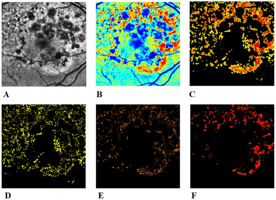
Figure 3.
Hyperfluorescent segmentation using pseudocoloring. (A) Pre-processed image. (B) Application of the JET colormap, which shows different stages of hyperfluorescence development. (C) Extraction all stages combined. (D) Early-stage hyperfluorescence development. (E) Intermediate-stage hyperfluorescence development. (F) Late-stage hyperfluorescence development. This late stage appears to be the precursor to lesion formation, as intensity levels (i.e., build-up of lipofuscin) reach a peak before retinal cellular death occurs.
- Early stage: Minimum HSV values: [25, 62, 0]. Maximum HSV values: [35, 255, 255].
- Intermediate stage: Minimum HSV values: [12, 255, 255]. Maximum HSV values: [17, 255, 255].
- Late stage: Minimum HSV values: [0, 62, 0]. Maximum HSV values: [10, 255, 255].
The values were extracted as ranges to ensure extraction of the lower and upper limits of the colors in the pseudocolored images. While we have identified several hyperfluorescent development stages, the one with the greatest importance to lesion formation is the late-stage (i.e., red) regions, given that the dark red regions represent high-intensity areas (i.e., strong lipofuscin build-up) and are expected to progress into lesion areas due to retinal cellular death.
Qualitative assessments were utilized as no ground truths were available for running standard segmentation metrics, such as the Dice similarity coefficient. Visual assessments for hyperfluorescent segmentation illustrated good segmentation performance. The hyperfluorescent segmentation also takes only 5–6 s per image to process the data.
3.3. Cluster Tendency
Cluster tendency was evaluated at all three stages of hyperfluorescence (Table 1). The cluster tendency was 0.1010 for early-stage hyperfluorescence, 0.0899 for intermediate-stage hyperfluorescence, and 0.0895 for late-stage hyperfluorescence. These results indicate that there are cluster patterns within the data that can be extrapolated.

Table 1.
Cluster tendency for GA features, including lesions and early-, intermediate-, late-stage hyperfluorescent areas.
3.4. Evaluation of Unsupervised Clustering Methods
The Affinity Propagation algorithm was eliminated from the process early in this study. While some clustering algorithms, such as -Means and Agglomerative algorithms, allow the user to specify and explore the impact of changing the number of clusters, Affinity Propagation does not require the manual input of ‘cluster number’. Rather, it requires appropriate modification of its parameters and then identifies the most suitable clusters through these parameters.
For Affinity Propagation, the two important parameters are denoted as preference (controls how many clusters are found) and damping (a numerical stabilizer that can be regarded as the learning rate). Several values of preference and damping were evaluated. However, despite many attempts at tweaking the parameters, the number of clusters produced from Affinity Propagation were always extremely large. The lowest number of clusters identified was = 92 clusters for lesions, = 95 clusters for early-stage hyperfluorescence, = 102 clusters for intermediate-stage hyperfluorescence, and = 119 clusters for late-stage hyperfluorescence. These values were achieved by using a damping factor of 0.9, and the preference option excluded.
Another method which does not require the input of a potential cluster number is DBSCAN. DBSCAN also requires the modification of appropriate parameters to optimize and identify the most appropriate clusters for a dataset. The most prominent parameter for DBSCAN is referred to as epsilon. Epsilon is defined as the maximum distance between two datapoints. Rahmah and Sitanggang (2016) proposed an automated method of tuning epsilon [31]. The processing involves finding the shortest distance between each data point and its nearest neighbor, then sorting these distances in ascending order, and plotting the results on a curve. The point at which maximum curvature takes place on a curve is where the optimal epsilon value for the dataset can be found. Optimal epsilons were calculated for all hyperfluorescent regions (Table 2). For early-hyperfluorescence, an epsilon value of 10 was found to be the most appropriate. Optimal epsilon value for intermediate-stage hyperfluorescence was 31 and 16 for late-stage hyperfluorescence.
Table 2.
Results for DBSCAN.
Despite the automated method of selecting optimal epsilon values for each hyperfluorescence region, there was an inconsistency in the results. While some SCs were good (i.e., intermediate-stage hyperfluorescence had a SC of 0.829), the DBI and CHI were not ideal (i.e., DBIs were larger than expected, and CHIs smaller). As a result, the DBSCAN was ruled out as an appropriate clustering technique.
Another method that was ruled out early in this study was Spectral Clustering. Unlike DBSCAN and Affinity Propagation, the user can specify different cluster numbers and determine the quality of the output. Using Spectral Clustering, typically 2–3 clusters would be identified at most (Table 3). However, any attempts at looking at clusters larger than 2–3 would yield warnings and produce identical results, irrespective of the cluster being tested. There could be several reasons for this, namely: (1) Spectral Clustering is sensitive to change in the similarity map, and (2) Spectral Clustering works well with balanced datasets (i.e., datasets with even occurrences of different classification categories), and falter if there are large differences between the datapoints within the clusters [32].
Table 3.
Results for spectral clustering.
Optimal cluster analyses were pursued using the remaining clustering methods: k-Means (Table 4), Agglomerative (Table 5), BIRCH (Table 6), and Mini-Batch k-Means (Table 7). To select the most appropriate number of clusters within each analysis, the following process was followed:
Table 4.
Results for k-Means clustering.
Table 5.
Results for Agglomerative clustering.
Table 6.
Results for BIRCH clustering.
Table 7.
Results for Mini-Batch k-Means clustering.
- (1)
- The top two highest SC scores were noted.
- (2)
- From the top two SC scores, the cluster typically with the lowest DBI coupled with the highest CHI was selected.
- (3)
- In addition to the scores, the scatter plots were also evaluated to see how clearly defined the clusters were, and whether visually the cluster numbers selected made sense.
Additionally, a choice had to be made regarding the most appropriate algorithm for the data. The top two contender algorithms were k-Means (Table 4) and Agglomerative (Table 5), which generally produced more favourable results as compared to BIRCH (Table 6) and Mini-Batch k-Means (Table 7). Given the similarity in quantitative results and scatter plots, an additional approach was taken to discern one method from the other: to visually assess how the shapes and patterns of lesions and hyperfluorescence areas were being categorized (i.e., to see how the 524 images were being divided into their respective clusters), and if the categorization looked consistent. The k-Means produced more consistent categorization (Figure 4, Figure 5, Figure 6 and Figure 7), as patterns and shapes of hyperfluorescent areas within the clusters assigned seemed consistent, whereas Agglomerative had some inconsistencies (i.e., some cluster groups had mixed shapes that did not seem to belong together). Therefore, the k-Means clustering method was chosen as the most appropriate for this dataset. The most appropriate number of clusters per hyperfluorescent region is shown in Table 8.
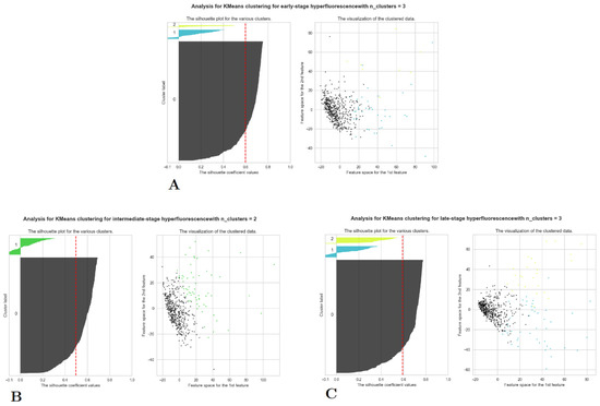
Figure 4.
Scatter and silhouette plots for lesions and hyperfluorescent regions using k-Means clustering. (A) early-stage hyperfluorescence, (B) intermediate-stage hyperfluorescence, and (C) late-stage hyperfluorescence.
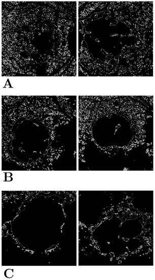
Figure 5.
Early-stage hyperfluorescence shape and pattern clustering using k-Means. (A) Cluster group 1, (B) cluster group 2, and (C) cluster group 3. There appears to be three groups of early-stage hyperfluorescence: one in which early-stage covers the majority of the retina (i.e., early-stage hyperfluorescence complete coverage [EHCC]) (A), another with partial coverage (i.e., early-stage hyperfluorescence partial coverage [EHPaC]) (B), and finally, one that simply surrounds the proximity of the lesions (i.e., early-stage hyperfluorescence proximal coverage [EHPrC]) (C).
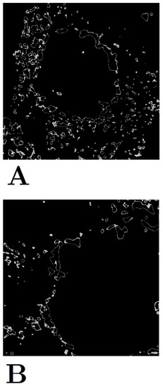
Figure 6.
Intermediate-stage hyperfluorescence shape and pattern clustering using k-Means. (A) Cluster group 1 and (B) Cluster group 2. Unlike the early- and late-stage hyperfluorescence groups, the intermediate-stage grouping is not as prominent.
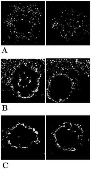
Figure 7.
Late-stage hyperfluorescence shape and pattern clustering using k-Means. (A) Cluster group 1, (B) cluster group 2, and (C) cluster group 3. There appears to be three groups of late-stage hyperfluorescence: one in which there is a small scatter of hyperfluorescence regions (i.e., late-stage hyperfluorescence droplet scatter [LHDS])) (A), another combines the scatter with a halo ring around the lesion (i.e., late-stage hyperfluorescence halo scatter [LHHS] (B), and finally, one that is simply a halo around the lesions (i.e., late-stage hyperfluorescence halo [LHH]) (C).
Table 8.
Optimal number of clusters.
Based on the visual outcomes of the clusters (i.e., the appearance of shapes and patterns within each clustered group), new names have been assigned to hyperfluorescence categories (Table 9).
Table 9.
Suggested new categorization of GA features.
4. Discussion
The automation of hyperfluorescence segmentation is described using a pseudocoloring method employing the application of the JET colormap to capture hyperfluorescent intensity changes. Regions of hyperfluorescence are difficult to annotate due to their spatial distribution, frequency and poor visibility. The pseudocoloring process aided in segmentation of hyperfluorescence flagged in FAF images and also revealed additional areas previously missed. This technique can be used to expedite clinical and research investigations into hyperfluorescence and its association with GA progression. In the segmentation process, three transitionary stages of hyperfluorescence were identified based both on the intensity changes in lipofuscin build-up as well as the proximity of these stages to the GA lesions boundaries. These new transition stages have been labelled as early-, intermediate-, and late-stage hyperfluorescence regions.
The clustering of hyperfluorescence areas is also described in this study, with the newly identified transitionary stages assessed for further analysis. Publications to date have evaluated the categorization of hyperfluorescence patterns, with categories including none, focal, banded, diffuse, and patchy (as described in Holz et al.) [4]. The diffuse category is further divisible into reticular, branching, fine granular, trickling, and GPS. However, the repeatability and reproducibility of these categories has varied, with associations with these patterns and their influence on GA progression not always showing statistical significance. Furthermore, while Fleckenstein et al. [33]. showed an illustrative example of how different lesion types correlated with different progression rates, it was an indirect implication—lesion categorization was not fully explored as hyperfluorescence categorization. Therefore, in this study, it was hypothesized that unsupervised clustering algorithms could be used to distinguish the different categories of hyperfluorescence shapes and patterns, and these new cluster patterns could be associated with future GA progression.
The clustering algorithms which were tested included k-Means, Agglomerative, Affinity Propagation, BIRCH, DBSCAN, Mini-Batch k-Means, and Spectral Clustering. A combination of metrics (i.e., SC, DBI, and CHI) were used alongside visualization techniques to determine (1) the optimal number of clusters, and (2) the best unsupervised clustering algorithm for GA data. The number of clusters of interest ranged from k = 2 to k = 12. The choice of this range is in-line with current studies which suggest that regions of hyperfluorescence can be divided into five main categories (i.e., none, focal, diffuse, banded and patchy), and a further five subcategories. Affinity Propagation, DBSCAN, and Spectral Clustering were eliminated early in the evaluation process. Parameter sensitive Affinity Propagation resulted in very large cluster numbers (i.e., over 90 clusters for lesion and hyperfluorescent data). The other parameter-sensitive algorithm, DBSCAN, produced good SC scores, however, less than ideal DB and CHI scores, which resulted in its early elimination. Spectral Clustering was also removed, given that it produced identical results for all clusters, typically after k = 2. The repetitiveness of results with the use of Spectral Clustering can have many factors, but one which may be most probable for this dataset is that the dataset is not balanced (i.e., there is not an equality of cases for each cluster).
Among the remaining algorithms, k-Mean and Agglomerative clustering were the main contenders. They both had favourable SC, DBI, and CHI outcomes, and showed more distinguishable and separable clusters in the scatter plots. However, when it came to seeing how each image was clustered, the shapes and patterns within each cluster as produced by k-Means was much more consistent than Agglomerative, with the latter having the tendency to mix-in different shapes and patterns into one cluster group. As a result, the k-Means, a simple partitioning cluster method, was chosen as the best unsupervised clustering method (in combination with pre-processing techniques, such as scaling and PCA) for GA feature data.
The optimal number of clusters for early-stage hyperfluorescence areas was k = 3, with a SC of 0.597, a DBI of 0.915, and a CHI of 186.99. For intermediate-stage hyperfluorescence, an optimal cluster of k = 2 was identified, with a SC of 0.496, a DBI of 1.282, and a CHI of 144.92. Finally, for the late-stage hyperfluorescence, optimal cluster of k = 3 was identified, with an SC of 0.593, a DBI of 1.013, and a CHI of 217.325. Amongst these results, the one with intermediate-stage hyperfluorescence results present the greatest uncertainty, given it has the lowest value of SC. Scatter plots of lesions demonstrated extremely discernible cluster of three in the scatter plots. While the scatter plots for early-, intermediate and late-stage hyperfluorescence also showed good clustering visually, these clusters were not as distinguishable as those of the lesions cluster plot.
The three categories of early-stage hyperfluorescence clustering are presented in Figure 5. The cluster groups appear to represent the level of coverage of early-stage hyperfluorescence across the retina. The first pattern involves the coverage of the entire retina, while the second pattern covers the retina partially. Finally, the third pattern covers the perimeter of the lesion. These patterns have been named as (1) early-stage hyperfluorescence complete coverage (EHCC), (2) early-stage hyperfluorescence partial coverage (EHPaC), and (3) early-stage hyperfluorescence proximal coverage (EHPrC).
The two clusters of intermediate-stage hyperfluorescence are not as clear-cut in their patterns as the lesions and early-stage hyperfluorescence (Figure 6), thus explaining the lower SC scores. No names have been given to these yet, given that intermediate-stage clustering may simply represent a transitional stage between the early and late stages of hyperfluorescence.
Finally, the three stages of late-stage hyperfluorescence clustering are presented in Figure 7. The first category of late-stage patterns shows a small, circle scattering of hyperfluorescence droplets, while the second category combines these droplet scatters with a halo surrounding the lesion. Lastly, the third pattern shows a very distinct and dense halo directly surrounding the lesion, that most likely illustrates peak lipofuscin intensity which precedes lesion formation. These regions have been therefore named as (1) late-stage hyperfluorescence droplet scatter (LHDS), (2) late-stage hyperfluorescence halo scatter (LHHS), and (3) late-stage hyperfluorescence halo (LHH). All newly identified GA feature categories can be found in Table 9.
One of the potential limitations of cluster analysis is the requirement for parameter tuning for some clustering methods, such as Affinity Propagation and DBSCAN. Even though attempts were made to automate the selection of the epsilon parameters for DBSCAN, the results can change given their sensitivity to parameter changes. Proper settings can only be established by trial-and-error, and the analysis presented here was no exception [28]. From establishing the most appropriate data transformations, to testing the different algorithms, and the selection of parameters, there is a still a component of human error in unsupervised clustering that needs to be addressed. Another potential limitation exists with the cases available in this cohort. The clustering was based on the shapes and patterns of the data in the trial. However, this dataset may not be representative of all GA cases and future research could investigate further applications to new data sets.
Future research could replicate these findings in larger and more diverse cohorts, further establishing the validity of the hyperfluorescent classifications identified in this study. Furthermore, the application of these hyperfluorescent classes in disease progression modelling can be used to validate the influence of the classification on predictive capabilities. In line with previous research, establishing correlations between the identified hyperfluorescent categories and disease progression rates could shed additional light on the significance of hyperfluorescence monitoring in GA progression. Additionally, epidemiological investigations might illuminate how the predictive performance of hyperfluorescent patterns vary across different cohorts. Complementing such research, genetic association studies could provide valuable insights, revealing inheritable patterns that might explain the differing appearances and spatial distributions of hyperfluorescent regions within the retina.
These classifications could lead to the development of more robust prediction models that could be used in a real-time clinical setting to predict progression severity and rate. The developed models, along with their incorporated features, could foster a personalized approach to diagnosis and patient care, leading to the potential formulation of tailored therapies. In a clinical setting, healthcare providers could leverage hyperfluorescence readings to forecast patient prognosis right from the baseline, specifically identifying those at higher risk of rapid progression. This practice could empower clinicians to better manage patients’ well-being, leading to timely and effective interventions.
5. Conclusions
In the past, progression of GA in late-stage AMD was monitored over time using time-series images showing lesions and their growth trajectories based on increasing geometrical areas of hypofluorescence. It was observed by some researchers that further information on prediction of GA growth rates may be derived from the shape and structure of the boundaries surrounding the GA lesions, which appear in FAF images as bright areas of hyperfluorescence. In a seminal study, Holz and co-workers proposed a taxonomy of hyperfluorescence shapes and patterns that may appear in an image and could be associated with different growth rates of GA [4].
The proposed taxonomy suggested by Holz et al. was based on subjective descriptions of the spatial appearance and geometry of patterns of hyperfluorescence. The number of categories chosen was also subjective. In the study reported here, digital image processing and unsupervised learning were used for clustering the pattern types into a finite number of categories that could be associated with different GA growth rates. An important contribution of the analysis reported in this paper is that it reduces the number of categories and provides a taxonomy that is objective and not subjective. A noteworthy feature of the approach used is the automation of the operation of segmentation using pseudocoloring techniques.
The analysis required digital image processing to transform (normalise) the data by contrast limited adaptive histogram equalization followed by the application of clustering methods, such as k-Means and Agglomerative Clustering. Following exhaustive analysis of unsupervised clustering methods, based on evaluation against a range of performance metrics, the most effective method used the k-Means algorithm. The optimum number of clusters were identified (see Table 8). The categorizations described here (see Table 9) can be used in guiding future studies of GA growth rates.
Author Contributions
Conceptualization, J.A. and K.B.; methodology, J.A. and K.B.; validation, J.A.; formal analysis, J.A.; investigation, J.A. and K.B.; writing—original draft preparation, J.A. and K.B.; writing—review and editing, J.A. and K.B.; visualization, J.A.; supervision, K.B. All authors have read and agreed to the published version of the manuscript.
Funding
This research received no external funding.
Institutional Review Board Statement
This study was conducted in accordance with the Declaration of Helsinki and approved by the Institutional Review Board (or Ethics Committee) of the Royal Victorian Eye and Ear Hospital (HREC: Project No. 95/283H/15).
Informed Consent Statement
Informed consent was obtained from all subjects involved in this study.
Data Availability Statement
Not applicable.
Conflicts of Interest
The authors declare no conflict of interest.
References
- Yung, M.; Klufas, M.A.; Sarraf, D. Clinical applications of fundus autofluorescence in retinal disease. Int. J. Retin. Vitr. 2016, 2, 12. [Google Scholar] [CrossRef] [PubMed]
- Mata, N.L.; Lichter, J.B.; Vogel, R.; Han, Y.; Bui, T.V.; Singerman, L.J. Investigation of oral fenretinide for treatment of geographic atrophy in age-related macular degeneration. Retina 2013, 33, 498–507. [Google Scholar] [CrossRef] [PubMed]
- Holz, F.G.; Spaide, R.F. Medical Retina [Electronic Resource]; Springer: Berlin/Heidelberg, Germany; New York, NY, USA, 2007. [Google Scholar]
- Holz, F.G.; Bindewald-Wittich, A.; Fleckenstein, M.; Dreyhaupt, J.; Scholl, H.P.; Schmitz-Valckenberg, S.; Group, F.A.-S. Progression of geographic atrophy and impact of fundus autofluorescence patterns in age-related macular degeneration. Am. J. Ophthalmol. 2007, 143, 463–472. [Google Scholar] [CrossRef] [PubMed]
- Jeong, Y.J.; Hong, I.H.; Chung, J.K.; Kim, K.L.; Kim, H.K.; Park, S.P. Predictors for the progression of geographic atrophy in patients with age-related macular degeneration: Fundus autofluorescence study with modified fundus camera. Eye 2014, 28, 209–218. [Google Scholar] [CrossRef]
- Batioglu, F.; Gedik Oguz, Y.; Demirel, S.; Ozmert, E. Geographic atrophy progression in eyes with age-related macular degeneration: Role of fundus autofluorescence patterns, fellow eye and baseline atrophy area. Ophthalmic Res. 2014, 52, 53–59. [Google Scholar] [CrossRef]
- Biarnes, M.; Arias, L.; Alonso, J.; Garcia, M.; Hijano, M.; Rodriguez, A.; Serrano, A.; Badal, J.; Muhtaseb, H.; Verdaguer, P.; et al. Increased Fundus Autofluorescence and Progression of Geographic Atrophy Secondary to Age-Related Macular Degeneration: The GAIN Study. Am. J. Ophthalmol. 2015, 160, 345–353. [Google Scholar] [CrossRef]
- Arslan, J.; Benke, K.K. Progression of Geographic Atrophy: Epistemic Uncertainties Affecting Mathematical Models and Machine Learning. Transl. Vis. Sci. Technol. 2021, 10, 3. [Google Scholar] [CrossRef]
- Arslan, J.; Samarasinghe, G.; Benke, K.K.; Sowmya, A.; Wu, Z.; Guymer, R.H.; Baird, P.N. Artificial Intelligence Algorithms for Analysis of Geographic Atrophy: A Review and Evaluation. Transl. Vis. Sci. Technol. 2020, 9, 57. [Google Scholar] [CrossRef]
- Arslan, J.; Samarasinghe, G.; Sowmya, A.; Benke, K.K.; Hodgson, L.A.B.; Guymer, R.H.; Baird, P.N. Deep Learning Applied to Automated Segmentation of Geographic Atrophy in Fundus Autofluorescence Images. Transl. Vis. Sci. Technol. 2021, 10, 2. [Google Scholar] [CrossRef]
- Zhou, L.; Hansen, C.D. A Survey of Colormaps in Visualization. IEEE Trans. Vis. Comput. Graph. 2016, 22, 2051–2069. [Google Scholar] [CrossRef]
- Sun, T.; Neuvo, Y. Detail-preserving median based filters in image processing. Pattern Recognit. Lett. 1994, 15, 341–347. [Google Scholar] [CrossRef]
- Matplotlib. Choosing Colormaps in Matplotlib. Available online: https://matplotlib.org/stable/tutorials/colors/colormaps.html (accessed on 1 April 2021).
- Nuñez, J.R.; Anderton, C.R.; Renslow, R.S. Optimizing colormaps with consideration for color vision deficiency to enable accurate interpretation of scientific data. PLoS ONE 2018, 13, e0199239. [Google Scholar] [CrossRef]
- Simonyan, K.; Zisserman, A. Very Deep Convolutional Networks for Large-Scale Image Recognition. arXiv 2015, arXiv:1409.1556. [Google Scholar]
- Vandeginste, B.G.M.; Massart, D.L.; Buydens, L.M.C.; De Jong, S.; Lewi, P.J.; Smeyers-Verbeke, J. Chapter 30—Cluster analysis. In Data Handling in Science and Technology; Vandeginste, B.G.M., Massart, D.L., Buydens, L.M.C., De Jong, S., Lewi, P.J., Smeyers-Verbeke, J., Eds.; Elsevier: Amsterdam, The Netherlands, 1998; Volume 20, pp. 57–86. [Google Scholar]
- Banerjee, A.; Dave, R.N. Validating clusters using the Hopkins statistic. In Proceedings of the 2004 IEEE International Conference on Fuzzy Systems (IEEE Cat. No.04CH37542), Budapest, Hungary, 25–29 July 2004; Volume 141, pp. 149–153. [Google Scholar]
- Bodenhofer, U.; Kothmeier, A.; Hochreiter, S. APCluster: An R package for affinity propagation clustering. Bioinformatics 2011, 27, 2463–2464. [Google Scholar] [CrossRef] [PubMed]
- Müllner, D. Modern hierarchical, agglomerative clustering algorithms. arXiv 2011, arXiv:1109.2378. [Google Scholar]
- Zhang, T.; Ramakrishnan, R.; Livny, M. BIRCH: A New Data Clustering Algorithm and Its Applications. Data Min. Knowl. Discov. 1997, 1, 141–182. [Google Scholar] [CrossRef]
- Mahesh Kumar, K.; Rama Mohan Reddy, A. A fast DBSCAN clustering algorithm by accelerating neighbor searching using Groups method. Pattern Recognit. 2016, 58, 39–48. [Google Scholar] [CrossRef]
- Likas, A.; Vlassis, N.; Verbeek, J.J. The global k-means clustering algorithm. Pattern Recognit. 2003, 36, 451–461. [Google Scholar] [CrossRef]
- Sculley, D. Web-scale k-means clustering. In Proceedings of the 19th International Conference on World Wide Web, Raleigh, NC, USA, 26–30 April 2010; pp. 1177–1178. [Google Scholar]
- Aggarwal, C.C.; Reddy, C.K. Data Clustering, 1st ed.; Chapman and Hall/CRC: Boca Raton, FL, USA, 2014. [Google Scholar]
- Stoddard, A.M. Standardization of Measures Prior to Cluster Analysis. Biometrics 1979, 35, 765–773. [Google Scholar] [CrossRef]
- Maadooliat, M.; Huang, J.Z.; Hu, J. Integrating Data Transformation in Principal Components Analysis. J. Comput. Graph Stat. 2015, 24, 84–103. [Google Scholar] [CrossRef]
- Rousseeuw, P.J. Silhouettes: A graphical aid to the interpretation and validation of cluster analysis. J. Comput. Appl. Math. 1987, 20, 53–65. [Google Scholar] [CrossRef]
- Davies, D.L.; Bouldin, D.W. A Cluster Separation Measure. IEEE Trans. Pattern Anal. Mach. Intell. 1979, PAMI-1, 224–227. [Google Scholar] [CrossRef]
- Wang, X.; Xu, Y. An improved index for clustering validation based on Silhouette index and Calinski-Harabasz index. IOP Conf. Ser. Mater. Sci. Eng. 2019, 569, 052024. [Google Scholar] [CrossRef]
- Caliński, T.; Harabasz, J. A dendrite method for cluster analysis. Commun. Stat. 1974, 3, 1–27. [Google Scholar] [CrossRef]
- Rahmah, N.; Sitanggang, I.S. Determination of Optimal Epsilon (Eps) Value on DBSCAN Algorithm to Clustering Data on Peatland Hotspots in Sumatra. IOP Conf. Ser. Earth Environ. Sci. 2016, 31, 012012. [Google Scholar] [CrossRef]
- Nadler, B.; Galun, M. Fundamental Limitations of Spectral Clustering. In Proceedings of the Advances in Neural Information Processing Systems 19 (NIPS 2006), Vancouver, BC, Canada, 4–7 December 2006. [Google Scholar]
- Fleckenstein, M.; Mitchell, P.; Freund, K.B.; Sadda, S.; Holz, F.G.; Brittain, C.; Henry, E.C.; Ferrara, D. The Progression of Geographic Atrophy Secondary to Age-Related Macular Degeneration. Ophthalmology 2018, 125, 369–390. [Google Scholar] [CrossRef] [PubMed]


Disclaimer/Publisher’s Note: The statements, opinions and data contained in all publications are solely those of the individual author(s) and contributor(s) and not of MDPI and/or the editor(s). MDPI and/or the editor(s) disclaim responsibility for any injury to people or property resulting from any ideas, methods, instructions or products referred to in the content. |
© 2023 by the authors. Licensee MDPI, Basel, Switzerland. This article is an open access article distributed under the terms and conditions of the Creative Commons Attribution (CC BY) license (https://creativecommons.org/licenses/by/4.0/).