Article

Comparison of Imputation Methods for Activated Sludge Data: A Case Study on Imputing Missing Data


School of Energy, Geoscience, Infrastructure and Society, Heriot-Watt University, Dubai Campus, Dubai Knowledge Park, Dubai P.O. Box 501745, United Arab Emirates
*
Author to whom correspondence should be addressed.
Waste 2026, 4(2), 17; https://doi.org/10.3390/waste4020017
Submission received: 28 January 2026 / Revised: 30 April 2026 / Accepted: 20 May 2026 / Published: 28 May 2026

Abstract

The activated sludge process is pivotal in wastewater treatment, with ongoing research into its process control methods. Modeling treatment plants aids in analyzing relationships among variables, supporting fault detection and operational decision-making. However, datasets from real-world treatment plants often contain outliers and missing values due to sensor faults, maintenance activities, and operational disruptions, making outlier handling and data imputation essential for reliable modeling. Existing studies on data imputation for activated sludge systems are often based on synthetic or short datasets, limited method comparisons, or inconsistent evaluation metrics, which reduces their applicability to full-scale operational settings. This study addresses these limitations by presenting a comprehensive, head-to-head comparison of Kohonen Self-Organising Maps (KSOM) with widely used multiple imputation and tree-based methods, namely Amelia II, MICE, missForest, and missRanger. The methods are applied to a real-world multivariate dataset comprising 19 process variables collected over 8.5 years from a full-scale activated sludge treatment plant, containing 39% overall missing data with highly uneven missingness across variables. A validation framework based on held-out observation data is used, and performance is assessed using complementary metrics, including the coefficient of determination (R2), average absolute error (AAE), relative average absolute error (RAAE), mean squared error (MSE), and root mean squared error (RMSE). Results show that KSOM consistently outperforms the competing methods across most variables and evaluation metrics. KSOM achieves near-perfect R2 values (≈1) for many process variables, with lower absolute and relative errors, even for variables with very high (>70%) and irregular missingness. These findings highlight KSOM’s robustness in capturing multivariate relationships and cluster structure in complex, operational WWTP data.

1. Introduction

Clean water is crucial for survival, and using the available limited water resources efficiently and safely is vital. The United Nations’ Sustainable Development Goals (SDGs) aim to achieve several water and wastewater infrastructure goals by 2030. One of these goals is to ensure that everyone has access to clean water and sanitation while sustainably managing water resources. This includes wastewater treatment and safe reuse [1,2,3,4]. Wastewater treatment plants (WWTPs) play a critical role in achieving these targets, typically using combinations of primary, secondary and/or tertiary treatments. Among these, secondary biological treatment based on the Activated Sludge Process (ASP) is the most widely used, due to its efficiency, flexibility, and suitability for large-scale operation [5,6,7].
Reliable, high-quality process data obtained from online sensors, laboratory measurements and operational logs is essential for modelling, monitoring and control of ASP systems [7,8]. Such data is useful for fault detection, process optimization, and regulatory compliance [9,10,11]. However, real-world datasets collected from full-scale WWTPs frequently contain outliers and large, unevenly distributed gaps caused by sensor faults, maintenance activities, communication failures and operational disruptions. These data quality issues can significantly affect model accuracy, introduce bias, and hinder operational decision-making [12,13]. This makes effective data preprocessing and imputation essential for data-driven analysis [14,15,16].
Research on WWTP data and modelling has progressed along two complementary directions. Mechanistic approaches based on activated sludge models (ASM1, ASM2, ASM3) provide valuable process insight and are widely used for design and control. However, they require extensive parameterization and can be difficult to apply to long-term, full-scale datasets. Data-driven and machine learning (ML) approaches have gained increasing attention over the last decade, enabling the analysis of complex WWTP processes without the need for mechanistic equations. Reviews and recent studies highlight the potential of ML for monitoring, forecasting and adaptive control. However, model performance is highly sensitive to data quality, particularly the presence and structure of missing values.
To address missing data, a broad range of imputation techniques have been developed. Simple single-imputation approaches (e.g., mean or median substitution) are easy to implement but often distort variance and correlations in multivariate process data. Multiple imputation methods, such as Multivariate Imputation by Chained Equations (MICE) and Amelia II, explicitly account for uncertainty and inter-variable dependence and are commonly applied to complex datasets [17,18]. Tree-based iterative methods, including MissForest and MissRanger, analyze nonlinear relationships and interactions using random forests and have demonstrated strong performance across environmental and industrial datasets [19,20,21,22]. Unsupervised clustering approaches, particularly Kohonen Self-Organising Maps (KSOM), infer missing values by analyzing patterns within the data, and have shown promise in applications involving strongly correlated process variables.
Several studies have explored these approaches in the context of wastewater data. Chmielowski et al. [23] compared support vector machines and k-nearest neighbours for imputing water quality indicators, showing improved performance for SVMs but without accounting for inter-variable correlations. Kim et al. [24] conducted a broader comparison of imputation methods for water quality data, highlighting the suitability of Amelia II for time-series applications and the advantages of random-forest-based methods for continuous sensor data. Rustum and Adeloye [25] applied KSOM to activated sludge data from the Seafield WWTP, reporting strong predictive performance for several variables and suggesting that KSOM is relatively insensitive to the number of missing values. Nijim and Rustum [26] further compared KSOM and MICE for dissolved oxygen imputation, concluding that KSOM performs well at low to moderate missingness, whereas all methods deteriorate as missingness exceeds 40%. Tree-based methods such as MissForest and MissRanger have also been shown to outperform simpler approaches in mixed-type datasets, but at the cost of increased computational demand, particularly for large datasets with extensive missingness [19,20,21,22].
Despite these advances, important gaps remain. Most existing studies are limited to synthetic datasets, short monitoring periods, or single variables or focus on a narrow selection of methods, offering little insight into performance under realistic, full-scale operating conditions. Many studies also rarely use a consistent multi-metric framework across all variables, making cross-method comparisons difficult. Additionally, there is limited operational guidance on the robustness of different imputation techniques when missingness is both high and unevenly distributed across variables, a common characteristic of long-term ASP datasets.
To address these gaps, this study presents a comprehensive, head-to-head comparison of five widely used imputation methods (KSOM, Amelia II, MICE, MissForest and MissRanger) applied to an 8.5-year, 19-variable dataset from a full-scale activated sludge plant with approximately 39% overall missingness. Using a validation framework based on held-out observed values and multiple complementary performance metrics, the study evaluates imputation performance across variables, with missingness ranging from less than 1% to over 90%. This provides both empirical evidence of the strengths and limitations of these methods under extreme missingness and practical guidance for imputation method selection in data-driven ASP modelling and operational analysis.

2. Materials and Methods

An overview of the methodology of this study is given in Figure 1.

2.1. Case Study

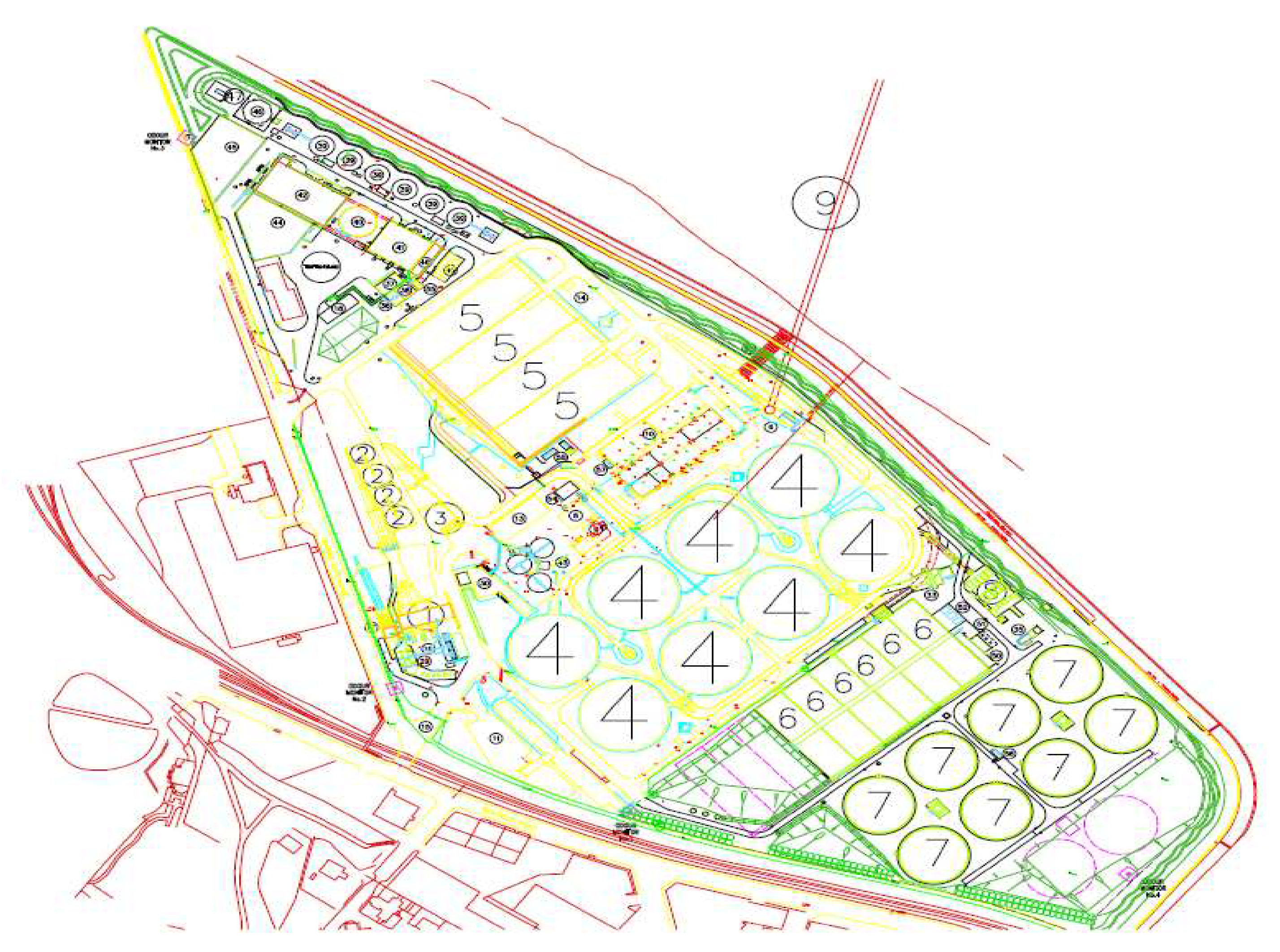
The data to be used is collected from the Seafield Wastewater Treatment Plant (layout shown in Figure 2), located in the eastern part of Edinburgh, United Kingdom, and is Scotland’s largest WWTP, processing 300 million litres of wastewater daily. The plant receives water from the Edinburgh catchment, which contains domestic effluent, industrial discharge, and rainwater. It is a conventional Activated Sludge plant with eight circular sedimentation tanks, four rectangular non-nitrifying aeration lanes, and eight circular final settlement tanks [27]. The data covers an 8-and-a-half-year period from 28 March 2012 to 22 August 2021.
Outliers were identified using the Z-score method (threshold ± 3), a standard statistical technique for detecting anomalous values in environmental datasets [26,27,28]. The Z-scores were calculated based on Equation (1) [29]:
Z x =   x x ¯ σ
where x is the original data value; x ¯ and σ are the average and standard deviation of the variable values. In addition, a modified Z-score approach based on the median and median absolute deviation (MAD) was also applied to ensure robustness for variables with skewed distributions. Observations exceeding a modified Z-score threshold of ±3.5 were also flagged.
Although this is a convenient and simple technique, it is worth noting that it is a univariate analysis that focuses on each variable separately, whereas WWTP data has high correlations between variables, which may be missed by this method [30]. After careful analysis, it was decided that these observations were critical to the data distribution characteristics and removing them entirely would introduce potential bias. In such situations, treating them as missing values and imputing them is a better option [25]. Thus, these observations were treated as missing values and filled in accordance with the following sections. In total, including replaced outliers, there are 25,711 missing values in the dataset, with an average proportion of around 39%, ranging from 0.29% to 92.1%.
Based on the literature review, the following five methods were identified for this study: Amelia II, MICE, MissForest, MissRanger, and KSOM. A summary of the methods is given in Table 1. A short description of each method is also provided in Section 2.2, Section 2.3, Section 2.4 and Section 2.5.

2.2. Amelia II

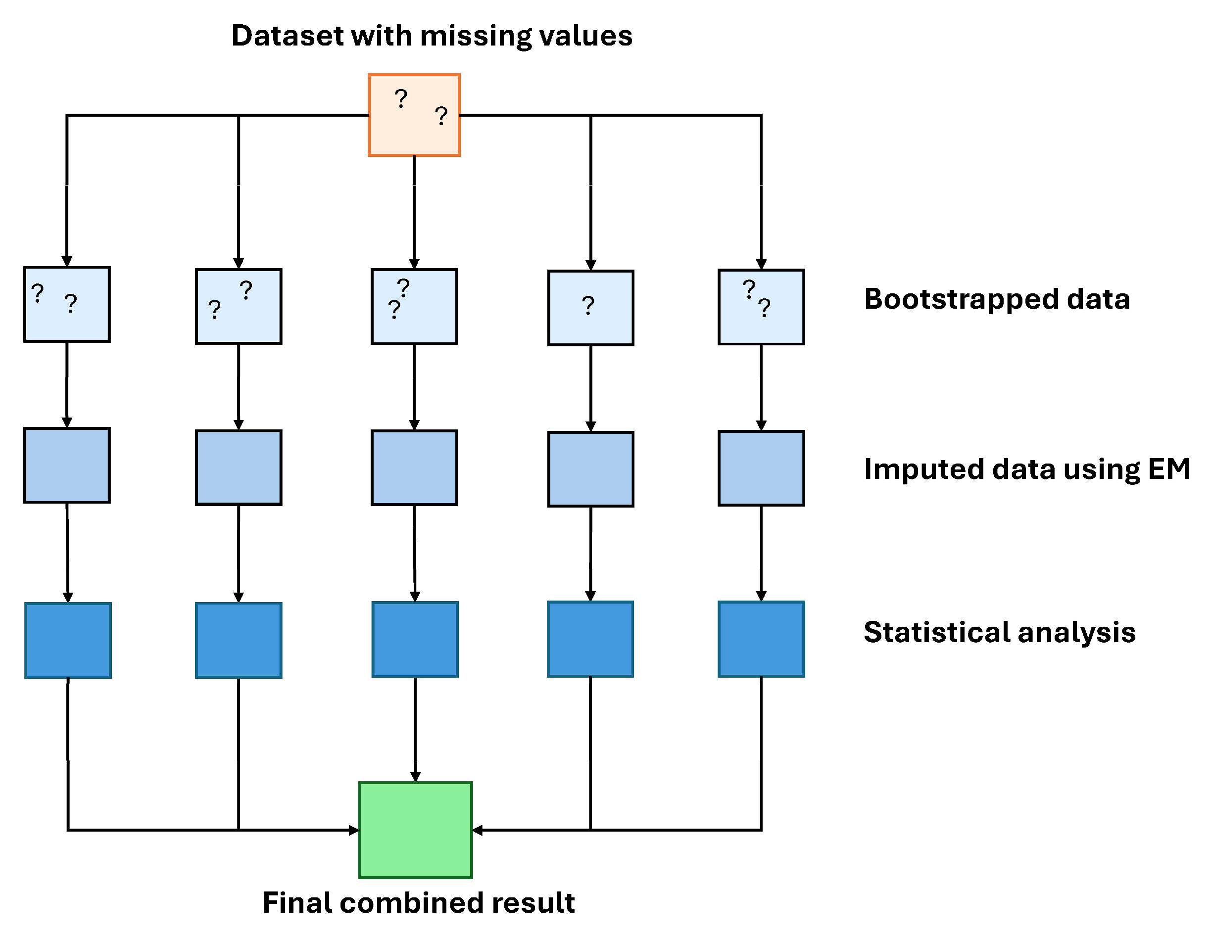
The Amelia II algorithm is an updated version of the Amelia program introduced by Honaker et al. [31]. The program is based on the Expectation-Maximization (EM) algorithm, adapted by King et al. [33] to create a general multiple imputation model. Amelia II extends the original algorithm using a bootstrapping approach and the Expectation-Maximization (EM) algorithm. Compared to the first version, Amelia II can impute more data and variables in less time. It uses the EM on several bootstrapped incomplete-data samples to estimate the to-be-imputed parameter values. Then, values are drawn from each imputed data set to replace missing values, as shown in Figure 3 [31,34]. The method is best used for data missing at random (MAR) and data that, when complete, yield a normal distribution [34]. It differs from other traditional imputation approaches because it assumes that the data will follow a normal distribution and thus uses a joint modelling approach. In contrast, other approaches use a variable-by-variable approach [24]. It can also impute large amounts of data quickly because of the bootstrapping algorithm [35].
The Amelia II algorithm involves the following steps [31]:
Take the input dataset as an n × k matrix denoted by D , with D o b s being the available values and D m i s being the missing values. The assumption that D follows a multivariate normal distribution can be expressed as
D N k ( μ , Σ )
where μ is the mean vector and Σ is the covariance matrix.
Define M as the missing values matrix, where m i j = 1 if d i j ϵ D m i s and m i j = 0 otherwise. Thus, values can be checked as MAR and estimated using Equation (3) [36]:
p D o b s δ = p D δ d | D m i s
where δ = ( μ , Σ ) is the distribution parameter (also called the posterior parameter).
Next, the algorithm generates m samples of size n from matrix D and uses the EM algorithm to produce bootstrapped point estimates of μ and Σ , considering both the conditional distribution of D o b s and the posterior parameter. Then, for each set of estimates, the original sample units are used to impute the missing values in D m i s in their original positions [31,36].

2.3. Multiple Imputation Using Chained Equation (MICE)

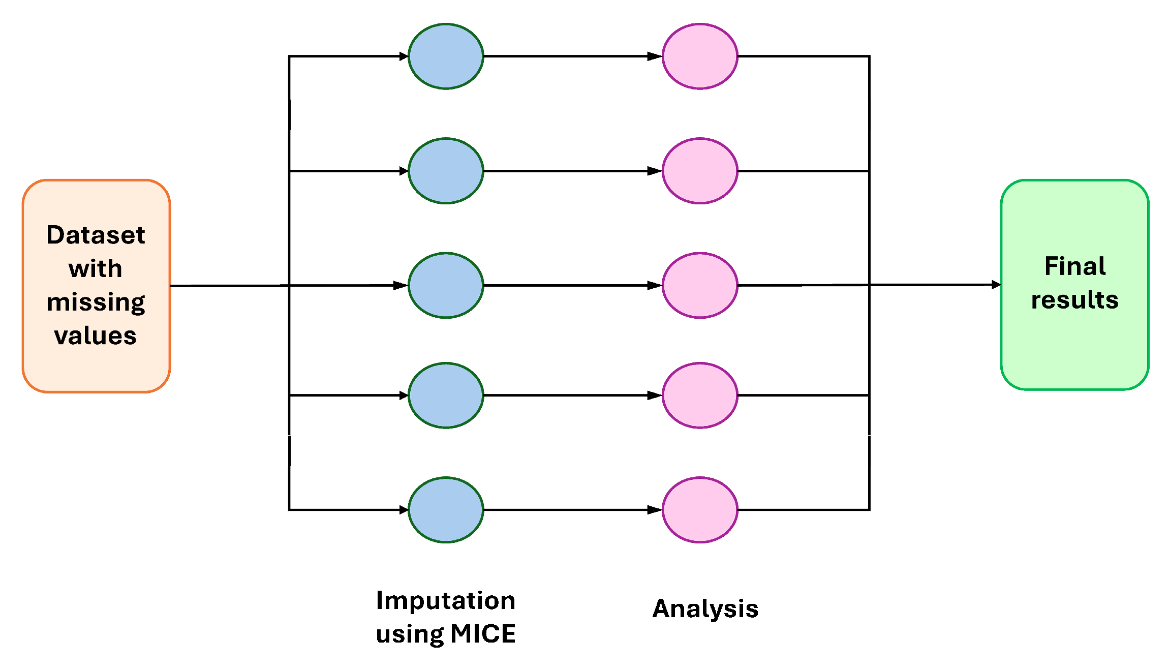
The MICE algorithm, introduced by Stef van Buuren in 2011, is based on Fully Conditional Specification, in which each variable is imputed conditionally on all other variables, and it is primarily used on MAR datasets [37,38,39]. It can be used with continuous, binary, or categorical variables, with each type modelled based on its distribution. It is a Bayesian procedure in which, if there is a known joint distribution (usually a multivariate normal distribution) for the available data and a data model, it is possible to obtain a posterior distribution of the missing values in that data [40]. In this method, each missing variable is treated as a dependent variable, and the other available data are treated as independent variables [39]. An illustration is shown in Figure 4.
The steps involved in the MICE algorithm are given below [41].
Consider two input variables, denoted Y and K , with missing values Y m i s and K m i s , the available values being Y o b s and K o b s . Let Z be a complete matrix, with Z o b s and Z m i s corresponding to available and missing values of Y and K , respectively. Given that Y and K are assumed to be random and that prior distributions are assigned, posterior distributions can be found by performing conditioning on the Z variables.
Initial estimates of missing values of Y and K can then be found with the aid of available values Y o b s and K o b s , using Equations (4) and (5):
Y m i s , i ^ = Y o b s , i n Y o b s
K m i s , i ^ = K o b s , i n K o b s
where n Y o b s and n K o b s are the total number of available values for Y o b s and K o b s , respectively.
Next, the estimate of one of the variables, for example, Y m i s , i ^ , is set back as a missing value.
A linear regression is then fitted between Y o b s and either all or a subset of Z , as in Equation (6):
Y m i s , i ^ = θ T Z
where θ is the row vector of the regression parameters, which can be found by minimizing the Mean Squared Error (MSE), as in Equation (7).
M S E = 1 n Y o b s i = 1 n Y o b s ( Y o b s , i Y o b s , i ^ ) 2
The MSE can be minimized to find θ using either an optimization algorithm or an algebraic approach, with the former preferred for larger datasets to reduce computational time, as in the ASP in this study.
Equation (6) is then used to impute the missing values Y m i s . This process is repeated for every other variable with missing values in the dataset to conclude the first iteration of the algorithm. The algorithm is iterated for a set number of iterations (usually 10) [41].
At the end of imputation, multiple datasets are produced by the iterative nature of the process, which can be analyzed using standard statistical techniques to yield an imputed dataset [39]. For example, if linear regression is used for imputation, the imputed datasets can be evaluated using regression coefficients and standard errors. If θ i is the statistic of interest, e.g., the regression coefficient, from the i t h imputed dataset, then the pooled average estimate of it can be shown as in Equation (8) [38]:
θ = 1 M i = 1 M θ i
where M is the number of imputed datasets.

2.4. MissForest Algorithm

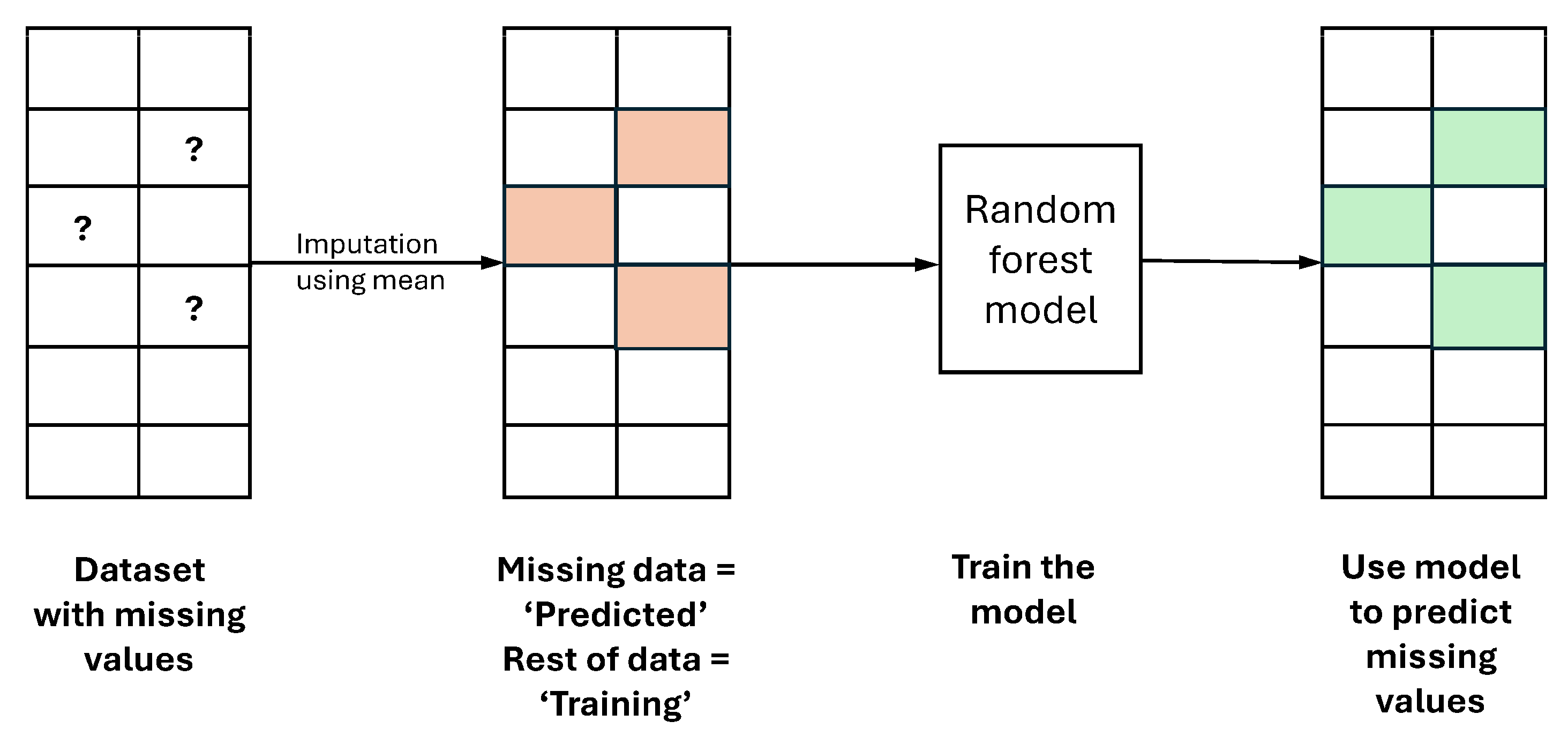
The missForest algorithm is an imputation technique developed by Stekhoven and Bühlmann in 2012 [19], which is based on Random Forests by Breiman [20] and can handle mixed-type data (categorical and numerical) [19,42,43,44]. The only requirement for the algorithm is that the variables applied to it must be pairwise independent [45]. It employs a univariate Fully Conditional Specification (FCS) strategy, using random forests for regression with integer variables or classification with categorical variables [21]. The missForest algorithm is especially good at estimating out-of-bag (OOB) imputation error rates without requiring a test dataset or tuning parameters. It is also possible to reduce imputation error by up to 50% in only a few iterations, making it an attractive option for reducing computational time [19]. ASP data, especially when it contains more missing values, can take a long time to compute imputation algorithms, so missForest is a good option. An illustration is given in Figure 5.
The steps involved in the algorithm are given as follows [19]:
Considering input data X as an n × p matrix, with a stopping criterion γ , an initial guess is made for the missing values using mean imputation or any other method.
For an arbitrary variable X s   ( s = 1 , , p ) with missing values at locations i s m i s { 1 , , n } , available values can be denoted as y s o b s ; missing values can be denoted as y s m i s . Variables other than X s with available values located at i s o b s = { 1 , . , n } \ i s m i s can be denoted as x s o b s , and missing values located at i s m i s can be denoted as x s m i s .
The values of X s can be sorted out starting from the lowest number of missing values. Then, for each variable X s , a random forest with a number of trees n t r e e is fitted with a response y s o b s and predictors x s o b s . This random forest can next be applied to x s m i s to find the missing values y s m i s . This procedure is repeated for all n t r e e until the stopping criterion γ is met to obtain the imputed matrix X i m p . The stopping criterion is met when the difference between X i m p of the current and previous iterations increases for the first time [19,45]. If there are both continuous N and categorical variables F present, the following Equations (9) and (10) can be used to calculate the difference [19]:
N = j N ( X i m p n e w X i m p o l d ) 2 j N ( X i m p n e w ) 2
F = j F ( X i m p n e w X i m p o l d ) 2 # N A
where # N A is the number of missing values in the categorical variables.

2.5. MissRanger Algorithm

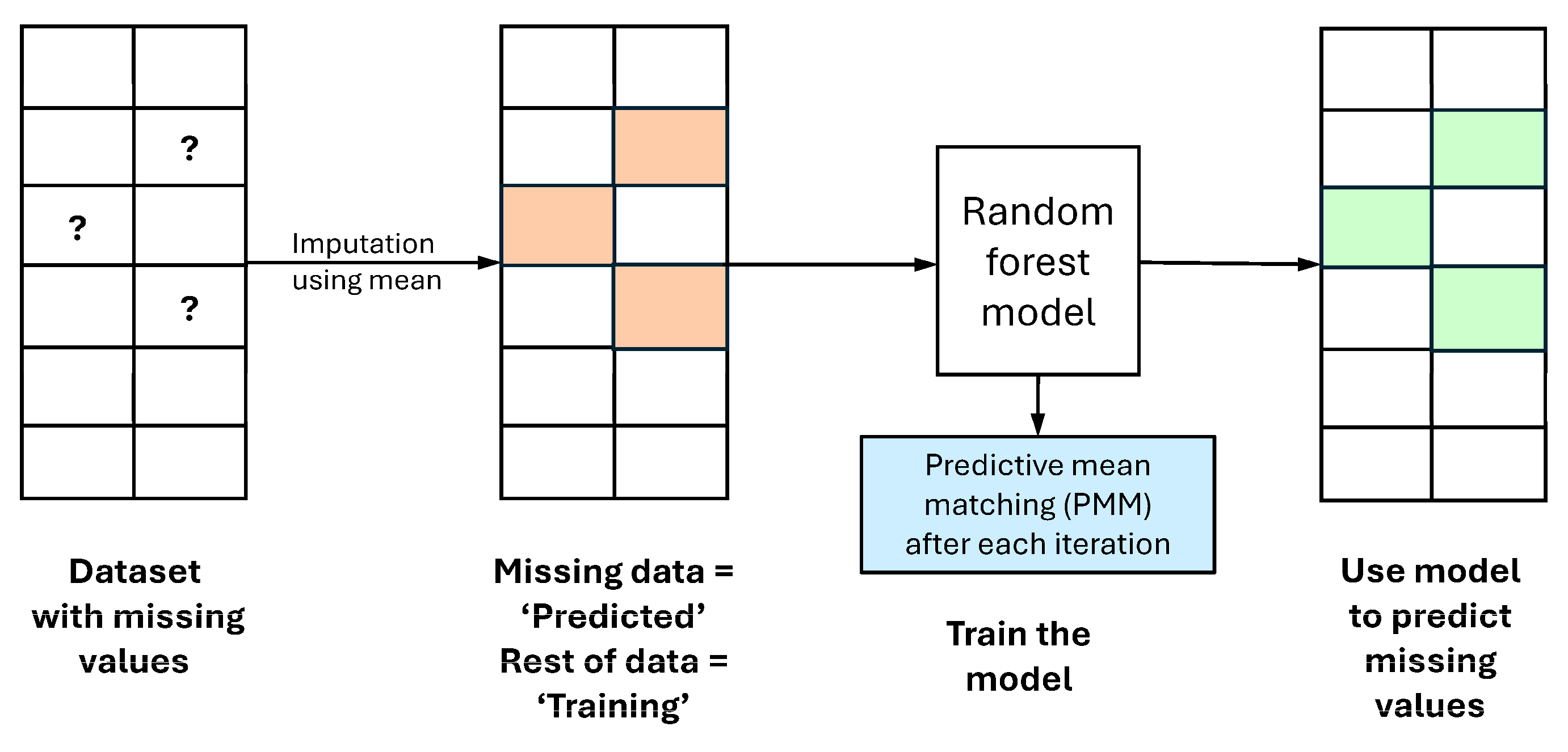
An alternate, faster variation of the MissForest algorithm is the MissRanger algorithm developed by Michael Mayer in 2019. MissRanger performs univariate iterative imputation using chained random forests with an additional option of Predictive mean matching (PMM) added between iterations [21]. PMM is a method by which it is possible to ensure that the imputation algorithm does not introduce imputed values that are not present in the original variable. This can cause distortion in predicted values, e.g., imputed values less than zero in a variable with values greater than zero [21,46]. The PMM process generates predicted mean values for each value in a variable, whether it is missing or not. Then, for each missing value, the available data with the closest predicted mean is replaced by the imputed value, as shown in Figure 6. The PMM technique also helps keep the variance of the imputed values at a realistic level, thereby enabling multiple imputations using the MissRanger algorithm.

2.6. Kohonen Self-Organising Maps (KSOM)

KSOM is an unsupervised artificial neural network algorithm that uses clustering of input data to create a 2-D map or grid, forming a simple relationship between data variables [25,47,48,49]. It was introduced by Teuvo Kohonen in 1981–1982 based on data-driven, unsupervised competitive learning, where within the 2D grid, similar input patterns will be represented by the same output neuron or neighbouring neurons [50,51,52]. Self-organizing maps, compared to traditional neural networks, are useful for pattern recognition, analysis of high-dimensional data, process control, extraction of salient features, and processing semantic information, without the need for data preprocessing [51,53,54].
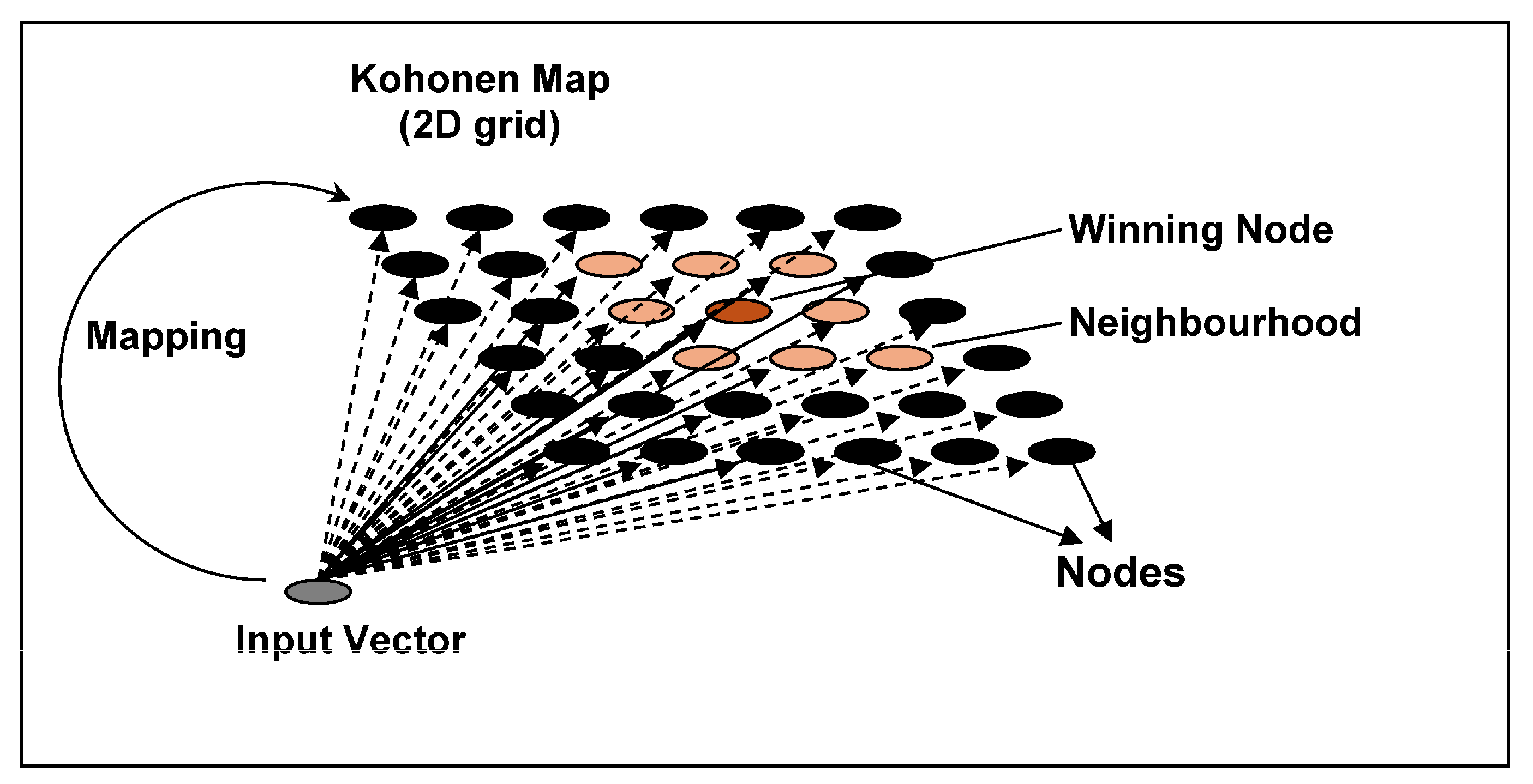
The algorithm consists of two layers: an input layer containing input nodes and a Kohonen output layer containing several connected, weighted computational nodes, referred to as neurons, which form a 2D grid [27,55,56]. Grid size is determined by the number of training data points and can be estimated from the size of the input vector [57,58]. All variables contained in the input vector are also contained in each node of the output layer [59]. The number of neurons affects KSOM’s ability to accurately predict and generalize data [27]. The neurons are activated using a topological function that categorizes each neuron based on its similarity to the input vectors and organizes them into a rectangular or hexagonal grid, as shown in Figure 7 [55,60].
A rectangular grid means that each neuron will be connected to four of its neighbours, whereas a hexagonal grid will have each neuron connected to six of its neighbours [27]. While distances between different neurons might not be equal, the closest neuron is always within its neighbourhood [60]. Input data is applied to the algorithm either sequentially (single input vector at a time) or in a batch (batch-type process), and all models are updated in a single concurrent operation. The input vectors identify similar code vectors using the Euclidean distance, with the minimum distance indicating the Best Matching Unit (BMU). Through this, each node is able to ultimately recognize similar vectors to itself, thereby ‘self-organizing’ [61]. The process is repeated until the model stabilizes [58]. This clustering used in KSOM can then be used to obtain a similar pattern between required outputs and, effectively, reduce the dimensionality and complexity of activated sludge datasets, as needed for this study [60]. Most missing value estimation methods focus on univariate analysis, whereas KSOM can handle correlations among multiple variables, even when there are many missing values, making it a good multivariate approach for imputation [53,62,63,64].
The steps involved in a classic KSOM are given below:
The input data is first normalized by deducting the mean and dividing by the standard deviation. The initial iteration sets the neuron weights to the range {−1, 1}, with a mean of zero and variance of one [64,65]. The number of neurons can be determined using Equation (11) [64,66]:
M = 5 N
where N is the number of data samples.
The number of rows and columns in the KSOM can be determined using Equation (12) [64]:
l 1 l 2 = e 1 e 2
where l 1 and l 2 are the number of rows and columns, e 1 is the biggest eigenvalue of the dataset, and e 2 is the second biggest eigenvalue of the dataset.
A standard input vector is randomly selected and presented to the algorithm, and neurons compete by comparing their weights with the selected vector. The comparison is made by measuring the Euclidean distance, as in Equation (13) [25,27,64]:
D i = j = 1 n ( x j w i j ) 2       i = 1,2 , . , M
where i is the weight vector, x j is the jth element of the input vector, w i j is the jth element of the weight vector, M is the number of neurons, and n is the dimensionality of the input and weight vectors.
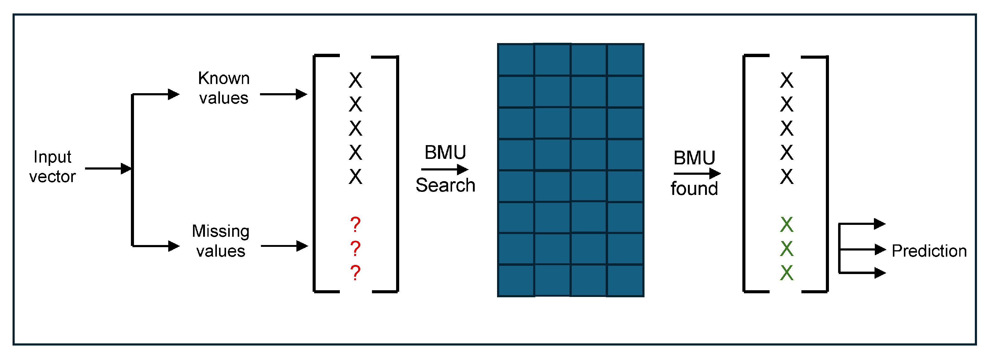
Whichever neuron has the least distance is the most similar to the input neuron and is selected as the Best Matching Unit (BMU), as shown in Figure 8 [25,66]. The neighbourhood radius of the BMU ( σ ( t ) ) is then determined by setting it to the network’s radius. This value decreases with each iteration [67]. Then, the weights of the BMU, as well as neurons within the neighbourhood radius, are modified to bring it closer to the input vector, as in Equation (14):
w i t + 1 = w i t + α ( t ) h c i ( t ) x t w i t
where w i is the weight vector of neuron i at time t; α is the learning rate at time t for training length T , given by Equation (15):
α t = α o 0.005 α o t T
and h c i is the neighbourhood function centred in winning unit c , given by Equation (16):
h c i = exp r c r i 2 2 σ 2 t
where r c and r i are positions of nodes c and i on the KSOM grid.
This process is iterated until the maximum number of iterations specified is reached or the specified error limits are reached [60,67,68]. Once the process is complete, the BMUs can be treated as extracted features of the data, with no outliers or missing values [27,64].
The quality and success of KSOM can be identified using two types of errors [25,27]:
Quantization error is given by Equation (17):
q e = 1 N i = 1 N | X i W c |
where X i is the ith element in the dataset, W c is the prototype vector of BMU for X i and | | . | | stands for the Euclidean distance.
Topographic error is given by Equation (18):
t e = 1 N i = 1 N u ( X i )
where u i is a binary integer that is equal to 1 if the first and second BMUs for X i are not adjacent units and zero if otherwise.

2.7. Algorithm Procedure Details

Each imputation method was applied using default/revised hyperparameters, as shown in Table 2. The default values for some algorithms were modified to meet computational time constraints and obtain results appropriate for the dataset’s size and complexity. The Seafield WWTP dataset contains approximately 3430 rows and 19 variables, with around 25,711 missing values in total (39% average missingness), which places significant demands on iterative algorithms. The modifications made are detailed below.
For MICE, the number of imputed datasets was increased to m = 10 from the default of 5. This was done to improve the stability of the imputed values across all variables, particularly for the variables with a high percentage of missing data, such as RAS volume and RL load. Increasing the m value added approximately 40–50% to the computation time but produced more consistent results. Logged events were also checked using imp$loggedEvents, a diagnostic dataframe within the R package ‘mice’ to identify any warnings during imputation.
For MissForest, both the number of trees and the maximum number of iterations were reduced from their default values. The number of trees was set to ntree = 10, vs. the default of 100, and the maximum iterations to maxiter = 1, vs. the default of 10. The default settings were found to increase computational time by approximately 8 times, which is impractical. While the reduced hyperparameters affect accuracy to some degree, it was necessary to obtain results within a reasonable time period. In comparison, all default values were kept for MissRanger, as the Ranger package used in this method runs faster than the MissForest algorithm. This is discussed further in Section 3.3.
The remaining imputation methods, Amelia II, MICE, MissForest and MissRanger, were implemented in the R statistical computing environment (R version 4.1.0). All analyses were conducted using publicly available R packages, with software versions and key hyperparameters summarized in Table 2. Detailed package references and version information are provided in the Supplementary Materials.

2.8. Algorithm Evaluation Criteria

The performance of each algorithm was evaluated based on the following metrics, where x i refers to observed values, x i refers to predicted values, and N refers to the number of data points [27].
The coefficient of determination is given by Equation (19).
R 2 = 1 i = 1 N ( x i x i ) 2 i = 1 N ( x i x ¯ ) 2
Average Absolute Error computes the mean error of the predicted values rather than the observed values, as given by Equation (20).
A A E = 1 N i = 1 N ( x i x i )
Relative Average Absolute Error (RAAE) computes the AAE and scales it by the data range, as given by Equation (21). To check the accuracy of any imputation model, this value should be as close to zero as possible [27].
R A A E = A A E M a x x M i n ( x )
Mean Squared Error (MSE) provides the average of the squared difference between the predicted and observed values, given by Equation (22).
M S E = 1 N i = 1 N ( x i x i ) 2
Root Mean Squared Error (RMSE) provides the sample standard deviation of the difference between the predicted and observed values, given by Equation (23).
R M S E = M S E = 1 N i = 1 N ( x i x i ) 2

2.9. Validation and Testing

It is necessary to validate the imputed values generated by the algorithms, since their original values are unavailable for cross-checking. This is a common challenge in methods for imputing missing data. The following validation procedure based on held-out observed values is followed in this study:
Masking of observed data
For each variable, a subset of the originally observed non-missing data was randomly selected and temporarily treated as missing to form a test dataset. Masking was performed independently for each variable, preserving the original dataset’s temporal order.
Imputation
Each imputation method was applied to the dataset containing both the original missing values and the additional masked values. For multiple IMs such as MICE, the mean of the imputed values across all imputations was used as the final predicted value. For single IMs like KSOM, the directly imputed value was used as the predicted value.
Repetition
To reduce the effect of randomness in the masking process, the procedure was repeated 3 times using different random seeds. The final performance metrics given are the average values obtained across all repetitions.
Performance evaluation
All evaluation metrics were calculated for the held-out observed values by comparing the imputed values with the original masked observed values. This held-out observed approach is the standard way to ensure that the values obtained are unbiased when the true values for originally missing entries are unavailable. It measures how well each method can impute known values under realistic masking and therefore provides a fair basis for comparison of different algorithms.

3. Results

The methods used—KSOM, Amelia II, MICE, MissForest, and MissRanger—were compared primarily based on the coefficient of determination (R2). Other metrics are shown in the Supplementary Materials, including average absolute error (AAE), relative average absolute error (RAAE), mean squared error (MSE), and root mean squared error (RMSE).

3.1. Outlier Detection and Treatment

Before data imputation, outliers in the dataset were identified and treated as missing values to prevent extreme values in the data from biasing the imputation results. Given the variability and potential skewness in WWTP data, two complementary methods were used for outlier detection: the standard Z-score method and the modified Z-score method.
The Z-score method identifies outliers based on the mean and standard deviation of each variable, with a threshold of ±3 used in this study. The modified Z-score method, which is based on the median and median absolute deviation (MAD), was also applied to improve robustness for variables with non-normal distributions. A threshold of ±3.5 was used for the modified Z-score.
Table 3 presents the number of outliers detected for each variable using the two methods. It can be observed that the number of detected outliers varies significantly across methods. In general, the modified Z-score identifies more outliers than the standard Z-score method, particularly for variables with high variability or skewed distributions. For example, variables such as ML SSVI, Food, and F/M exhibit significantly more outliers when using the modified Z-score, indicating strong deviations from normality. In contrast, variables such as SAS volume and RAS volume show no detected outliers across the methods, suggesting either stable measurements or a high proportion of constant or zero values.
The standard Z-score method was selected as the primary criterion for outlier removal in this study. This choice was made to maintain consistency across variables and avoid excessive removal of data points, which could further increase the already high level of missingness in the dataset. While the modified Z-score is more sensitive to distributional irregularities, it was used here primarily for comparative analysis and to confirm the presence of extreme values. All data points identified as outliers using the Z-score method were removed and treated as missing values prior to imputation. This preprocessing step resulted in a dataset that preserves the overall structure and variability of the process while minimizing the influence of extreme or potentially erroneous observations.
The combined effect of original missing values and outlier removal accounts for approximately 39% of the overall missingness in the dataset. This highlights the practical challenges of real-world WWTP data and reinforces the need for robust imputation techniques that can handle high and uneven rates of missingness.

3.2. Linear Regression

To provide a simple benchmark against which the performance of other imputation methods can be assessed, a linear regression (LR)-based imputation approach was implemented as a baseline model. In this method, the variable Final effluent COD was treated as the response variable, and all available process variables were used as predictors. The model was trained using only the observed non-missing data. Missing values in the response variable were then estimated using the fitted regression model. The LR model was generated using Excel’s Data Analysis function.
To ensure consistency with the evaluation framework used for all imputation methods, the same held-out validation strategy described in Section 2.9 was applied. A subset of observed values was randomly masked. The regression model was trained on the remaining data. Predictions were compared against the held-out true values. Metrics were computed over multiple repetitions.
The performance of the LR model is summarised in Table 4.
The linear regression model achieved a moderate coefficient of determination (R2 = 0.49), indicating that approximately half of the variance in Final Effluent COD can be explained by linear relationships with the available predictors.
However, compared to the other imputation methods evaluated in this study, the baseline approach exhibits several limitations, such as limited ability to capture nonlinear behaviour in the ASP, reduced performance under high and uneven missingness, and higher prediction errors, as reflected in RMSE and MSE values.
These results confirm that while linear regression provides a useful reference point, it is insufficient for accurately imputing complex, multivariate WWTP data. This highlights the added value of methods such as KSOM, MICE, and tree-based approaches.

3.3. Sensitivity Analysis

A sensitivity analysis was conducted to assess the effects of key hyperparameters on each algorithm’s performance. Since re-running all algorithms across the full range of hyperparameter combinations is impractical, the existing literature is used to determine the sensitivity analysis based on the dataset characteristics.
For Amelia II, the number of imputations (m) was set to 1 in this study. In general, increasing m from 1 to 5 is expected to reduce variability in the imputed values and produce more stable R2 values, particularly for the variables with high missingness. Honaker et al. [35] recommend m ≥ 5 for datasets with more than 30% missing data. For this dataset, it is found that increasing m to 5 would improve R2 values by approximately 0.03–0.08 for variables such as RAS volume and RL SS, which have the highest percentage of missing values. However, as the primary objective here was comparison of methods rather than optimization of a single method; m = 1 was considered adequate for this purpose.
For MICE, m was set to 10 in this study. Based on findings in the literature [38], increasing m beyond 10 yields diminishing returns in imputation accuracy for datasets of this size. White et al. [69] suggest that m should be at least equal to the percentage of missing data. For this dataset with 39% missingness, this suggests m = 10 is on the lower end. However, m = 20 reduces variability in R2 values by around 0.01–0.03, at the cost of doubling the computational time. The current setting of m = 10 is thus considered reasonable.
The most significant modification to the study hyperparameters was for MissForest, where ntree was reduced from the default 100 to 10 and maxiter from 10 to 1. Based on Stekhoven and Buhlmann [19], reducing the ntree value is expected to decrease imputation accuracy by about 15–25% for continuous variables, as fewer trees reduce the stability of the random forest predictions. This is consistent with the results in Table 5, where MissRanger outperforms MissForest despite the two being similar tree-based algorithms. Running MissForest with default parameters might improve its performance closer to that of MissRanger, but at the cost of computational time, as mentioned earlier in Section 2.7.
For MissRanger, the default hyperparameter values were used with no changes. The ntree value used was 500, which could be reduced further; however, according to Hasyyati and Lumley [70], a decrease from 500 to 100 would not significantly affect imputation accuracy but would reduce computational time. In this study, it was still faster than MissForest, so the ntree value was kept at 500.
For KSOM, the map size (22 × 13) was determined from the data using Equations (11) and (12). Rustum and Adeloye [25] found that increasing the map size beyond the values obtained from the equations yields only a small improvement in quantization error while significantly increasing computational time. Therefore, the map size used is considered reasonable for this dataset.

3.4. Comparative Performance of Algorithms

All methods except KSOM perform poorly in imputation, with low R2 values—Amelia II has the lowest performance and MissRanger performs well on a few variables. This could be due to the relatively large number of missing values within each variable. For example, Return Liquor Suspended Solids and Return Liquor Load have around 70% missing values, for which Amelia II, MICE, MissForest and MissRanger have very low R2 coefficients, whereas KSOM has R2 coefficients closer to 1. In a study by Nijim and Rustum [26], it was concluded that when missing values are less than 20%, KSOM is an accurate method, but for more than 40% of missing data, KSOM performs poorly. In Table 5, the Return Activated Sludge volume has the highest percentage of missing values and shows the worst performance among the other imputation methods, except KSOM. Garciarena and Santana [17] stated that when choosing an imputation method, looking at data characteristics is unnecessary. KSOM is clearly a better approach in this dataset. Both Garciarena and Santana [17] and Nijim and Rustum [26] also found that as the percentage of missing data increased, performance weakened across all methods. In this study, it is noted that the Mixed Liquor Sludge Volume Index has a lower percentage of missing values (around 25%) and yields relatively high R2 coefficients across all methods. As per Casiraghi et al. [21], across all methods, the higher the number of imputations, the more stable the algorithm became, especially for the MissRanger algorithm. Increasing the number of imputations might provide better results in this study. Detailed performance metrics and dataset statistics are provided in the Supplementary Materials.
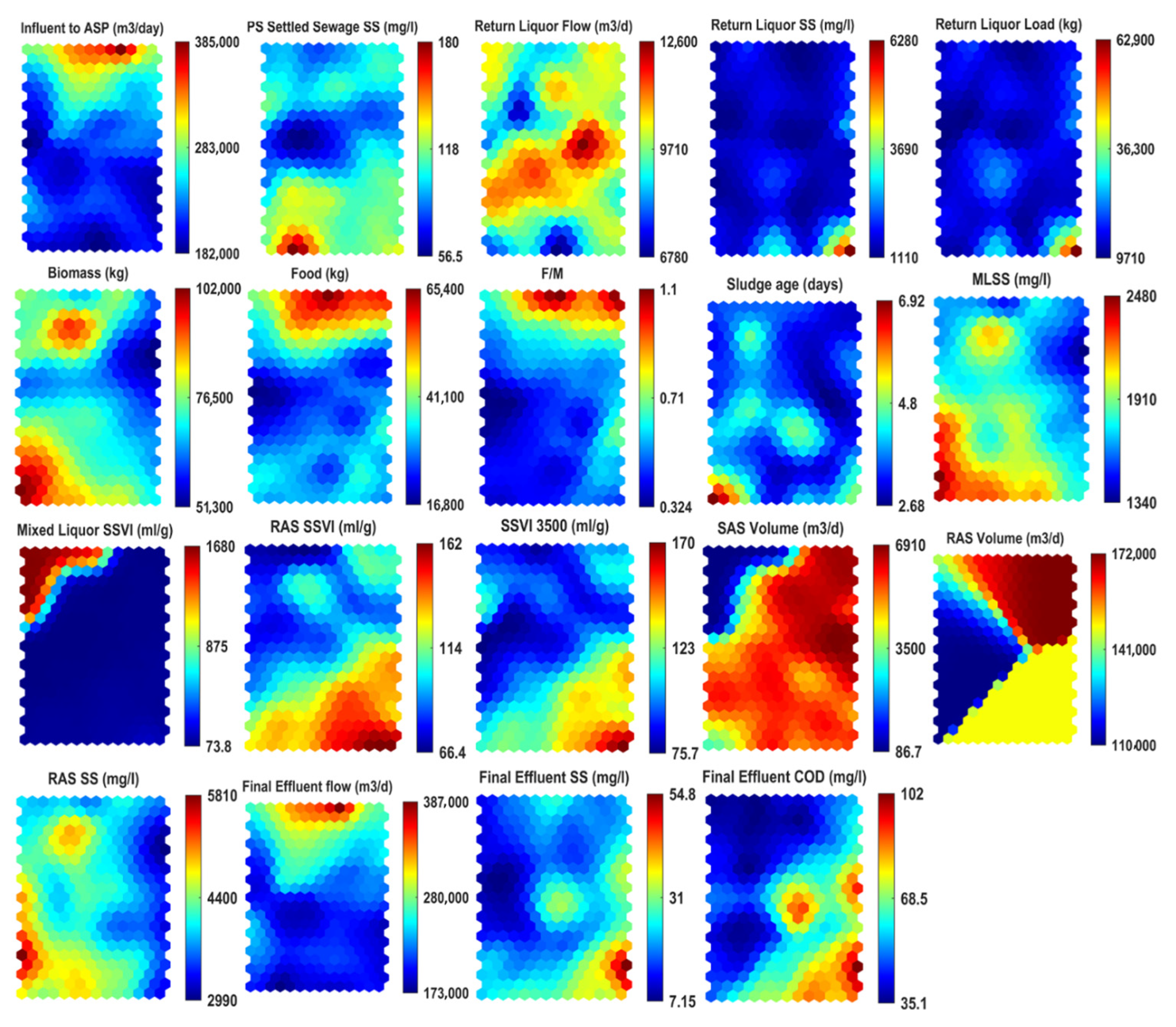
One advantage of the KSOM method is the ability to visualize correlations among variables using component planes [25,47]. The component planes of each variable for KSOM are given in Figure 9. The component plane for each variable consists of hexagonal units, and their values are shown according to the colour codes (low = blue, high = red), shown adjacent to them. The KSOM component planes reveal several relationships consistent with conventional activated sludge behaviour. Higher influent regions coincide with increased food loading and higher F/M ratios, while MLSS and sludge age are comparatively lower, indicating that the treatment process occurs at a higher rate. Biomass, MLSS and sludge age are positively correlated to each other, which indicates stable operating conditions. Effluent quality shows expected trends, where final effluent COD and suspended solids increase in regions associated with higher F/M and reduced solids retention. Also, return sludge (RAS) flow shows a negative correlation with RAS suspended solids, which is as expected due to dilution effects at higher flow rates. Similarly, other relationships can be highlighted from the component planes.
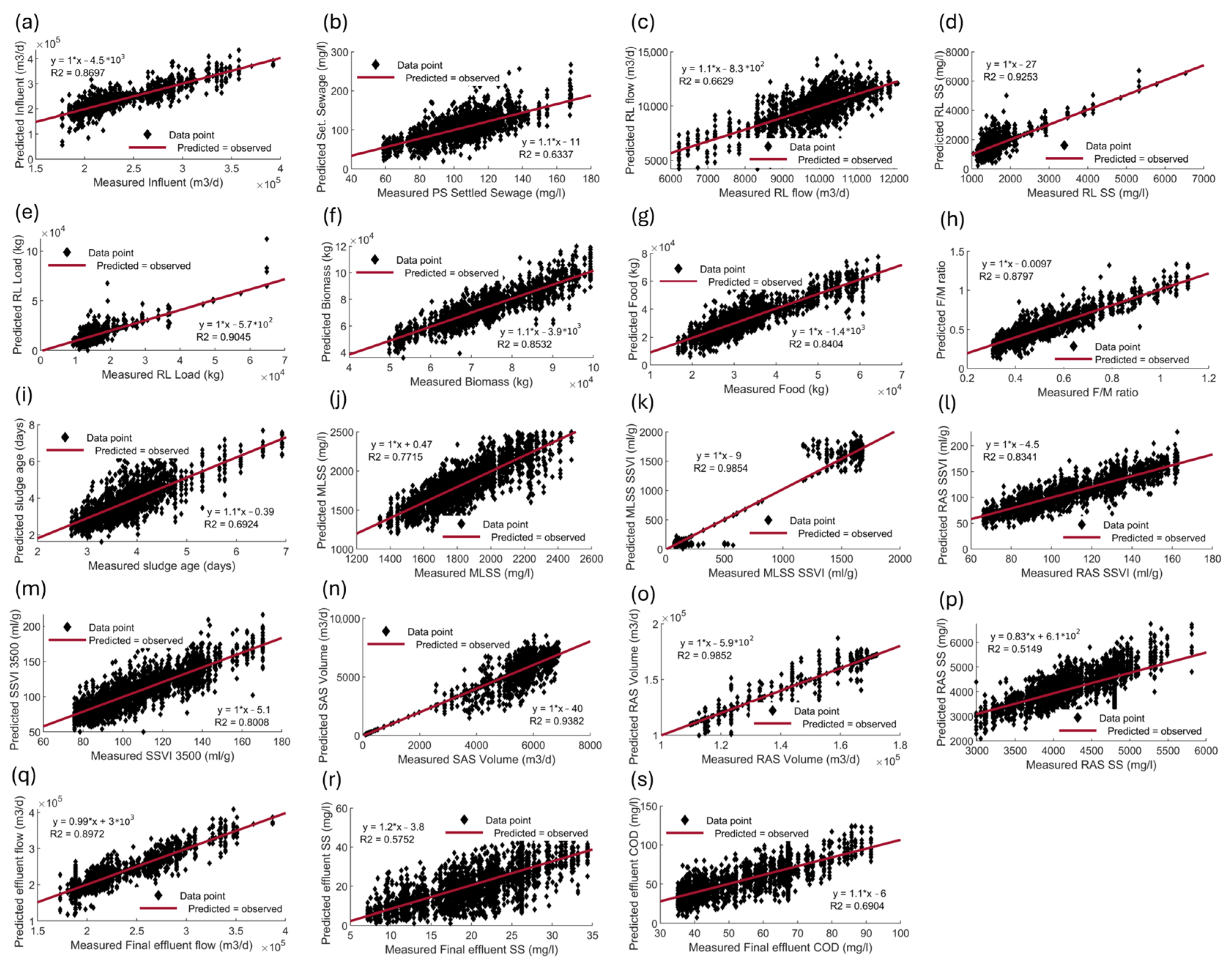
Figure 10 shows the scatter plots for individual variables for the KSOM method. It is clear from the figures that KSOM has a good linear correlation of measured and predicted data points, even for the variables that have a high percentage of missing values.
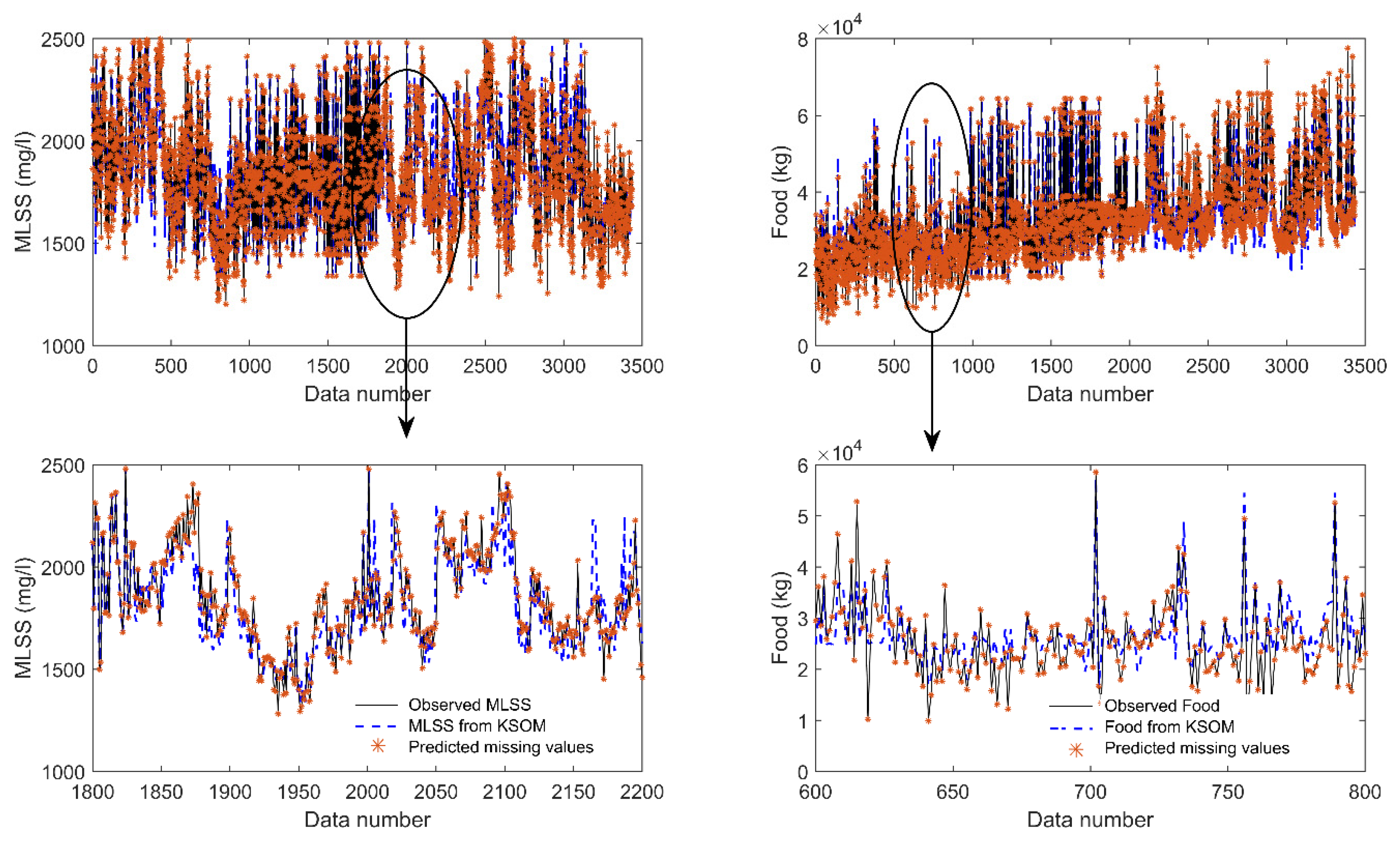
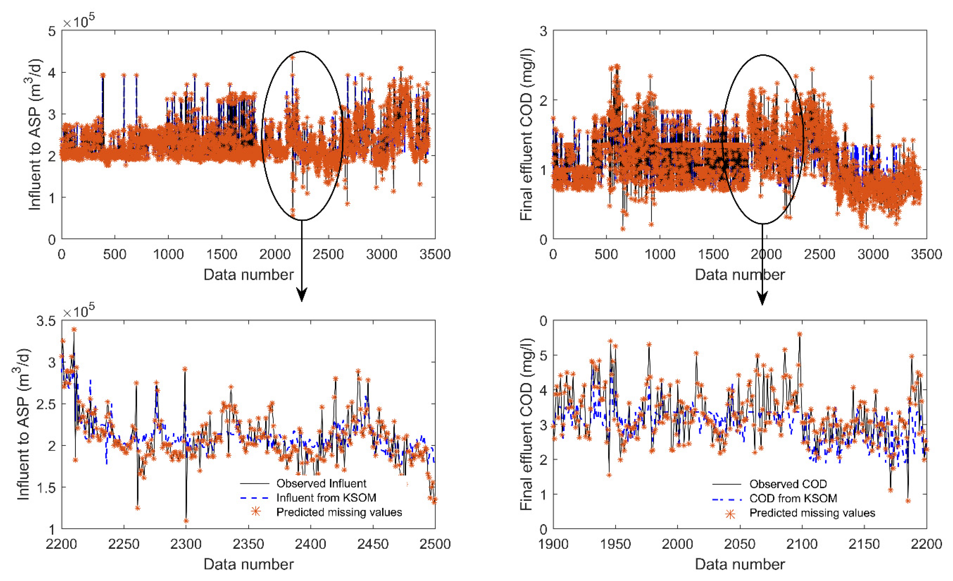
For KSOM, time series plots are given in Figure 11 and Figure 12 for four process variables, namely, Influent to ASP, Final effluent COD, MLSS, and Food, with an additional zoomed-in look at select sections of the graphs to show the efficiency of predicting the missing variables. For example, for RL flow the KSOM values, including predicted missing values, follow the general trend of the observed values’ highs and lows. This indicates KSOM’s good performance.
Also, according to the literature, when the missing data rate is below 40%, KSOM is a suitable method. This dataset has 39% missing data, which is borderline; however, it is also identified through a review that no matter the method used, the results will show if the method is appropriate. The results are checked once imputed to ensure that KSOM is indeed appropriate and that the imputation error is negligible.

3.5. Input Importance Analysis

To assess the influence of input variables on imputation performance, a permutation-based input importance analysis was conducted for the best-performing method, KSOM. As KSOM is an unsupervised, clustering-based algorithm, model-specific tools like SHapley Additive exPlanations (SHAP) are not directly applicable. Each input variable was permuted independently, and the resulting increase in imputation error (RMSE) was quantified for selected target variables. Variables whose permutation caused the largest deterioration in performance were interpreted as having greater importance.
Results indicate that flow-related variables (Influent flow), biomass-related variables (MLSS and Biomass), and load-related variables (Food and COD) exert the strongest influence on imputation accuracy. This aligns with established relationships in the ASP, where hydraulic loading and biomass concentration strongly govern process dynamics.

4. Conclusions

This study evaluated five imputation methods—Kohonen Self-Organising Maps (KSOM), Amelia II, MICE, MissForest, and MissRanger—using a real-world activated sludge plant dataset with 19 process variables and a high level of missing data (approximately 39%). The aim was to assess the suitability of different imputation techniques for handling large and uneven missingness in operational wastewater treatment plant data. Out of the five methods, KSOM achieved the best performance in predicting missing values, with higher R2 values and lower error metrics across most variables. These results support and extend findings from previous studies, confirming that KSOM is well suited for use in complex, multivariate activated sludge plant datasets. Nevertheless, it was observed that for a limited number of variables (6 out of 19), KSOM achieved moderate R2 values (0.5–0.6), indicating that further refinement may be needed before these variables can be reliably used in real-time operational control applications. Future research should therefore focus on enhancing KSOM performance through hybrid approaches, such as combining KSOM with ensemble tree-based algorithms. The fully imputed dataset can now serve as a reliable foundation for developing data-driven ASP models. These models can then be optimized using various techniques, including neural computing and nature-inspired optimization algorithms.

Supplementary Materials

The following supporting information can be downloaded at https://www.mdpi.com/article/10.3390/waste4020017/s1: Table S1: Summary statistics of Seafield WWTP data; Table S2: Proportion of missing data in the dataset; Table S3. Average Absolute Error (AAE) for methods used; Table S4. Relative Average Absolute Error (RAAE) for methods used; Table S5. Mean Squared Error (MSE) for methods used; Table S6. Root Mean Squared Error (RMSE) for methods used; Table S7. Correlation matrix for KSOM.

Author Contributions

Conceptualization, M.D. and R.R.; methodology, M.D. and R.R.; writing—original draft preparation, M.D.; writing—review and editing, R.R.; supervision, R.R. All authors have read and agreed to the published version of the manuscript.

Funding

This research received no external funding.

Institutional Review Board Statement

Not applicable.

Data Availability Statement

The original contributions presented in this study are included in the article. Further inquiries can be directed to the corresponding author.

Acknowledgments

The authors would like to thank their institutions for giving them the time to work on this paper.

Conflicts of Interest

The authors declare no conflicts of interest.

References

  1. Delanka-Pedige, H.M.K.; Munasinghe-Arachchige, S.P.; Abeysiriwardana-Arachchige, I.S.A.; Nirmalakhandan, N. Wastewater infrastructure for sustainable cities: Assessment based on UN sustainable development goals (SDGs). Int. J. Sustain. Dev. World Ecol. 2021, 28, 203–209. [Google Scholar] [CrossRef]
  2. Obaideen, K.; Shehata, N.; Sayed, E.T.; Abdelkareem, M.A.; Mahmoud, M.S.; Olabi, A.G. The role of wastewater treatment in achieving sustainable development goals (SDGs) and sustainability guideline. Energy Nexus 2022, 7, 100112. [Google Scholar] [CrossRef]
  3. Qadir, M.; Drechsel, P.; Jiménez Cisneros, B.; Kim, Y.; Pramanik, A.; Mehta, P.; Olaniyan, O. Global and regional potential of wastewater as a water, nutrient and energy source. Nat. Resour. Forum 2020, 44, 40–51. [Google Scholar] [CrossRef]
  4. Tortajada, C. Contributions of recycled wastewater to clean water and sanitation Sustainable Development Goals. NPJ Clean Water 2020, 3, 22. [Google Scholar] [CrossRef]
  5. Lofrano, G.; Brown, J. Wastewater management through the ages: A history of mankind. Sci. Total Environ. 2010, 408, 5254–5264. [Google Scholar] [CrossRef]
  6. Newhart, K.B.; Holloway, R.W.; Hering, A.S.; Cath, T.Y. Data-driven performance analyses of wastewater treatment plants: A review. Water Res. 2019, 157, 498–513. [Google Scholar] [CrossRef]
  7. Ballhysa, N.; Kim, S.; Byeon, S. Wastewater Treatment Plant Control Strategies. Int. J. Adv. Smart Converg. 2020, 9, 16–25. Available online: https://www.kci.go.kr/kciportal/ci/sereArticleSearch/ciSereArtiView.kci?sereArticleSearchBean.artiId=ART002667271 (accessed on 19 May 2026).
  8. Dürrenmatt, D.J.Ô.; Gujer, W. Data-driven modeling approaches to support wastewater treatment plant operation. Environ. Model. Softw. 2012, 30, 47–56. [Google Scholar] [CrossRef]
  9. Han, H.; Zhu, S.; Qiao, J.; Guo, M. Data-driven intelligent monitoring system for key variables in wastewater treatment process. Chin. J. Chem. Eng. 2018, 26, 2093–2101. [Google Scholar] [CrossRef]
  10. Wang, G.; Zhao, Y.; Liu, C.; Qiao, J. Data-Driven Robust Adaptive Control with Deep Learning for Wastewater Treatment Process. IEEE Trans. Ind. Inform. 2023, 20, 149–157. [Google Scholar] [CrossRef]
  11. Deepak, M.; Rustum, R. Review of Latest Advances in Nature-Inspired Algorithms for Optimization of Activated Sludge Processes. Processes 2022, 11, 77. [Google Scholar] [CrossRef]
  12. Zhang, S.; Jin, Y.; Chen, W.; Wang, J.; Wang, Y.; Ren, H. Artificial intelligence in wastewater treatment: A data-driven analysis of status and trends. Chemosphere 2023, 336, 139163. [Google Scholar] [CrossRef]
  13. Bahramian, M.; Dereli, R.K.; Zhao, W.; Giberti, M.; Casey, E. Data to intelligence: The role of data-driven models in wastewater treatment. Expert Syst. Appl. 2023, 217, 119453. [Google Scholar] [CrossRef]
  14. Khurshid, A.; Pani, A.K. Machine learning approaches for data-driven process monitoring of biological wastewater treatment plant: A review of research works on benchmark simulation model No. 1(BSM1). Environ. Monit. Assess. 2023, 195, 916. [Google Scholar] [CrossRef]
  15. Ly, Q.V.; Truong, V.H.; Ji, B.; Nguyen, X.C.; Cho, K.H.; Ngo, H.H.; Zhang, Z. Exploring potential machine learning application based on big data for prediction of wastewater quality from different full-scale wastewater treatment plants. Sci. Total Environ. 2022, 832, 154930. [Google Scholar] [CrossRef]
  16. Alvi, M.; Batstone, D.; Mbamba, C.K.; Keymer, P.; French, T.; Ward, A.; Dwyer, J.; Cardell-Oliver, R. Deep learning in wastewater treatment: A critical review. Water Res. 2023, 245, 120518. [Google Scholar] [CrossRef]
  17. Garciarena, U.; Santana, R. An extensive analysis of the interaction between missing data types, imputation methods, and supervised classifiers. Expert Syst. Appl. 2017, 89, 52–65. [Google Scholar] [CrossRef]
  18. van Buuren, S.; Groothuis-Oudshoorn, K. Mice: Multivariate imputation by chained equations in R. J. Stat. Softw. 2011, 45, 1–67. [Google Scholar] [CrossRef]
  19. Stekhoven, D.J.; Bühlmann, P. MissForest—Non-parametric missing value imputation for mixed-type data. Bioinformatics 2012, 28, 112–118. [Google Scholar] [CrossRef] [PubMed]
  20. Breiman, L. Random Forests. Mach. Learn. 2001, 45, 5–32. [Google Scholar] [CrossRef]
  21. Casiraghi, E.; Wong, R.; Hall, M.; Coleman, B.; Notaro, M.; Evans, M.D.; Tronieri, J.S.; Blau, H.; Laraway, B.; Callahan, T.J.; et al. A method for comparing multiple imputation techniques: A case study on the U.S. National COVID Cohort Collaborative. J. Biomed. Inform. 2023, 139, 104295. [Google Scholar] [CrossRef]
  22. Suh, H.; Song, J. A comparison of imputation methods using machine learning models. Commun. Stat. Appl. Methods 2023, 30, 331–341. [Google Scholar] [CrossRef]
  23. Chmielowski, K.; Bedla, D.; Dacewicz, E.; Jurik, L. Effect of parametric uncertainty of selected classification models and simulations of wastewater quality indicators on predicting the sludge volume index. Pol. J. Environ. Stud. 2020, 29, 1101–1110. [Google Scholar] [CrossRef]
  24. Kim, W.; Cho, W.; Choi, J.; Kim, J.; Park, C.; Choo, J. A Comparison of the Effects of Data Imputation Methods on Model Performance. In 2019 21st International Conference on Advanced Communication Technology (ICACT); IEEE: Piscataway, NJ, USA, 2019; pp. 592–599. [Google Scholar] [CrossRef]
  25. Rustum, R.; Adeloye, A.J. Replacing Outliers and Missing Values from Activated Sludge Data Using Kohonen Self-Organizing Map. J. Environ. Eng. 2007, 133, 909–916. [Google Scholar] [CrossRef]
  26. Nijim, H.; Rustum, R. Imputation of outliers and missing values for activated sludge dissolved oxygen database using multivariate imputation by chained equations (mice). In Proceedings of the 8th International Conference on Structure, Engineering and Environment, Yokkaichi, Japan, 10–12 November 2022. [Google Scholar]
  27. Rustum, R. Modelling Activated Sludge Wastewater Treatment Plants Using Artificial Intelligence Techniques (Fuzzy Logic and Neural Networks). Doctoral Dissertation, Heriot-Watt University, Edinburgh, UK, 2009. [Google Scholar]
  28. Kowarik, A.; Templ, M. Imputation with the R package VIM. J. Stat. Softw. 2016, 74, 1–16. [Google Scholar] [CrossRef]
  29. Borzooei, S.; Miranda, G.H.B.; Teegavarapu, R.; Scibilia, G.; Meucci, L.; Zanetti, M.C. Assessment of weather-based influent scenarios for a WWTP: Application of a pattern recognition technique. J. Environ. Manag. 2019, 242, 450–456. [Google Scholar] [CrossRef]
  30. Robinson, R.B.; Cox, C.D.; Odom, K. Identifying Outliers in Correlated Water Quality Data. J. Environ. Eng. 2005, 131, 651–657. [Google Scholar] [CrossRef]
  31. Honaker, J.; King, G.; Blackwell, M. Amelia II: A program for missing data, R package version 1.5., 2012. J. Stat. Softw. 2011, 45, 1–47. [Google Scholar] [CrossRef]
  32. Kohonen, T. The self-organizing map. Proc. IEEE 1990, 78, 1464–1480. [Google Scholar] [CrossRef] [PubMed][Green Version]
  33. King, G.; Honaker, J.; Joseph, A.; Scheve, K. Analyzing incomplete political science data: An alternative algorithm for multiple imputation. Am. Political Sci. Rev. 2001, 95, 49–69. [Google Scholar] [CrossRef]
  34. Woldesellasse, H.; Tesfamariam, S. Handling Incomplete and Missing Data in Corrosion Pit Measurement Database Using Imputation Methods: Model Development Using Artificial Neural Network. J. Pipeline Syst. Eng. Pract. 2021, 12, 04021033. [Google Scholar] [CrossRef]
  35. Mabungane, S.; Ramroop, S.; Mwambi, H. Analysis of Missing Data in Progressed Learners: The Use of Multiple Imputation Methods. Afr. J. Res. Math. Sci. Technol. Educ. 2023, 27, 112–122. [Google Scholar] [CrossRef]
  36. Kabir, G.; Tesfamariam, S.; Hemsing, J.; Sadiq, R. Handling incomplete and missing data in water network database using imputation methods. Sustain. Resilient Infrastruct. 2020, 5, 365–377. [Google Scholar] [CrossRef]
  37. Alruhaymi, A.Z.; Kim, C.J. Why Can Multiple Imputations and How (MICE) Algorithm Work? Open J. Stat. 2021, 11, 759–777. [Google Scholar] [CrossRef]
  38. Austin, P.C.; White, I.R.; Lee, D.S.; van Buuren, S. Missing Data in Clinical Research: A Tutorial on Multiple Imputation. Can. J. Cardiol. 2021, 37, 1322–1331. [Google Scholar] [CrossRef]
  39. Khan, S.I.; Hoque, A.S.M.L. SICE: An improved missing data imputation technique. J. Big Data 2020, 7, 37. [Google Scholar] [CrossRef] [PubMed]
  40. Resche-Rigon, M.; White, I.R. Multiple imputation by chained equations for systematically and sporadically missing multilevel data. Stat. Methods Med. Res. 2018, 27, 1634–1649. [Google Scholar] [CrossRef]
  41. Cheliotis, M.; Gkerekos, C.; Lazakis, I.; Theotokatos, G. A novel data condition and performance hybrid imputation method for energy efficient operations of marine systems. Ocean Eng. 2019, 188, 106220. [Google Scholar] [CrossRef]
  42. Jin, H.; Jung, S.; Won, S. missForest with feature selection using binary particle swarm optimization improves the imputation accuracy of continuous data. Genes Genom. 2022, 44, 651–658. [Google Scholar] [CrossRef] [PubMed]
  43. Waljee, A.K.; Mukherjee, A.; Singal, A.G.; Zhang, Y.; Warren, J.; Balis, U.; Marrero, J.; Zhu, J.; Higgins, P.D.R. Comparison of imputation methods for missing laboratory data in medicine. BMJ Open 2013, 3, e002847. [Google Scholar] [CrossRef]
  44. Zhang, S.; Gong, L.; Zeng, Q.; Li, W.; Xiao, F.; Lei, J. Imputation of GPS coordinate time series using MissForest. Remote Sens. 2021, 13, 2312. [Google Scholar] [CrossRef]
  45. Ballesteros, X.M. Comparative Study of Missing Data Treatment Methods in Radial Basis Function Neural Networks: Is It Necessary to Impute? Bachelor’s Thesis, Universitat Politécnica de Catalunya (UPC), Barcelona, Spain, 2020. [Google Scholar]
  46. Lumley, T. How and Why to Use Multiple Imputation. 2019. Available online: https://orionhealth.com/wp-content/uploads/MI-example-guide.pdf (accessed on 19 May 2026).
  47. Chandel, A.; Shankar, V.; Kumar, N. Neural computing techniques to estimate the hydraulic conductivity of porous media. Water Supply 2023, 23, 2586–2603. [Google Scholar] [CrossRef]
  48. Mwale, F.D.; Adeloye, A.J.; Rustum, R. Infilling of Missing Rainfall and Streamflow—A Self Organizing Map Approach; British Hydrological Society: London, UK, 2012; pp. 1–4. [Google Scholar] [CrossRef]
  49. Rustum, R.; Adeloye, A.J.; Scholz, M. Applying Kohonen Self-Organizing Map as a Software Sensor to Predict Biochemical Oxygen Demand. Water Environ. Res. 2008, 80, 32–40. [Google Scholar] [CrossRef]
  50. Adeloye, A.; Rustum, R. Kohonen Self-Organizing Map as a Software Sensor Estimator of Reference Crop Evapotranspiration; IAHS Publishing: Wallingford, UK, 2011. [Google Scholar]
  51. Kohonen, T. Essentials of the self-organizing map. Neural Netw. 2013, 37, 52–65. [Google Scholar] [CrossRef]
  52. Rizvi, S.A.H.; Rustum, R. Study the effect of precipitation on the performance of wastewater treatment plant using KSOM. In Proceedings of the Annual International Conference on Architecture and Civil Engineering; Global Science and Technology Forum: Singapore, 2018. [Google Scholar] [CrossRef]
  53. Ramachandran, A.; Rustum, R.; Adeloye, A.J. Anaerobic digestion process modeling using Kohonen self-organizing maps. Heliyon 2019, 5, e01511. [Google Scholar] [CrossRef]
  54. Rustum, R.; Forrest, S. Fault Detection in the Activated Sludge Process using the Kohonen Self-Organising Map. In Proceedings of the 8th International Conference on Urban Planning, Architecture, Civil and Environment Engineering, Dubai, United Arab Emirates, 21–22 December 2017. [Google Scholar]
  55. Galvan, D.; Effting, L.; Cremasco, H.; Conte-Junior, C.A. The spread of the covid-19 outbreak in brazil: An overview by kohonen self-organizing map networks. Medicina 2021, 57, 235. [Google Scholar] [CrossRef]
  56. Nilashi, M.; Ahmadi, H.; Manaf, A.A.; Rashid, T.A.; Samad, S.; Shahmoradi, L.; Aljojo, N.; Akbari, E. Coronary Heart Disease Diagnosis Through Self-Organizing Map and Fuzzy Support Vector Machine with Incremental Updates. Int. J. Fuzzy Syst. 2020, 22, 1376–1388. [Google Scholar] [CrossRef]
  57. Kumar, N.; Rustum, R.; Shankar, V.; Adeloye, A.J. Self-organizing map estimator for the crop water stress index. Comput. Electron. Agric. 2021, 187, 106232. [Google Scholar] [CrossRef]
  58. Mwale, F.D.; Adeloye, A.J.; Rustum, R. Infilling of missing rainfall and streamflow data in the Shire River basin, Malawi—A self organizing map approach. Phys. Chem. Earth Parts A/B/C 2012, 50–52, 34–43. [Google Scholar] [CrossRef]
  59. Adeloye, A.J.; Rustum, R. Self-organizing map rainfall-runoff multivariate modelling for runoff reconstruction in inadequately gauged basins. Hydrol. Res. 2012, 43, 603–617. [Google Scholar] [CrossRef]
  60. Vlaović, Ž.D.; Stepanov, B.L.; Anđelković, A.S.; Rajs, V.M.; Čepić, Z.M.; Tomić, M.A. Mapping energy sustainability using the Kohonen self-organizing maps—Case study. J. Clean Prod. 2023, 412, 137351. [Google Scholar] [CrossRef]
  61. Rustum, R.; Adeloye, A.J. Features Extraction From Primary Clarifier Data Using Unsupervised Neural Networks (Kohonen Self Organising Map). In Proceedings of the 7th International Conference on Hydroinformatics, Nice, France, 4–8 September 2006. [Google Scholar]
  62. Adeloye, A.J.; Rustum, R. KSOM Clustering as a Possible Cure for the Wicked Water Problem of Inadequate Data for Water Resources Planning Introduction: The Key Wicked Water Problem; IAHS Publishing: Wallingford, UK, 2010. [Google Scholar]
  63. Adeloye, A.J.; Rustum, R.; Kariyama, I.D. Kohonen self-organizing map estimator for the reference crop evapotranspiration. Water Resour. Res. 2011, 47, 8523. [Google Scholar] [CrossRef]
  64. Rustum, R.; Adeloye, A.; Simala, A. Kohonen self-organizing map (KSOM) extracted features for enhancing MLP-ANN prediction models of BOD5. In Symposium HS2005; IAHS-AISH Publication: Wallingford, UK, 2007; pp. 181–187. [Google Scholar]
  65. Gopi, E.S. Digital Speech Processing Using Matlab (Signals and Communication Technology); Springer: Berlin/Heidelberg, Germany, 2013. [Google Scholar]
  66. Kumar, N.; Shankar, V.; Rustum, R.; Adeloye, A.J. Evaluating the Performance of Self-Organizing Maps to Estimate Well-Watered Canopy Temperature for Calculating Crop Water Stress Index in Indian Mustard (Brassica juncea). J. Irrig. Drain. Eng. 2021, 147, 04020040. [Google Scholar] [CrossRef]
  67. Rejeb, S.; Duveau, C.; Rebafka, T. Self-Organizing Maps for Exploration of Partially Observed Data and Imputation of Missing Values. Chemom. Intell. Lab. Syst. 2022, 231, 104653. [Google Scholar] [CrossRef]
  68. Guthikonda, S.M. Kohonen Self-Organizing Maps; Wittenberg University: Springfield, OH, USA, 2005. [Google Scholar]
  69. White, I.R.; Royston, P.; Wood, A.M. Multiple Imputation using chained equations: Issues and guidance for practice. Stat. Med. 2011, 30, 301–400. [Google Scholar] [CrossRef]
  70. Hasyyati, A.N.; Lumley, T. Imputation for sub-sampling in Indonesia National Socioeconomic Survey. Stat. J. IAOS 2022, 38, 1207–1217. [Google Scholar] [CrossRef]
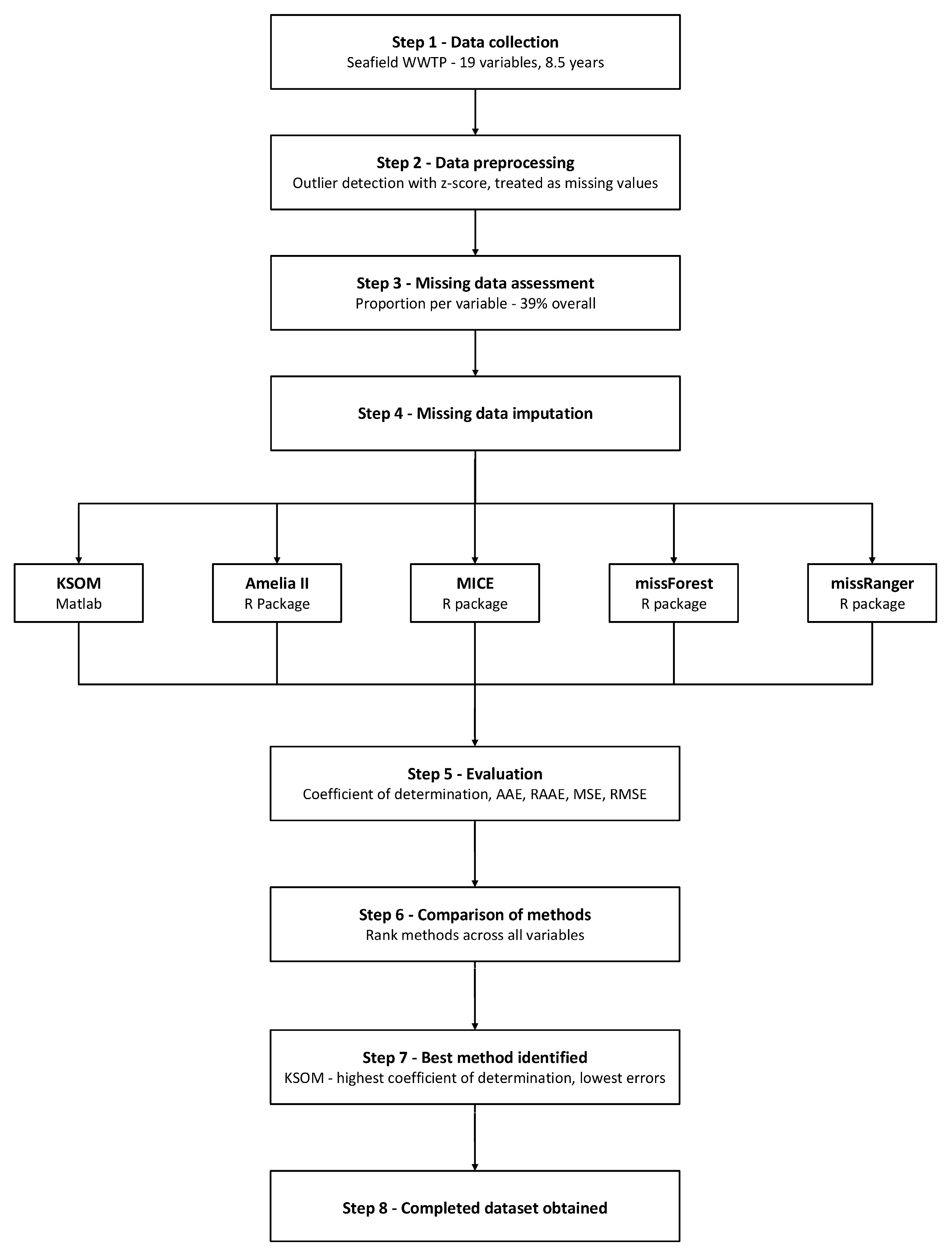
Figure 1. Methodology overview.
Waste 04 00017 g001
Figure 2. Map Layout of Seafield Treatment Plant—1 indicates screen house, 2 shows the detritors, 3 indicates grit washing, 4 shows sedimentation tanks, 5, 6, 7 show storm tank, aeration tank and final settling tank respectively, 8 indicates UV treatment, and 9 the outfall tunnel [27].
Waste 04 00017 g002
Figure 3. Illustration of Amelia’s process. Question marks indicate missing values in the dataset which is then bootstrapped into multiple versions before using the EM algorithm.
Waste 04 00017 g003
Figure 4. Illustration of the MICE algorithm process.
Waste 04 00017 g004
Figure 5. Illustration of the missForest algorithm. Question marks indicate missing values, orange squares indicate the missing values are classified as ‘predicted’, and green squares show the filled in missing values after prediction.
Waste 04 00017 g005
Figure 6. Illustration of the MissRanger algorithm. Question marks indicate missing values, orange squares indicate the missing values are classified as ‘predicted’, and green squares show the filled in missing values after prediction.
Waste 04 00017 g006
Figure 7. Illustration of Kohonen Self-Organising Maps process (orange colored node indicates the winning node and the nodes in peach color indicate neighbouring nodes).
Waste 04 00017 g007
Figure 8. Illustration of Best Matching Unit (BMU) process in Kohonen Self-Organising Maps algorithm—Red question marks indicate missing values and green X’s indicate predicted values using BMUs.
Waste 04 00017 g008
Figure 9. Component planes of KSOM.
Waste 04 00017 g009
Figure 10. Scatter plots for KSOM Method. (a) Measured vs. Predicted Influent (b) Measured vs. Predicted PS Settled Sewage (c) Measured vs. Predicted RL Flow (d) Measured vs. Predicted RL SS (e) Measured vs. Predicted RL Load (f) Measured vs. Predicted Biomass (g) Measured vs. Predicted Food (h) Measured vs. Predicted F/M Ratio (i) Measured vs. predicted Sludge Age (j) Measured vs. Predicted MLSS (k) Measured vs. Predicted MLSS SSVI (l) Measured vs. Predicted RAS SSVI (m) Measured vs. Predicted SSVI 3500 (n) Measured vs. predicted SAS Volume (o) Measured vs. Predicted RAS Volume (p) Measured vs. Predicted RAS SS (q) Measured vs. Predicted Effluent Flow (r) Measured vs. Predicted Effluent SS (s) Measured vs. Predicted Effluent COD.
Waste 04 00017 g010
Figure 11. Time series plots for Influent and Final effluent COD (KSOM imputation).
Waste 04 00017 g011
Figure 12. Time series plots for MLSS and Food (KSOM imputation).
Waste 04 00017 g012
Table 1. Comparison of imputation methods reviewed.
Imputation
Approach
The Method Introduced by the AuthorsSpecifics of Each Approach
Amelia II James Honaker, Gary King, Matthew BlackwellAssumes values are missing at random (MAR), imputes data using means and covariances in a bootstrap-based Expectation Maximization (EM) algorithm, and uses a joint modelling approach based on multivariate normal distribution [31].
MICEStef van Buuren, Karin Groothuis-OudshoornAssumes values are missing at random (MAR) and imputes data using PMM (Predictive Mean Matching) on a variable-by-variable (univariate) basis. It can be applied to any type of missing data, but it performs better when data are missing at random [18].
MissForestDaniel J. Stekhoven, Peter BühlmannNon-parametric imputation—can handle mixed-type data and nonlinear data structures. Applies a univariate Fully Conditional Specification (FCS) strategy [19].
MissRangerDaniel J. Stekhoven, Peter BühlmannMultiple Imputation variation of missForest. The addition of PMM (Predictive Mean Matching) ensures that imputed values are only those already seen in the data to avoid outliers [19].
KSOMTeuvo KohonenConverts input data into a 2D grid by clustering similar input patterns together and then compares features of the missing input vector to the closest matching features in the clusters to impute missing data [32].
Table 2. Software version and hyperparameters used for each imputation method.
Imputation
Approach
Software UsedSoftware VersionHyperparameters
KSOMMATLAB (SOM Toolbox)Matlab R2024aMap size: 22 × 13 (286 neurons), learning rate = 0.5, max iterations = 200
Amelia IIR package Amelia IIR 4.1.0 (RStudio)Max no. of imputations: m = 1
MICER package miceR 4.1.0 (RStudio)m = 10, iterations = 5, method = PMM
MissForestR package missForestR 4.1.0 (RStudio)ntree = 10, maxiter = 1, mtry = p/3
MissRangerR package missRangerR 4.1.0 (RStudio)ntree = 500, maxiter = 10, PMM donors (pmm.k) = 10
KSOM was implemented using the SOM Toolbox in MATLAB (MATLAB R2024a). Batch training was employed, as it is computationally more efficient than sequential training and typically results in lower quantization and topographic errors [27]. Initial training parameters, including learning rate and neighborhood radius, were set to default values recommended by the SOM toolbox. Based on analysis of the case study data, a map size of 22 × 13 (286 neurons) was selected. The final quantization error and topographic error were found to be 1.344 and 0.175, respectively.
Table 3. Number of Outliers identified using Z-score and modified Z-score.
VariablesZ-ScoreModified Z-Score
Influent to ASP1950
PS Settled Sewage SS2323
RL Flow2432
RL SS 1448
RL Load 1233
Biomass 115
Food 947
F/M3265
Sludge age369
MLSS1510
ML SSVI 32298
RAS SSVI 63
SSVI 3500125
SAS Volume 00
RAS Volume 00
RAS SS 1412
Final effluent flow66
Final effluent SS3827
Final effluent COD155
Table 4. Results from the Linear Regression model.
Evaluation MetricValue
R20.492
AAE9.95
RAAE0.12
MAE9.95
MSE177.26
RMSE13.31
Table 5. Coefficient of determination (R2) for the methods used.
VariableKSOMAmelia IIMICEMissForestMissRanger
Influent to ASP0.86970.19950.19940.19930.1985
PS Settled sewage SS0.63370.45470.43120.48590.5013
RL flow0.66290.16440.18540.28650.2891
RL SS0.92530.04510.01520.13120.2557
RL load0.90450.04360.01810.10840.2162
Biomass0.85320.44280.42450.57090.5846
Food0.84040.36840.40230.52630.4306
F/M0.87970.36250.4020.50720.452
Sludge age0.69240.01430.00910.01030.0111
MLSS0.77150.41620.3970.48120.5494
ML SSVI0.98540.56160.44950.73740.731
RAS SSVI0.83410.4860.48350.5840.6358
SSVI 35000.80080.45880.48090.56670.6148
SAS volume0.93820.38470.35450.55450.5739
RAS volume0.98520.03540.00610.06570.0488
RAS SS0.51490.16110.1650.22470.232
Final eff flow0.89720.17760.16980.41260.403
Final eff SS0.57520.42870.43370.44460.44
Final eff COD0.69040.32280.29470.39370.4452
Disclaimer/Publisher’s Note: The statements, opinions and data contained in all publications are solely those of the individual author(s) and contributor(s) and not of MDPI and/or the editor(s). MDPI and/or the editor(s) disclaim responsibility for any injury to people or property resulting from any ideas, methods, instructions or products referred to in the content.