Systemic Risk and Bank Networks: A Use of Knowledge Graph with ChatGPT

Abstract

In this paper, we study the networks of financial institutions using textual data (i.e., news). We draw knowledge graphs after the textual data has been processed via various natural language processing and embedding methods, including use of the most recent version of ChatGPT (via OpenAI api). Our final graphs represent bank networks and further shed light on the systemic risk of the financial institutions. Financial news reflects live how financial institutions are connected, via graphs which provide information on conditional dependencies among the financial institutions. Our results show that in the year 2016, the chosen 22 top U.S. financial firms are not closely connected and, hence, present no systemic risk.

1. Introduction and Related Work

In an increasingly interconnected financial world, understanding the intricate relationships between banks is critical to assess systemic risks and market dynamics. This paper aims to analyze the financial news from 2016 that embeds information of how financial firms are interrelated, by combining natural language processing (NLP) and large language models (LLMs) to deeply explore the interdependence of the banking industry.

The stability and resilience of the banking sector are critical to the global economy. Identifying and understanding the interdependencies among financial institutions is critical for effective risk management and regulatory oversight. Recent advances in natural language processing (NLP) and large language models (LLMs) provide us with unprecedented opportunities to extract valuable insights from large amounts of text data. To the best of our knowledge, this paper is the first one to utilize news data to quantify the interconnection of banks and provide a new angle of systemic risk measure. Specifically, using financial news from 2016, we create an extended knowledge graph that provides a deeper understanding of financial firm interdependencies.

Recently, Chen and Zhang [1] (2use knowledge graphs (KGs) to study the systemic risk of the banking industry. While there have been a large number of studies on banks’ networks, their work using KGs is the first. Knowledge graphs provide a graphical representation of the connections between entities (called vertices or nodes), with the strength of the connection reflected by the lines connecting them (called edges) or the distance between them. Therefore, knowledge graphs are a natural tool for visualizing relationships among financial institutions (Additionally, different data and diagram selections can demonstrate how entities are connected differently). KGs can be viewed as a non-parametric methodology, while the existing literature adopts a parametric (commonly Gaussian framework) setting. Our paper piggybacks on Chen and Zhang, by extending the data usage from numeral to textual data. In particular, we leverage upon recent technological advances in textual analysis such as Google’s Transformer, which can accurately interpret similarities of words and sentences.

The origin of knowledge graphs comes from graph theory, created by Leonhard Euler in 1735 when he solved the seven bridge problem in Königsberg (now Kaliningrad). Since then, with Euler’s development, related research has continued to expand. Very roughly speaking, there are four areas of development, as follows: probability graphic models (PGMs), knowledge graphs, directed graphs, and knowledge graph databases. In the first case, PGMs (Probabilistic Graphical Models) are similar to other network models such as Bayesian networks. Their basic concept is to express the multidimensional probability distribution of entities (describing how entities are connected) in a series of marginal and/or conditional probability distributions. This research direction focuses on estimating such networks and establishing statistical inferences. Therefore, usually, no chart needs to be presented. It is also worth noting that this line of research primarily assumes a Gaussian distribution for obvious mathematical considerations (hence, parametric). Due to its parametric nature, PGMs are more suitable for, for example, portfolio analysis (Denev [2]) and investor’s networks (Ozsoylev et al. [3] and Chung et al. [4]). This is different from the other cases that use non-parametric algorithms (i.e., machine learning).

Contrary to PGMs, in the second case (knowledge graphs, or KGs), graphs are essential in presenting the main results. Models (i.e., knowledge) are applied to create connections between entities of interest (such as stocks or banks). Depending on the purpose of the study, there are a number of different charts to choose from. Typically, “knowledge” is created using various machine learning models such as embedding and clustering methods. Text analysis (using NLP models) is also often used to create knowledge. KGs are more suitable for studying systemic risk, especially for the financial industry. This is because the way that financial institutions are connected to each other is quite complex. They hold each other’s assets and share common vulnerabilities to macroeconomic conditions. In addition, many large financial institutions are global, exposing them to various country risks. These complex connections across a broad and diverse range of risk factors (many not even numerical, such as political risk) make parametric studies of their connections quite difficult. Financial institutions, due to their specific interconnectedness, present a significant systemic risk, which was particularly evident during the 2008 crisis. Knowledge graphs that provide a network map are a tool that naturally presents the relationships between financial firms and are, therefore, very suitable for studying systemic risks.

Knowledge graphs are undirected graphs (i.e., edges have no directions). Directed graphs, on the contrary (i.e., edges are directional), are often used for studying causality. In particular, a directed acyclic graph, or DAG, allows us to make an immediate inference of causal (i.e., directional) relationships between two entities (vertices or nodes). Well-known tools in finance, such as Granger’s causality test and difference-in-difference test, are famous applications of DAGs.

In the last case, a knowledge graph is used to build a database. Such databases are crucial for search engines. In traditional databases, tables/columns (i.e., relational databases) are usually used and “keys” are used to connect various variables (i.e., “columns” in the table). However, in a knowledge graph database, an “adjacency matrix” is used to connect variables. This approach has revolutionized the way search engines like Google provide fast and relevant search results. Although PGMs (including network models) have been used in the financial field for quite some time, [ref] KGs are relatively new. This is because machine learning tools have only recently been introduced into finance.

This paper combines (as a modern trend) the following two areas of research: (1) banking and finance and (2) computer science. It is closely related to two lines of work in the literature, as follows: (1) banks’ systemic risk networks and (2) natural language processing (NLP) and large language models (LLMs).

We follow Chen and Zhang [1] and draw KGs of the top 22 US financial firms. Different from Chen and Zhang, our KGs are drawn on financial news, as opposed to distressed index or volatility, both of which are numeral data. Although the use of KGs to measure systemic risk is generally accepted, it remains a challenge as to which variables (features) to use. In a knowledge graph, relationships between any entities are measured as “edges”, where higher values indicate closer relationships and vice versa. As mentioned before, there are many options for variables to connect financial institutions, such as company fundamentals (e.g., liquidity, profitability, and credit risk), technical aspects (e.g., seasonality and momentum), management aspects (e.g., governance and strategies), and numerous other descriptive variables such as news, lawsuits, and analyst reports, among others. Ideally, all these variables should be incorporated into the network model to build a knowledge graph. Unfortunately, there is very limited work in the literature (Note that the existing literature almost entirely uses numeral data. Using returns is understandable because correlation is measured using returns. However, return is a composite indicator and, in many cases (such as systematic risk), is too broad and uninformative. There are some studies that do not use returns, including dissimilarity index (Boss et al. [5]), volatility (Ahelegbey [6]), stress index (Chen and Zhang [1] and Nicola et al. [7]), non-performing loans (Dolfin et al. [8]), and interest rates (Caccioli et al. [9])). In this paper, we aim to fill this gap by studying the interconnectedness of the top US financial firms using news data from 2016.

1.1. Systemic Risk and Banks’ Networks

Systemic risk generally refers to the failure (dysfunction) of financial systems, consequently causing economic recession. However, as emphasized by Ellis, Sharma, and Brzeszczyński [10], there is no widely accepted definition of systemic risk (Ellis, Sharma, and Brzeszczyński [10] summarized the definitions of systemic risk in the literature as follows: (1) the risk that an event will trigger a loss of economic value or confidence in a substantial portion of the financial system and have significant adverse effects on the real economy; (2) the failure of a significant part of financial institutions; (3) the risk that a national, or the global, financial system will break down; (4) an impairment of the financial system; (5) a correlation of defaults within the financial system over time; (6) a malfunctioning of the entire financial system; and (7) a loss of economic value or a widespread loss of confidence in the financial system). Thus, the assessment and measurement of systemic risk are important for policymakers and academics. For example, Billio et al. [11] regarded systemic risk as “… a series of correlated defaults among financial institutions, occurring over a short time span and triggering a withdrawal of liquidity…”; thus, they propose five measures of systemic risk (e.g., correlations and cross-autocorrelations) to demonstrate that four financial sectors had become highly interrelated before the global financial crisis of 2007–2009.

In general, there can be four sources of systemic risk (similar to our classification, Ellis, Sharma, and Brzeszczyński [10] review 60 systemic risk models in the literature and classifies them into the following five categories: (i) early warning and credit default swap indexes; (ii) credit and capital measure; (iii) liquidity measures; (iv) contagion measures; and (v) network measures). First, the systemic risk may be due to the contagion effect, e.g., one bank’s default may trigger the failure of other banks. For example, Benazzoli and Di Persio [12] argue that the default contagion can be spread over the whole network, in one of the following three different ways: (1) propagation due to a direct counterpart exposure, (2) propagation due to asset price contagion, and (3) propagation due to liquidity hoarding. Furthermore, Benazzoli and Di Persio [12] apply the Erdos–Renyi model, the Barabasi–Albert model, and a modification of the latter, to describe the random dynamics governed by financial failures and their related spread through the network.

Secondly, clearing mechanisms and the settlements of different transactions play an important role in the context of financial networks and systemic risk. They could affect the contract value and lead to observable liquidity problems, failed payments, losses, and insolvencies. For instance, Eisenberg and Noe [13] develop a clearing system model, which is consistent with the priority of debt claims and the limited liability of equity, and provide information on the systemic risk faced by the individual system firms. Rogers and Veraart [14] extend the work of Eisenberg and Noe [13] by considering the existence of extra costs in the clearing procedures and, under certain conditions, solvent banks may have motivations to rescue failing banks.

Thirdly, the cascades of bank defaults may be due to bilateral interbank exposures. For example, Gai and Kapadia [15] consider a financial network, in which financial intermediaries are randomly linked together by their claims on each other, and they show how losses can potentially spread via the complex network of direct counterparty exposures following an initial default (Hurd and Gleeson [16], Hurd [17], and Unicomb, Iniguez, and Karsai [18] had similar model settings and provided alternative approximation methods to compute the solution of cascade dynamics).

Finally, the financial distress may propagate between banks that hold common assets. For instance, Cifuentes, Ferrucci, and Shin [19] study the effect of losses due to common asset holdings and fire sales. They assume that banks are interacting through a network of interbank lending relationships and that all banks are investing in one common external asset. They find that there is a nonmonotonic relationship between the number of connections in the network and the number of observed defaults. Caccioli, Shrestha, Moore, and Farmer [20] and Caccioli, Farmer, Foti, and Rockmore [21] propose a model of overlapping portfolios, to examine the financial stability of the system in the limit when the number of banks and assets is large.

The literature that studies banks’ networks is voluminous. For example, recently, Anderson, Paddrik, and Wang [22] studied the amounts and locations of interbank deposits, thereby reshaping the bank networks. Dabrowski et al. [23] connect systemic banking crisis early warning systems with dynamic Bayesian networks. Using unique data on bank balance sheets and detailed interbank deposits from 1862 and 1867 in Pennsylvania, they quantify the effect on financial stability in an interbank network model. Gandy and Veraart [24] demonstrate how Bayesian networks can be used for financial firms. Anand, Craig, and Von-Peter [25] adopt interbank contagion to build a network of financial firms. Boss et al. [5] use network topology to study interbank connections in Austria. Elsinger, Lehar, and Summer [26] summarize recent network models and systemic risk assessment. They describe how simulations are designed and discuss the main insights that have been obtained using applications to the complex network of real-world exposure data of banking systems. Hałaj and Kok [27] assess interbank contagion using simulated networks. They present a new approach to randomly generate interbank networks with the availability to incorporate bank-by-bank bilateral exposures. Musmeci N. et. al. [28] reconstruct the global topological properties of a complex network, starting from limited information. They regard fitness as a non-topological quantity. Finally, Mastromatteo, Zarinelli, and Marsili [29] examine network tools such as maximum entropy to reconstruct credit networks for the risk of contagion by assuming a trivial (fully connected) topology, a type of network structure which can be very different from the one empirically observed.

1.2. Related Work to Banks’ Networks

As mentioned at the beginning of the introduction, networks are often represented as (undirected) graphs. As a result, they can directly be compared to knowledge graphs. Also from the literature review above, networks and probability graphic models (PGMs, discussed at the beginning of the introduction) are highly resemblant. As a result, the difference between network models and graphs is really just a matter of presentation.

Roughly speaking, one can view networks (or PGMs) as a parametric approach and knowledge graphs as a non-parametric approach. The advantage of knowledge graphs, due to their non-parametric nature, can be easily used in conjunction with textual data. This is the main contribution of this paper.

The literature reviewed above on systemic risk and banks’ networks all use numerical data from the government, such as financial market and financial reports, equity prices, credit default swap premiums, interest rate/bond yields, macroeconomic variables, foreign exchange rates, various real estate indices, and credit ratings (Although credit ratings are alphabetical, researchers convert them into numerical values (e.g., 1~9)). To the best of our knowledge, our paper is the first one to utilize news (textual) data to quantify the interconnection of banks and provide a new angle of systemic risk measures.

Among the network measures of the systemic risk literature, our paper is closely related to the word of Chen [30], because he also used a network model to study the relation between financial stability and interconnectedness among banks. Chen [30] assumed that banks form a financial network by swapping investment projects with other banks. Under this assumption, banks’ capital levels are contingent on the interconnectedness of the network and the financial stability can be inferred from the model. Although Chen’s [30] model is theoretically appealing, it is difficult to empirically test the model, because full information of banks’ investment projects and capital structure are required in order to estimate the model parameters. In complement to Chen [30], this paper empirically estimates the interconnectedness among banks, using financial news data.

Our paper is also closely related to the work of Chen and Zhang [1]. Recently, Chen and Zhang [1] used knowledge graphs (KGs) to study the systemic risk of the banking industry. The data they use are volatility and liquidity indexes. Our paper piggybacks on the work of Chen and Zhang by extending the data usage from numeral to textual data. We adopt their sample selection criteria, in an attempt to make our work parallel to theirs.

1.3. Related Work to NLP and LLMs

Our paper is also related to the stream of literature that uses textual data (e.g., financial news and twitter discussions) to extract the market or investor sentiment (mood) and study the prediction power of sentiment for future market movements. For example, Bollen, Mao, and Zeng [31] obtain public mood states from the text content of daily Twitter feeds, using two mood tracking tools, namely OpinionFinder that measures positive vs. negative mood and Google-Profile of Mood States (GPOMS) that measures mood in terms of six dimensions (calm, alert, sure, vital, kind, and happy). Their results suggest that the accuracy of DJIA predictions can be significantly improved by the inclusion of the calmness of the public, measured using GPOMS. In addition to social media text data such as Twitter, text mining for financial market predictions is widely studied, using various news data such as Bloomberg (Chatrath et al. [32]), Forbes (Rachlin, Last, Alberg, and Kandel [33]), Wall Street Journal (Antweiler and Frank [34]; Wong et al. [35]), Yahoo! Finance (Antweiler and Frank [34]; Schumaker et al. [36]), etc. The empirical results of these studies indicate that textual data are useful for predicting future movements of equity prices.

Regarding NLP, there has been a large amount of effort to use NLP in various areas in the financial world. The earliest adoption can be traced back to the early 2000s (see Fisher, Garnsey, and Hughes [37] for an excellent review). For example, Sydserff [38] uses a texture index for evaluating accounting narratives, while Back et. al. [39] compare numerical data and text information from annual reports. Since then, the use of textual analysis has been exploding. This paper joins this trend to use NLP on banks’ systemic risk networks. There are two new innovative contributions of our paper. First, we extend the use of NLP to LLMs, since LLMs employ the most advanced text-embedding technology. Secondly, we combine NLP–LLMs with knowledge graphs, to generate networks of banks, crucially needed information by regulators and practitioners. In the past, knowledge graphs have been mainly retrieved from numeral data (as mentioned above). Our paper adds to the literature by studying whether textual data (i.e., news) can provide a better insight.

2. Knowledge Graphs

A knowledge graph (KG) is a graph which displays (usually in a two-dimensional diagram) how each node (vertex) is connected with other nodes. The line connecting two nodes is known as an edge, whose value represents how close the two nodes are related (a higher value represents a closer relationship). The main advantage of KGs is their visualization. It allows the users to see visually how each node is connected to other nodes. Figure 1 is an example taken from a blog of neo4j, which is a popular KG database (By Tomaz Bratanic in https://neo4j.com/developer-blog/turn-a-harry-potter-book-into-a-knowledge-graph/ accessed on 1 March 2024). In Figure 1, all the characters in J.K. Rowling’s first four Harry Potter books are displayed in a graph. Each character is a node (vertex) and each line is an edge. The size of the bubble of each node represents how important a character is, while the distance between any two nodes measures how close the relationship is. It is obvious that Harry Potter is the most important character in the four-book series and is, therefore, placed in the center of the graph (hence, it is to be noted that the coordinates (i.e., x-y axis) in the graph carry no meaning in Figure 1, which is not necessarily so in other KGs).

By its name, a KG must contain “knowledge”. Knowledge is simply a model that creates the connections. In Figure 1, the knowledge used is all the texts in the first four Harry Potter books. By going through the entire four books, the connection of any two characters (e.g., Hermione Granger and Ron Weasley) is determined by how many times they are mentioned together. This requires the use of models in NLP (natural language processing) (For example, the author uses co-reference resolution, which replaces the pronouns with the referenced entities. Here, knowledge graph embedding is used. It is a technique used in natural language processing and machine learning to represent entities and relations in a knowledge graph as low-dimensional vectors in a continuous vector space.

There are various ways to generate a KG. If the location (i.e., coordinates) on the graph matters (i.e., the axes have meaning—this is usually the case where dimension reduction techniques are applied and, hence, the axes represent the most important features (or linear combinations of all features, e.g., PCA)) (We use “feature” and “explanatory variable” interchangeably. PCA is shorthand for principal component analysis). Moreover, the distance between any two vertices represents the “closeness” of the two vertices. If the location has no meaning (i.e., vertices are randomly placed by the graphic software for the sake of a nice visual), then edges are drawn with different degrees of thickness—with a thicker edge representing a closer relationship. In such a case, various machine learning methods (such as LASSO, clustering, and K-means, among numerous others) can be used to gauge the “closeness” of the vertices. In such graphs, vertices are arranged optimally (That is, the chosen graphic software will place the vertices optimally for a nice visual. Figure 1 is a “spring graph”, in which the least connected vertices will be put at the far sides of the graph and the Euclidian distance is not a good measure for closeness. In another example, the “graph” will place all vertices on the circumference of a circle (given that location has no meaning) and the closeness is entirely represented by the thicknesses of the edges) for visualization (i.e., closer vertices are more connected than farther vertices and, yet, where they are located in the x-y plane is not important).

As mentioned earlier, one can use various machine learning techniques to describe vertices and edges. These machine learning techniques may not be related, which provides a large amount of flexibility in building a KG. This is drastically different from PGMs, which must obey a parametric structure.

In sum, there is no standard way to present a KG. Authors can choose any visualization, as numerous packages are available for selection. Apparently this raises issues such as robustness, stability (stationarity), and other statistical concerns. In the remainder of this section, we briefly describe directed and undirected graphs, which are mostly concerned with PGMs (a standard KG is usually an undirected graph) and Gaussian PGMs, which is the most popular PGM. These are all parametric (or semi-parametric) models and are not directly related to this paper.

2.1. Directed and Undirected Graphs

As the names suggest, a directed or undirected graph is used to present a relationship in a symmetrical (latter) or asymmetrical (former) way. Typical examples in finance are joint defaults (former) and return correlations (latter). In the studies of joint defaults, conditional probabilities are used to describe the dependencies between two companies. For example, company A’s defaults may lead to the default of company B, but not vice versa. In such situations, a directed graph can be more suitable. On the other hand, return correlations are symmetrical and, hence, an undirected graph is more suitable.

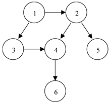
Directed graphs can be modeled via a series of conditional probabilities. The following graph depicts the basic idea of a directed graph:

• where arrows demonstrate dependencies. For example, node #1 depends upon nodes #3 and #0, but it is depended upon by nodes #2 and #4.

The joint probability of all six nodes can be shown, as a demonstration, as follows:

$$p(x_1,\cdots ,x_6)=p(x_1)p(x_2|x_1)p(x_3|x_1)p(x_4|x_2,x_3)p(x_5|x_2)p(x_6|x_4)$$

(1)

To reflect the dependencies, in this example, vertex 2 and vertex 3 are independent and conditional on vertex 1, usually labeled as $x_2\perp x_3|x_1$.

In general, a set of vertices have a joint probability, as follows:

$$p(x_1,\cdots ,x_n)={\displaystyle {\prod }_{i=1}^n}p(x_i|x_{\mathrm{Pa}(i)})$$

(2)

where $\mathrm{Pa}(i)$ represents the parents of $i$, as shown in the graph (and $i$ represents a vertex). For example, $\mathrm{Pa}(4)=\{2,3\}$, $\mathrm{Pa}(2)=\left\{1\right\}$, and $\mathrm{Pa}(1)=\varphi$. The random variable $x_A=(x_i:i\in A)$. Hence, if $A=\{2,3\}$, then $x_A=(x_2,x_3)$. Let $A=\mathrm{Pa}(4)=\{2,3\}$ and then $x_{Pa(4)}=(x_2,x_3)$.

Undirected graphs, also known as random fields, are depicted, as an example, as follows:

Take the usual notation of a graph, $G=\{V,E\}$, where $V$ contains all the vertices and $E$ contains all the edges. A complete graph is a graph in which every pair of vertices is adjacent. A complete subgraph of a graph will be called a clique. Hence, a clique, $C_X$, of a graph, $G$, is defined as a set of vertices, $X\subset V$, with the property that every pair of distinct vertices are adjacent. The maximal clique of a graph, $G$, is a clique such that there is no clique, $C_Y$, that contains all the vertices in $X$ and at least one other vertex.

As a result, the joint probability distribution can be written as follows:

$$p(x_1,\cdots ,x_n)=\frac{1}{Z}{\displaystyle \prod _{C\in \mathcal{C}(G)}}{\psi }_C(x_C)$$

(3)

where $\mathcal{C}(G)$ is the set of all cliques and $Z={\displaystyle \sum _{x_1\cdots x_n}}{\displaystyle \prod _{C\in \mathcal{C}(G)}}{\psi }_C(x_C)$ is a normalizer.

Hence, we can think of cliques as being independent marginal distributions. In the above graph, there is only one clique, which is the triangle of nodes #2, #4, and #5. Hence, the equation can be written as follows:

$$p(x_1,\cdots ,x_6)=p(x_2,x_4,x_5)p(x_1,x_2)p(x_1,x_3)p(x_3,x_4)p(x_4,x_6)$$

(4)

Clearly, in an undirected graph, relationships/dependencies are symmetrical. As mentioned earlier, the edges can be presented with different degrees of thickness (for a better visual). The edges can be estimated parametrically (e.g., using a Gaussian graphic model) or via machine learning methods (e.g., graphic LASSO) (Often, edges are modeled as partial correlation (inverse of the covariance matrix or precision matrix) or any definition of “distance”).

2.2. Banks’ Networks

As we can see, graphs (directed or undirected) are an ideal tool to identify networks of entities. Networks of banks are of particular interest, in that banks inherit a special risk that no other industry does. This is because banks hold each other’s assets and once one bank falls, it is likely to cause a bank run. This is known as the systemic (not systematic) risk.

Graphs can be drawn using either numeral data or textual data. Up till now, research on banks’ networks has been primarily focused on numeral data (returns, volatility, and distress indicators, among others). Such data provide substantial insight into banks’ networks, as their performances and risks are tied closely together. However, these numerical values are often reflections (i.e., result), not sources, of their interconnectedness. The sources (that they cross-hold assets) can show early signs of a problem via news and investigative reports.

Hence, in this paper, we use news data to investigate banks’ networks. To do so, we must adopt two key pieces of technology in processing news. The first is NLP, or natural language processing. In NLP, various text-embedding tools are available and we use Google’s word2vec and OpenAI’s text-embedding tool. The second is Attention, which is based upon similarity scores. We first build our own similarity scores and also use OpenAI’s Transformer.

3. Textual Analysis

From its name, it is clear that a textual analysis is a computer software used to analyze and further summarize texts and then present the results in a human-understandable manner. To achieve this goal, one must first ask oneself what texts (news, chats, and blogs, among other types) are the input and what forms are the output, such as graphs (for networks), indicators (like sentiment indexes to evaluate investment potentials), and clusters (for grouping), among many others. In each input–output pair, certain software can be identified as the most efficient. In presenting the result as a graph, dimension-reduction is necessary (as graphs are only visualizable in a two- or three-dimensional plot)—known as embedding. Various embedding methods are available and making the right choice is essential to the success of the textual analysis.

3.1. Natural Language Processing

Natural language processing, or NLP, has a wide variety of applications, from textual analysis to voice recognition. It involves a set of techniques that are related to computer science knowledge, such as tokenization, stemming and lemmatization, and word embeddings, to name a few.

3.1.1. word2vec

word2vec is a technique in natural language processing (NLP) for obtaining vector representations of words. These vectors capture information about the meaning of the word and their usage in context. The word2vec algorithm estimates these representations by modeling text in a large corpus.

doc2vec is an extension of the word2vec model, representing words in continuous vector space. doc2vec is a neural network-based approach that learns the distributed representation of documents. It is an unsupervised learning technique that maps each document to a fixed-length vector in a high-dimensional space. The vectors are learned in such a way that similar documents are mapped to nearby points in the vector space. This enables us to compare documents based on their vector representation and to perform tasks such as document classification, clustering, and similarity analysis.

There are two main variants of the doc2vec approach, as follows: (see https://www.geeksforgeeks.org/doc2vec-in-nlp/, accessed on 1 March 2024, for a short description)

• Distributed Memory (DM)
• Distributed Bag of Words (DBOWs)

The basic idea behind Distributed Memory is to learn a fixed-length vector representation for each piece of text data (such as a sentence, paragraph, or document), by taking into account the context in which it appears. In the DM architecture, the neural network takes two types of inputs—the context words and a unique document ID. The context words are used to predict a target word and the document ID is used to capture the overall meaning of the document.

The network has two main components—the projection layer and the output layer. The projection layer is responsible for creating the word vectors and document vectors. For each word in the input sequence, a unique word vector is created, and for each document, a unique document vector is created. These vectors are learned through the training process, by optimizing a loss function that minimizes the difference between the predicted word and the actual target word. The output neural network takes the distributed representation of the context and predicts the target word.

DBOWs is a simpler version of the doc2vec algorithm that focuses on understanding how words are distributed in a text, rather than their meaning. This architecture is preferred when the goal is to analyze the structure of the text, rather than its content. In the DBOWs architecture, a unique vector representation is assigned to each document in the corpus, but there are no separate word vectors. Instead, the algorithm takes in a document and learns to predict the probability of each word in the document, given only the document vector.

The model does not take into account the order of the words in the document, treating the document as a collection, or “bag”, of words. This makes the DBOWs architecture faster to train than DM, but potentially less powerful in capturing the meaning of the documents.

doc2vec can capture the semantic meaning of entire documents or paragraphs, unlike traditional bag-of-words models that treat each word independently. It can be used to generate document embeddings, which can be used for a variety of downstream tasks such as document classification, clustering, and similarity search.

doc2vec can handle unseen words by leveraging the context in which they appear in the document corpus, unlike methods such as TF-IDF (short for term-frequency and inverse-document-frequency) that rely on word frequency in the corpus. It can be trained on large corpora using parallel processing, making it scalable to big data applications. It is flexible and can be easily customized by adjusting various hyperparameters such as the dimensionality of the document embeddings, the number of training epochs, and the training algorithm.

3.1.2. spaCy

spaCy is an open-source software library for advanced natural language processing, written in the programming languages Python and Cython (see https://www.freecodecamp.org/news/getting-started-with-nlp-using-spacy/ accessed on 1 March 2024 for the key features of spaCy). The library is published under the MIT license and its main developers are Matthew Honnibal and Ines Montani, the founders of the software company Explosion.

Unlike NLTK (natural language toolkit) (see https://www.nltk.org/ accessed on 1 March 2024 for its documents), which is widely used for teaching and research, spaCy focuses on providing software for production usage. spaCy also supports deep learning workflows that allow for the connection of statistical models trained by popular machine learning libraries like TensorFlow, PyTorch, or MXNet, through its own machine learning library, thinc (see https://pypi.org/project/thinc/ accessed on 1 March 2024 for its documents). Using Thinc as its backend, spaCy features convolutional neural network models for part-of-speech tagging, dependency parsing, text categorization, and named entity recognition (NER). Prebuilt statistical neural network models to perform these tasks are available for 23 languages, including English, Portuguese, Spanish, Russian, and Chinese, and there is also a multi-language NER model. Additional support for tokenization for more than 65 languages allows users to train custom models on their own datasets as well.

spaCy provides a wide range of pre-trained models that can quickly analyze text and extract various linguistic features. These features include part-of-speech tags, named entities, syntactic dependencies, sentence boundaries, and more. The pre-trained models are trained on large corpora and have high accuracy, allowing developers to focus on their specific NLP tasks, without worrying about training models from scratch.

Tokenization is a crucial step in NLP that breaks down text into individual words or subwords. spaCy’s tokenization algorithms are highly efficient and language-specific, allowing for accurate and customizable tokenization. spaCy can also automatically segment text into sentences, making it easy to work with text data at a granular level.

Named entity recognition (NER) is the task of identifying and classifying named entities such as persons, organizations, locations, dates, and more. spaCy’s NER capabilities are exceptional, providing out-of-the-box support for multiple languages. It allows developers to train custom NER models using their own labeled data, enabling domain-specific entity recognition.

Dependency parsing involves analyzing the grammatical structure of a sentence by determining the relationships between words. spaCy’s dependency parsing is based on efficient algorithms and achieves high accuracy. It provides a rich set of syntactic annotations, including the head of each word, the dependency label, and the subtree structure. This information is invaluable for tasks like information extraction, question answering, and sentiment analysis.

One of spaCy’s major strengths is its flexibility and extensibility. Developers can easily customize and fine-tune spaCy’s models to adapt to specific domains or improve performance on specific tasks.

The library also provides a straightforward API for adding custom components, such as new tokenizers, entity recognizers, or syntactic parsers, making it a versatile tool for research and development.

spaCy is known for its exceptional performance and scalability. The library is implemented in Cython, a programming language that compiles Python-like code into highly efficient C/C++ modules. This allows spaCy to process text data blazingly fast, making it suitable for large-scale NLP applications and real-time systems.

3.2. Large Language Models

Large language models (LLMs), such as GPT-4, are artificial intelligence models that are trained based on large amounts of text data and are good at handling natural language processing tasks. The application of LLMs in the fields of document summarization, translation, keyword extraction, and document correlation analysis demonstrates its powerful language understanding and generation capabilities. The relationship between text embedding and large language models can be understood from the methods of data representation and natural language processing.

3.3. Embedding

In machine learning studies, it is customary to use a large amount of data with a large number of features. Given the complex nature of these (non-parametric) data and features, in many cases, features are not linearly related and need to be transformed in order to obtain accurate results. This is known as graph embedding. As a result, graph embedding is generally understood as a dimension reduction tool, to map a complex graph into a usually three- or two-dimensional drawing for easy visualization. It is well known that any finite graph can be embedded in three-dimensional Euclidean space and a planar graph is one that can be embedded in two-dimensional Euclidean space (for example, see Cohen [40], who provide fundamental mathematical results for three-dimensional graph drawing (embedding)).

Formally, the embedding of a graph, $G$, on a surface, $\mathsf{\Sigma }$, is a representation of $G$ on $\mathsf{\Sigma }$, in which points of $\mathsf{\Sigma }$ are associated vertices and arcs are associated with edges, in such a way that

• the endpoints of the arc associated with an edge, $e$, are the points associated with the end vertices of $e$,
• no arcs include points associated with other vertices, and
• two arcs never intersect at a point which is interior to either of the arcs.

3.3.1. Knowledge Graph Embedding

Knowledge graph embedding is a type of representation learning between entities and relations in a knowledge base. The entities and relations are mapped into a low-dimensional space, representing the semantic information between entities and relationships. We classify knowledge embedding into two broad areas. The first is unfolding. The most famous case is the Swiss roll example, where a roll is unfolded into a plane (see, for example, https://scikit-learn.org/stable/auto_examples/manifold/plot_swissroll.html, accessed on 1 March 2024). This includes isomap, locally linear embedding, spectral embedding, Hessian eigenmapping, local tangent space alignment, multi-dimensional scaling (MDS), and t-distributed stochastic neighbor embedding (t-SNE), among others.

The second is to investigate the relation of any two nodes using textual data, known as translation distance models. Both entities and relations can be represented as vectors in the same space. This includes DistMult, TransE, TransH, TransR, ComplEx, ConvE, and KG2E, among others. Note that these methods use textual data. These knowledge graph embedding methods aim to capture the semantic and structural information of entities and relations in knowledge graphs. These embeddings can then be used as features for various downstream tasks, such as knowledge graph completion, entity recommendation, and question answering.

Finally, we should note that graphs are often used, like other machine learning tools, to perform classification, clustering, regression, anomaly detection, and feature learning, among others. All of these tasks have their counterparts in network analysis. Researchers in network science have traditionally relied on user-defined heuristics to extract features from complex networks (e.g., degree statistics or kernel functions). However, recent years have seen a surge in approaches that automatically learn to encode network structure into low-dimensional embeddings, using techniques based on deep learning and nonlinear dimensionality reduction. These network representation learning (NRL) approaches remove the need for painstaking feature engineering and have led to state-of-the-art results in network-based tasks, such as node classification, node clustering, and link prediction.

3.3.2. Text Embedding

Text embedding is a technique for converting words, phrases, or entire paragraphs of text into numerical vectors. These vectors capture the semantic properties of words, such as meaning, contextual relevance, etc. Through text embedding, the model can mathematically process and analyze natural language. These embeddings are usually vectors in a high-dimensional space that can reflect the similarities and differences between different words. Text embedding is the basis for LLMs to process natural language. LLMs typically contain one or more layers within their internal architecture, specifically responsible for converting text into vector representations. When training an LLM, the model learns how to map words and sentences into an embedding space that can effectively express their semantic meaning. This enables the model to capture the nuances of language, allowing for a more accurate understanding and generation of natural language.

4. Empirical Results

We study the systemic risk of the financial sector in the year of 2016, using news data. The systemic risk is represented via a knowledge graph. The network presented in the knowledge graph demonstrates how the top financial firms are interconnected in the year of 2016.

4.1. Data

The data we use are the news data from LexisNexis. The data contain news of S&P500 firms in 2016, which are stored in an SQLite format. A snapshot of the sample is given in Figure 2. There are 296,584 news articles in total, covering 1324 organizations. The data are summarized in Panel (A) of

Table 1. Summary of data. (A) The entire sample; (B) top 22 financial firms.

(A) The entire sample:
Number of organizations	1324
Number of documents	296,584
Number of sentences	22,210,824
Number of words	236,338,448
Number of characters	1,677,880,582
(B) Top 22 financial firms:
Number of organizations	22
Number of documents	7031
Number of sentences	178,089
Number of words	4,886,736
Number of characters	27,637,528

.

Following Chen and Zhang [1], who studied the largest 25 financial firms in the U.S., we intend to construct a knowledge graph (KG) of the interdependencies among the same firms, with news data (The original firms adopted by Chen and Zhang [1] also include ACE LIMITED, TRUIST FINANCIAL CORP, and HEALTH CARE PROPERTY INVESTORS INC, but these firms do not have news in our dataset and, hence, cannot be included in our study). Out of the 25 firms adopted by Chen and Zhang, we could only identify 22 firms in our news dataset. They are presented in

Table 2. Top 22 financial firms.

Firm ID	Firm Name
0	AFLAC
1	AMERICAN EXPRESS
2	AMERICAN INTERNATIONAL GROUP
3	AMERICAN TOWER
4	BANK OF AMERICA
5	BANK OF NEW YORK MELLON
6	BERKSHIRE HATHAWAY
7	BLACKROCK
8	CAPITAL ONE FINANCIAL
9	CHUBB LTD
10	CITIGROUP
11	FRANKLIN RESOURCES
12	JPMORGAN CHASE
13	METLIFE
14	PNC FINANCIAL SVCS
15	PRUDENTIAL FINANCIAL
16	PUBLIC STORAGE
17	SIMON PROPERTY
18	STATE STREET
19	TRAVELERS COS
20	U S BANCORP
21	WELLS FARGO

Note: These top 22 financial firms are taken from Chen and Zhang [1]. They originally have 25 financial firms, but the news dataset we have only contains 22 out of those 25 financial firms.

. Now, the number of news articles reduces to 7031. The summary statistics are given in Panel (B) of Table 1.

We use NLP and LLMs to analyze the large amount of financial texts and extract refined insights about banking relationships.

4.2. Natural Language Processing

As introduced in the textual analysis section, we use doc2vec and spaCy to process textual data. These NLP methods perform text standardization, entity recognition, and semantic analysis to prepare data for further processing. Take the following news text as an example:

Indian Banking News 5 January 2016 Tuesday 6:30 AM EST JPMorgan Chase to Report Fourth-Quarter, Full-Year 2015 Financial Results on JPMorgan Chase’s Investor Relations Website LENGTH: 199 words Jan. 5—JPMorgan Chase & Co. (“JPMorgan Chase” or the “Firm”) will post its fourth-quarter and full-year 2015 financial results at approximately 6:45 AM EST on 14 January 2016 on the Firm’s Investor Relations website at jpmorganchase.com/latest-earnings. JPMorgan Chase will notify investors that earnings results have been issued through its social.

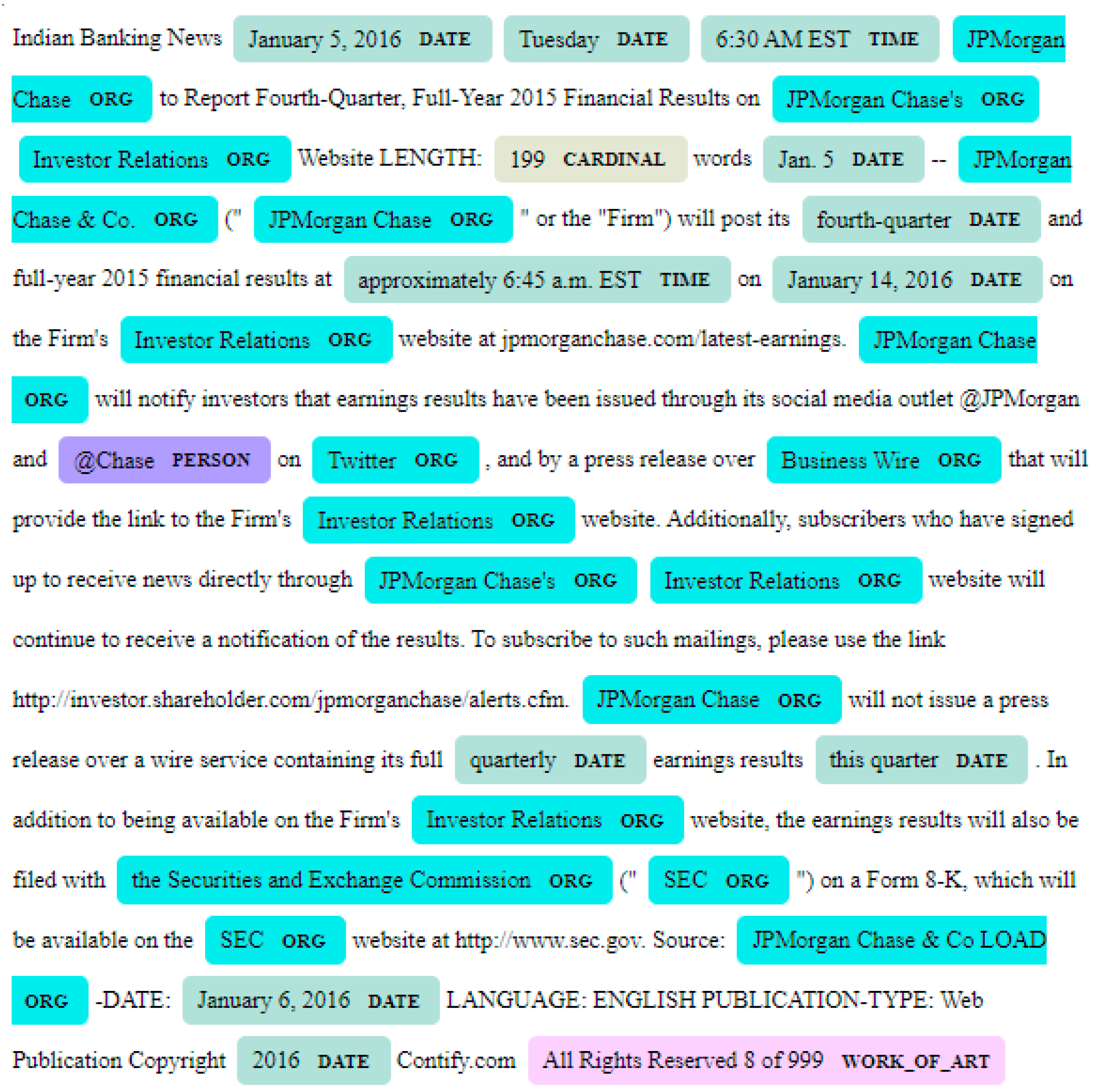
Using NLP/NER technology based on Python’s spaCy module, we can obtain the following NER-tagged text output. The NLP can process it to be the output as Figure 3:

Among them, the aqua highlighted terms are “ORG”, which means that the word is the name of “organization or company”. Similarly, purple is “PERSON”, light-purple is “WORK_OF_ART”, and light-green is “DATE” or “TIME”.

Using this type of information, we can further use traditional NLP techniques to find connections between documents and deduce dependencies between financial firms.

4.3. Embedding

Text embedding is a useful feature in many applications, such as semantic search and calculating text similarity. OpenAI’s text-embedding-ada-002 model is a digital representation of text that can measure the correlation between two pieces of text. This model is OpenAI’s second generation embedding model that is suitable for search, clustering, recommendation, anomaly detection, and classification tasks.

Embedding refers to converting the digital representation of an object or concept into a digital sequence (simply a vector), which enables computers to simply understand the relationship between objects and concepts. OpenAI’s text-embedding-ada-002 can handle longer contexts. Official documents indicate that the longest number of tokens in a text string can reach 8191. The resulting vector of each embedding is 1536 dimensions. This means that as long as the total length of the text is within 8191 tokens, this model will be converted into a fixed-dimensional normalized vector (dim = 1536). See Figure 4 for an exemplification.

The left box of Figure 4 is the original text. The middle box is OpenAI’s embedding, which results in the right box of a vector of 1536 numbers. The details of this embedding can be found in Neelakantan et al. [41].

Figure 5 presents a full example of a news piece. The text (top half of Panel (A) of Figure 5) we send to OpenAI, regardless of whether the total number of letters (seen in the nChars, or number of characters, column) in the lower half of Panel (A) of Figure 5) is 7280, 6725, or 14,410, OpenAI’s text-embedding-ada-002 model always returns an embedding (semantic) vector of dimension 1536.

But one thing that must be considered in detail is that OpenAI is a paid service. Using this embedding model, every 1 token = USD 10⁻⁷, so 10⁶ tokens = USD 0.1, and 10⁹ tokens = USD 100, which is probably still a small-scale service. This is an acceptable price range for the research project (OpenAI charge in terms of tokens, 1 token = 4.63 Chars, with std= 0.48).

4.4. Preliminary Investigation

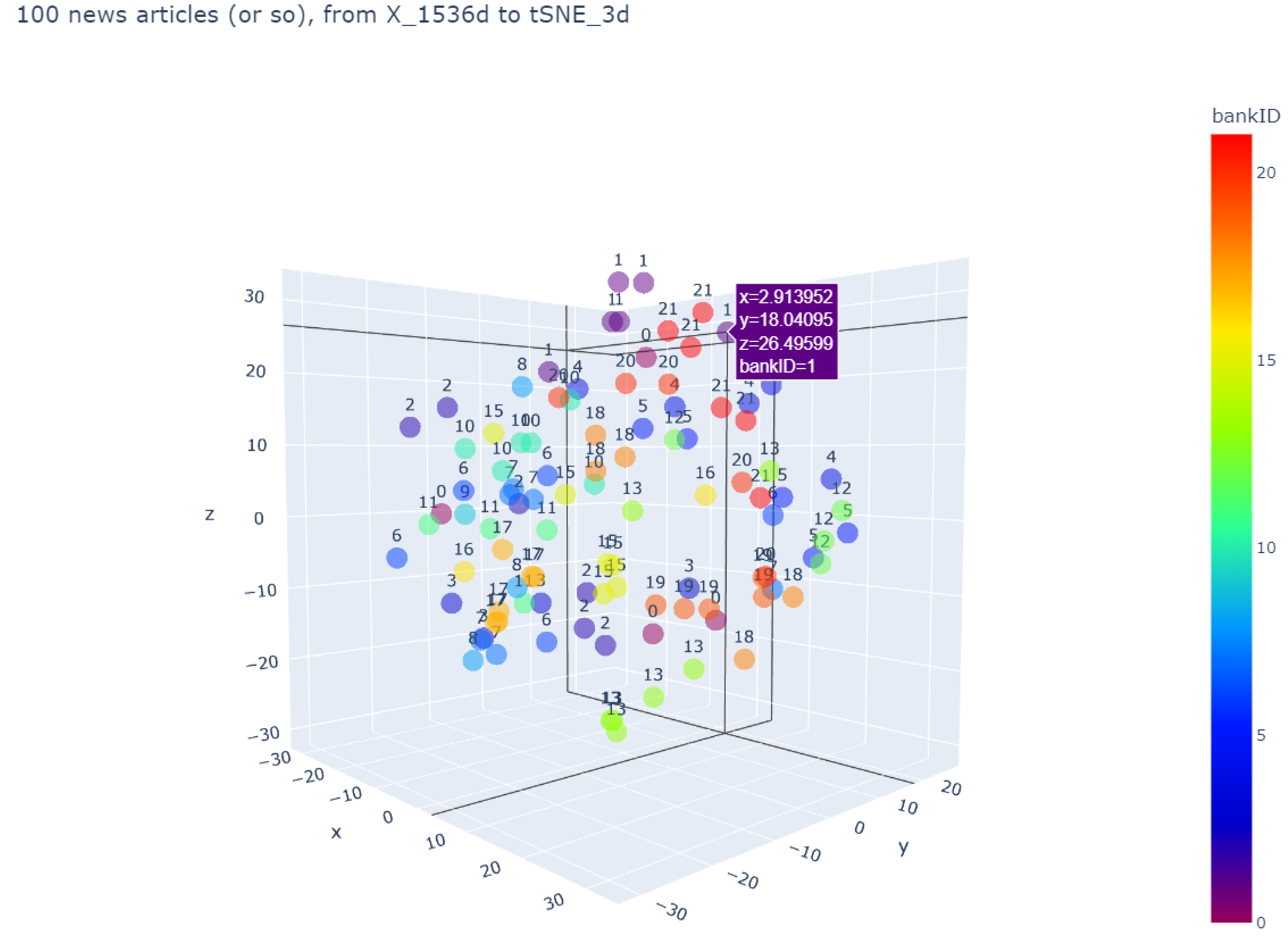
Our main goal is to draw a knowledge graph of the news data. The vertices are the 22 largest U.S. financial firms and the edges are estimated from the news data. We use OpenAI embedding to run every piece of news to a vector of 1536 numbers. Then, we convert the dim = 1536 vector to a dim = 3 vector, through a dimensionality reduction algorithm of PCA, LSA, or t-SNE. In Figure 6, we randomly sample 100 news articles (out of 7031) and plot them in a three-dimensional graph.

In Figure 6, each color represents a financial firm (and a number associated with it). Given that there are 100 articles and 22 financial firms, each financial firm will appear, on average, roughly five times. For example, on the top, there are two purple dots (associated with number #1), which is American Express. We can see that there are a total of five appearances of American Express, all close together at the top of the graph. Similarly, if embedding and dimension reduction models work properly, all the same-colored dots should be close together. From Figure 6, we can see that this is not the case for all financial firms. Aflac (number #0), for example, is scattered all over the space.

In Figure 6, each article in the dataset has a corresponding financial company. This is provided via an unknown choice from an NLP model. We can perform our own classification task of supervised machine learning accordingly, so that we can observe the embedding semantic discrimination ability provided by the dataset. Common classifiers we use include k-neighbors classifier, SVC, logistic regression, random forest classifier, XGB classifier, and MLP classifier, among others. Except for XGB, the rest can be obtained from the mainstream Python sk-learn module.

We divide the 7031 articles of the top 22 US financial firms into training sets and test sets (train-set vs. test-set), according to a 70%:30% ratio, and performed classification experiments (target categories = 22), the recognition rate results are listed as follows, where the number represents the classification accuracy, ranging from 0.00 to 1.00. The results are reported in

Table 3. Various training results.

Embedding	openAI-1536	openAI-1536	openAI, PCA-300	openAI, PCA-300	spaCy-300	spaCy-300
Data subset	train-set	test-set	train-set	test-set	train-set	test-set
Classifiers:
K-Neighbors Classifier	85.65%	79.00%	65.65%	46.68%	86.45%	79.19%
SVC	90.75%	84.45%	44.42%	40.52%	96.75%	86.30%
Logistic Regression	84.56%	82.70%	70.61%	65.21%	83.78%	82.56%
Random Forest Classifier	99.92%	79.29%	99.91%	53.83%	99.92%	80.81%
XGB Classifier	99.92%	82.23%	99.91%	58.90%	99.92%	82.13%
MLP Classifier	98.80%	86.87%	86.85%	71.32%	98.86%	84.93%

.

We observe that when using OpenAI’s original dim = 1536 (or 300) embedding vector, the best classifier is the MLP Classifier (Multi-layer Perceptron), with an accuracy ratio of 86.87%. However, if we use dimensionality reduction technology to reduce 1536 to 300 dimensions before performing the classification task, then the performance reduces significantly from 86.87% to 71.32%. In order to keep the benefits of smaller dimensionality, we test another text embedding scheme, the spaCy’s large language model, which also generates 300-dimensional vectors; then, the best classifier becomes SVC (support vector machine (classifier)), with an accuracy ratio of 86.30%. Here, the MLP Classifier still achieve a good accuracy of 84.93%, slightly worse than that in SVC.

It should be noted that each classifier has its own fine-tuning parameters (hyper-parameters). The above preliminary experiments do not include the fine-tuning of the hyper-parameters. The preset hyper-parameters in the sk-learn module are used to conduct experiments. This is the first step to select a classifier (not necessarily the best).

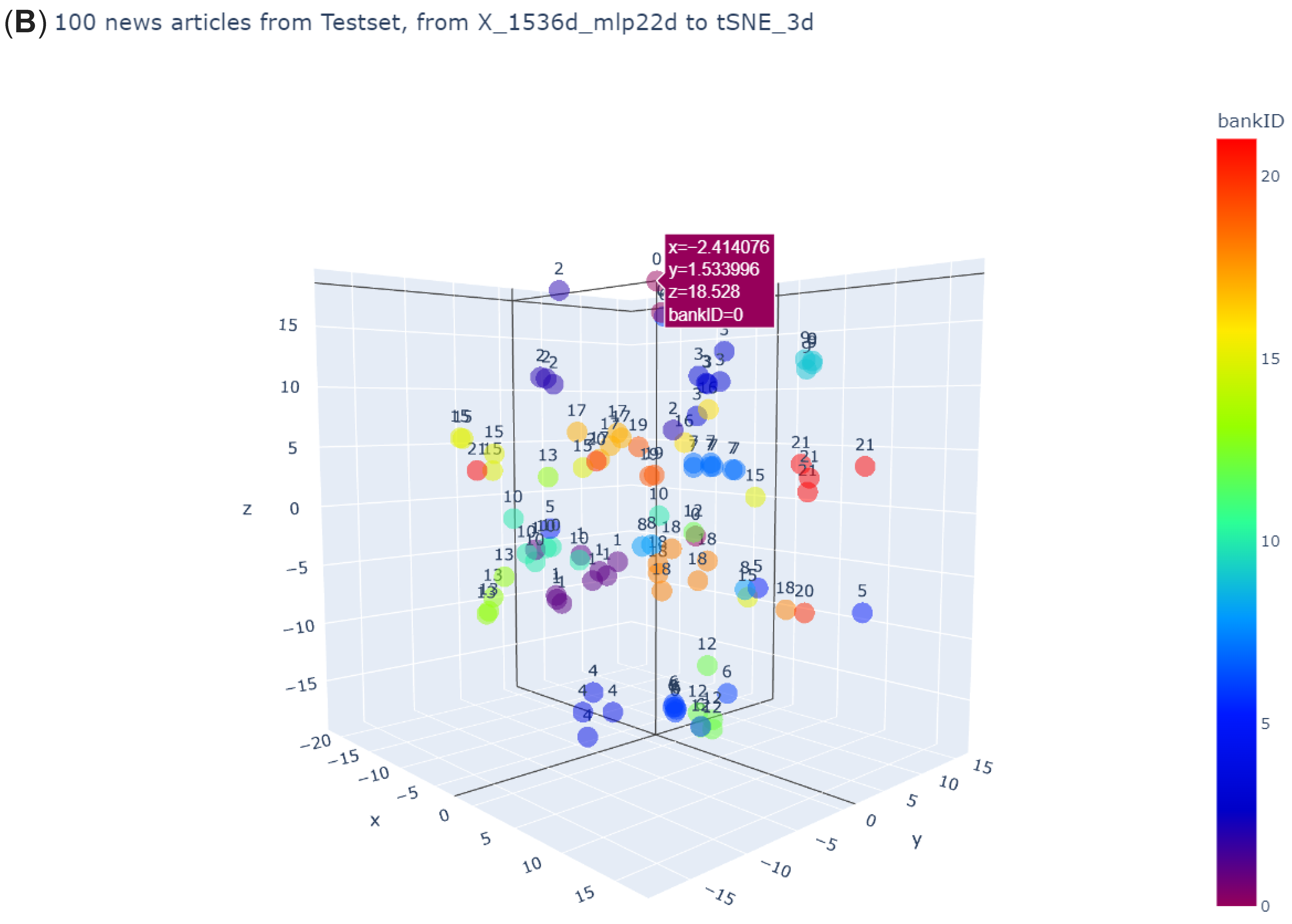
After the embedding vector of dim = 1536 is processed by the classifier, it becomes an output vector of dim = 22. Each dimension can exactly be regarded as the degree of association between the article and each of the 22 financial firms. If this output vector is close, one-step dimensionality reduction to dim = 2 or dim = 3 and projecting them onto a 2D plane (Panel (A) of Figure 7) or 3D space (Panel (B) of Figure 7) will present the visual effects of the following two pictures.

Comparing Panel (B) of Figure 7 and Figure 6, we can see the big difference. Now, the same-colored dots tend to stay close to one another. Yet, note that the 22 classifications do not represent any particular financial firm.

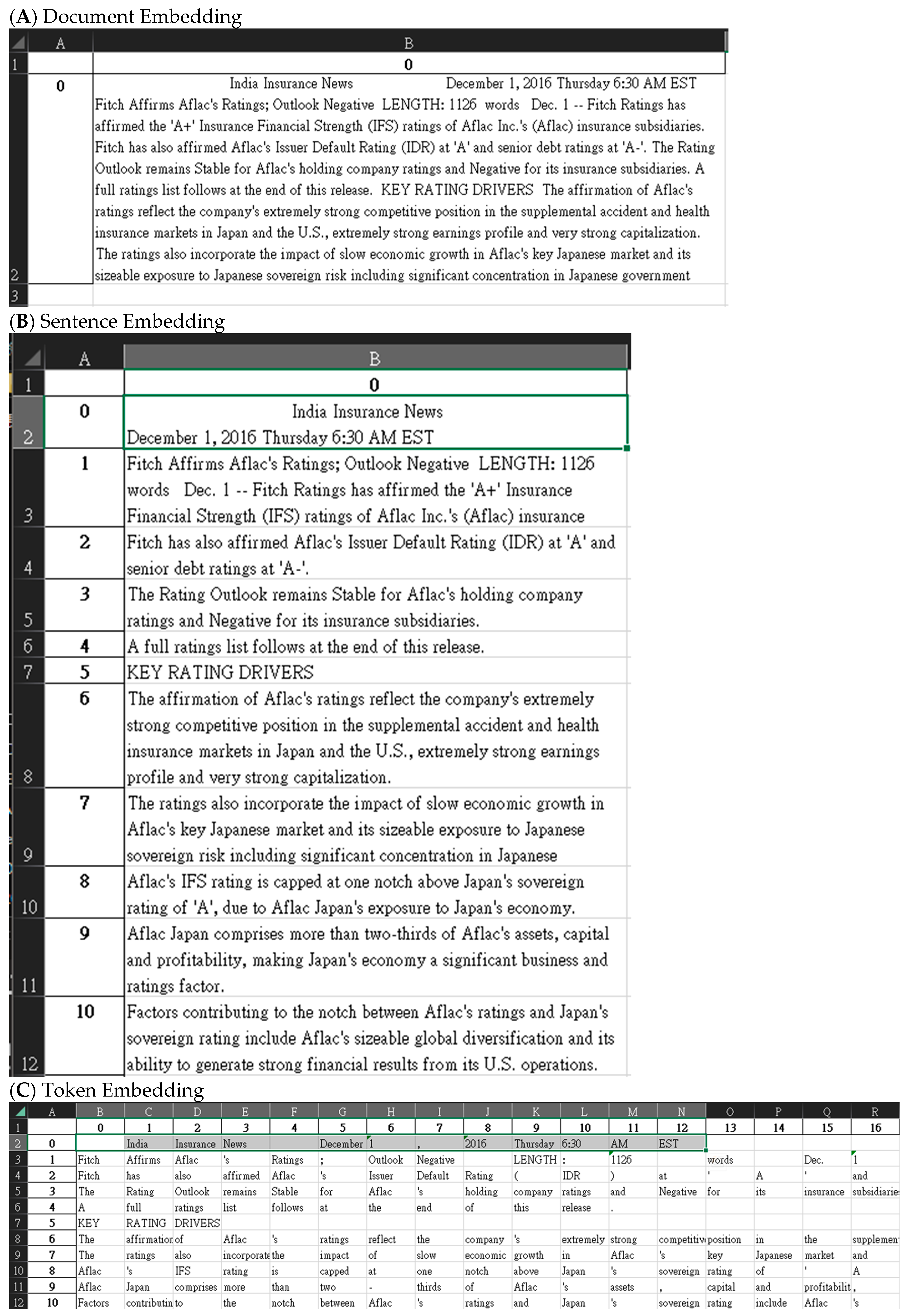
It is feasible to embed vectors with smaller language units than documents. For example, an article usually has a different number of sentences (sentences) and each sentence has a different number of words (words). Using sentences or words as embedding units is a research option that can be tried. What is more challenging is that the cluster classifier required for this fixed-dimensional but variable-length input vector “sequence” will become more complex. Advanced deep learning architectures such as CNN, RNN, LSTM, and Transformer will be further listed as research objects.

Phase 1: document-wise embedding, looking at the whole document as an entity and embedding it as a vector. This is demonstrated in Panel (A) of Figure 8.

Phase 2: sentence-wise embedding, dividing the whole document into many sentences, looking at each sentence as an entity, and embedding them as vectors to form a vector sequence. This is demonstrated in Panel (B) of Figure 8.

Phase 3: token-wise embedding, dividing the whole document into many sentences, then dividing the sentence into tokens, looking at each token as an entity, and embedding them as vectors to form a sequence of vector sequence, or 3D arrays, also called a 3D tensor. This is demonstrated in Panel (C) of Figure 8. Note that each cell in the following data table represents a vector (dim= 1536, in terms of OpenAI embedding).

4.5. Knowledge Graph

Finally, we draw knowledge graphs. The results presented in this sub-section are based upon a test sample (which is 30% of the total sample) and MLP Classifier (Multi-layer Perceptron Classifier, see Table 3).

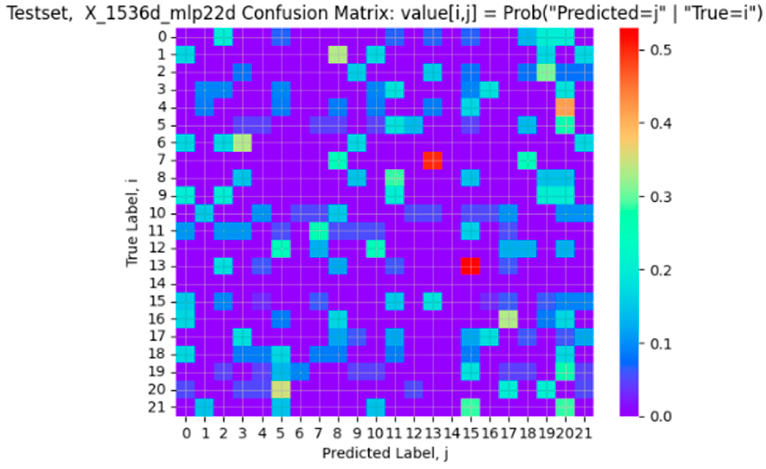
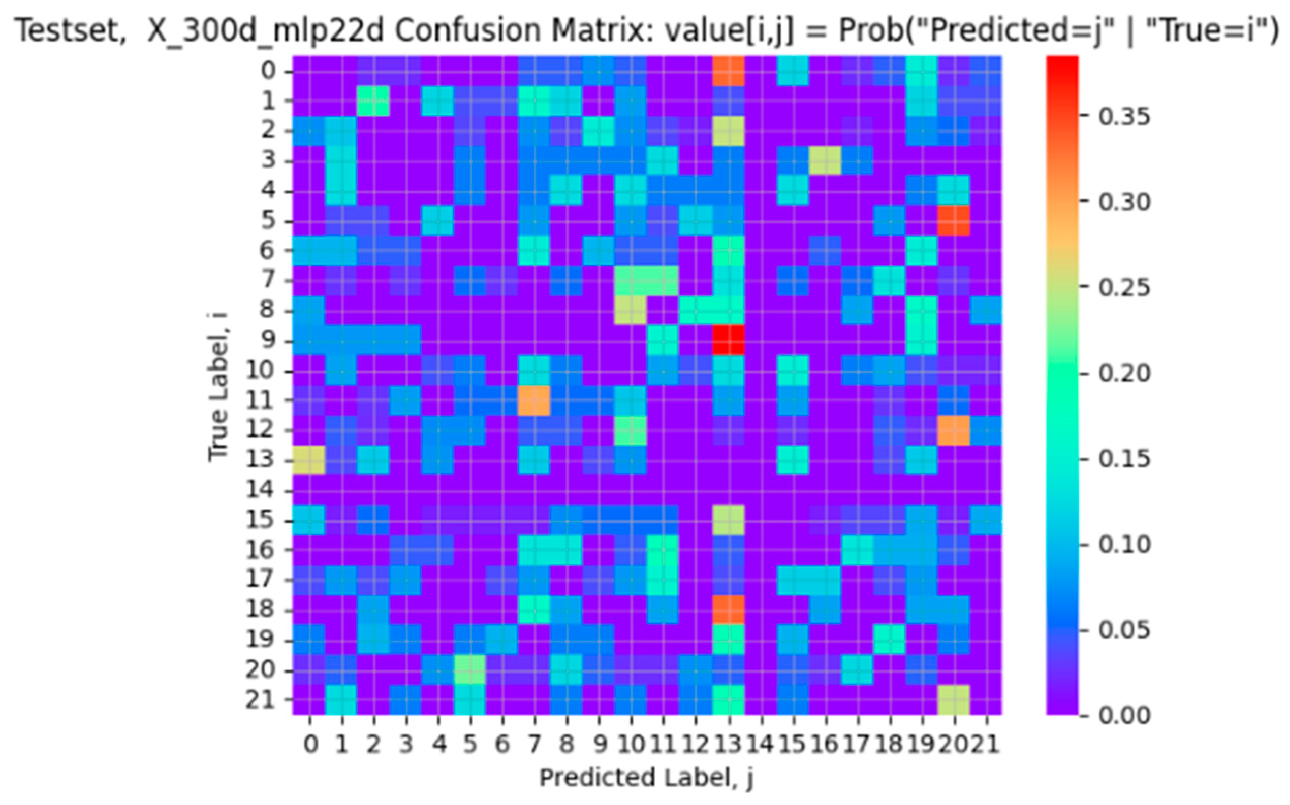
We use t-SNE to reduce the dimensionality to two. Then, we can use the confusion matrix in Python’s sk-learn module to create the heat map, as shown in Figure 9. The confusion matrix in Figure 9 is similar to those used in image processing. Each row contains a normalized set of weights (which sum to 1), except for itself. For example, for any given i-th row, except for the i-th column, every other column (say, the j-th column and j≠i) is a weight associated with row i. The highest weight of column j represents that firm j has the highest probability to be confused with firm i (hence, the so-named confusion matrix). In other words, firm j is the most closely related to firm i. This is similar to the concept of correlation, when numerical values are used. Given that we cannot calculate correlation using textual data, we adopt the confusion matrix instead.

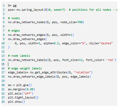
Finally, using Python’s networkX module, we can draw the graph. Here, we set each node in the graph as the name of the financial firm (or the associated number, as shown in Table 2) and the edge is the relationship between financial firms. In order for the easy visualization of the graph, the number of edges for any financial firm is limited to no more than three (see Figure 10). Note that the vertices are numbered according to Table 2.

It should be noted that firm #14 (PNC) is removed from the confusion matrix in Figure 9. This is because it has only one news item in the dataset, which generates a spurious relationship to firm #2 (AIG). Hence, the row for firm #14 is set to 0 for all columns. As a result of that, firm #14 has no relationship with any other firm. It is, hence, by itself in the knowledge graphs in Figure 10.

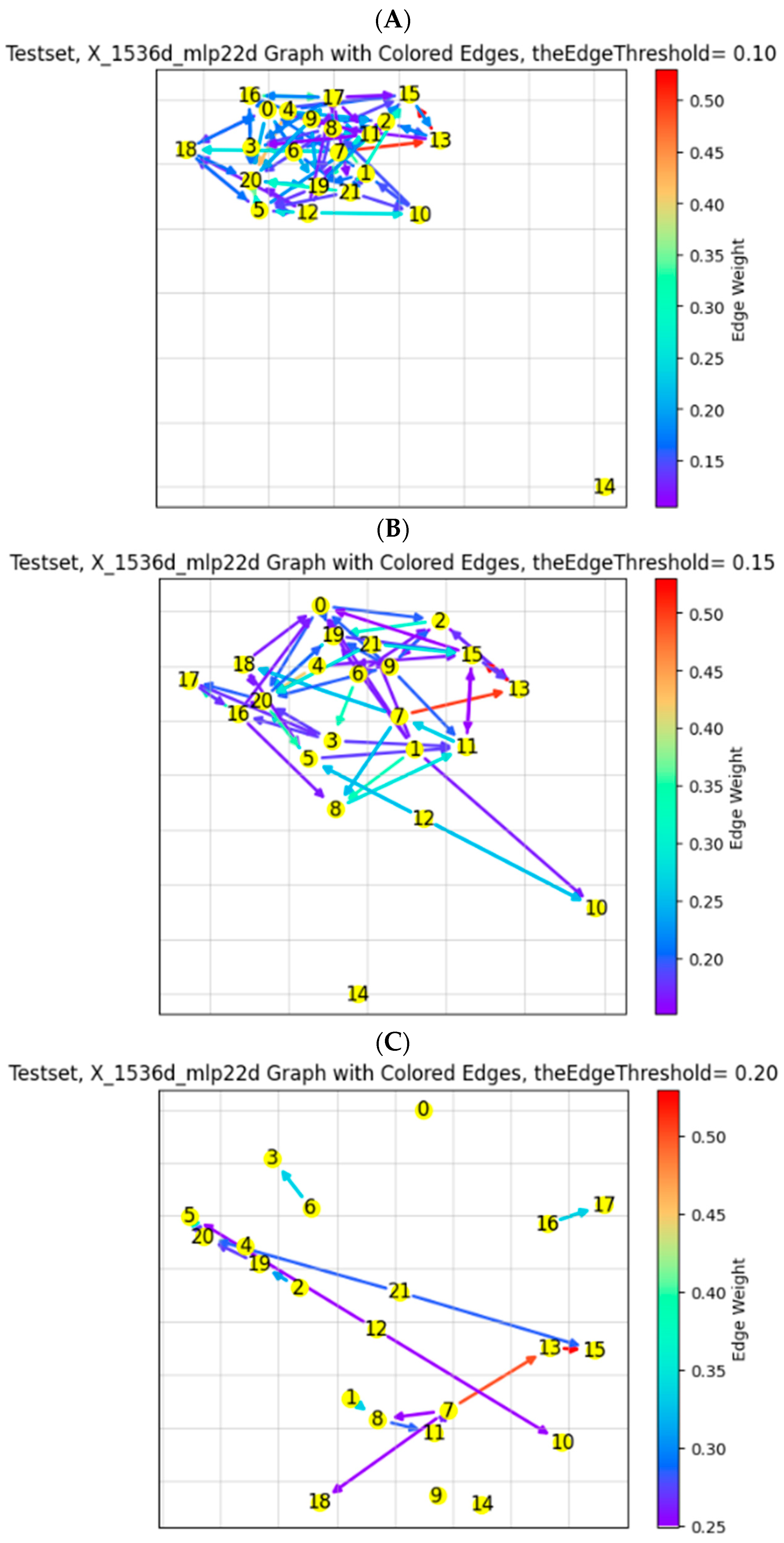
It can be seen in Panel (A) of Figure 10 that the test sample (which is 30% of the total sample) does not present strong connections. Except for very few (light green, orange, or red for conditional probabilities higher than 40%), the majority of the values are very low (dark green, blue, and purple).

Panels (B) and (C) are the same as Panel (A), except that the thresholds are higher (0.15 and 0.20, respectively) and, hence, the number of edges is substantially smaller. We should note that the locations of the vertices are randomly positioned by the software and yet the relationships among them are fixed.

It can be seen from Figure 10 that the 22 financial firms do not form a strong network. The only noticeable connection is that #7 (BlackRock) influences #13 (MetLife), which, in turn, influences #15 (Prudential Financial). Their edge values are over 0.5, where all the other connections are less than 0.5.

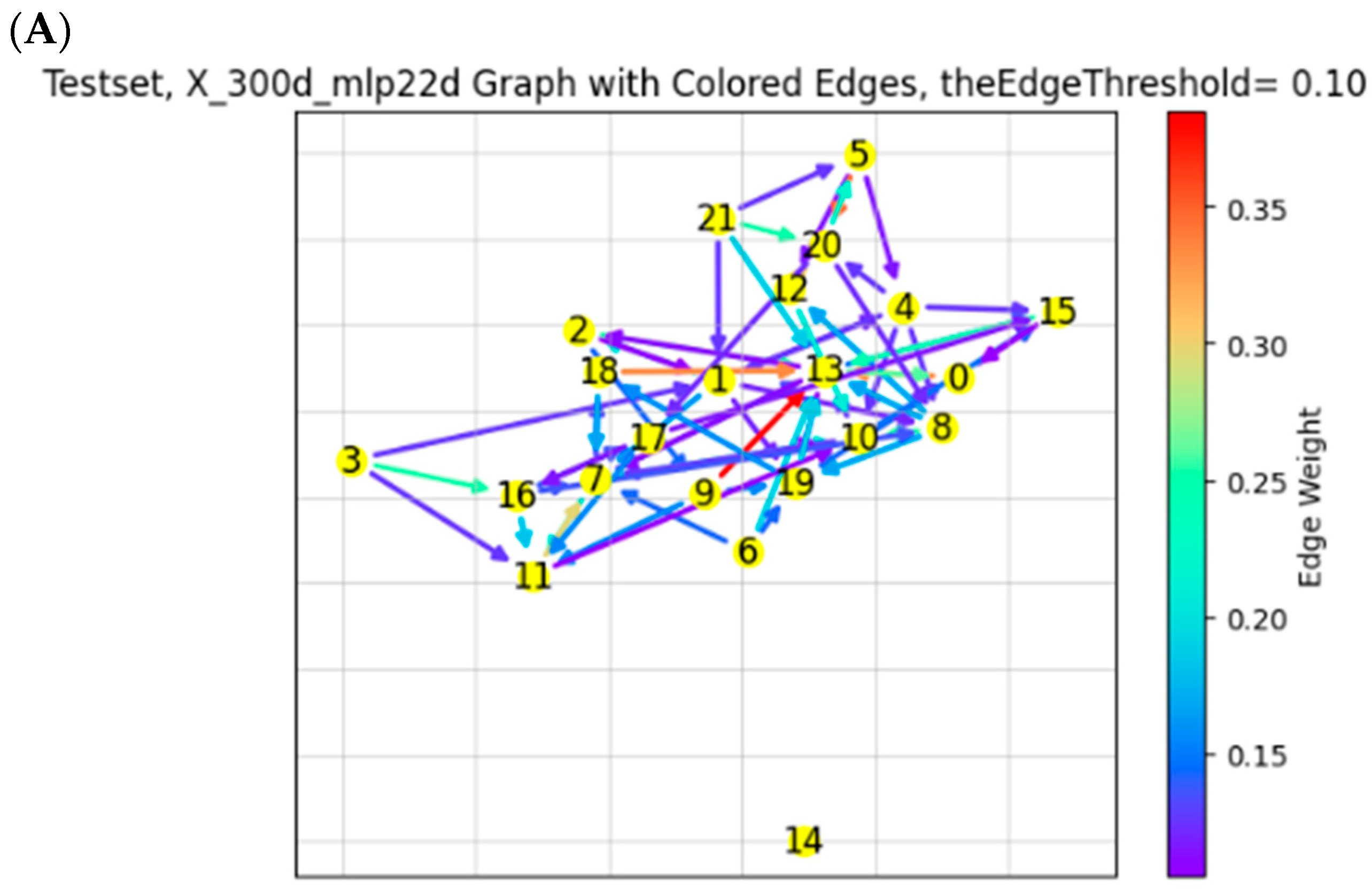
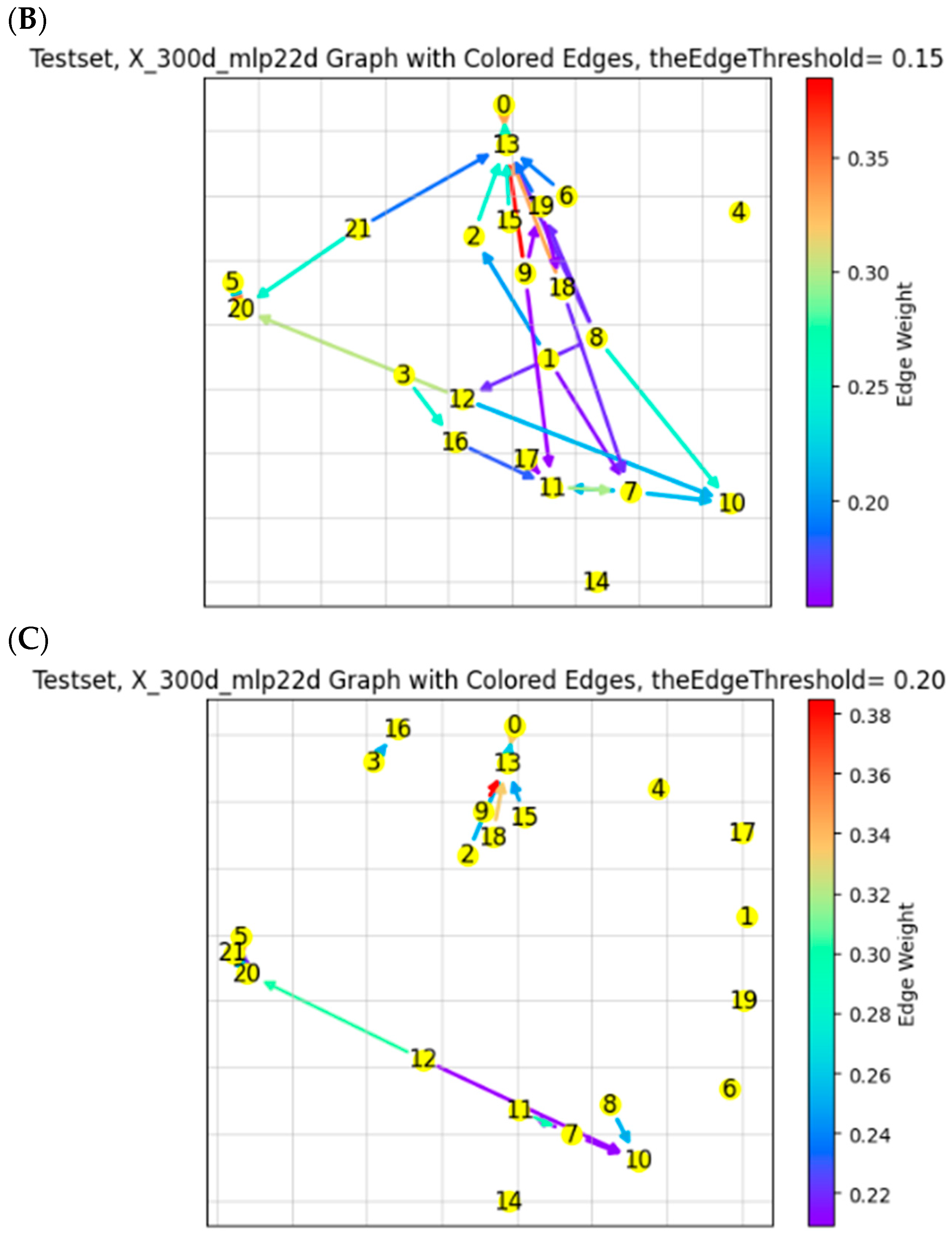
In contrast to the above approach which employs OpenAI and t-SNE, an alternative approach using spaCy and PCA is taken to draw the knowledge graph. Note that spaCy embeds a vector of 300-dimensions (as opposed to 1536 by OpenAI). Then, PCA is used to reduce the vector to two dimensions. The results are given in Figure 11 (confusion matrix) and Figure 12. Again, we should note that row 14 (PNC) is excluded, due to insufficient data, as mentioned earlier, and, hence, the corresponding row in Figure 11 is set to 0.

Figure 12 is qualitatively the same as Figure 10. Except for the connections of firms #9 (Chubb), #13 (MetLife), and #18 (Sate Street), all other firms have very weak relationships. Similar to Figure 10, Panels (A), (B), and (C) are same graphs, except for the different cutoff levels (0.10, 0.15, and 0.20, respectively) for the conditional probability.

Compared to Figure 10 which uses OpenAI and t-SNE, Figure 12 presents a dependency of MetLife (#13) on both Chubb (#9) and State Street (#18). It is logical that Chubb and MetLife are connected, as they are both insurance companies. Interestingly, State Street, although it is an investment firm, holds a substantial holding of Chubb (On 10 February 2023, State Street filed a 13G/A form with the SEC, disclosing ownership of 19.33 MM shares of Chubb Ltd. This represents 4.66% of the company, according to a Nasdaq news release). In fact, State Street invests heavily in the insurance industry. It is clear that different embedding and dimensionality reduction methods lead to different graphs. As a result, it is necessary to perform further certification by the experts in the financial field.

The inconsistency between the two knowledge graphs indicates that the structure of these 22 financial firms is not stable. This is not uncommon in the case of news. To further investigate where the inconsistency lies, we need financial data such as the liquidity discounts used in Chen and Zhang [1]. We will leave this to a future study.

Another possibility for inconsistency is the dataset itself, which contains news for 2016 only. In 2016, there are not substantial global events, unlike 2008 (Lehman crisis) or 2020 (COVID-19 pandemic). In such a “peaceful” period, it is hard to detect any substantial network. It would be ideal to study the 2008 or 2020 news. We will leave this to a future study.

4.6. Comments

Because our results are based on news data from 2016, we do not know the interconnectedness and systemic risk of banks in other years. To roughly address this question, we have downloaded the data of the OFR Financial Distress Index (https://www.financialresearch.gov/financial-stress-index/, accessed on 1 March 2024) and the data from February 2024 from the Kansas City Financial Distress Index (https://www.kansascityfed.org/data-and-trends/kansas-city-financial-stress-index/, accessed on 1 March 2024), to examine whether 2016 was a relatively safe year for the US financial system. The OFR Financial Distress Index provides daily data and covers the period from 2000/1/3 to now. During the whole sample period, the average value and standard deviation of the OFR Financial Distress Index are 0.153 and 4.263, respectively. In the year 2016, the average value and standard deviation of the OFR Financial Distress Index was −0.196 and 1.183, respectively. The Kansas City Financial Distress Index provides monthly data and covers the period from February 1990 to February 2024. The sample mean and standard deviation of the Kansas City Financial Distress Index are 0 and 1, respectively (the index is standardized and, thus, its mean is 0 and its standard deviation is 1). In the year 2016, the average value and standard deviation of the index were −0.163 and 0.284, respectively.

The above numbers indicate that the financial stress index in 2016 was not only much smaller than the historical average, but also had smaller variations. The findings here support our conclusion that there is little systemic risk in the year 2016.

5. Exploring a Large Language Model—ChatGPT4

In this section, we try to use an advanced version of a large language model, such as GPT-4 (or the cheaper version, “gpt-3.5-turbo”), and use LangChain as the platform

5.1. Article Understanding and Summarization

Using the following Python script, we can make a request to OpenAI to perform article understanding and summarization for our long articles. It should be noted that the fees for these services are still high and this is something that researchers must be careful about.

theText = “(a very long article)”

theSummary =

“Fitch Ratings has affirmed the ‘A+’ Insurance Financial Strength (IFS) ratings of Aflac Inc.‘s insurance subsidiaries, as well as Aflac’s Issuer Default Rating (IDR) and senior debt ratings.

The ratings reflect Aflac’s strong competitive position in the supplemental accident and health insurance markets in Japan and the US, as well as its strong earnings profile and capitalization.

However, the outlook for Aflac’s insurance subsidiaries remains negative due to slow economic growth in Japan and the company’s exposure to Japanese sovereign risk. Aflac also faces growing competition in both Japan and the US.”

5.2. Semantic Graph

Using the process described above, we take the first article in the dataset to draw a spring graph containing textual and semantic relationships, as shown in Figure 13.

As can be seen from Figure 13, the node “Aflac” and the node “Fitch Ratings” are the two cores of the entire article. Firstly, we note that “Aflac” is more important than “Fitch Ratings”, because it connects to more other nodes (five for “Aflac” and three for “Fitch Ratings”). Secondly, the connections between nodes (edges) point out the semantic relationships between nodes. For example, the relationship between the node “Aflac” and the node “japan and the US” is an edge for “has important market in”. This is extracted from the text that says “Aflac has important market in Japan and the US”. Similarly, we see that “Aflac has critical leverage ratio of 26% as of 2016”. We should note that Figure 13 is similar to the construction of a graphic database mentioned in the introduction. In other words, LLMs facilitate and empower knowledge graph construction with textual data. This is a potentially interesting area for future research.

These results are quite consistent with the interpretation of human readers (experts). The code is given below:

In the past year (2023), this LLM technology has been regarded, in many fields, as one of the most important AI applications in the future. There is still a lot of room for its use. However, its API call cost is still high at this stage. Therefore, it is difficult for researchers to use it in large quantities, as the following expense list shows.

6. Conclusions, Limitations, and Future Research

In this paper, we draw knowledge graphs of news from 2016 of the top 22 financial firms. Such graphs are useful in examining the vulnerability in the financial system, also known as systemic risk. News articles, different from distress index or volatility used in the literature (see Chen and Zhang [1]), are used in drawing the graphs. As a result, we adopt different embedding methods that are pertained to textual analysis. We also explore various embedding methods.

One novel contribution of this paper is that we use OpenAI tools, which are the same tools used by ChatGPT, the most recent product by OpenAI. Using OpenAI’a api, we can access the tools used by ChatGPT. The drawback is that this is a paid service and can become quite expensive if the usage is heavy.

Using textual data for analyzing financial systemic risk is new, yet it is intuitive that news should be a timely reflection of how financial institutions are connected. Anecdotal evidence from the 2008 Lehman crisis indicates that media were heavily used by the short side to spread rumors and then take advantage of the plummets of the stock market.

The major drawback of our paper is its data. We are limited to only 2016 news articles of about 1600 companies, provided by LexisNexis. There are three limitations with this data, as follows: (1) the data are too few to conduct any migration analysis, commonly used in banking risk management; (2) we cannot make any comparison of our results with those in the literature, which does not cover 2016; and (3) 2016 is a rather uneventful year and, consequently, the knowledge graphs do not properly reflect the vulnerability of the networks. Further research should focus on the periods where financial institutions are highly connected.