Detection and Classification of Cannabis Seeds Using RetinaNet and Faster R-CNN

Abstract

The rapid growth of the cannabis industry necessitates accurate and efficient methods for detecting and classifying cannabis seed varieties, which is crucial for quality control, regulatory compliance, and genetic research. This study presents a deep learning approach to automate the detection and classification of 17 different cannabis seed varieties, addressing the limitations of manual inspection processes. Leveraging a unique dataset of 3319 high-resolution seed images, we employ self-supervised bounding box annotation using the Grounding DINO model. Our research evaluates two prominent object detection models, Faster R-CNN and RetinaNet, with different backbone architectures (ResNet50, ResNet101, and ResNeXt101). Extensive experiments reveal that RetinaNet with a ResNet101 backbone achieves the highest strict mean average precision (mAP) of 0.9458 at IoU 0.5–0.95. At the same time, Faster R-CNN with ResNet50 excels at the relaxed 0.5 IoU threshold (0.9428 mAP) and maintains superior recall. Notably, the ResNeXt101 backbone, despite its complexity, shows slightly lower performance across most metrics than ResNet architectures. In terms of inference speed, the Faster R-CNN with a ResNeXt101 backbone demonstrates the fastest processing at 17.5 frames per second. This comprehensive evaluation, including performance-speed trade-offs and per-class detection analysis, highlights the potential of deep learning for automating cannabis seed analysis. Our findings address challenges in seed purity, consistency, and regulatory adherence within the cannabis agricultural domain, paving the way for improved productivity and quality control in the industry.

1. Introduction

Cannabis, a widely cultivated and consumed plant, has garnered significant attention in recent years due to its medicinal and recreational properties. With the increasing legalization and commercialization of cannabis products, there is a growing need for efficient and accurate methods to detect and classify cannabis seeds [1]. Traditional manual sorting and classification processes are labor-intensive, time-consuming, and prone to human error. In response to these challenges, deep learning, a subset of artificial intelligence, has emerged as a promising solution. Integrating advanced technologies, such as deep learning and computer vision, in this sector is paramount. In the context of seed detection and classification, particularly for cannabis seeds, these technologies offer significant benefits. Automating manual processes can enhance productivity and quality control, ultimately improving efficiency in tasks such as seed sorting and quality testing. The detection of cannabis seeds can significantly reduce the labor and time required for seed identification, benefiting farmers and researchers alike. It allows for the precise classification of seeds, helping farmers identify the specific variety of cannabis they are dealing with. Cannabis seed detection holds particular significance compared to other seed detection processes due to the unique characteristics and legal considerations surrounding cannabis cultivation. Unlike many other crops, cannabis varieties vary significantly in their chemical composition, particularly in the concentration of psychoactive compounds such as THC. As a result, the accurate identification of cannabis seeds is crucial for regulatory compliance and ensuring that seeds are cultivated within legal limits.

The growing popularity of cannabis for both medicinal and recreational purposes has led to increased demand for accurate seed detection methods to maintain product quality and consistency. Many studies have tried to define Cannabis sativa L. based on its appearance and chemical properties. The accepted taxonomy identifies two subspecies—sativa and indica. Each subspecies has two main varieties—cultivated and wild. The most important varieties for medicine are C. sativa ssp. sativa var. sativa (known as C. sativa) and C. sativa ssp. indica var. indica (known as C. indica). There is also a third, less common variety called C. sativa ssp. sativa var. spontanea, known as C. ruderalis. C. indica is usually grown for recreational purposes, while C. sativa is increasingly recognized for its potential medical applications [2]. These distinctions are crucial in understanding the diverse applications of cannabis. Industrial hemp and marijuana are distinct subtypes of the Cannabis sativa species, primarily differentiated by their use, chemistry, and cultivation methods. Industrial hemp is mainly based on the quantity of THC, the psychoactive component present in the plant. While 1% THC is usually enough to produce intoxication, several regions legally differentiate between marijuana and hemp based on the 0.3% THC threshold [3]. Hemp is grown for industrial purposes, such as fibers, textiles, and seeds, and contains a very low level of the psychoactive compound ${∆}^9$-tetrahydrocannabinol (THC) [4]. In contrast, marijuana is cultivated for its THC-rich flowers and extracts, primarily for recreational or medicinal use, and it is selectively bred for high THC concentrations. The key difference lies in their intoxicating potential, with hemp having negligible THC content [5].

Artificial intelligence methods have been increasingly applied to various aspects of cannabis agriculture in recent years. Seed classification has been a topic of extensive research, with studies employing various approaches including traditional manual methods [6,7,8,9], image processing techniques [10,11,12,13,14,15], and modeling techniques [16,17,18,19,20,21,22,23]. On the other hand, Sieracka et al. [24] utilized artificial neural networks to predict industrial hemp seed yield based on cultivation data, showcasing the potential of AI in optimizing hemp production. In a different application, Bicakli et al. [25] demonstrated the effectiveness of random forest models in distinguishing illegal cannabis crops from other vegetation using satellite imagery, which could aid in monitoring and regulation efforts. Ferentinos et al. [26] introduced a deep learning system that leverages transfer learning to identify diseases, pests, and deficiencies in cannabis plant images, highlighting the potential of AI in early detection and intervention. More recently, Boonsri et al. [23] applied deep learning-based object detection models to differentiate between male and female cannabis seeds from augmented seed image datasets, demonstrating the ability of AI to assist in gender-based seed sorting. Despite these advancements, applying deep learning techniques for cannabis seed variety detection and classification remains an area with untapped potential, warranting further research and exploration. However, traditional manual methods are often time-consuming and labor-intensive, relying on visual inspection and biochemical analysis. Image processing techniques have improved accuracy but struggle with handling variations in seed appearance and imaging conditions. Machine learning and deep learning approaches, categorized as modeling techniques, have achieved high accuracy but often lack robustness and primary data, particularly when classifying extremely similar seeds. Furthermore, many studies rely on a limited set of features for classification and fail to address the need for standardized evaluation metrics and benchmarks. Another key challenge that researchers faced was the variability in seed quality and genetics, which can impact the reproducibility and reliability of research findings. Ensuring seed purity and genetic stability is crucial but can be difficult due to the lack of standardized seed certification and analysis methods. However, to overcome these challenges, this research builds upon and significantly extends our previous work on cannabis seed variant detection using Faster R-CNN. While our previous study [27] focused solely on the Faster R-CNN architecture with a ResNet50 backbone and explored various loss functions, the current research broadens the scope considerably. We now aim to include a comprehensive comparison between Faster R-CNN and RetinaNet, incorporate additional backbone architectures (ResNet101 and ResNeXt101), and integrate the insights gained from our previous loss function analysis. This expanded investigation aims to provide a more thorough understanding of deep learning approaches for cannabis seed detection and classification. 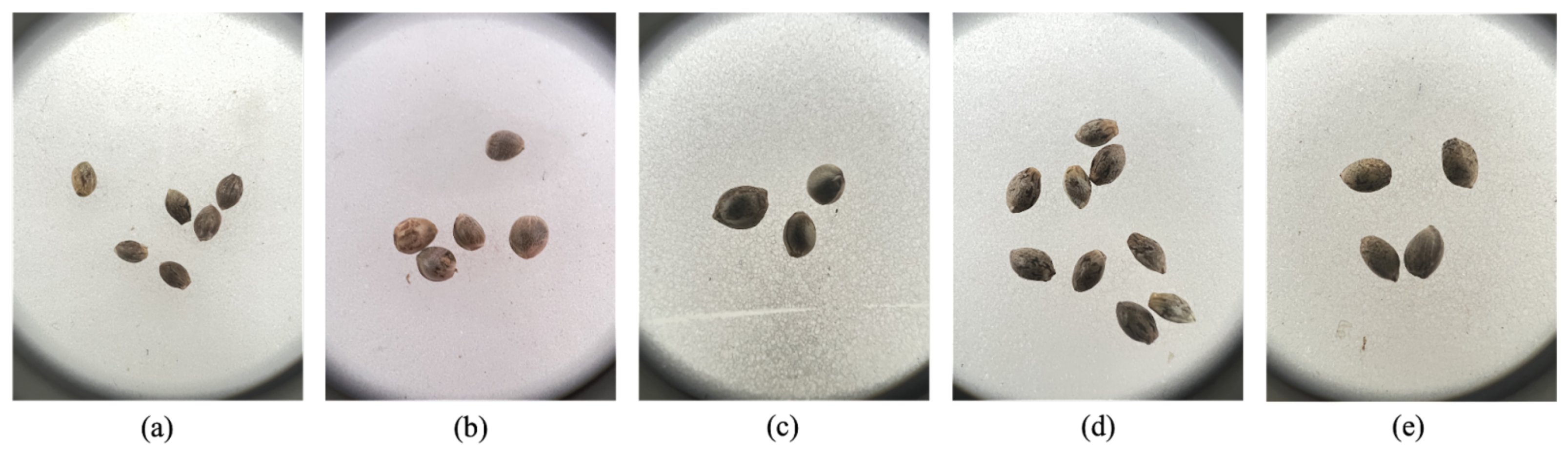The dataset [28] used in this study is a collection of cannabis seed variants from 17 different categories, which was used in our previous study [27] as well. The main objective of this paper is to classify seeds of these 17 kinds of cannabis. Our study aims to fill previous research gaps by utilizing deep learning algorithms to precisely identify and outline the bounding box regions of various cannabis seed varieties. Key contributions of this research are given below:

• Extension of our previous work on cannabis seed detection, incorporating additional object detection architectures (RetinaNet alongside Faster R-CNN) and expanding the analysis scope.
• Unlike previous studies, which focused on limited seed varieties [23], this research classifies seeds from 17 different cannabis varieties, providing in-depth metrics on detection accuracy and processing speed.
• Integration of optimal loss functions identified in our earlier study, applied to an expanded set of model configurations.
• This study employs state-of-the-art deep learning models, including ResNet 50, ResNet 101, ResNext 101, and RetinaNet, to enhance the accuracy and efficiency of cannabis seed detection and classification.
• Validation and extension of our previous findings, offering refined insights into effective deep learning approaches for cannabis seed classification and detection.

The paper is structured as follows: Section 2 delves into the related work, providing an overview of prior research in the field. Section 3 outlines the dataset used, along with the data pre-processing steps and the training methodology employed. Section 4 elaborates on the object detection models, including their architectures and the backbone networks utilized in our experiments. The experimental results are presented in Section 5, where we discuss our findings and compare the performance of the various object detectors. In Section 6, we presented the discussion, and, finally, Section 7 presents the conclusions of this research.

2. Related Work

Several studies have already been done on seed classification. We can divide them into three categories: the traditional (manual) method, image processing, and modeling. The traditional method [6,7,8,9] of seed classification involves visual inspection, biochemical seed identification, machine vision, and DNA analysis for accurate categorization. Additionally, image processing methods are, again, divided into three categories: structural method [10,11,12], threshold method [13,29,30], and spectral method [14,15,31]. The structural method analyzes patterns, shapes, and relationships between different image elements to extract meaningful information and enhance understanding. In contrast, the threshold method concerns setting a specific intensity level, or threshold, to segment an image into different regions based on pixel values. On the other hand, the spectral method involves the analysis of different wavelength bands within the electromagnetic spectrum. The modeling technique usually learns patterns and features from a labeled dataset. Machine learning and deep learning are the most common modeling techniques for classification. These models, often convolutional neural networks, extract hierarchical representations of an image. During training, the model adjusts its parameters to minimize the difference between predicted and actual labels. Once trained, the model can generalize its learned patterns to detect objects or features in new, unseen images. In seed detection and classification, several works have been conducted on machine learning [16,17,18,19,32,33], and deep learning [20,21,22,34,35,36,37]. In Figure 1, we summarize works conducted on seed detection and classification.

While previous research on cannabis agriculture has employed deep learning methods that have demonstrated potential in the gender screening of cannabis seeds [23], their effectiveness in discriminating between seed varieties has not been investigated. Additionally, this study has not categorized their research into multiple classes of seeds. In image processing, Ahmed et al. [10] worked on applying X-ray CT scanning to pepper seed analysis, employing recycling, feature extraction, and classification to robustly categorize seeds into viable and nonviable groups. Pereira et al. [11] addressed soybean seed quality challenges, introducing an image analysis framework that significantly enhanced vigor classification, achieving 81% accuracy. Meanwhile, Zhang et al. [12] innovatively utilized deep learning and edge detection for internal crack detection in corn seeds, presenting the optimized S2ANet model with 95.6% average precision. However,

Table 1. Advancements and limitations of seed classification and detection in modeling.

Ref.	Contributions	Algorithms	Accuracy	Limitation
Luo et al. [34]	Created a nondestructive intelligent picture identification system using deep convolutional neural network models like AlexNet and GoogLeNet to reliably detect 140 weed seed species.	AlexNet, GoogLeNet, VGG-16, SqueezeNet, Xception	93.11%	Detection robustness of the proposed method
Khan et al. [16]	Implemented machine learning algorithms to classify dry beans.	LR, NB, KNN, DT, RF, XGB, SVM, MLP	95.4%	Bean suture axis was ignored due to its enormous time requirement.
Dubey et al. [36]	Applied machine learning model to classify the variety of the wheat seed.	ANN	88%	Their accuracy could be better.
Cheng et al. [21]	Machine learning applications have been applied to detect the defect of the rice seed.	Back-propagation neural network	91–99%	The algorithm could be better.
Heo et al. [37]	Developed a super-high purity seed sorting system with 500-fps throughput, using low-latency deep neural network image recognition	Yolo	99.81%	This method can be applied to acquire clean seed samples.
Bi et al. [38]	Developed an automatic maize seed identification model using transformer and deep learning.	AlexNet, Vgg16, ResNet50, Visio-Transformer, Swin-Transformer	96.53%	The model’s capability of classifying seeds that are extremely similar still requires further improvement.
Madhavan et al. [20]	Created a model for post-harvest classification of wheat seeds.	ANN	96.7%	No primary data.
Javanmardi et al. [22]	Applied machine learning for corn seed classification.	CNN, ANN	98.1%	No primary data.
Ali et al. [17]	Applied machine learning for corn seed classification.	MLP, LB, RF, BN	98.93%	Few features for classification.
Jamuna et al. [19]	Classification of cotton seed quality based on different growth stages.	NB, MLP, J48	98.78%	No primary data.

shows a compact summary of the contributions of seed classification and detection by modeling techniques.

Table 1 provides an overview of various research contributions in the field of seed classification using machine learning and deep learning algorithms. Luo et al. [34] introduced a nondestructive intelligent image recognition system employing deep CNN models like AlexNet and GoogLeNet, achieving a notable accuracy of 93.11% in detecting 140 weed seed species. Their study proposes a solution through nondestructive intelligent image recognition. An image acquisition system captures and segments images of single weed seeds, forming a dataset of 47,696 samples from 140 species. Their research emphasizes the importance of selecting a CNN model based on specific identification accuracy and time constraints. A notable limitation of this study is the robustness of the proposed detection method. Khan et al. [16] worked on classifying dry beans using machine learning algorithms such as LR, NB, KNN, DT, RF, XGB, SVM, and MLP, achieving a high accuracy of 95.4%, with the limitation being the considerable time requirement for ignoring the bean suture axis. Dubey et al. [36] applied an artificial neural network to classify wheat seed varieties with an accuracy of 88%, highlighting the space for improvement in accuracy. Cheng et al. [21] used machine learning for rice seed defect detection, employing Principal Component Analysis and a back-propagation neural network with an accuracy range of 91–99%, suggesting potential improvements in the algorithm. Lawal [39] proposed a deep learning model for fruit seed detection using YOLO, achieving 91.6% accuracy, with the need for accuracy enhancement specifically in the YOLO Muskmelon model. Heo et al. [37] developed a high-throughput seed sorting system using YOLO, reaching an impressive accuracy of 99.81%, showcasing its potential for acquiring clean seed samples. Bi et al. [38] focused on maize seed identification, employing a range of algorithms such as AlexNet, Vgg16, ResNet50, Visio-Transformer, and Swin-Transformer, achieving the best accuracy of 96.53%. However, their work identified a need for improvement in classifying extremely similar seeds. Madhavan et al. [20] conducted post-harvest classification of wheat seeds using artificial neural networks and achieved an accuracy of 96.7%, but their study lacked primary data. Javanmardi et al. [22] concentrated on corn seed classification, employing CNN and ANN, achieving a good accuracy of 98.1%. Ali et al. [17] explored corn seed classification using various machine learning algorithms, including MLP, LB, RF, and BN, achieving a high accuracy of 98.93%, but faced limitations due to the scarcity of features for classification. Jamuna et al. [19] focused on cotton seed quality classification at different growth stages, utilizing algorithms like NB, MLP, and J48, achieving an accuracy of 98.78%, with the limitation of lacking primary data in their study.

While seed analysis has been explored using various techniques, research specifically focused on cannabis seed detection and classification remains limited. Boonsri et al. [23] made initial strides in this field by classifying a limited number of cannabis seed varieties using convolutional neural networks. However, their work, along with other studies in seed object detection, revealed several persistent gaps. These include limited publicly available datasets, inadequate methods for handling variations in seed appearance and imaging conditions, and a lack of standardized evaluation metrics and benchmarks. Additionally, existing approaches often rely on traditional computer vision methods that may struggle with complex seed shapes and textures. To address these research gaps, we initiated a comprehensive study on cannabis seed detection and classification. Our previous work [27] laid the groundwork in this domain by exploring the use of Faster R-CNN for detecting and classifying 17 varieties of cannabis seeds. Using a locally sourced dataset from Thailand, we investigated various loss functions (L1, IoU, GIoU, DIoU, and CIoU) with a ResNet50 backbone, achieving a mAP score of 94.08% and an F1 score of 95.66%. This study emphasized the importance of accurate seed variant identification for precision breeding, regulatory compliance, and meeting diverse market demands. Building upon our previous research, the current study aims to further advance the field of cannabis seed detection and classification. We expand our investigation to include multiple object detection architectures and backbone networks, providing a more comprehensive analysis of state-of-the-art deep learning techniques in this domain.

3. Methods and Materials

Building upon our previous work [27], we have significantly expanded our methodology to provide a more comprehensive analysis of cannabis seed detection and classification techniques. Our current study extends the investigation in two key areas. First, while our previous study focused exclusively on the two-stage Faster R-CNN model, we now include RetinaNet, a one-stage detector alternative. This addition allows us to compare the performance of different architectural approaches in the context of cannabis seed detection. Second, we have broadened our evaluation of backbone networks. In addition to the ResNet50 used in our previous work, we now assess the performance of ResNet101 and ResNeXt101. This expansion aims to identify potential improvements in feature extraction and overall model performance. To ensure consistency and enable direct comparisons with our previous findings, we utilized the same dataset of 17 cannabis seed varieties as in our earlier study.

3.1. Data Description

The dataset [28] utilized in this study is a collection of cannabis seed varieties encompassing 17 distinct categories. These seeds are readily available in Thailand. To the best of our knowledge, this dataset is the first of its kind to be made publicly accessible, and this research utilized this dataset for cannabis seed classification. Captured using an Apple iPhone 13 Pro, the dataset comprises 3335 high-resolution photos with dimensions of 3023 × 4032 pixels, reduced to 3319 after excluding blurred images. All photos feature a white backdrop but were taken from various angles and under different lighting conditions.

Table 2. Original dataset provided by [28].

Seed Variant	Abbreviation	Number of Collected Images
AK47 photo	AK47	106
Blackberry (Auto)	BBA	203
Cherry Pie	CP	50
Gelato	GELP	327
Gorilla Purple	GP	554
Hang Kra Rog Ku	HKRKU	153
Hang Kra Rog Phu Phan ST1	HKRPPST1	249
Hang Suea Sakon Nakhon TT1	HSSNTT1	93
Kd	KD	49
Kd_kt	KDKT	147
Krerng Ka Via	KKV	141
Purple Duck	PD	151
Skunk (Auto)	SKA	233
Sour Diesel (Auto)	SDA	327
Tanaosri Kan Daeng RD1	TKDRD1	157
Tanaosri Kan Kaw WA1	TKKWA1	183
Thaistick Foi Thong	TFT	212
Total		3335

presents the seed types along with the number of images collected, and Figure 2 provides examples of several cannabis seed varieties.

3.2. Data Pre-Processing

3.2.1. Bounding Box Annotation

Instead of manually labeling each image, which is both time-consuming and labor-intensive, we opted for a more efficient approach using Grounding DINO [40] in this research, which is an open-set object detector. Grounding DINO takes an input image and associated noun phrases to generate multiple two-dimensional bounding boxes corresponding to the objects identified within the image. The model uses a robust mechanism for grounding, which involves associating visual features with the provided noun phrases, enabling it to localize and accurately label objects, even in unfamiliar contexts. This process involves several stages, including feature extraction, where the image is analyzed to extract high-level features, and transformer-based decoding, where these features are matched with the noun phrases to produce bounding boxes. The bounding boxes generated are then refined to ensure precision, allowing for automatic and efficient annotation of large datasets without the need for manual labeling. Unlike traditional object detectors, open-set detectors like Grounding DINO can identify object categories beyond those on which they were specifically trained. This capability enables the model to generate multiple 2D bounding boxes for an input image based on associated noun phrases. By utilizing Grounding DINO, we could automatically extract object boundaries from the dataset without the need for manual annotation, as the model could identify and delineate object instances based on the provided text queries. In this research, we added “all seeds” as text queries. Figure 3 illustrates an example of bounding boxes applied to our cannabis seed dataset.

3.2.2. Data Augmentation

Data augmentation is a crucial technique employed to enhance dataset size, particularly in scenarios where data availability is limited [41]. By applying various image transformations, the model’s ability to generalize to unseen data is improved, especially during the validation phase. These transformations include geometrical transformations, color adjustments, and blur operations. Geometrical transformations encompass random horizontal or vertical flips, translations in both horizontal and vertical directions, resizing to different scales, and rotations. Color adjustments involve modifying brightness and contrast, altering the values of red, green, and blue channels, randomizing hue, saturation, and value, and shuffling the order of RGB channels. Blur operations entail applying random blur or median blur to the image. Implementation of these augmentation techniques is facilitated using the Albumentations library [42]. Specifically, the augmentation settings included random flips with a 50% probability, a maximum image shift of 0.0625, a maximum scale change of 0.1, and a maximum rotation angle of 45 degrees. Furthermore, brightness and contrast were randomly adjusted between 0.1 and 0.3 with a 20% chance, shifts in RGB channels up to 10 intensity levels each, and maximum changes in hue, saturation, and value of 20, 30, and 20, respectively, for 10% of the images. Additional augmentation parameters included a 10% probability of channel shuffling and a 10% probability of applying random blur or median blur with a maximum kernel size of 3 during image augmentation. Before data augmentation, we implemented an efficient annotation process using Grounding DINO [40], an open-set object detector. This approach significantly reduced the manual labor typically associated with bounding box annotation. Grounding DINO leverages natural language prompts to identify and localize objects in images, even for categories it was not explicitly trained on. For our cannabis seed dataset, we used prompts such as ’cannabis seed’ or a specific variety of names to generate bounding boxes automatically. This method proved particularly effective for our large dataset of 3319 high-resolution seed images, ensuring consistent and accurate annotations across all 17 cannabis seed varieties. The Grounding DINO model’s ability to generalize to unseen object classes made it ideal for our diverse seed dataset, providing a solid foundation for subsequent object detection tasks.

3.2.3. Splitting of the Dataset

Following the annotation process, we divided the dataset into three subsets: training, validation, and test sets in this research.

Table 3. Quantity of images and instances per seed type in the training, validation, and testing datasets.

Seed Variety	Training Images	Training Instances	Validation Images	Validation Instances	Test Images	Test Instances
AK47	57	321	21	123	28	160
BBA	113	565	34	170	55	275
CP	22	67	11	33	17	57
GELP	178	894	70	350	79	400
GP	303	909	125	375	126	378
HKRKU	83	427	38	190	32	160
HKRPPST1	123	693	61	337	64	355
HSSNTT1	39	265	18	122	34	234
KD	39	195	6	30	3	15
KDKT	82	562	42	278	23	171
KKV	65	325	37	185	34	170
PD	76	380	36	180	37	185
SKA	117	585	49	245	67	335
SDA	167	668	69	276	89	356
TKDRD1	93	465	29	145	34	170
TKKWA1	101	553	32	174	49	267
TFT	113	589	45	233	54	270
Total	1771	8463	723	3446	825	3958

provides a breakdown of the number of images per seed variety and the distribution across the three subsets. Approximately 53% of the dataset, consisting of 1771 images, was allocated for training our object detection models. During the training process, we used around 22% of the dataset, comprising 723 images, for validation purposes to assess the model’s performance. The remaining 25% of the dataset, 825 images in total, was set aside for testing the trained model’s performance on unseen data. This approach ensures a robust evaluation of the model’s generalization capabilities.

3.3. Training of the Dataset

In this study, we employed PyTorch in conjunction with the mmdetection object detection toolbox [43] to train two distinct models, namely Faster R-CNN and RetinaNet, utilizing the computational power of an NVIDIA RTX 3090 GPU. The initialization of these models involved leveraging weights pre-trained on the COCO dataset [44], a common practice to benefit from the knowledge gained from a large-scale dataset. To ensure uniformity in input dimensions, all images were resized to 360 pixels in width and 640 pixels in height. The training regimen spanned 100 epochs and employed stochastic gradient descent (SGD) optimization. A learning rate of 0.02 was assigned to Faster R-CNN, while RetinaNet was optimized with a slightly lower learning rate of 0.01. To prevent overfitting and ensure model stability, weight decay was set to 0.0001, and momentum was fixed at 0.9. The choice of batch sizes was crucial for efficient training: a batch size of 2 was used for training, 1 for validation, and 1 for testing. In this study, we implemented multi-stage learning rate strategies, specifically employing Linear Decay and Cosine Annealing schedules, to dynamically adjust the learning rate during the training of our Faster R-CNN and RetinaNet models. The Linear Decay scheduler reduces the learning rate at the outset of training by multiplying the original learning rate with a predefined factor. Subsequently, it gradually increases the learning rate back to its original value over a specified number of training steps. For our experiment, we set the multiplying factor to 0.001 and the number of training steps to 500. Conversely, using a cosine function, the Cosine Annealing scheduler facilitates a smooth decay of the learning rate. This scheduler commences by decreasing the learning rate until it reaches a minimum value. In our experiment, we set this minimum learning rate to 0 and determined that the learning rate decayed over a maximum of 100 epochs. After each training epoch, model performance was evaluated using the validation dataset. Predictions were considered positive if they achieved an Intersection over Union (IoU) threshold of 0.5, below which they were classified as negative. To preserve the best-performing model, checkpoints were saved based on the evaluation metric, ensuring that the final model selected for evaluation was the most optimal.

Figure 4 illustrates the proposed workflow for this research. Initially, the dataset is divided into three subsets: training, testing, and validation. The training set is utilized to train the object detection model, while the testing set is used to evaluate its performance. Subsequently, the training data undergo data augmentation to enhance the model’s ability to generalize to unseen data. Following data augmentation, the object detection model is applied to the augmented data to perform detection tasks. The results of the detection process are then analyzed to evaluate the model’s performance.

4. Object Detection Models

4.1. RetinaNet Network Architecture

RetinaNet [45] is a one-stage object detector with a backbone network and two task-specific subnetworks (see Figure 5). The backbone network extracts the hierarchical feature representations from the input images. The first subnetwork is responsible for the object classification, and the second subnetwork is a regressor that generates the bounding box coordinates. Next, we describe the individual components of RetinaNet. We used three backbones, ResNet50, ResNet101, and ResNeXt101 [46], in our RetinaNet architecture. All of these backbones were pre-trained on ImageNet. The backbone’s features from each convolution block were then used as input for the next component, the feature pyramid network (FPN).

RetinaNet uses a feature pyramid network [45] to construct a multi-scale feature pyramid using the output from different convolution blocks of the backbone network (Figure 5). It starts by creating an upsampling path from the lower-resolution features in the top layers of the backbone to the higher-resolution layers at the bottom. This top–down pathway is merged with the bottom–up feature maps from the backbone layers using lateral connections. We used three 1 × 1 lateral convolutions that reduce the bottom–up feature maps (512, 1024, and 2048) from the backbone to a 256-channel output and connected them with the upsampled top–down feature maps. The merged features then passed through five 3 × 3 convolutions that we applied to output five 256-channel feature maps in the feature pyramid. At each pyramid level, we used a predefined set of anchor boxes as reference boxes as criteria to classify object/non-object and as bounding box regression targets. The anchors had aspect ratios of (1:2, 1:1, and 2:1) in each pyramid level. Each anchor had a length of 17 one-hot vectors to classify the object class and a vector with length four as a regression target. We attached two separate fully connected networks—classification and regression subnetworks—to each level of the feature pyramid and applied four 3 × 3 convolutional layers, each with 256 channels, followed by another 3 × 3 convolution to the feature maps with 256 channels. The classification subnetwork predicted the probability of a class object present at each anchor box. We then applied sigmoid activations in the classification layer to get binary predictions per anchor box. Meanwhile, the box regression subnetworks refined the anchor box coordinates to localize the objects and output four vectors per anchor box. To optimize RetinaNet, we used Focal loss for the classifications and L1 loss for the regressions.

4.2. Faster R-CNN Network Architecture

There are five parts to Faster R-CNN [48], which is an object detector with two stages. Step one of the Faster R-CNN process involves the network components known as the backbone, feature pyramid, and region proposal. Step two of the Faster R-CNN pipeline is the region of interest align, classifier, and bounding box regressor.

The Faster R-CNN network (Figure 6) is built using a ResNet50 [49] model that has already been trained on ImageNet. By presenting the idea of skip connections, residual networks address the vanishing gradients issues that plague extremely large convolutional networks. The idea behind skip connection is to shorten the gradient flow during training by skipping activations of earlier levels and going straight to one or more layers after it. The feature pyramid network’s bottom–up approach begins with the backbone, the first processing layer. It extracts features from the input picture at many intermediary stages. To determine the level of the pyramid, a feature pyramid network [50] uses features produced by the final residual blocks of the ResNet 50 backbone’s conv2, conv3, conv4, and conv4 operations. It aids the model in spotting things in pictures of varying sizes. FPN establishes a lateral link between the bottom–up and top–down pathways. From the bottom–up pyramid stages, our FPN reduced the four output feature maps (256, 512, 1024, and 2048) to fixed 256-channel outputs using four lateral 1 × 1 convolutions combined with the upsampled top–down route. Using the combined feature map as input, we ran four 3 × 3 convolutions, which produced a four-tiered feature pyramid with 256-channel feature maps at each tier.

The region proposal network (RPN) receives feature maps from the FPN [51]. The feature pyramid extracts maps of features that the RPN uses to run a small network. The 256-channel feature map that came from the convolutional layer was fed into our RPN head using a 3 × 3 convolution with 256 channels, which was then activated using ReLU. At each point along the sliding window that covers the feature map, RPN employed anchor boxes to produce a group of potential regions with varying sizes and aspect ratios. Using one scale (8) and three aspect ratios (1:2, 1:1, and 2:1), our anchor generator generated regional solutions for each sliding window. The RPN layer used these candidate proposals’ objectness scores to filter them; therefore, they were not final. How much of an object or background is in the region’s proposal was determined by its objectness score. Two completely linked layers, box classification and box-regression, were fed each area suggestion. A 1 × 1 256-channel convolution layer was used for classification after the convolution layer, and a parallel 1 × 1 12-channel convolution layer was used to regress the coordinates of the bounding boxes. The objectness value for each area suggestion was generated by the first layer, a binary classifier that used the Intersection over Union metric. In the second layer, the region proposal’s bounding box was constructed. The bounding box regression layer employed L1 loss for classification, whereas the sigmoid outputs were used to compute cross-entropy loss for classification. To cut down on redundant region recommendations, we used non-maximum suppression according to their classification scores. We removed boxes with significant levels of overlap and kept no more than 1000 region suggestions per picture, setting the IoU threshold for NMS at 0.7. Varieties of size and aspect ratio were produced by the RPN’s region suggestions. The Fast R-CNN branch took in proposals and used four ROI align [52] layers to extract features. Each feature was a fixed size of 7 × 7 and was produced by the branch. Using ROI pooling in the original Faster R-CNN study, a fixed-length feature vector was generated from each area suggestion. However, since ROI align could fix the round-off mistakes that ROI pooling made, we opted to employ it instead. ROI align took the region suggestions and utilized max-pooling and bilinear interpolation to get fixed-length feature vectors. One fully connected layer used the 7 × 7 feature vector from the ROI align to forecast the class score using cross-entropy loss. In contrast, the other used regression to forecast the position of the bounding box. We considered the suggestion a success if the IoU was higher than the cutoff value of 0.5. L1 loss, IoU loss, Generalized IoU loss, Distance IoU loss, and Complete IoU loss were among the five loss functions employed to minimize the regression layer’s loss in the bounding box regressor layer.

5. Experimental Evaluation

5.1. Evaluation Metrics

In our experiments, we used four evaluation metrics [53] to evaluate the performance in our object detection models. These metrics included Intersection over Union, mean average precision, recall, and F1. These metrics are defined as follows.

5.1.1. Intersection over Union (IoU)

Intersection over Union is the most commonly used metric to assess the bounding box prediction object detection task quality. IoU quantifies the similarity of the predicted bounding box to the ground truth bounding box. The IoU is the ratio between the area of overlap between the ground truth bounding box and the predicted bounding box and the union area of these two bounding boxes. Equation (1) provides the formula to derive the IoU. In this context, GT is the ground truth bounding box, and PB is the predicted bounding box.

$$IoU={\displaystyle \frac{Area(GT\cap PB)}{Area(GT\cup PB)}}$$

(1)

This metric provides a value between 0 and 1, where a higher value indicates a tight similarity between the ground truth and the predicted box. During the prediction, we used a range of IoU threshold, specifically from 0.50 to 0.95 in increments of 0.05, to evaluate our models. As the IoU threshold increases, the criterion for considering a predicted bounding box as a true positive becomes stricter and requires more overlap for a detection to be considered positive.

5.1.2. Mean Average Precision (mAP)

Mean average precision (mAP) [54] is a commonly used metric in object detection and image retrieval tasks to evaluate the performance of a model. It combines two key aspects, precision and recall, to provide a single, easy-to-interpret value. Precision is the ratio of correctly predicted positive instances to the total positive instances, and recall is the ratio of correctly predicted positive instances to the total positive instances. The precision–recall curve is a graph that shows the trade-off between precision and recall at different thresholds. To calculate mAP, we first computed each class’s average precision (AP). AP is calculated by computing the area under the precision–recall curve (PR curve) [27]. The PR curve is obtained by plotting precision against recall for different confidence thresholds. Equation (2) shows the general formula to calculate AP for a single class:

$$AP=\sum _{k=1}^n\left(R_k-R_{k-1}\right)·P_k$$

(2)

where n is the number of retrieved items, $P_k$ is the precision at cutoff k in the list, $R_k$ is the recall at cutoff k in the list, and the summation is over all retrieved items. After calculating AP for each class, we computed mAP in Equation (3) by taking the average of the AP values across all classes, where C is the total number of classes.

$$mAP={\displaystyle \frac{{\sum }_{c=1}^{C}A{P}_c}{C}}$$

(3)

mAP provides a single value that represents the model’s overall performance across all classes. Higher mAP values indicate better performance, with 1.0 being the highest achievable mAP, indicating perfect performance.

5.1.3. Recall

Recall is a crucial metric in evaluating the performance of classification models. It is defined as the ratio of true positives (TPs) to the sum of true positives and false negatives (FNs). Here, TP refers to seeds with an IoU value greater than the given threshold and correctly identified class labels, and FN refers to actual seeds that are present but not detected by the model, either due to missing bounding boxes, IoU values below the threshold, or incorrect classification. In a more refined form, the recall equation incorporates additional parameters to adjust its sensitivity and stability.

$$\mathrm{Recall}={\displaystyle \frac{\alpha ·TP}{(\alpha ·TP)+(\beta ·FN)+\gamma }}$$

(4)

Here, $\alpha$ and $\beta$ are weighting factors for true positives and false negatives, respectively, and $\gamma$ is a small constant added to the denominator to avoid division by zero. This refined equation allows for a nuanced recall assessment by balancing the influence of true positives and false negatives and ensuring numerical stability, providing a more comprehensive understanding of the model’s ability to identify positive instances correctly.

5.1.4. F1 Score

The F1 score is the harmonic mean of precision and recall. The harmonic mean gives more weight to small values, so if either the recall or precision score is low, the F1 score will be lower. Starting with the basic formula,

$$F_1=2·\left({\displaystyle \frac{P·R}{P+R}}\right)$$

(5)

where P represents precision and R represents recall, we can introduce additional complexity by defining intermediate variables. Let $\alpha =P·R$ and $\beta =P+R$. Using these variables, the F1 score can be rewritten as

$$F_1={\displaystyle \frac{2\alpha }{\beta }}$$

(6)

This formulation emphasizes the relationship between precision and recall in determining the F1 score.

5.2. Results

This section presents a detailed description of the Faster R-CNN and RetinaNet models’ performance on the evaluation metrics.

5.2.1. RetinaNet

In this research, we trained three RetinaNet models with different backbones to evaluate the performance of the single-stage object detector RetinaNet: (a) RetinaNet with a ResNet50 backbone (mR50), (b) RetinaNet with a ResNet101 backbone (mR101), and (c) RetinaNet with a ResNeXt101 backbone (mRX101).

Table 4. Mean average precision, average recall, F1, and real-time inference performance results for RetinaNet.

Model	mAP @ IoU:0.50:0.95	mAP @ IoU:0.50	Average Recall	F1	FPS
mR50	0.9449	0.9485	0.982	0.9631	16.1
mR101	0.9458	0.9481	0.985	0.9650	15.1
mRX101	0.9426	0.9448	0.970	0.9561	14.5

shows the performance of the three RetinaNet models on different CNN backbones on evaluation metrics, mean average precision at different IoU thresholds, average recall, and F1 score. Analyzing the strict mAP between IoU 0.5–0.95, mR101 achieves the highest score of 0.9458, slightly outperforming mR50 at 0.9449 mAP and mRX101 at 0.9426 mAP. However, at IoU 0.50, mR50 outperforms the other two models with a 0.9485 mAP. Examining recall capabilities, mR101 achieves a higher score of 0.985, closely followed by mR50 at 0.982 and mRX101 at 0.97. The F1 score, which balances both precision and recall, shows a similar trend—mR101 attains the best F1 score of 0.965, followed closely by mR50 at 0.9631. Although the mRX101 model has the largest backbone, it slightly underperforms compared to the ResNet models across all metrics. This suggests that there might be challenges in effectively tuning and optimizing this high-capacity model for the given dataset.

Table 4 also provides the real-time inference performance of the three RetinaNet models regarding inference speed and frames per second. The RetinaNet model with the ResNet50 backbone (mR50) demonstrates the fastest inference speed at 62.1 ms per image, equivalent to processing 16.1 frames per second. In contrast, the larger ResNet101-based model (mR101) achieves a slightly slower speed of 66.2 ms per inference or 15.1 FPS. Finally, the most complex ResNeXt101 architecture (mRX101) attains the lowest speed of 69 ms per image, equal to 14.5 FPS.

Table 5. Classwise mean average precision at IoU threshold 0.5 to 0.95 and at 0.5 for RetinaNet.

Classes	mAP @IoU:0.5:0.95			mAP @IoU:0.5
	mR50	mR101	mRX101	mR50	mR101	mRX101
AK47	0.981	0.988	0.988	0.985	0.988	0.989
BBA	0.990	0.994	0.994	0.997	0.998	0.997
CP	0.394	0.381	0.362	0.402	0.385	0.365
GELP	0.968	0.966	0.964	0.968	0.966	0.964
GP	0.966	0.965	0.965	0.973	0.972	0.970
HKRKU	0.999	0.999	1.000	1.000	1.000	1.000
HKRPPST1	0.968	0.969	0.968	0.974	0.975	0.974
HSSNTT1	0.966	0.967	0.980	0.967	0.967	0.982
KDKT	0.970	0.966	0.968	0.971	0.966	0.968
KD	1.000	1.000	1.000	1.000	1.000	1.000
KKV	0.991	0.995	0.997	0.997	0.997	0.998
PD	0.998	1.000	1.000	1.000	1.000	1.000
SDA	1.000	1.000	0.999	1.000	1.000	1.000
SKA	0.976	0.976	0.977	0.979	0.978	0.979
TFT	0.997	0.997	0.998	1.000	1.000	1.000
TKDRD1	0.925	0.941	0.893	0.927	0.944	0.895
TKKWA1	0.975	0.975	0.972	0.984	0.981	0.981

compares the per-class detection performance of the RetinaNet models on the mean average precision metric calculated at two IoU thresholds of 0.5:0.95 and 0.5. For the strict IoU range (0.50:0.95), mRX101 achieves the highest mAP scores on nine out of the seventeen classes—‘AK47’, ‘BBA’, ‘HKRKU’, ‘HSSNTT1’, ‘KD’, ‘KKV’, ‘PD’, ‘SKA’, and ‘TFT’, while the mR101 model attains top results in eight classes (such as ’TKDRD1’ and ‘TKKWA1’). Meanwhile, mR50 ranks first in seven classes only (for instance, ‘GELP’ and ’KDKT’). However, with the more relaxed $\ge 0.5$ IoU criterion, the relative rankings flip—the mR50 now demonstrates leading performance on 11 classes, surpassing both mRX101 and mR101. The mR50 model achieves the highest mAP score at both strict and lenient IoU thresholds in detecting the challenging ‘CP’ class.

Figure 7 presents qualitative results for RetinaNet models with different backbones, demonstrating their performance on two seed classes: KKV and SDA. For the KKV class, shown in the first row of Figure 7, the RetinaNet model with a ResNet101 backbone exhibits superior performance, accurately predicting the bounding box and correctly classifying the seeds as KKV. In contrast, the ResNet50 and ResNeXt101 backbones show mixed results. While both correctly predict the bounding box locations, they struggle with classification accuracy. The ResNet50 backbone misclassifies the four seeds as KD, GELP, and HKRPPST1, while the ResNeXt101 backbone incorrectly identifies two seeds as GP.

The second row of Figure 7 illustrates the models’ performance on the SDA class. Here, the ResNet101 backbone again demonstrates robust performance, correctly classifying all seeds and accurately predicting their bounding box locations. The ResNet50 backbone, however, shows significant classification errors, misidentifying three seeds as HKRPPST1, AK47, and KDKT, while correctly classifying only one seed. The ResNeXt101 backbone performs better than ResNet50 but still shows some inaccuracies, misclassifying one seed as BBA while correctly identifying the remaining three.

5.2.2. Faster R-CNN

The Faster R-CNN models with different backbones (mFR50, mFR101, and mFRX101) were evaluated on their performance metrics. In

Table 6. Mean average precision, average recall, F1, and real-time inference performance results for Faster R-CNN.

Model	mAP @ IoU:0.50:0.95	mAP @ IoU:0.50	Average Recall	F1	FPS
mFR50	0.9408	0.9428	0.973	0.9566	16.8
mFR101	0.9372	0.9418	0.967	0.9519	14.2
mFRX101	0.9352	0.9389	0.961	0.9479	17.5

, it is clearly shown that the mFR50 model achieves a mAP of 0.9408 across the IoU range of 0.50 to 0.95, while mFR101 and mFRX101 achieve slightly lower mAP scores of 0.9372 and 0.9352, respectively. At IoU 0.50, mFR50 also performs the best with a mAP of 0.9428, followed by mFR101 at 0.9418 and mFRX101 at 0.9389. In terms of average recall, mFR50 achieves a score of 0.973, outperforming both mFR101 and mFRX101, which score 0.967 and 0.961, respectively. The F1 score, which balances precision and recall, follows a similar trend, with mFR50 leading at 0.9566, followed by mFR101 at 0.9519 and mFRX101 at 0.9479. This metric represents the number of images processed per second, indicating the speed of the model in real-time applications. The mFRX101 model demonstrates the fastest processing speed at 17.5 frames per second (FPS), followed by mFR50 at 16.8 FPS and mFR101 at 14.2 FPS. This metric measures the time taken by the model to process a single image, with lower values indicating faster processing. The mFR50 model achieves the fastest inference speed at 59.5 ms per image, followed by mFRX101 at 57.1 ms per image and mFR101 at 70.4 ms per mage.

Table 7. Classwise mean average precision at IoU threshold 0.5 to 0.95 and at 0.5 for Faster R-CNN.

Classes	mAP @ IoU:0.5			mAP @ IoU:0.50:0.95
	mFR50	mFR101	mFRX101	mFR50	mFR101	mFRX101
AK47	0.984	0.99	0.99	0.984	0.989	0.988
BBA	0.995	0.998	0.998	0.99	0.989	0.99
CP	0.403	0.381	0.353	0.399	0.376	0.346
GELP	0.956	0.955	0.958	0.956	0.954	0.958
GP	0.978	0.981	0.976	0.972	0.974	0.971
HKRKU	1	1	1	1	1	0.999
HKRPPST1	0.959	0.965	0.95	0.957	0.957	0.943
HSSNTT1	0.949	0.959	0.969	0.949	0.958	0.968
KDKT	0.975	0.972	0.968	0.975	0.97	0.968
KD	1	1	1	1	1	0.987
KKV	0.999	0.994	0.996	0.995	0.987	0.991
PD	1	1	1	0.999	0.995	1
SDA	1	1	1	1	0.999	1
SKA	0.977	0.977	0.976	0.976	0.973	0.974
TFT	1	1	1	0.996	0.997	0.997
TKDRD1	0.873	0.873	0.871	0.869	0.862	0.869
TKKWA1	0.98	0.965	0.957	0.976	0.953	0.95

provides a detailed breakdown of the per-class detection performance of the Faster R-CNN models at two IoU thresholds. At the stricter IoU range of 0.50:0.95, mFR101 and mFRX101 generally outperform mFR50, with mFR101 achieving the highest mAP scores in several classes such as ‘HKRKU’, ‘HSSNTT1’, and ‘KKV’. However, at the IoU threshold of 0.50, mFR50 shows superior performance in many classes, including ‘CP’, ‘TKDRD1’, and ‘TKKWA1’, indicating its ability to detect objects with less strict overlap requirements. The real-time inference performance of the Faster R-CNN models was evaluated in terms of inference speed and frames per second (FPS). The mFRX101 model demonstrates the fastest inference speed at 57.1 ms per image, equivalent to processing 17.5 frames per second. The mFR50 model follows closely behind with an inference speed of 59.5 ms per image or 16.8 FPS. The mFR101 model has the slowest inference speed at 70.4 ms per image, translating to 14.2 FPS.

Figure 8 compares Faster R-CNN models with different backbone architectures for seed image classification. The first row showcases the models’ performance on BBA seeds. The Faster R-CNN model with a ResNet50 backbone accurately localizes and classifies all BBA seeds correctly. However, the models with ResNet101 and ResNeXt101 backbones, despite correctly predicting bounding box locations, suffer from misclassification errors. The ResNet101 variant misclassifies one seed as HKRPPST1 while correctly identifying the other four, and the ResNeXt101 model misclassifies two seeds as GP.

The second row of Figure 8 demonstrates the models’ performance on SKA seeds. Faster R-CNN with a ResNet50 backbone achieves perfect bounding box prediction and classification for all SKA seeds. In contrast, the ResNet101 model struggles, misclassifying three out of five seeds as HKRPPST1 and only correctly identifying the remaining two. The Faster R-CNN with a ResNeXt101 backbone also encounters difficulties, misclassifying two seeds as HKRPPST1 while accurately classifying the other three.

6. Discussion

This work showcases the contrasting performance characteristics of the two popular object detection models, RetinaNet and Faster R-CNN, in the context of detecting and classifying 17 different cannabis seed varieties. While both models demonstrated impressive capabilities, there were some differences in their performance across various evaluation metrics.

In terms of the mean average precision (mAP) metric evaluated over the IoU range of 0.5 to 0.95, the RetinaNet model with the ResNet101 backbone (mR101) emerged as the top performer with a mAP of 0.9458, slightly outperforming its Faster R-CNN counterpart, mFR50, which achieved a mAP of 0.9408. This suggests that the RetinaNet architecture, with its dedicated object classification and bounding box regression subnetworks, may have an edge in precisely localizing objects when high overlap with the ground truth is required. However, when the IoU threshold was relaxed to 0.5, the Faster R-CNN model with the ResNet50 backbone (mFR50) surpassed all other models, attaining a mAP of 0.9428. This performance advantage indicates that the Faster R-CNN architecture, with its region proposal network and region-of-interest pooling, might be better suited for detecting objects with less stringent overlap requirements. Across both models, the smaller ResNet50 backbone consistently demonstrated superior recall capabilities, outperforming the larger ResNet101 and ResNeXt101 backbones. This trend was observed in the average recall scores, where mR50 and mFR50 achieved 0.982 and 0.973, respectively, compared to their larger counterparts. The lightweight ResNet50 architecture’s ability to maintain high recall rates is particularly advantageous in applications where missing true positive detections is undesirable, such as in seed classification tasks. F1 scores, which balance precision and recall, followed a similar pattern, with the ResNet50-based models (mR50 and mFR50) outperforming their larger counterparts. This consistency across multiple metrics highlights the effectiveness of the ResNet50 backbone in achieving a well-rounded performance for the given task.

In terms of real-time inference speed in Figure 9, the larger backbones generally exhibited slower performance compared to the ResNet50 models. The mFRX101 model achieved the fastest inference speed of 57.1 ms per image (17.5 FPS), closely followed by mFR50 at 59.5 ms per image (16.8 FPS). However, the lightweight mR50 model demonstrated the best balance between performance and speed, with an inference time of 62.1 ms per image (16.1 FPS) while maintaining competitive accuracy and recall scores. When examining the per-class detection performance, both models exhibited varying strengths and weaknesses across different classes. The mR50 model demonstrated superior performance in detecting challenging classes like ‘CP’ at both strict and lenient IoU thresholds. Conversely, the mFR101 model excelled in classes like ‘HKRKU’, ‘HSSNTT1’, and ‘KKV’ at the stricter IoU range. These observations highlight the importance of carefully evaluating model performance on a per-class basis, as different architectures and backbones may excel at detecting specific seed varieties or characteristics. Interestingly, the larger ResNeXt101 backbone did not consistently outperform the ResNet architectures in either the RetinaNet or Faster R-CNN models. While the mRX101 model achieved competitive results in some classes, its overall performance was slightly lower than the ResNet models across most metrics. This observation suggests that the increased complexity of the ResNeXt101 architecture may not necessarily translate into improved performance for this specific task, and careful model selection and tuning are crucial.

Table 8. Performance Comparison of RetinaNet and Faster R-CNN models.

Model	Backbone	mAP@0.5:0.95	mAP@0.5	Avg Recall	F1 Score	FPS
RetinaNet	ResNet50	0.9449	0.9485	0.982	0.9631	16.1
RetinaNet	ResNet101	0.9458	0.9481	0.985	0.9650	15.1
RetinaNet	ResNeXt101	0.9426	0.9448	0.970	0.9561	14.5
Faster R-CNN (Previous Work)	ResNet50	0.9408	0.9428	0.973	0.9566	16.8
Faster R-CNN	ResNet101	0.9372	0.9418	0.967	0.9519	14.2
Faster R-CNN	ResNeXt101	0.9352	0.9389	0.961	0.9479	17.5

provides a comprehensive overview of the performance metrics for both RetinaNet and Faster R-CNN models across different backbone architectures, including our previous work’s results. This comparison clearly demonstrates the advancements made in our current study and underscores the value of our expanded methodology. Our previous work, which utilized Faster R-CNN with a ResNet50 backbone, achieved respectable results with a mAP@0.5:0.95 of 0.9408, an F1 score of 0.9566, and an inference speed of 16.8 FPS. However, our current study has yielded significant improvements across multiple metrics. The RetinaNet model with a ResNet101 backbone achieved the highest mAP@0.5:0.95 of 0.9458, representing a 0.5 percentage point improvement over our previous best. This enhancement in accuracy is crucial for precise cannabis seed detection and classification. Furthermore, our best model in this study (RetinaNet with ResNet101) achieved an impressive average recall of 0.985, compared to 0.973 in our previous work. This 1.2 percentage point improvement indicates a substantial reduction in false negatives, ensuring more comprehensive seed detection.

The F1 score, which balances precision and recall, saw a notable improvement from 0.9566 to 0.9650 with our best-performing model. This 0.84 percentage point increase demonstrates a well-rounded enhancement in overall detection performance. By expanding our study to include RetinaNet, we have discovered that this one-stage detector consistently outperforms Faster R-CNN in accuracy metrics for our specific task. This finding provides valuable insights for future research and applications in cannabis seed detection. Our evaluation of different backbones (ResNet50, ResNet101, and ResNeXt101) across both architectures has revealed that, while ResNet101 generally offers the best accuracy, ResNeXt101 can provide speed advantages, particularly with Faster R-CNN. While our previous Faster R-CNN model maintained a competitive speed of 16.8 FPS, our current study offers a range of options balancing speed and accuracy. For instance, Faster R-CNN with ResNeXt101 achieves the highest speed of 17.5 FPS, while the RetinaNet models offer superior accuracy with a slight trade-off in speed.

This research uniquely extends our previous findings by providing a comprehensive comparison between one-stage (RetinaNet) and two-stage (Faster R-CNN) detectors for cannabis seed detection, which was not explored in our earlier work. It offers insights into the performance of different backbone architectures, allowing for more informed model selection based on specific application requirements. We have demonstrated tangible improvements in key metrics (mAP, recall, and F1 score) over our previous best results, validating the effectiveness of our expanded methodology. Additionally, we have explored the speed–accuracy trade-offs in greater depth, which is crucial for practical applications in cannabis seed detection and classification. Therefore, this study not only builds upon our previous work but significantly expands the scope of analysis in cannabis seed detection. By achieving improved accuracy, recall, and F1 scores, while also providing a range of models with different speed–accuracy balances, we have advanced the field of automated cannabis seed classification. These findings offer valuable insights for both researchers and practitioners in agriculture technology, particularly in the rapidly evolving cannabis industry.

7. Conclusions

This research significantly extends our previous work on cannabis seed detection and classification, demonstrating the effective application of advanced deep learning models, specifically Faster R-CNN and RetinaNet, across various backbone architectures. Our expanded methodology has yielded notable improvements in detection accuracy and efficiency, addressing critical needs in the rapidly evolving cannabis industry. Our findings reveal that the RetinaNet model with the ResNet101 backbone achieved the highest mean average precision (mAP) of 0.9458 at the IoU range of 0.5 to 0.95, surpassing both our previous results (mAP of 0.9408) and the current Faster R-CNN implementations. RetinaNet models consistently demonstrated superior performance across key metrics, including recall and F1 score, indicating their effectiveness in minimizing missed detections and balancing precision with recall. This study provides valuable insights into the trade-offs between model architectures and backbones. While RetinaNet models excelled in accuracy, Faster R-CNN, particularly with the ResNeXt101 backbone, offered advantages in inference speed, achieving up to 17.5 FPS. This comprehensive evaluation enables more informed model selection based on specific application requirements. A key limitation remains the variability in seed quality and genetics, which can impact reproducibility. Future work could explore ensemble techniques and transformer models for further performance enhancements. Our improved method has vast potential applications, particularly in cannabis agriculture, and it could extend to other agricultural sectors. Our enhanced automated seed analysis can significantly improve productivity, consistency, and regulatory adherence in cannabis seed classification. This study not only addressed a critical research gap but also significantly advanced our previous findings in automating seed analysis. By leveraging and comparing advanced deep learning models, we contribute to improving efficiency and reliability in cannabis seed classification, providing a robust foundation for future research and practical applications in agriculture.

References

1. Yang, Y.; Lewis, M.M.; Bello, A.M.; Wasilewski, E.; Clarke, H.A.; Kotra, L.P. (Hemp) Seeds, Δ-Tetrahydrocannabinol, and Potential Overdose. Cannabis Cannabinoid Res. 2017, 2, 274–281. [Google Scholar] [CrossRef] [PubMed]
2. Stasiłowicz, A.; Tomala, A.; Podolak, I.; Cielecka-Piontek, J. Cannabis sativa L. as a Natural Drug Meeting the Criteria of a Multitarget Approach to Treatment. Int. J. Mol. Sci. 2021, 22, 778. [Google Scholar] [CrossRef] [PubMed]
3. Small, E.; Cronquist, A. A practical and natural taxonomy for cannabis. Taxon 1976, 25, 405–435. [Google Scholar] [CrossRef]
4. Freeman, T.P.; Craft, S.; Wilson, J.; Stylianou, S.; ElSohly, M.; Di Forti, M.; Lynskey, M.T. Changes in delta-9-tetrahydrocannabinol (THC) and cannabidiol (CBD) concentrations in cannabis over time: Systematic review and meta-analysis. Addiction 2021, 116, 1000–1010. [Google Scholar] [CrossRef]
5. Congressional Service. Hemp as an Agricultural Commodity; Createspace Independent Publishing Platform: Scotts Valley, CA, USA, 2018. [Google Scholar]
6. Anvarkhah, S.; Hajeh-Hosseini, M.K.; Davari-Edalat-Panah, A.; Mohassel, M.H.R. Medicinal plant seed identification using machine vision. Seed Sci. Technol. 2013, 41, 107–120. [Google Scholar] [CrossRef]
7. Nguyen, T.T.; Hoang, V.N.; Le, T.L.; Tran, T.H.; Vu, H. A vision based method for automatic evaluation of germination rate of rice seeds. In Proceedings of the 2018 1st International Conference on Multimedia Analysis and Pattern Recognition (MAPR), Ho Chi Minh City, Vietnam, 5–6 April 2018. [Google Scholar]
8. Takeshima, H.; Maji, A. Varietal Development and the Effectiveness of Seed Sector Policies: The Case of Rice in Nigeria; The International Food Policy Research Institute: Washington, DC, USA, 2016. [Google Scholar]
9. Kiratiratanapruk, K.; Sinthupinyo, W. Color and texture for corn seed classification by machine vision. In Proceedings of the 2011 International Symposium on Intelligent Signal Processing and Communications Systems (ISPACS), Chiang Mai, Thailand, 7–9 December 2011. [Google Scholar]
10. Raju Ahmed, M.; Yasmin, J.; Wakholi, C.; Mukasa, P.; Cho, B.K. Classification of pepper seed quality based on internal structure using X-ray CT imaging. Comput. Electron. Agric. 2020, 179, 105839. [Google Scholar] [CrossRef]
11. Pereira, D.F.; Saito, P.T.M.; Bugatti, P.H. An image analysis framework for effective classification of seed damages. In Proceedings of the Proceedings of the 31st Annual ACM Symposium on Applied Computing, New York, NY, USA; 2016. [Google Scholar]
12. Zhang, Y.; Lv, C.; Wang, D.; Mao, W.; Li, J. A novel image detection method for internal cracks in corn seeds in an industrial inspection line. Comput. Electron. Agric. 2022, 197, 106930. [Google Scholar] [CrossRef]
13. Xue, H.; Xu, X.; Yang, Y.; Hu, D.; Niu, G. Rapid and non-destructive of moisture content in maize seeds using hyperspectral imaging. Sensors 2024, 24, 1855. [Google Scholar] [CrossRef]
14. Huang, M.; Tang, J.; Yang, B.; Zhu, Q. Classification of maize seeds of different years based on hyperspectral imaging and model updating. Comput. Electron. Agric. 2016, 122, 139–145. [Google Scholar] [CrossRef]
15. Baek, I.; Kusumaningrum, D.; Kandpal, L.M.; Lohumi, S.; Mo, C.; Kim, M.S.; Cho, B.K. Rapid Measurement of Soybean Seed Viability Using Kernel-Based Multispectral Image Analysis. Sensors 2019, 19, 271. [Google Scholar] [CrossRef]
16. Salauddin Khan, M.; Nath, T.D.; Murad Hossain, M.; Mukherjee, A.; Bin Hasnath, H.; Manhaz Meem, T.; Khan, U. Comparison of multiclass classification techniques using dry bean dataset. International Journal of Cognitive Computing in Engineering 2023, 4, 6–20. [Google Scholar] [CrossRef]
17. Ali, A.; Qadri, S.; Mashwani, W.K.; Belhaouari, S.B.; Naeem, S.; Rafique, S.; Jamal, F.; Chesneau, C.; Anam, S. Machine learning approach for the classification of corn seed using hybrid features. Int. J. Food Prop. 2020. [Google Scholar] [CrossRef]
18. de Oliveira Quadras, D.L.; Cavalcante, I.; Kück, M.; Mendes, L.G.; Frazzon, E.M. Machine learning applied to logistics decision making: Improvements to the soybean seed classification process. Appl. Sci. 2023, 13, 10904. [Google Scholar] [CrossRef]
19. Jamuna, K.S.; Karpagavalli, S.; Vijaya, M.S.; Revathi, P.; Gokilavani, S.; Madhiya, E. Classification of seed cotton yield based on the growth stages of cotton crop using machine learning techniques. In Proceedings of the 2010 International Conference on Advances in Computer Engineering, Bangalore, India, 20–21 June 2010. [Google Scholar]
20. Madhavan, J.; Salim, M.; Durairaj, U.; Kotteeswaran, R. Wheat seed classification using neural network pattern recognizer. Mater. Today 2023, 81, 341–345. [Google Scholar] [CrossRef]
21. Cheng, F.; Ying, Y.B.; Li, Y.B. Detection of Defects in Rice Seeds Using Machine Vision. Trans. ASABE 2006, 49, 1929–1934. [Google Scholar] [CrossRef]
22. Javanmardi, S.; Miraei Ashtiani, S.H.; Verbeek, F.J.; Martynenko, A. Computer-vision classification of corn seed varieties using deep convolutional neural network. J. Stored Prod. Res. 2021, 92, 101800. [Google Scholar] [CrossRef]
23. Boonsri, P.; Limpiyakorn, Y. Object detection model for gender screening of cannabis seeds. In Proceedings of the 2023 9th International Conference on Computer Technology Applications, Vienna, Austria, 10–12 May 2023. [Google Scholar]
24. Sieracka, D.; Zaborowicz, M.; Frankowski, J. Identification of characteristic parameters in seed yielding of selected varieties of industrial hemp (Cannabis sativa L.) using artificial intelligence methods. Collect. FAO Agric. 2023, 13, 1097. [Google Scholar] [CrossRef]
25. Bicakli, F.; Kaplan, G.; Alqasemi, A.S. Cannabis sativa L. spectral discrimination and classification using satellite imagery and machine learning. Collect. FAO Agric. 2022, 12, 842. [Google Scholar] [CrossRef]
26. Ferentinos, K.P.; Barda, M.; Damer, D. An image-based deep learning model for cannabis diseases, nutrient deficiencies and pests identification. In Progress in Artificial Intelligence; Lecture Notes in Computer Science; Springer International Publishing: Cham, Switzerland, 2019; pp. 134–145. [Google Scholar]
27. Sarker, T.T.; Islam, T.; Ahmed, K.R. Cannabis Seed Variant Detection using Faster R-CNN. arXiv 2024, arXiv:2403.10722. [Google Scholar]
28. Chumchu, P.; Patil, K. Dataset of cannabis seeds for machine learning applications. Data Brief 2023, 47, 108954. [Google Scholar] [CrossRef]
29. Yang, X.; Hong, H.; You, Z.; Cheng, F. Spectral and Image Integrated Analysis of Hyperspectral Data for Waxy Corn Seed Variety Classification. Sensors 2015, 15, 15578–15594. [Google Scholar] [CrossRef] [PubMed]
30. Yang, S.; Zheng, L.; Wu, T.; Sun, S.; Zhang, M.; Li, M.; Wang, M. High-throughput soybean pods high-quality segmentation and seed-per-pod estimation for soybean plant breeding. Eng. Appl. Artif. Intell. 2024, 129, 107580. [Google Scholar] [CrossRef]
31. Wang, Y.; Peng, Y.; Qiao, X.; Zhuang, Q. Discriminant analysis and comparison of corn seed vigor based on multiband spectrum. Comput. Electron. Agric. 2021, 190, 106444. [Google Scholar] [CrossRef]
32. de Medeiros, A.D.; Capobiango, N.P.; da Silva, J.M.; da Silva, L.J.; da Silva, C.B.; Dos Santos Dias, D.C.F. Interactive machine learning for soybean seed and seedling quality classification. Sci. Rep. 2020, 10, 11267. [Google Scholar] [CrossRef]
33. Medeiros, A.D.D.; Silva, L.J.D.; Ribeiro, J.P.O.; Ferreira, K.C.; Rosas, J.T.F.; Santos, A.A.; Silva, C.B.D. Machine Learning for Seed Quality Classification: An Advanced Approach Using Merger Data from FT-NIR Spectroscopy and X-ray Imaging. Sensors 2020, 20, 4319. [Google Scholar] [CrossRef]
34. Luo, T.; Zhao, J.; Gu, Y.; Zhang, S.; Qiao, X.; Tian, W.; Han, Y. Classification of weed seeds based on visual images and deep learning. Inf. Process. Agric. 2023, 10, 40–51. [Google Scholar] [CrossRef]
35. Franco, C.; Osorio, M.; Peyre, G. Automatic seed classification for four páramo plant species by neural networks and optic RGB images. Neotrop. Biodivers. 2023, 9, 29–37. [Google Scholar] [CrossRef]
36. Dubey, B.P.; Bhagwat, S.G.; Shouche, S.P.; Sainis, J.K. Potential of artificial neural networks in varietal identification using morphometry of wheat grains. Biosyst. Eng. 2006, 95, 61–67. [Google Scholar] [CrossRef]
37. Heo, Y.J.; Kim, S.J.; Kim, D.; Lee, K.; Chung, W.K. Super-high-purity seed sorter using low-latency image-recognition based on deep learning. IEEE Robot. Autom. Lett. 2018, 3, 3035–3042. [Google Scholar] [CrossRef]
38. Bi, C.; Hu, N.; Zou, Y.; Zhang, S.; Xu, S.; Yu, H. Development of deep learning methodology for maize seed variety recognition based on improved Swin Transformer. Agronomy 2022, 12, 1843. [Google Scholar] [CrossRef]
39. Lawal, O.M. YOLOMuskmelon: Quest for fruit detection speed and accuracy using deep learning. IEEE Access 2021, 9, 15221–15227. [Google Scholar] [CrossRef]
40. Liu, S.; Zeng, Z.; Ren, T.; Li, F.; Zhang, H.; Yang, J.; Li, C.; Yang, J.; Su, H.; Zhu, J.; et al. Grounding DINO: Marrying DINO with grounded pre-training for open-set object detection. arXiv 2023, arXiv:2303.05499. [Google Scholar]
41. van Dyk, D.A.; Meng, X.L. The Art of Data Augmentation. J. Comput. Graph. Stat. 2001, 10, 1–50. [Google Scholar] [CrossRef]
42. Buslaev, A.; Iglovikov, V.I.; Khvedchenya, E.; Parinov, A.; Druzhinin, M.; Kalinin, A.A. Albumentations: Fast and flexible image augmentations. Information 2020, 11, 125. [Google Scholar] [CrossRef]
43. Chen, K.; Wang, J.; Pang, J.; Cao, Y.; Xiong, Y.; Li, X.; Sun, S.; Feng, W.; Liu, Z.; Xu, J.; et al. MMDetection: Open MMLab detection toolbox and benchmark. arXiv 2019, arXiv:1906.07155. [Google Scholar]
44. Lin, T.Y.; Maire, M.; Belongie, S.; Hays, J.; Perona, P.; Ramanan, D.; Dollár, P.; Zitnick, C.L. Microsoft COCO: Common objects in context. In Computer Vision—ECCV 2014; Lecture Notes in Computer Science; Springer International Publishing: Cham, Switzerland, 2014; pp. 740–755. [Google Scholar]
45. Lin, T.Y.; Goyal, P.; Girshick, R.; He, K.; Dollar, P. Focal Loss for Dense Object Detection. IEEE Trans. Pattern Anal. Mach. Intell. 2020, 42, 318–327. [Google Scholar] [CrossRef]
46. Xie, S.; Girshick, R.; Dollár, P.; Tu, Z.; He, K. Aggregated residual transformations for deep neural networks. In Proceedings of the IEEE Conference on Computer Vision and Pattern Recognition, Honolulu, HI, USA, 21–26 July 2017. [Google Scholar]
47. Kashinath, N. RetinaNet. 2021. Available online: https://appliedsingularity.com/2021/11/02/retinanet/ (accessed on 6 March 2024).
48. Eggert, C.; Brehm, S.; Winschel, A.; Zecha, D.; Lienhart, R. A Closer Look: Small Object Detection in Faster R-CNN. In Proceedings of the 2017 IEEE International Conference on Multimedia and Expo (ICME), Hong Kong, China, 10–14 July 2017. [Google Scholar]
49. Koonce, B. ResNet 50. In Convolutional Neural Networks with Swift for Tensorflow; Apress: Berkeley, CA, USA, 2021; pp. 63–72. [Google Scholar]
50. Lin, T.Y.; Dollár, P.; Girshick, R.; He, K.; Hariharan, B.; Belongie, S. Feature pyramid networks for object detection. In Proceedings of the IEEE Conference on Computer Vision and Pattern Recognition, Honolulu, HI, USA, 21–26 July 2017. [Google Scholar]
51. Ren, S.; He, K.; Girshick, R.; Sun, J. Faster R-CNN: Towards Real-Time Object Detection with Region Proposal Networks. IEEE Trans. Pattern Anal. Mach. Intell. 2017, 39, 1137–1149. [Google Scholar] [CrossRef]
52. He, K.; Gkioxari, G.; Dollár, P.; Girshick, R. Mask R-CNN. 2017. Available online: https://openaccess.thecvf.com/content_ICCV_2017/papers/He_Mask_R-CNN_ICCV_2017_paper.pdf (accessed on 14 June 2024).
53. Almalky, A.M.; Ahmed, K.R. Deep learning for detecting and classifying the growth stages of Consolida regalis weeds on fields. Agronomy 2023, 13, 934. [Google Scholar] [CrossRef]
54. Henderson, P.; Ferrari, V. End-to-end training of object class detectors for mean average precision. In Computer Vision—ACCV 2016; Lecture Notes in Computer Science; Springer International Publishing: Cham, Switzerland, 2017; pp. 198–213. [Google Scholar]
Figure 1. Taxonomy of several seed detection and classification studies.
Seeds 03 00031 g001
Figure 2. High-resolution images of five different cannabis seed types, each with dimensions of 3024 × 4032 pixels, capturing fine details at 72 dpi resolution. The seeds, ranging from 2 to 5 mm in size, include (a) AK47, (b) Gelato, (c) Gorilla Purple, (d) KDKT, and (e) Sour Diesel Auto.
Seeds 03 00031 g002
Figure 3. Example of ground truth bounding boxes for cannabis seeds. The high-resolution images (3024 × 4032 pixels, 72 dpi) display cannabis seeds with bounding boxes annotated for object detection. The precise annotations facilitate the training and evaluation of detection models, capturing seeds typically ranging from 2 to 5 mm in size.
Seeds 03 00031 g003
Figure 4. Proposed model workflow for cannabis seed detection and classification. The process includes data annotation, dataset splitting, and augmentation. The object detection model uses classification and regression layers for seed variety identification and bounding box prediction. Performance is evaluated using IoU, mAP, recall, and F1 score for both detection and classification tasks.
Seeds 03 00031 g004
Figure 5. Architecture of the RetinaNet network [47]. The diagram illustrates the bottom–up pathway (stages 1–4) and the top–down pathway (C2–C4) with 3 × 3 convolution layers producing feature maps P2, P3, and P4. The 2x upsampling block integrates features, resulting in predictions for the input image containing cannabis seeds.
Seeds 03 00031 g005
Figure 6. Architecture of the Faster R-CNN network. The input image undergoes feature extraction via a ResNet backbone, producing a high-dimensional feature map. This map is subsequently processed by the region proposal network (RPN), which employs sliding window mechanisms to propose candidate object regions. These regions are refined through bounding box regression and softmax classification within the Faster R-CNN module, culminating in precise object detection predictions.
Seeds 03 00031 g006
Figure 7. Qualitative results of RetinaNet models with different backbones on seed classification and localization tasks. Top row: KKV seeds. Bottom row: SDA seeds. From left to right: ground truth, predictions from RetinaNet with ResNet50 backbone, ResNet101 backbone, and ResNeXt101 backbone. KKV seeds are shown in orange, and SDA seeds are shown in red. The ResNet101 backbone demonstrates superior performance across both classes.
Seeds 03 00031 g007
Figure 8. Qualitative comparison of Faster R-CNN models with ResNet50, ResNet101, and ResNeXt101 backbones on BBA and SKA seed classification. The models’ predictions are shown along with the ground truth labels. BBA seeds are shown in blue, and SKA seeds are shown in red.
Seeds 03 00031 g008
Figure 9. mAP vs. inference speed for Faster R-CNN and RetinaNet model.
Seeds 03 00031 g009