Deposition: A DPM and PBM Approach for Particles in a Two-Phase Turbulent Pipe Flow

Abstract

Particle deposition is a phenomenon that occurs in many natural and industrial systems. Nevertheless, the modelling and understanding of such processes are still quite a big challenge. This study uses a discrete phase model (DPM) to determine the deposition constant for the particles in a liquid phase flowing in a horizontal pipe. This study also develops a steady-state population balance equation (PBE) for the particles in the flow involving deposition and aggregation and an unsteady-state PBE for particles depositing on the wall. This establishes a mathematical relationship between the deposition constant and velocity. An industrial setting of a 1000 m long pipe of 0.5 m in diameter was used for the population balance modelling (PBM). Based on the extracted deposition constant from the DPM, it was found that the particle deposition velocity increases with the continuous flow velocity. However, the number and volume of the deposit particles on the wall reduce with the increase of the continuous flow velocity. The deposition was found mainly taking place in the inlet region and reduces significantly towards the pipe outlet. The deposition was also found driven by advection of particles. Calculated deposit thickness showed that increasing the continuous flow velocity from 1 m s⁻¹ to 5 m s⁻¹, the thickness at the inlet would reduce to nearly 1/40th. With a 10 m s⁻¹ flow, this would be 1/80th.

1. Introduction

Deposition of particles is quite a common phenomenon in systems where the flow of particles is confined in geometrical spaces [1,2]. It is a complex phenomenon that describes the attachment of solid particles or droplets onto a surface. It is important to understand the deposition process for prevention, mitigation, and in some cases to maximise [1]. The effect of deposition spans from daily life activities to chemical processes to environmental and medicinal applications. Soot on chimneys, car exhaust systems, deposition of particles on pipes, heat exchangers fouling, air pollutants, mist accumulation, and drug delivery are few examples of the effects of the deposition process [3,4,5,6,7].

The physical and chemical properties of the particles, surface, and medium carrying those particles affect the deposition process. Particle properties including shape, size, charge, and velocity inherited from the medium flow are directly related to the deposition process. Also, surface physical properties such as roughness and medium properties such as density and viscosity have a similar impact on deposition as well as temperature. External influences such as gravitation, lift, inertia, turbulence, and Brownian motion can contribute to the deposition process too.

Deposition of particles has been studied intensively due to its relevance to various engineering and industrial applications [8] from experimental to simulation, wherein modelling has played a key role in predicting particle deposition by associating the population and size of particles at different stages. For instance, the statistical association fluid theory for potentials of variable range (SAFT-VR) was applied to study particle precipitation [9]. Equations of state (EOS), were used to model multiphase behaviour, e.g., the cubic-plus association equation of state (CPA-EOS) was used to represent three phase flow, e.g., solid particle–water–oil, and predict water content [10].

Computational fluid dynamics (CFD) as a typical tool of modelling allows for the simulation of particle deposition and enables the visualisation as well as the extraction of important data to further analyse the deposition process. Methods used in CFD tools to simulate the deposition of particles are mostly based on two approaches, i.e., Eulerian-Eulerian and Eulerian–Lagrangian. In both cases, the fluid is considered as a continuum and the primary phase. The main difference is that in the former, the dispersed phase (secondary phase) is considered as a continuum phase as well, whereas in the latter, the dispersed phase is considered as a discrete phase [11]. For instance, studies [12,13] have shown that CFD with a k-ω turbulence model can be used to simulate particle deposition in heat exchangers. They found that the dominant forces are gravity and drag and the deposition increases with the increase in particles size and temperature. They also revealed that deposition increases with high operating temperature, which was in good agreement with experimental data [14].

The gravity effect on deposition was also studied with the use of CFD for a horizontal duct [15]. It was found that deposition was greater at the bottom side of the duct as opposed to the upper side. A study on particle deposition in converging–diverging tube geometry showed that inter-particle collisions, as well as particle size and concentration, have a significant impact on the deposition of particles [16]. Particle deposition in helical-roughness pipes using a Eulerian–Lagrangian approach in CFD was studied [17]. The study incorporates a new model to evaluate the particle-adhering probability, showing an improvement in particle deposition probability and the location of particles compared to conventional methods. It also showed that the roughness shape impacted the deposition of particles [17]. Deposition of particles on a wavy-geometry pipe using CFD with an Eulerian–Lagrangian approach was also carried out [18]. The particle diameter used in the study ranged from 1 μm to 30 μm with turbulence flow conditions. The study revealed that deposition increases with the increase in pipe diameter and wave amplitude, while increasing flow velocity decreases particle deposition.

For particle size effect, a study [19] on particle deposition in vertical falling-film evaporators showed that increasing particle diameter threefold led to a 14-fold increase in particle deposition. The study was based on Eulerian–Eulerian and Eluerian–Lagrangian approaches in a CFD tool for a turbulent flow with the diameter of particles ranging from 5 μm to 15 μm. Also, increasing fluid velocity led to a decrease in overall particle deposition, e.g., a CFD study of hydrate particle deposition in a turbulent pipe flow [20]. Other areas of particle deposition such as asphaltene deposition were also simulated by CFD [21,22]. A study [23] using CFD with a PBM indicated that deposition layer increases with the decrease in continuous phase flow velocity. The study also proposed a critical particle size concept to control the deposition process. The authors assumed that under a given flow condition, only the particles smaller than the critical size can deposit, and the ones greater will not. Nevertheless, this is somehow against intuition and will be examined in our study.

Despite the advances in understanding particle deposition, many studies simulate this phenomenon within a narrow range of particle sizes, small geometries, and limited consideration of the forces influencing deposition. Important forces such as the Saffman lift force and turbulence dispersion are often neglected, leading to gaps in accurately predicting deposition behaviour under industrial conditions.

The purpose of the current study is to address these limitations by evaluating the effects of both fluid and particle properties on the deposition of particles in industrial-scale pipes. This study incorporates a wide range of particle sizes and additional forces, including Saffman lift, pressure gradient, and turbulent dispersion, to provide a more robust simulation to determine the deposition constants. This is carried out in DPM simulations within a CFD tool.

It must be pointed out that at this stage, DPM is unable to deal with the processes that involve particle size change and there are no tools available to deal with deposition that involves aggregation.

In this study we develop a PBM to include a steady-state PBE for the particles in the flow involving simultaneous aggregation and deposition and an unsteady-state PBE for particles depositing on the wall. The steady-state PBE provides the solution of the particle size distribution (PSD) for the unsteady-state PBE to calculate the size distribution and Moments of the deposited particles so as to determine the thickness of the deposit on the internal pipe wall. The use of DPM is to provide deposition data for the extraction of deposition constants from a short pipe (10 m in length and 0.5 m in diameter). These constants are then fed into the PBEs to model the deposition of particles along a pipe of industrial setting (1000 m in length and 0.5 m in diameter) in the same flow conditions.

Thus, the novelty in this article includes (1) using the Lagrangian method-based DPM to determine the deposition constant, (2) developing two types of PBEs to describe the deposition of particles on the wall, (3) coupling the small-scale DPM with large-scale PBM to model industrial scale depositions, and (4) fundamentally establishing the mathematical relationship between the deposition constant and the deposition velocity, particle velocity, and the radius of the pipe. This is illustrated in Figure 1.

2. Methods

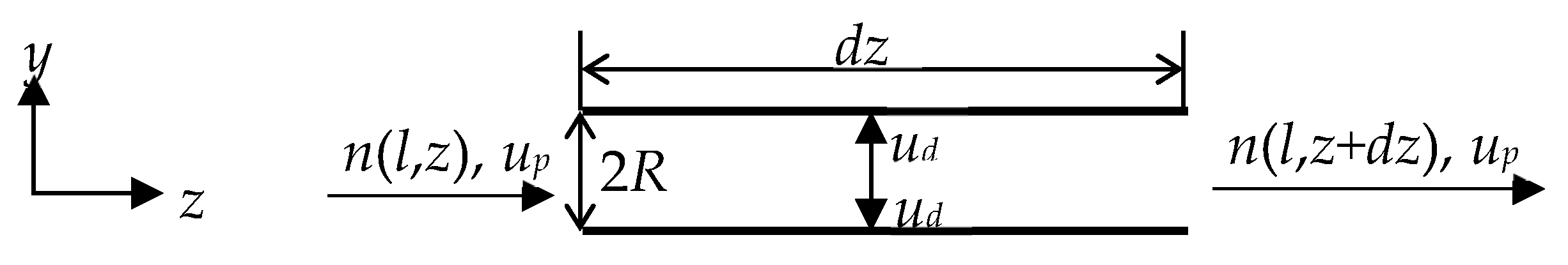
2.1. Geometry, Meshing, and Physical Properties

The geometry used in this study to determine the deposition constant was a horizontal pipe of a length and diameter of 10 m and 0.5 m, respectively. The inlet velocity profile of the flow to the pipe was extracted from a fully developed flow simulation in a 60 m long pipe. The purpose of doing so is to ensure that the flow entering the 10 m long pipe is already fully developed. This is to reduce the mesh element count thus the computational demand but still maintain a turbulent flow in the pipe from the inlet.

The geometry was divided into small control volumes with a hexahedral shape along the axial direction. The radial direction was meshed with an inflation method where the first height of the cell was entered with a known number of layers and a growth rate. This is to account for the near-wall region to capture the change in flow field variables. A mesh size sensitivity analysis for a 60 m long pipe was carried out for the radial and axial directions. By analysing the mean velocity magnitude for both directions, the optimum mesh size can be identified. This is shown in Figures 5–8 in the Results and Discussion Section. The identified optimum mesh size is used in the DPM simulation for a 10 m pipe. It was found that for radial direction a first layer of 1 × 10⁻⁴ m and 1.3 growth factor with 20 layers obtain the optimal mesh, and the size of the cells in the axial direction was 0.05 m.

The above was carried out using Ansys Fluent.

Table 1. Physical properties of the continuous and dispersed phases.

	ρ (kg m−3)	μ (Pa s)	l (μm)
Continuous phase (liquid)	866	0.0012
Dispersed phase (solids)	1200		1–200

shows the physical properties of the continuum and dispersed phases for DPM simulation [24].

2.2. Deposition Constant and Velocity

The deposition constant was determined by dividing the 10 m long pipe into 5 sections as shown in Figure 2a, and the mesh configurations are shown in Figure 2b.

Taking a differential unit of a section from Figure 2a, Figure 3 depicts the particles flowing through this unit by considering deposition.

In Figure 3, n(l,z) (m⁻⁴) is the number density function of the particles of size l at location z; u_p (m s⁻¹) is the average axial velocity of particles. u_d (m s⁻¹) is the deposition velocity of particles of size l in radial direction at location z and R (m) is the radius of the pipe.

n(l,z) is defined based on the number density of particles of size l, N(l,z) (m⁻³). The number density of particles of size l means the number of particles of size l per unit spatial volume at location z. n(l,z) is now written as

$$n\left(l,z\right)=dN(l,z)/dl$$

(1)

The deposition flux J_d(l) (m⁻² m⁻¹ s⁻¹) of particles of size l in this unit in terms of deposition velocity is

$$J_d\left(l,z\right)=u_{d}n(l,z)$$

(2)

This flux can also be calculated by the change in particle number density function:

$$J_d\left(l,z\right)=u_p\left[n\left(l,z+dz\right)-n\left(l,z\right)\right]$$

(3)

Combining Equations (2) and (3), the deposition rate of particles of size l across the axial length of dz is

$$u_p\pi R^2\left[n\left(l,z+dz\right)-n\left(l,z\right)\right]=u_{d}n(l,z)\times 2\pi Rdz$$

(4)

Rearranging Equation (4) yields

$${\displaystyle \frac{n\left(l,z+dz\right)-n\left(l,z\right)}{dz}}={\displaystyle \frac{{2u}_d}{u_{p}R}}n(l,z)$$

(5)

Letting $dz\to 0$ and

$$D={\displaystyle \frac{{2u}_d}{u_{p}R}}$$

(6)

Equation (6) now becomes

$${\displaystyle \frac{dn\left(l,z\right)}{dz}}=-Dn(l,z)$$

(7)

Note, the negative sign on the righthand side of Equation (7) is due to dn(l,z) < 0 attributed to deposition. Equation (7) is the steady-state PBE for deposition only and D (m⁻¹) is the deposition constant, which is interpreted as the number of deposit particles per unit metre length of the pipe in the axial direction.

According to Equation (6), the deposition constant D is inversely proportional to the average particle velocity u_p in the axial direction and the radius R of the pipe in which particles are flowing.

Equation (7) can be discretised to

$${\displaystyle \frac{\mathsf{\Delta }n(l,z)}{\mathsf{\Delta }z}}=-Dn(l,z)$$

(8)

$$D={\displaystyle \frac{-\mathsf{\Delta }n(l,z)}{\mathsf{\Delta }z}}\times {\displaystyle \frac{1}{n(l,z)}}$$

(9)

With DPM providing the concentration information for the sections shown in Figure 2a, Equation (9) indicates that D can be calculated by this discretised form for each of the sections for different particle sizes.

Due to the fact that the deposition constant D can be determined in such a way, from Equation (6), the deposition velocity u_d can be written as

$$u_d={\displaystyle \frac{u_{p}RD}{2}}$$

(10)

Equation (10) suggests that for a given deposition constant, the deposition velocity u_d is proportional to the average axial particle velocity u_p and the pipe radius.

2.3. The Average Particle Velocity in Axial Direction and the Peclet Number in Radial Direction

2.3.1. The Average Particle Velocity in Axial Direction

The average axial velocity of the particles u_p differs from the fluid velocity u_f by the so-called slip velocity u_slip = u_p − u_f. u_slip (m s⁻¹) in horizonal pipe flow is primarily attributed to the balance between the drag force and the buoyancy force acting on particles. Gravity is not considered in this scenario for (1) it only acts on vertical direction and (2) it primarily contributes to sedimentation rather than deposition—sedimentation is only a concentration redistribution and not permanent, but deposition is permanent. Also, the process under consideration is in turbulent flow, so the particles are regarded as uniformly distributed at the same axial location.

The drag force depends on the drag coefficient C_d. There are many empirical models [25,26,27] available for C_d for low to moderate Reynolds numbers (<1000) of particles based on the slip velocity (Re_p = ρ_f u_slip l/μ_f, where ρ_f (kg m⁻³) and μ_f (Pa s) are density and viscosity of the continuous phase, respectively). In terms of applicability, those models are within a few percent of difference from each other. In the case of rarefaction solid–liquid flow (1.0 vol% dispersed particles in this study), the Schiller and Naumann model [27] (C_d = 24(1 + 0.15 Re_p^0.687)/Re_p) was used.

It was also believed that the Stokes number of particles was considered low in the flow. For instance, taking the largest particle size 200 μm and other properties shown in Table 1, the Stokes number (St = τ_p/τ_f, where τ_p (s) and τ_f (s) are particle relaxation time and fluid characteristic time, respectively) can be calculated. According to τ_p = ρ_pl² /18μ = 1200 (2 × 10⁻⁶)²/(18 × 0.0012) = 0.0022 (s) and τ_f = 2R/u_f = 0.5/1 = 0.5 (s) (let the fluid velocity be 1 m s⁻¹), so St = 0.0022/0.5 = 0.0044 << 1, this suggests that the 200 μm particles tend to flow with the fluid stream. So, with smaller particles and larger fluid velocity, this phenomenon would be more prominent.

With C_d = 24(1 + 0.15 Re_p^0.687)/Re_p, the balance between the buoyancy and the drag exerted on particles results in

$$1+{\left({\displaystyle \frac{{\rho }_{f}l}{\mu }}\right)}^{0.687}{u_{slip}}^{0.687}={\displaystyle \frac{{\rho }_{f}g{l}^2}{18\mu }}{u_{slip}}^{-1}$$

(11)

Equation (11) is non-algebraic, so its analytical solution cannot be found. Using trial and error, u_slip can still be worked out numerically and its detail is given in Section 3.2. A fit to the u_slip data is given by Equation (12).

$$u_{slip}={\displaystyle \frac{{\rho }_{f}g}{18{\mu }_f}}{l}^{2.09}$$

(12)

where $g$ (m s⁻²) is the gravitational acceleration.

$$u_p=u_f{-u}_{slip}=u_f-{\displaystyle \frac{{\rho }_{f}g}{18{\mu }_f}}{l}^{2.09}$$

(13)

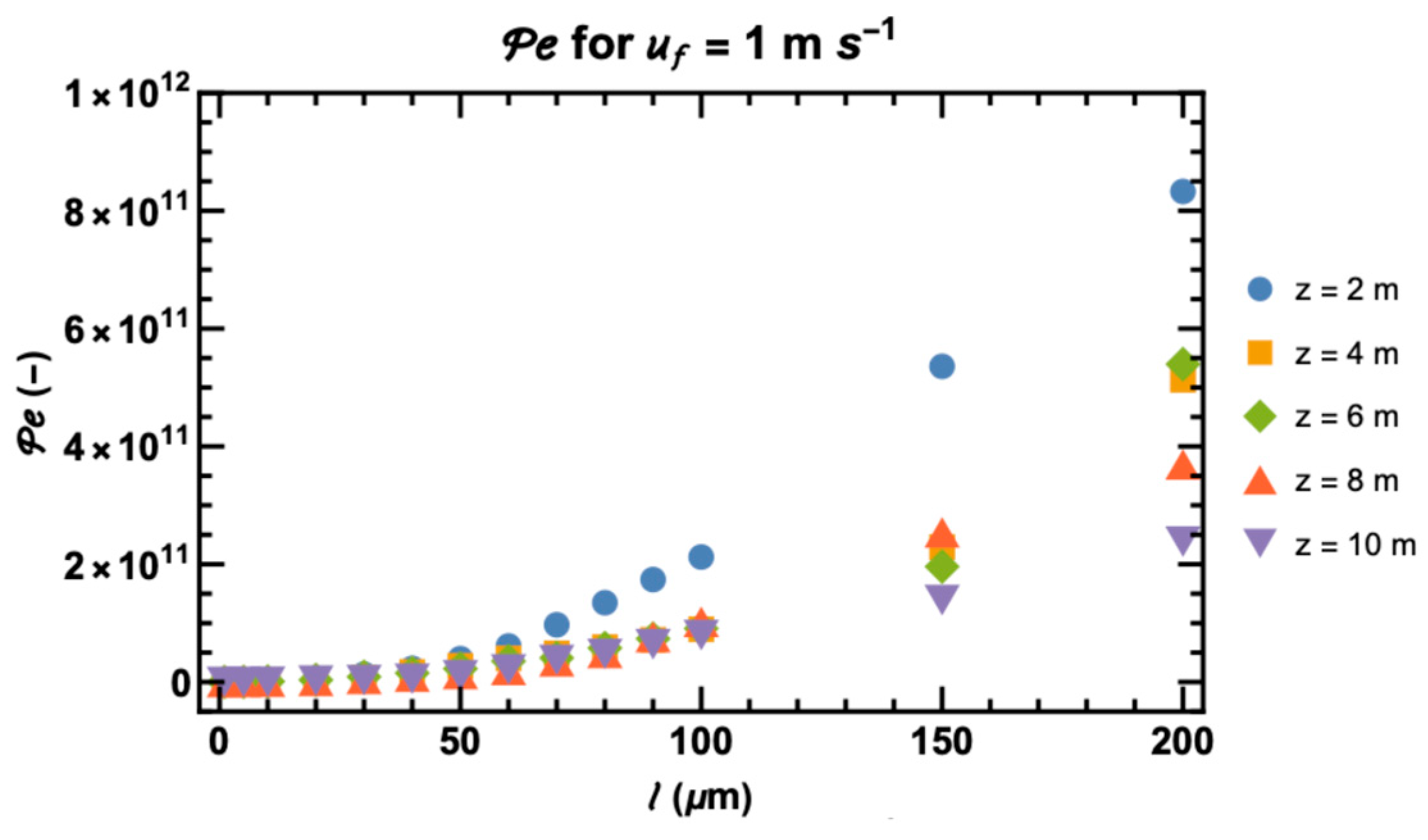
2.3.2. The Peclet Number of Particles in Radial Direction

The Peclet number (Pe) can be used to measure the relative importance of advection to diffusion in a mass transfer process. As discussed in Section 2.3.1, in the axial direction, the Stokes number is well below 1 for the largest particle size and smallest fluid velocity given in this study. There is no doubt that the transport of particles in the axial direction is made by the advection of the flow, the diffusion of particles in the flow in the axial direction is negligible.

Take a sample calculation for the smallest particles of 1 μm in diameter in the fluid velocity of 1 m s⁻¹, with the properties given in Table 1, $Pe={2u}_{f}R/\mathbb{D}$, where $\mathbb{D}$ (m² s⁻¹) is the particle diffusivity, and calculated by $kT/3\pi {\mu }_{f}l$, where k is the Boltzmann constant (1.38 × 10⁻²³ J K⁻¹) and T is the thermal temperature (assumed 298 K). $\mathbb{D}=3.64\times {10}^{-13}$ $Pe=2\times 1\times {\displaystyle \frac{0.25}{3.64}}\times {10}^{-13}=1.38\times {10}^{12}\gg 1$. This suggests that particles in the axial direction are transported by the flow of the continuous phase.

However, in the radial direction in which particles deposit, $Pe=u_{d}l/\mathbb{D}$. A detailed discussion in Section 3.2 is given to show the calculated Pe numbers on how they are depending on the particle size for different pipe locations.

2.4. The Population Balance Equations

In this study, two types of PBEs are developed to model the deposition of particles: a steady-state PBE for the particles in the flow in a pipe and an unsteady-state PBE for the particles depositing on the internal wall of the pipe. The first PBE incorporates deposition with aggregation. This is due to the fact that it is inevitable that aggregation of particles will take place in such a shear-induced flow as first established by Smoluchowski [28] and later further studied by Mumtaz and Hounslow [29] and Liew et al. [30]. The second PBE is for the particles depositing on the internal pipe wall and this is caused by the particle deposition velocity.

2.4.1. The PBE for Particles in Flow

The PBE for particles in flow for simultaneous aggregation and deposition is written as

$${\displaystyle \frac{\partial n\left(l,z\right)}{\partial z}}=-Dn\left(l,z\right)+{\displaystyle \frac{l}{2}}{\int }_0^l{\displaystyle \frac{1}{u_p}}{\displaystyle \frac{\beta \left({\left(l^3-x^3\right)}^{\frac{1}{3}},x,z\right)n\left({\left(l^3-x^3\right)}^{\frac{1}{3}},z\right)n\left(x,z\right)}{{\left(l^3-x^3\right)}^{2/3}}}\mathrm{d}x-n(l,z){\int }_0^{\mathrm{\infty }}{\displaystyle \frac{\beta (l,x,z)}{u_p}}n(x,z)\mathrm{d}x$$

(14)

where x (m) denotes the diameter of particles. The lefthand of Equation (14) is the advection term describing the change in the number density function of particles of size l in the axial direction due to bulk flow. On the righthand side of Equation (14), the first term describes the “death” of particles of size l due to deposition; the second and third term are the “birth” and “death” terms attributed to aggregation, respectively. β (m³ s⁻¹)is the aggregation kernel [31].

For shear-induced aggregation, according to Smoluchowski [28], β is expressed as

$$\beta ={\displaystyle \frac{\dot{\gamma }}{6}}{(l+x)}^3$$

(15)

where l (m) and x (m) are the diameters of two colliding particles, respectively. $\dot{\gamma }$ (s⁻¹) is the shear rate, for a turbulent pipe flow, $\dot{\gamma }$ can be approximated to

$$\dot{\gamma }={\displaystyle \frac{4Q}{\pi R^3}}$$

(16)

where Q (m³ s⁻¹) is the volumetric flow rate of the total flow in the pipe. However, it must be mentioned that $\beta$ was originally derived by Smoluchowski to describe the total number of particle collisions; nevertheless, not all collisions lead to aggregation, so an aggregation efficiency ψ [29,32,33]—sometimes called collision success factor [34,35]—should be applied to Equation (15). With Equation (16) and u_f = Q/πR², we have

$$\beta =\psi {\displaystyle \frac{2Q}{3\pi R^3}}{(l+x)}^3=\psi {\displaystyle \frac{2u_f}{3R}}{(l+x)}^3$$

(17)

According to Liu [34], in suspensions, ψ depends on the ratio of critical relative kinetic energy to the overall average kinetic energy of the particles and takes this form [35]:

$$\psi =(1+{\displaystyle \frac{{{\theta }_c}^{*}}{{\theta }_s}})\mathrm{e}\mathrm{x}\mathrm{p}(-{\displaystyle \frac{{{\theta }_c}^{*}}{{\theta }_s}})$$

(18)

where θ_c^* (J) is the critical relative kinetic energy of two colliding particles that describe the balance between attraction and repulsion and θ_s (J) is the overall average kinetic energy of the particles in the system.

While θ_s depends on the average particle velocity, in the case of this study, it is u_p; however, to work out θ_c^*, a thorough study of the particle interactions in liquids at close ranges would have to be made. This certainly is beyond the scope of this article and would make the focus away from deposition.

Nevertheless, it was found that in either granulation processes [36] or aggregation in nanosuspension systems [35], the typical value of ψ was in the order of 10⁻², while for a nanosuspension system, it was suggested [35] that a value of ψ around 10⁻⁶ can be considered as making a stable system (aggregation-free or negligible). Here, a value of 10⁻⁴ for ψ is taken into our PBM computation.

2.4.2. The PBE for Particles Depositing on the Pipe Wall

The PBE for particles depositing on the pipe wall can be written as

$${\displaystyle \frac{\partial n_w\left(t,l,z\right)}{\partial t}}=u_{d}Dn(l,z)$$

(19)

where n_w(t,l,z) (m⁻⁴) is the number density function of particles of size l depositing on the surfaces of the internal pipe wall. It has similar definition to n(l,z), as given by Equation (1), but the number density would refer to the particles depositing on the wall. The rationale that Equation (19) came into being is that in any axial location of the pipe, the number of particles depositing out of the flow must be depositing at the same location on the wall. Thus, according to Equation (6), Equation (19) can be rewritten as

$${\displaystyle \frac{\partial n_w\left(t,l,z\right)}{\partial t}}={\displaystyle \frac{2{u_d}^2}{u_{p}R}}n\left(l,z\right)=D_{w}n\left(l,z\right)$$

(20)

where D_w = 2u_d²/Ru_p (s⁻¹) is the deposition rate constant of particles on the wall. Equation (20) is the PBE for particles depositing on the wall. It is clear that Equation (20) takes the solution of n(l,z) from Equation (14) to solve for n_w(t,l,z). It is worth noting that n(l,z) solved in Equation (14) is the number density function of particles of size l at an axial location of z; it is thus true that n_w(t,l,z) solved in Equation (20) is also the number density function of particles of size l depositing on the wall at the same axial location.

It should be pointed out that there is no general analytical solution for Equation (14), its numerical solution for n(l,z) must be sought. The numerical strategy used in this PBM is based on the approach developed by Hounslow et al. [37]. The key feature in this approach is that the progression of two discretised neighbouring volume sizes of the particles is set to be ½, e.g., v_i+1/v_i = 2 or l_i+1/l_i = 2^1/3. This turns the partial differential equations into the ordinary ones while still maintains the overall mass conservation, which made the pursuit of the solutions for Equations (14) and (20) much more straightforward.

2.5. Thickness of the Deposit

The thickness of deposit at a location z is calculated by the 3rd Moment m₃ of the deposit particles on the wall at the same location, that is:

$$m_3(t,z)={\int }_0^{\mathrm{\infty }}{l}^3{n}_w\left(t,l,z\right)dl$$

(21)

Taking the particle shape factor as π/6, the total volume fraction of the particles at time t and location z is πm₃/6. The thickness δ (m) of the deposit at the same time t and location z is then according to this:

$${\displaystyle \frac{[\pi R^2-{\pi \left(R-\delta \right)}^2]dz}{\pi R^{2}dz}}={\displaystyle \frac{\pi m_3}{6}}$$

(22)

As δ should be less than R, solving Equation (22) gives

$$\delta =R\left(1-\sqrt{1-m_3\pi /6}\right)$$

(23)

2.6. The Particle Size Range, Their Initial Distribution, and the Velocity of the Continuous Phase

2.6.1. Size Range of the Particles

The particle size range used in the DPM simulation was from 1 μm to 200 μm, as shown in

Table 2. Sizes of particles used in DPM simulation.

l (μm)	1	5	10	20	30	40	50
	60	70	80	90	100	150	200

. These particle sizes are used to determine the deposition constants.

2.6.2. The Initial Particle Size Distribution

For PBM, the initial PSD was given in a normal distribution as shown in Figure 4. The total volume fraction of the particles at the inlet of the pipe in the flow was given to be 1%.

2.6.3. Velocity of the Continuous Phase, Length of the Pipe, and Time for PBM

The average axial velocities of the continuous phase at the inlet of the pipe are set to be 1 m s⁻¹, 3 m s⁻¹, 5 m s⁻¹, and 10 m s⁻¹ respectively for both DPM and PBM. Their corresponding Reynolds numbers are 3.61 × 10⁵, 1.08 × 10⁶, 1.80 × 10⁶, and 3.61 × 10⁶. So, the continuous flow in the pipe is well in the turbulent region. In addition, the length of the pipe and the time for the PBM are set to be 1000 m and 3600 s, respectively, to observe the general occurrence of deposition and the development of the thickness of the deposit.

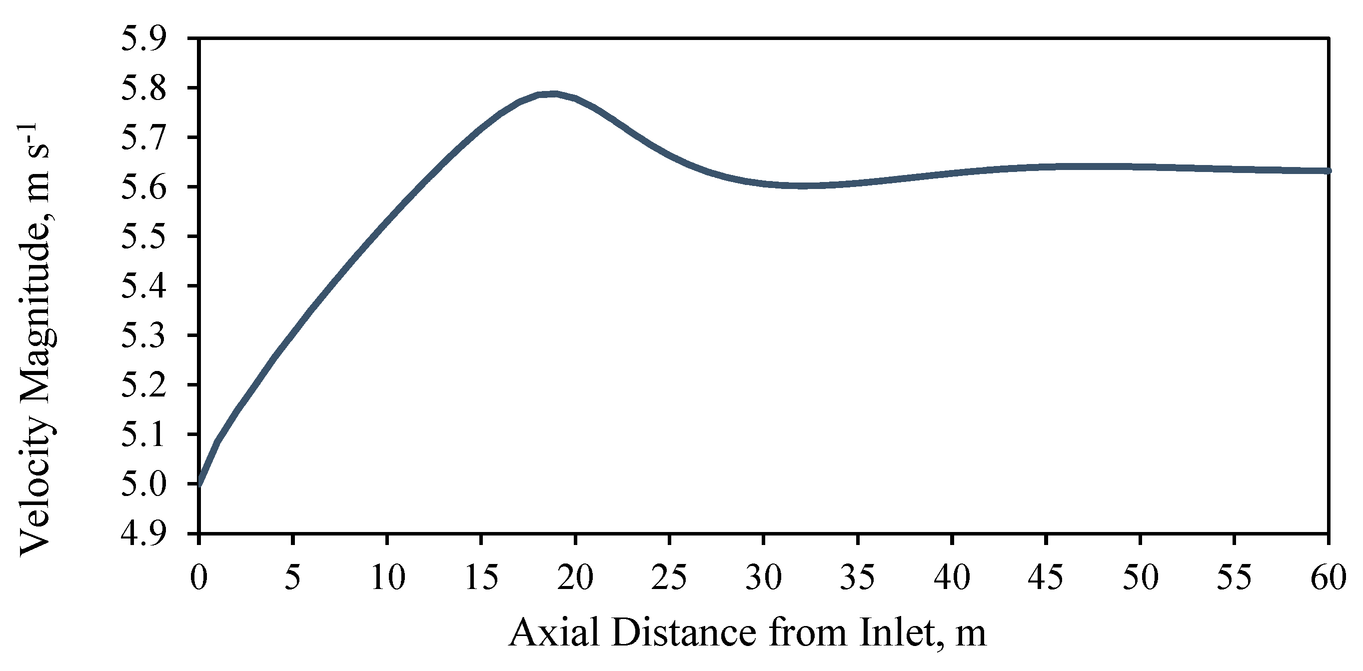
3. Results and Discussion

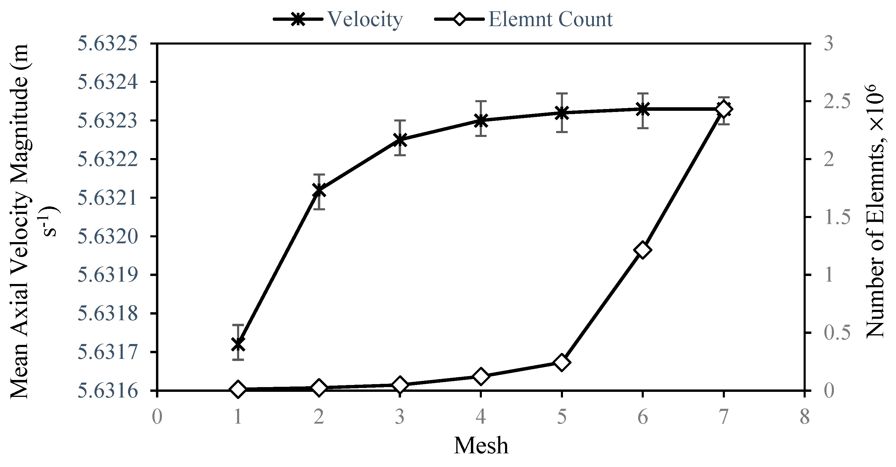
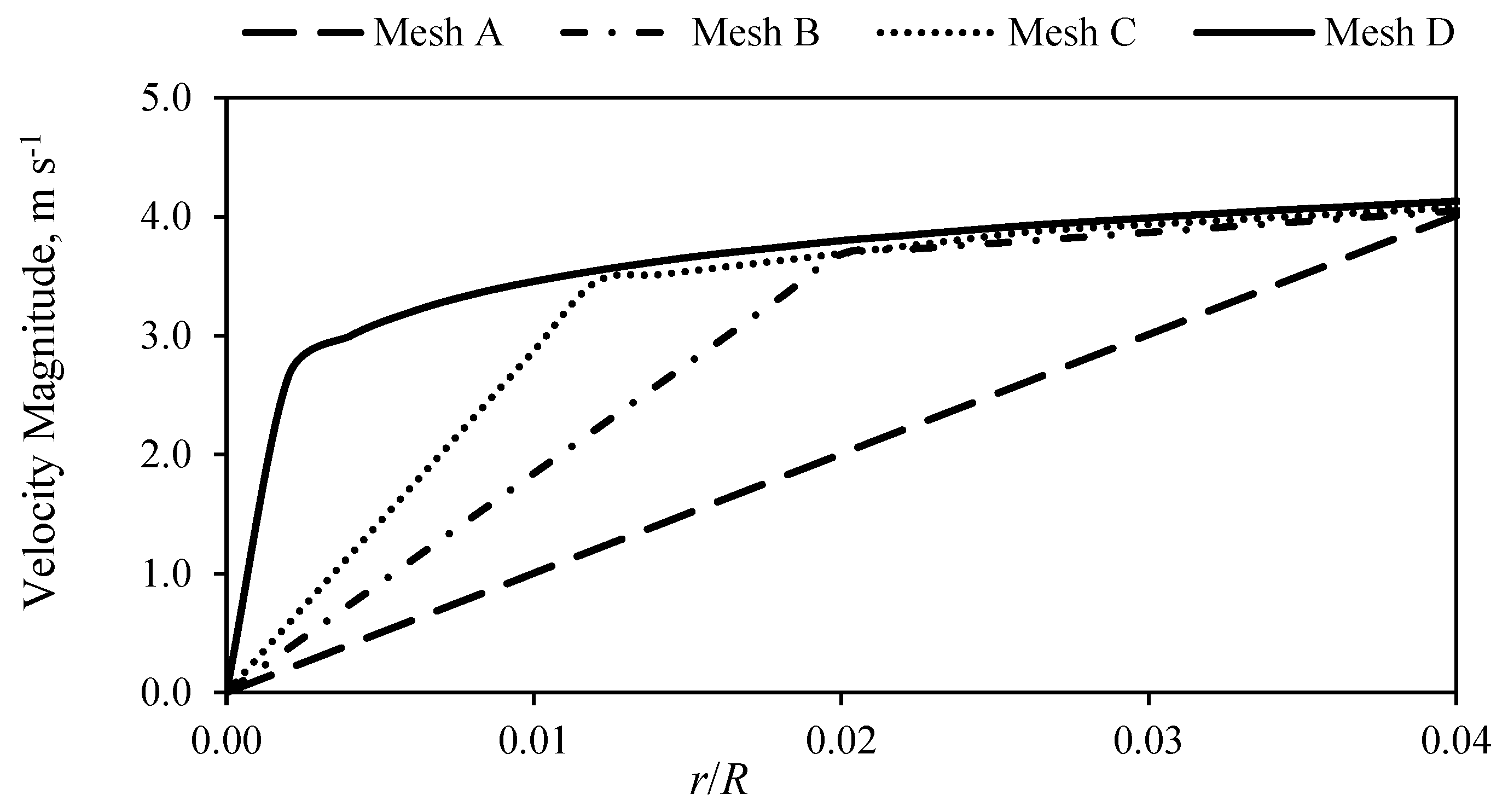
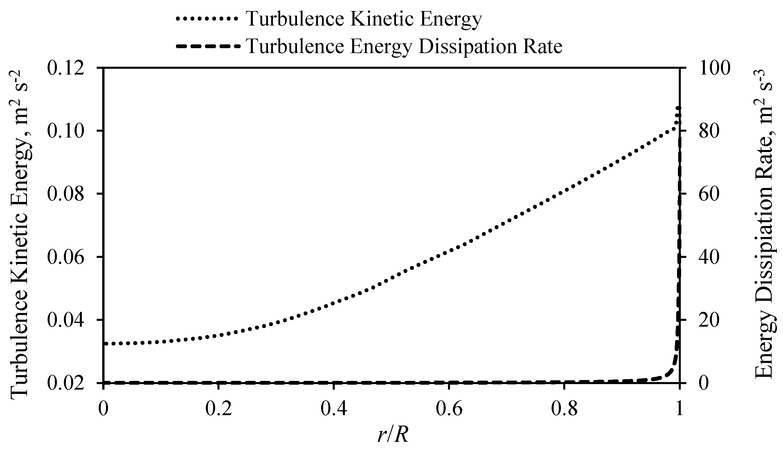
3.1. Mesh Sensitivity

To capture the velocity profile for fully developed flow, the simulation was first carried out in a pipe of 60 m long. When a steady velocity profile in the axial direction was observed, the outlet flow property profiles were extracted. In this case the steady axial velocity profile appeared after axial length of 30 m from the inlet, indicating that a steady flow was achieved, as depicted in Figure 5. The properties of the outlet, (e.g., velocity components, turbulence kinetic energy k, and dissipation rate ε) were then exported and inserted as the boundary conditions at the inlet of the 10 m long pipe to simulate and determine the deposition constant.

Axial mesh refinement was also carried out over the 10 m pipe. The refinement was implemented with elements of different sizes as classified by numbers 1–7, as shown in Figure 6.

As shown in Figure 6, the mean velocity magnitude did not change significantly after Mesh 4, while the number of elements increased exponentially. Mesh 5 was the optimal mesh configuration for axial direction partitioning, with an element count of 243200. Similarly, the mesh was refined in the radial direction to accommodate the rapid change in velocity in the near-wall region, as seen in Figure 7.

As seen from Figure 7, Mesh A to C show either linear or sectional linear velocity profiles, which indicate that the boundary layer was not properly represented. Mesh D was a better non-linear velocity profile representation. Figure 8 shows the turbulence kinetic energy, k, and the turbulence energy dissipation rate, ε, from the simulation based on axial Mesh 5 and radial Mesh D.

As seen from Figure 8, the two properties are higher at the wall, as both were affected by the presence of the boundary.

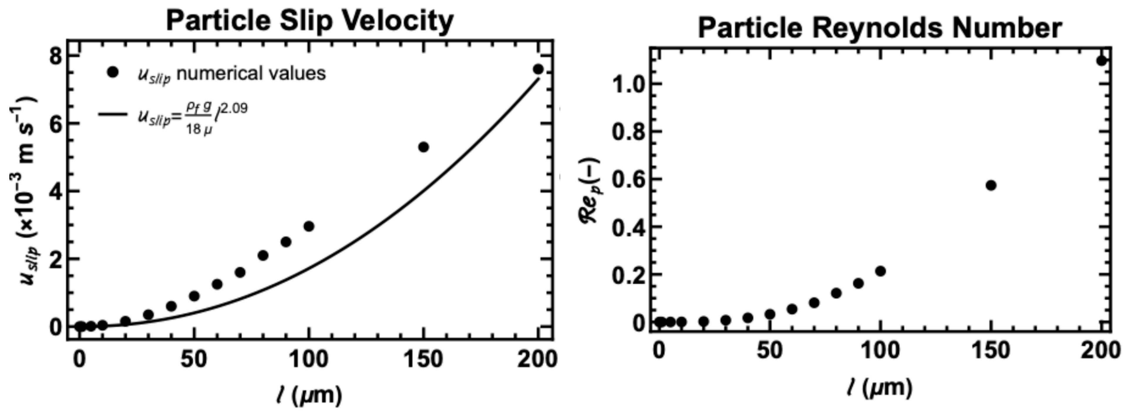
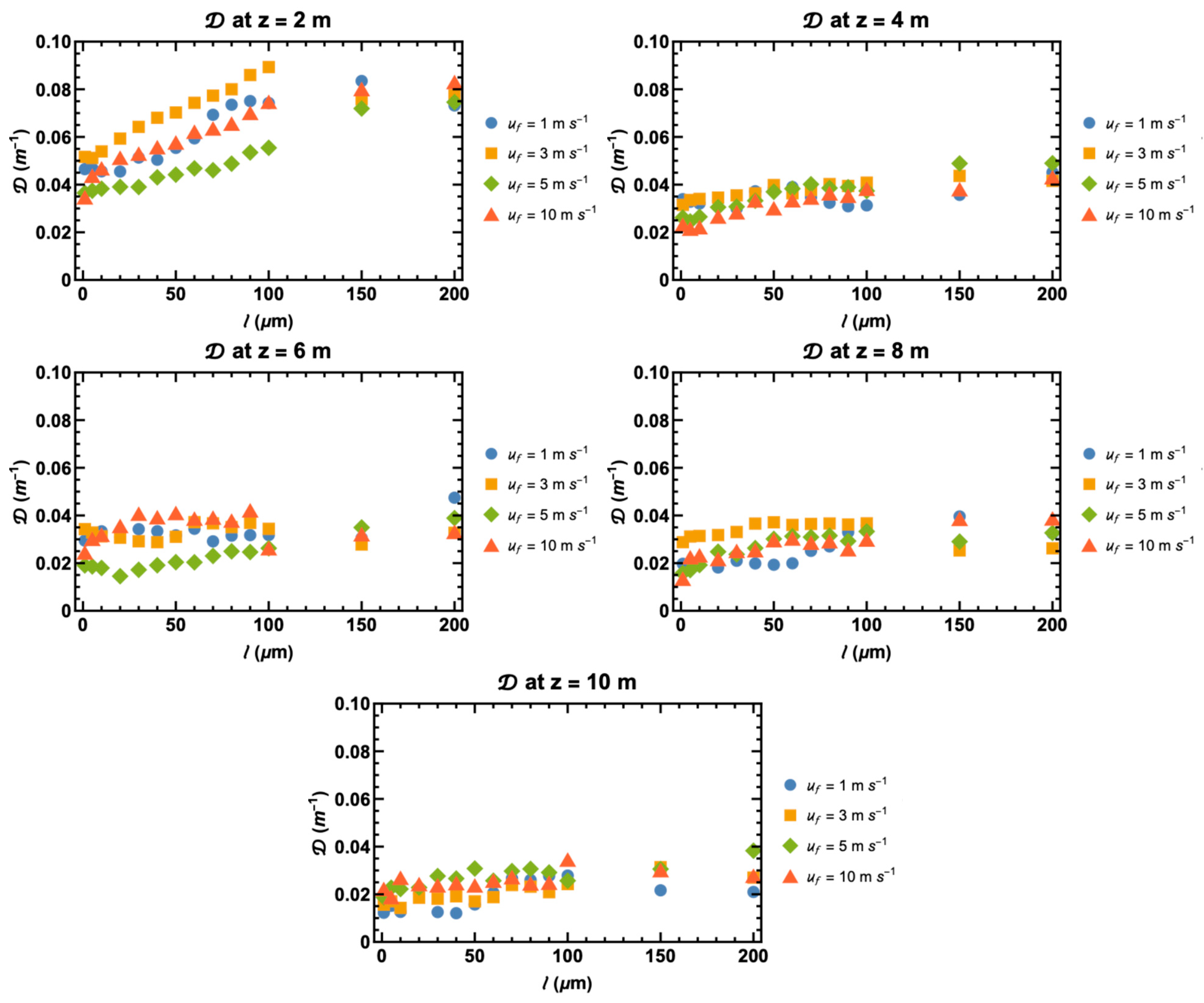
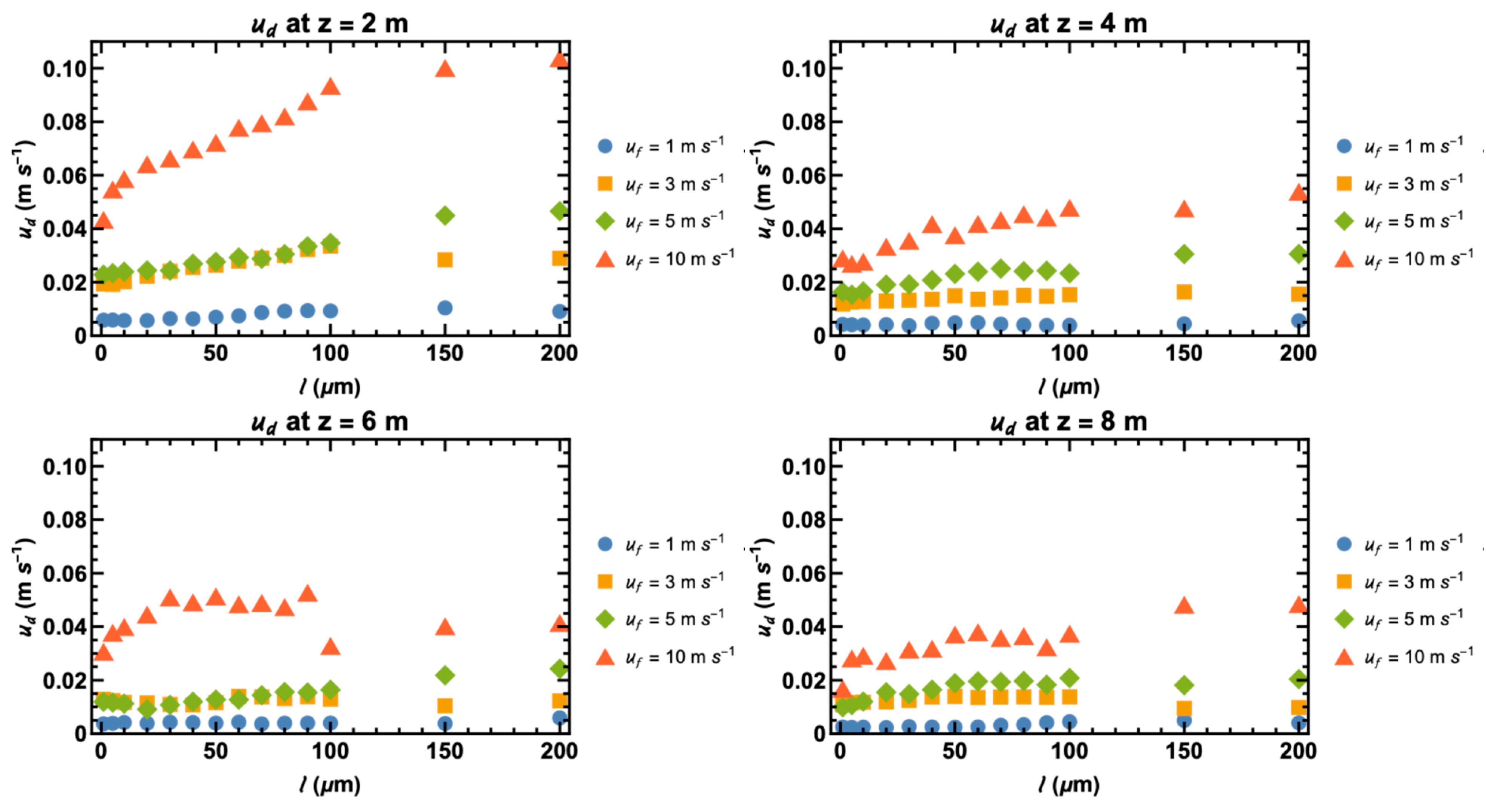
3.2. Slip Velocity, Deposition Constant, and Deposition Velocity

Figure 9 shows the slip velocity and Reynolds number of the particles in the axial direction.

As can be seen from Figure 9, for particles of 200 μm in diameter, the slip velocity was approximately 0.0076 m s⁻¹. With a continuous flow of 1 m s⁻¹, this counts about 0.76% of the velocity of the continuous phase. As also seen from the particle Reynolds number plot, they are all very well below 1000.

The deposition constant calculated based on Equation (9) is shown in Figure 10 for different flow velocities. These results were obtained from DPM for a 10 m long pipe with fully developed flow velocity profile at the inlet. The average axial flow velocities at the inlet were 1 m s⁻¹, 3 m s⁻¹, 5 m s⁻¹, and 10 m s⁻¹, respectively.

As can be seen from Figure 10, for each of the flow velocities, the deposition constant generally increases with the increase in particle size. In terms of the location of the pipe, it decreases in general along the pipe. It is also worth pointing out that the deposition constant appears to be larger at the near inlet of the pipe.

Figure 11 shows a comparison of the deposition constant at the same location for different flow velocities.

As seen from Figure 11, from the DPM results, the continuous flow velocity does not seem to make a significant difference for deposition constant. Nevertheless, the deposition constant tends to be slightly larger for higher flow velocity, especially at the outlet of the pipe compared to that at the near inlet.

Figure 12 shows the calculated deposition velocity of the particles based on Equation (10) for different flow velocities at different pipe locations.

As can be seen from Figure 12, the deposition velocity at the near inlet of the pipe appears to be generally larger than that along the pipe towards outlet. It also shows that the deposition velocity increases with the particle size. Figure 13 shows the comparison of the deposition velocity at the same location of the pipe but for different flow velocities.

It is clear from Figure 13 that a larger flow velocity results in a larger deposition velocity. This can be explained by Equation (10), as the deposition velocity is proportional to the average particle velocity in the axial direction, and, as shown in Equation (12), the average particle velocity in axial direction increases with the increase in flow velocity. However, it needs to be pointed out that according to Equation (10), the deposition velocity is also proportional to the deposition constant, but as seen from Figure 11, the deposition constant can be said to largely remain level except for that at z = 2 m. Nevertheless, even at z = 2 m, the variation of deposition constants in flow velocity is still quite small compared to the average axial particle velocity changes. This means that the change in average axial particle velocity overperforms the change in deposition constant at the same pipe location, which indicates that particle velocity u_p is the dominating factor in determining u_d in Equation (10).

Figure 14 shows the Peclet number plot for continuous flow velocity 1 m s⁻¹ as it produces the lowest deposition velocity, as shown in Figure 13.

As can be seen from Figure 14, all the Peclet numbers are significantly greater than 1. Even for the smallest particle size 1 μm at location z = 10 m, Pe was calculated to be 3.5 × 10⁶. This suggests that in terms of the transport of particles from the continuous phase to the wall to form the deposit, the mechanism is not due to diffusion; instead, it is still attributed to the advection of the particles in the radial direction. This results from the combined action of the forces in the DPM simulation, as explained in the Introduction Section (the fourth paragraph above Figure 1) of this article.

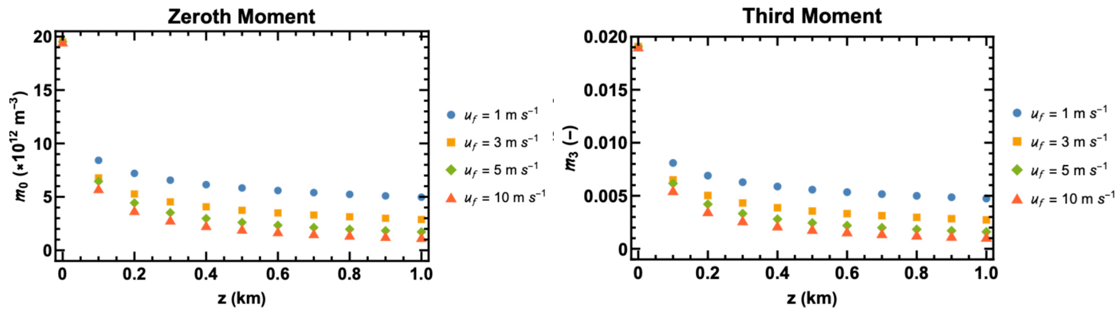
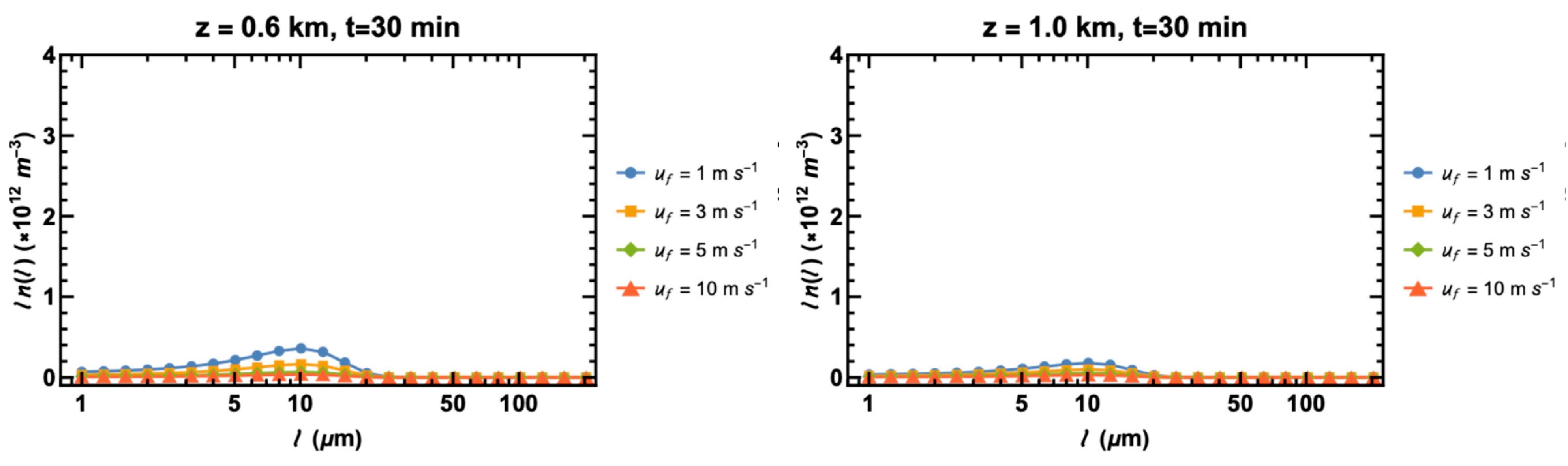
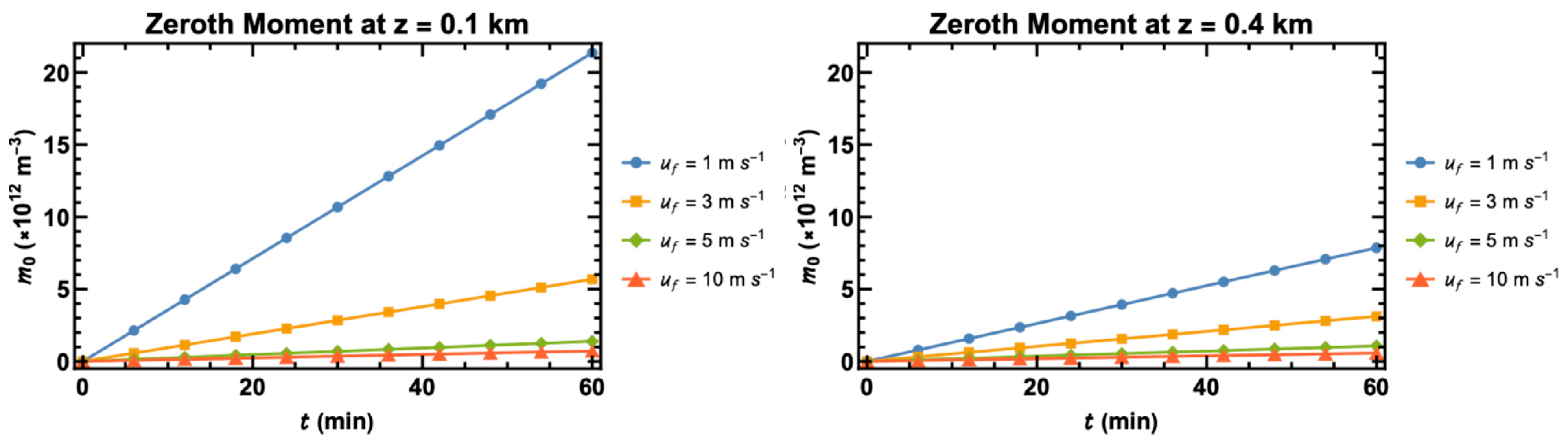
3.3. Size Distribution and Moments of Particles in the Flow

Figure 15 shows the size distribution of the PBM results for the particles flowing in a 1000 m long pipe involving a simultaneous aggregation and deposition for different flow velocities at different pipe locations. These PSDs are the solutions of Equation (14).

It can be seen from Figure 15 that the size distribution becomes lower as the flow velocity increases. This is mainly due to the fact that the deposition constant generally increases with the flow velocity, as shown in Figure 11, and that deposition dominates over aggregation.

Figure 16 compares the 0th Moment ($m_0\left(z\right)={\int }_0^{\mathrm{\infty }}n\left(l,z\right)dl$) and 3rd Moment $m_3\left(z\right)={\int }_0^{\mathrm{\infty }}{l}^{3}n\left(l,z\right)dl$.

Figure 16 confirms what Figure 14 suggests, that is, the total number (m₀) and volume (πm₃/6) of the particles per unit volume in the flow both decrease along the pipe, and the larger the flow velocity, the greater the decrease. Towards outlet of the pipe, both m₀ and m₃ gradually became steady.

3.4. Size Distribution and Moments for Particles on the Internal Pipe Wall

For the particles deposited on the wall, Figure 17 shows how their size distributions change with time at different pipe locations.

It is clear from Figure 17 that the further down the pipe and away from the inlet, the less the deposition. The number of particles deposited on the wall increases with the decrease in continuous flow velocity, which is in agreement with the literature [19,20,23,24]. Figure 18 and Figure 19 further confirm this at a time of 30 and 60 min, respectively.

Figure 20 and Figure 21 show both m₀ and m₃ of the particles how they change with time at different pipe locations and flow velocities.

It is clear from Figure 20 and Figure 21 that both the total number density and volume fraction of the deposit particles on the pipe wall decrease along the pipe as well as with the increase in flow velocity. Both figures also imply that with time proceeding, there will be more deposits on the pipe wall.

3.5. Thickness of the Deposits

Figure 22 shows the calculated thickness of the deposit particles along the pipe for different flow velocities.

As can be seen from Figure 22, lower flow velocity produces more deposits, while compared to u_f = 1 m s⁻¹, the accumulated thickness of the particles deposited on the wall is almost insignificant for u_f = 5 m s⁻¹ and 10 m s⁻¹ for this modelling of 60 min in total.

Take an example of the deposition at the inlet where z = 0: at 60 min, the δ values for u_f = 1 m s⁻¹, 3 m s⁻¹, 5 m s⁻¹, and 10 m s⁻¹ are 3.98 mm, 0.58 mm, 0.1 mm, and 0.05 mm, respectively. As seen, the δ value for u_f = 1 m s⁻¹ is 6.8 times of that for u_f = 3 m s⁻¹, 39.8 times of that for u_f = 5 m s⁻¹, and 79.6 times for u_f = 10 m s⁻¹. This suggests that for a typical setting of the particle and continuous phase properties shown in Table 1 and Table 2, and with a 1 vol% of the particles at the inlet in a pipe of 0.5 m in diameter, a 5 m s⁻¹ continuous phase flow would significantly reduce the deposition of particles especially at the inlet.

It has to be mentioned that while Figure 11 and Figure 13 have indicated that the deposition constant and velocity for particles in the flow largely increase with the increase of the continuous phase flow velocity. The deposit thickness, size distribution, and Moments of the particles that have deposited on the internal pipe wall shown in Figure 18, Figure 19, Figure 20, Figure 21 and Figure 22 are seemingly against this trend. This can be explained by Equation (20), specifically by the bulk constant 2u_d²/u_pR, which is inversely proportional to u_p. As aforementioned that u_p overperforms u_d in the first order and the values of u_d are in the order of 10⁻², in the evaluation of 2u_d²/u_pR, u_p is the dominating factor; this means increasing u_p would decrease 2u_d²/u_pR so as to the number density n_w(t,l,z) of the particles depositing on the wall.

4. Conclusions

Incorporating the DPM and PBM has made the deposition involving aggregation modelling possible for a turbulent particle–liquid flow in a pipe of industrial scale. It was found that the deposition constant and velocity of the particles in the flow increase with the increase in flow velocity of the continuous phase. However, the deposition of the particles on the wall goes otherwise—the larger the continuous flow velocity, the less the deposit. It was also found that the deposition mainly takes place at the inlet of the pipe then decreases significantly towards the outlet of the pipe. In a setting of the solid and liquid phase properties, pipe size, and flow conditions similar to what this article has studied, a 5 m s⁻¹ continuous flow velocity would significantly reduce the particle deposition at the inlet as well as along the pipe towards outlet. The calculated Pe numbers suggest that the deposition of particles in such a turbulent flow is a result of advection rather than diffusion.

The method presented in this article has provided a generally useful approach to model industrial particle deposition processes that involve particle interaction mechanisms such as aggregation as none of DPM and PBM can undertake it alone. DPM feeds deposition constants to PBM then PBM generates PSDs for steady-state and unsteady-state processes. As one may see this as an advantage of this approach, it may just prove to be the limitation of this approach: if one fails then the other would not work correctly. In an event that the generated PSD outcome does not meet reality, it is likely it is the DPM that may have failed. This is because the PBE is a single equation for groups of particles and its solution procedures are much less dependent on computational settings. But the Lagrangian method based DPM has to solve all the conservation equations for individual particles. This places it at a much higher risk of producing unrealistic or even incorrect results because of its demanding on computational power for converging procedures and accuracy attainment.

Nevertheless, it has to be pointed out that the whole approach is robust, as there is no assumption across the coupling. In terms of solution procedure, there is no convergence requirement for PBM, as all the partial differential equations are transformed into ordinary differential equations. However, there is a convergency requirement for the DPM solution procedure, as its validity depends on the accuracy residual. This procedure difference in seeking solution has resulted in a significant difference in computational time. For PBM, obtaining the solution takes only a matter of seconds, while for DPM, it requires hours of running on a modern desktop computer.

References

1. Fissan, H.; Opiolka, S. Particle Deposition in High Capacity Preseparators. Part. Part. Syst. Charact. 1985, 2, 133–136. [Google Scholar] [CrossRef]
2. Elimelech, M.; Gregory, J.; Jia, X.; Williams, R.A.F. (Eds.) Particle Deposition and Aggregation: Measurement, Modelling and Simulation; Butterworth-Heinemann: Oxford, UK, 1998. [Google Scholar]
3. Pantusheva, M.; Mitkov, R.; Hristov, P.O.; Petrova-Antonova, D. Air Pollution Dispersion Modelling in Urban Environment Using CFD: A Systematic Review. Atmosphere 2022, 13, 1640. [Google Scholar] [CrossRef]
4. Longest, P.W.; Bass, K.; Dutta, R.; Rani, V.; Thomas, M.L.; El-Achwah, A.; Hindle, M. Use of computational fluid dynamics deposition modeling in respiratory drug delivery. Expert Opin. Drug Deliv. 2019, 16, 7–26. [Google Scholar] [CrossRef]
5. Ding, Y.; Chen, T.; Tian, H.; Shu, G.; Zhang, H. Experimental and numerical investigation of soot deposition on exhaust heat exchanger tube banks. Therm. Sci. Eng. Prog. 2023, 39, 101699. [Google Scholar] [CrossRef]
6. Song, J.; Wei, Y.; Sun, G.; Chen, J. Experimental and CFD study of particle deposition on the outer surface of vortex finder of a cyclone separator. Chem. Eng. J. 2017, 309, 249–262. [Google Scholar] [CrossRef]
7. Li, Y.; Liu, D.; Cui, B.; Lin, Z.; Zheng, Y.; Ishnazarov, O. Studying particle transport characteristics in centrifugal pumps under external vibration using CFD-DEM simulation. Ocean Eng. 2024, 301, 117538. [Google Scholar] [CrossRef]
8. Tandon, P.; Adewumi, M.A. Particle deposition from turbulent flow in a pipe. J. Aerosol Sci. 1998, 29, 141–156. [Google Scholar] [CrossRef]
9. Buenrostro-Gonzalez, E.; Lira-Galeana, C.; Gil-Villegas, A.; Wu, J. Asphaltene precipitation in crude oils: Theory and experiments. AIChE J. 2004, 50, 2552–2570. [Google Scholar] [CrossRef]
10. Jia, W.; Okuno, R. Modeling of asphaltene and water associations in petroleum reservoir fluids using cubic-plus-association EOS. AIChE J. 2018, 64, 3429–3442. [Google Scholar] [CrossRef]
11. Vegendla, S.N.P.; Heynderickx, G.J.; Marin, G.B. Comparison of Eulerian–Lagrangian and Eulerian–Eulerian method for dilute gas–solid flow with side inlet. Comput. Chem. Eng. 2011, 35, 1192–1199. [Google Scholar] [CrossRef]
12. Emani, S.; Ramasamy, M.; Shaari, K.Z.K. Discrete phase-CFD simulations of asphaltenes particles deposition from crude oil in shell and tube heat exchangers. Appl. Therm. Eng. 2019, 149, 105–118. [Google Scholar] [CrossRef]
13. Bayat, M.; Aminian, J.; Bazmi, M.; Shahhosseini, S.; Sharifi, K. CFD modeling of fouling in crude oil pre-heaters. Energy Convers. Manag. 2012, 64, 344–350. [Google Scholar] [CrossRef]
14. Han, Z.; Xu, Z.; Yu, X. CFD modeling for prediction of particulate fouling of heat transfer surface in turbulent flow. Int. J. Heat Mass Transf. 2019, 144, 118428. [Google Scholar] [CrossRef]
15. Zhang, J.; Li, A. CFD simulation of particle deposition in a horizontal turbulent duct flow. Chem. Eng. Res. Des. 2008, 86, 95–106. [Google Scholar] [CrossRef]
16. Chaumeil, F.; Crapper, M. Using the DEM-CFD method to predict Brownian particle deposition in a constricted tube. Particuology 2014, 15, 94–106. [Google Scholar] [CrossRef]
17. Akermann, K.; Renze, P. Numerical study of turbulent heat transfer and particle deposition in enhanced pipes with helical roughness. Int. J. Multiph. Flow 2024, 176, 104827. [Google Scholar] [CrossRef]
18. Akter, F.; Saha, S. Deposition of aerosol particles and characteristics of turbulent flow inside wavy pipe using Eulerian-Lagrangian approach. Chem. Eng. Process.—Process Intensif. 2024, 205, 109971. [Google Scholar] [CrossRef]
19. Azimifar, M.; Moradian, A.; Jafarian, A. A numerical investigation on the dynamics of particle deposition and fouling on a vertical falling film pipe. J. Water Process Eng. 2024, 66, 105990. [Google Scholar] [CrossRef]
20. Balakin, B.V.; Hoffmann, A.C.; Kosinski, P. Experimental study and computational fluid dynamics modeling of deposition of hydrate particles in a pipeline with turbulent water flow. Chem. Eng. Sci. 2011, 66, 755–765. [Google Scholar] [CrossRef]
21. Haghshenasfard, M.; Hooman, K. CFD modeling of asphaltene deposition rate from crude oil. J. Pet. Sci. Eng. 2015, 128, 24–32. [Google Scholar] [CrossRef]
22. Valus, M.G.; Fontoura, D.V.R.; Serfaty, R.; Nunhez, J.R. Computational fluid dynamic model for the estimation of coke formation and gas generation inside petrochemical furnace pipes with the use of a kinetic net. Can. J. Chem. Eng. 2017, 95, 2286–2292. [Google Scholar] [CrossRef]
23. Eskin, D.; Ratulowski, J.; Akbarzadeh, K.; Pan, S. Modelling asphaltene deposition in turbulent pipeline flows. Can. J. Chem. Eng. 2011, 89, 421–441. [Google Scholar] [CrossRef]
24. Seyyedbagheri, H.; Mirzayi, B. CFD modeling of high inertia asphaltene aggregates deposition in 3D turbulent oil production wells. J. Pet. Sci. Eng. 2017, 150, 257–264. [Google Scholar] [CrossRef]
25. Boyd, F.E.; Joseph, W.W.; Earl, E.S. Dynamics of falling raindrops. Eur. J. Phys. 2001, 22, 113. [Google Scholar] [CrossRef]
26. Putnam, A. Integratable Form of Droplet Drag Coefficient. ARS J. 1961, 31, 1467–1468. [Google Scholar]
27. Shiller, L.; Naumann, A. A Drag Coefficient Correlation1935. Z. Des Ver. Dtsch. Ingenieure 1935, 77, 318–320. [Google Scholar]
28. Smoluchowski, M.V. Drei Vortrage uber Diffusion, Brownsche Bewegung und Koagulation von Kolloidteilchen. Z. Fur Phys. 1916, 17, 557–585. [Google Scholar]
29. Mumtaz, H.S.; Hounslow, M.J. Aggregation during precipitation from solution: An experimental investigation using Poiseuille flow. Chem. Eng. Sci. 2000, 55, 5671–5681. [Google Scholar] [CrossRef]
30. Liew, T.L.; Barrick, J.P.; Hounslow, M.J. A Micro-Mechanical Model for the Rate of Aggregation during Precipitation from Solution. Chem. Eng. Technol. 2003, 26, 282–285. [Google Scholar] [CrossRef]
31. Hulburt, H.M.; Katz, S. Some problems in particle technology: A statistical mechanical formulation. Chem. Eng. Sci. 1964, 19, 555–574. [Google Scholar] [CrossRef]
32. Serra, T.; Casamitjana, X. Effect of the shear and volume fraction on the aggregation and breakup of particles. AIChE J. 1998, 44, 1724–1730. [Google Scholar] [CrossRef]
33. Tandon, P.; Diamond, S.L. Hydrodynamic effects and receptor interactions of platelets and their aggregates in linear shear flow. Biophys. J. 1997, 73, 2819–2835. [Google Scholar] [CrossRef]
34. Liu, L. Kinetic theory of aggregation in granular flow. AIChE J. 2011, 57, 3331–3343. [Google Scholar] [CrossRef]
35. Liu, L. Aggregation of silica nanoparticles in an aqueous suspension. AIChE J. 2015, 61, 2136–2146. [Google Scholar] [CrossRef]
36. Liu, L. Effects of aggregation on the kinetic properties of particles in fluidised bed granulation. Powder Technol. 2015, 271, 278–291. [Google Scholar] [CrossRef]
37. Hounslow, M.J.; Ryall, R.L.; Marshall, V.R. A discretized population balance for nucleation, growth, and aggregation. AIChE J. 1988, 34, 1821–1832. [Google Scholar] [CrossRef]
Figure 1. Schematic of coupling DPM and PBM.
Powders 04 00020 g001
Figure 2. (a) Sectioned pipe and (b) mesh configurations (left: radial direction; right: axial direction). Note, the duplicated legends below the graphs are the recreated due to the illegibility of the original ones.
Powders 04 00020 g002
Figure 3. Schematic of particles flowing through a differential unit of a section of the pipe.
Powders 04 00020 g003
Figure 4. The initial particle size distribution.
Powders 04 00020 g004
Figure 5. Velocity magnitude profile in the axial direction.
Powders 04 00020 g005
Figure 6. Mean velocity magnitude in the axial direction versus number of elements for Mesh 1–7 with their corresponding size as 1 m, 0.5 m, 0.25 m, 0.1 m, 0.05 m, 0.01 m, and 0.005 m, respectively.
Powders 04 00020 g006
Figure 7. Velocity magnitude profile in the radial direction for different mesh arrangements. Note, the first mesh size, growth rate, and number of inflation layers for Mesh A to D are 1 × 10⁻² m, 1.2, and 5; 5 × 10⁻³ m, 1.2, and 10; 3 × 10⁻³ m, 1.2, and 10; and 5 × 10⁻⁴ m, 1.2, and 20, correspondingly.
Powders 04 00020 g007
Figure 8. Turbulence kinetic energy and kinetic energy dissipation rate in the radial direction.
Powders 04 00020 g008
Figure 9. The slip velocity of particles in axial direction.
Powders 04 00020 g009
Figure 10. Deposition constants vs. particle size for different flow velocities at different pipe locations.
Powders 04 00020 g010
Figure 11. Comparison of the deposition constants at different locations of the pipe for different flow velocities.
Powders 04 00020 g011
Figure 12. Deposition velocity vs. particle size for different flow velocities at different pipe locations.
Powders 04 00020 g012
Figure 13. Comparison of the deposition velocity at the same pipe location but for different flow velocities.
Powders 04 00020 g013aPowders 04 00020 g013b
Figure 14. Peclet number plot for uf = 1 m s−1 at different pipe locations.
Powders 04 00020 g014
Figure 15. Comparison of the PSDs at different locations of the pipe for different flow velocities.
Powders 04 00020 g015
Figure 16. Comparison of the 0th and 3rd Moments for particles in the flow at different pipe locations for different flow velocities.
Powders 04 00020 g016
Figure 17. The deposit PSDs on the wall for the first 6 min at different locations along the pipe for different flow velocities.
Powders 04 00020 g017
Figure 18. The deposit PSDs on the wall for the first 30 min at different locations of the pipe for different flow velocities.
Powders 04 00020 g018aPowders 04 00020 g018b
Figure 19. The deposit PSDs on the wall over 60 min at different locations of the pipe for different flow velocities.
Powders 04 00020 g019
Figure 20. Change of the total number density of the deposit particles on the wall with time at different pipe locations for different flow velocities.
Powders 04 00020 g020aPowders 04 00020 g020b
Figure 21. Change in the third Moment (corresponding to the total volume fraction of the deposit particles) on the wall with time at different pipe locations for different flow velocities.
Powders 04 00020 g021
Figure 22. Deposit thickness of the particles vs. pipe locations at different times for different flow velocities.
Powders 04 00020 g022