Abstract
Simulative and experimental studies were carried out to address multi-dimensional particle fractionation of non-biological particles according to size, shape, and density inside a high-throughput DLD array. Density sensitive separation was achieved for melamine and polystyrene particles at a diameter of 5 µm at a Reynolds number (Re) of 82, corresponding to an overall flow rate of 11.3 mL/min. This process is very sensitive, as no fractionation occurred for Re = 85 (11.7 mL/min). For the first time, the fractionation of elliptical polystyrene particles (5 × 10 µm) at Re > 1 was investigated up to Re = 80 (11 mL/min). A separation of elliptical particles from spherical melamine particles (5 µm) was observed in single experiments at all investigated Reynolds numbers. However, the separation is not reliably repeatable due to partial clogging of ellipsoidal particles along the posts. In addition, higher concentrations of polydisperse silica suspensions were experimentally investigated by using polydisperse silica particles at concentrations up to 0.4% (m/V) up to Re = 80 (20 mL/min). The separation size generally decreased with increasing Reynolds number and increased with increasing concentration. Separation efficiency decreased with increasing concentration, independent of the Reynolds number. In order to investigate the material-dependent separation in a contactless dielectrophoresis system (cDEP), the resolved CFD-DEM software was extended to calculate dielectrophoretic forces on particles. With this, the second stage of a serial-combined DLD-DEP system was simulated, showing good separation at lower flow rates. For these systems, different fabrication methods to minimize the distance between the electrodes and the fluid as well as the requirement to withstand high-throughput applications, were investigated.
1. Introduction
In pharmaceutical applications, a well-defined particle size distribution is required to address the size-dependent dissolution and therewith their resorption kinetics [1]. In addition to the size, it is beneficial to address the drug loading of the particles. In other fields of research, such as particle recovery from mining wastes, particles at different shapes and densities are also of importance. Thus, multi-dimensional particle distributions, taking one dimension for each property, is investigated. To address this, this publication focuses on two-dimensional particle fractionation in microfluidic systems by size in a deterministic lateral displacement (DLD) array and by the material-dependent polarizability of particles by using contact-free dielectrophoresis (cDEP). In addition, DLD was investigated for other particle properties such as shape (elliptical/spherical), density (melamine/polystyrene), and particle concentration (up to 0.4%). Hence, the introduction and state of the art is segmented into three parts: first the two fractionation methods individually, and then the combination of multiple fractionation stages in one chip.
1.1. Deterministic Lateral Displacement
Since its first mention in the literature in 2010, DLD technology has been used to fractionate particles of different sizes, ranging from exosomes with a diameter of a few nanometers to a particle size of a few hundred micrometers in an upscaled DLD array [2]. The typical size range in one array is around a factor of 5× [2].
The DLD method consists of an array with periodically arranged micropillars as shown schematically in Figure 1. It displaces particles larger than the so-called critical diameter along the tilt direction perpendicular to the flow direction, whereas smaller particles pass through the array in the so-called mixed motion without being displaced [2]. In detail, the flow between adjacent posts is subdivided into a number of streamlines defined by the periodicity of the array, as illustrated in Figure 1 [2]. Particles with a radius larger than the first streamline will bump against the post and thus the center of the particle will change the streamline, resulting in a displaced trajectory [2]. Smaller particles will follow the streamline in a zig-zag motion [2]. In addition, partial displacement will occur, depending on the particle concentration, array geometry, and flow rate [2]. This motion describes the trajectory of a particle that is partially displaced by not changing the streamline after each post or changing randomly between displacement and zig-zag motion [2]. For low Reynolds numbers (Re), the critical diameter (Dc) can be approximated by Equation (1). For higher throughput up to Re = 70, Equation (2) can be used to calculate Dc by taking the gap g and the tilt angle θ, as well as the Reynolds number, into account [2,3].

Figure 1.
Illustration of the post arrangement inside a DLD array. (a) Particle routes through the array: larger particles bump against posts and will change the streamline being displaced and smaller particles following the streamline in a zig-zag motion. (b) Illustration of the most important geometrical parameters for defining the particle diameter for displacement: G—vertical gap; λ—center to center distance of the posts; α—shift of the post lines.
High throughput and a high particle concentration are of interest for application of a DLD [2,4]. In addition to upscaling an array for the separation of larger particle sizes, there are other methods in the literature to increase the throughput of arrays with Dc < 20 µm [2,5,6]: (1) Alter the post shape—by using wing shaped and triangular posts the fluidic resistance can be lowered to allow for higher throughput at identical Dc. (2) Increase the height of the array—by increasing the height, the throughput can be increased whilst remaining at the same Reynolds number. (3) Increase the overall flow rate—by using pressure-stable surroundings and arrays, the increased flow rate also results in increased Reynolds numbers.
For other than circular post shapes, there is no simple calculation to estimate the critical diameter available. Equations (1) and (2) are only valid for circular post shapes [2]. For spherical particles, the DLD technology has been investigated experimentally and simulatively up to Re = 90, resulting in an overall flow rate of 15 mL/min [2,6]. At these conditions, the trajectory of particles was fanning out, lowering the fractionation without further affecting Dc [6,7].
In addition, other particle properties such as particle shape and density have been investigated within the DLD [2,8,9,10]. Particle mixtures at different densities were investigated using T-shaped posts, resulting in a smaller gap at the bottom and a larger gap at the top of the array. This array was designed in a mirrored way so that displaced particles were concentrated towards the center of the array [10]. With this setup, material-dependent fractionation (polystyrene from silica) could be achieved [10]. At Stokes flow, density has a neglectable effect on the displacement when using posts with straight vertical sidewalls. As the flow rate increases, the inertial effects also increase. In the inertial regime of flow, effects caused by density on the particle trajectory increase [8,9]. Simulative investigations have shown that density-dependent fractionation is possible with an increased Reynolds number under certain geometric conditions [8]. Besides density, the fractionation based on particle shape and deformability has also been investigated inside a DLD [2,11]. For investigating non-spherical particles, the largest and smallest dimension can be used to define the effective diameter in all spatial directions. The easiest way to force particles along one axis is to adjust the height of the array to be smaller than the largest effective diameter [2,11,12]. In this way, red blood cells and trypanosomes as well as bacteria at different chain lengths could be separated in low-flow applications [2,11,12]. Another method, suitable for a high-throughput application, would be to use hydrodynamic forces in the inertial regime to align particles according to their smallest dimension along the channel height (z-axis) to achieve a vertical fractionation [13]. However, there has been no experimental investigation of elliptical particles at throughputs above Stokes flow.
Commonly, DLD arrays are used for binary suspensions containing maximal two particle sizes simultaneously at low particle concentrations (0.01–0.1%) [2]. Simulations for higher particle concentrations up to 11% at Re = 50 and of red blood cells at different hematocrit values (up to 45.6%) have been published [4,14]. At higher Reynolds numbers (Re < 34), experiments were carried out using a maximal concentration of 10%. However, Reynolds numbers of above 34 have not yet been investigated [15]. Thus, we designed a DLD specifically for high particle concentrations by increasing the gap between the posts and tested particle suspensions up to 0.4% (m/v). In addition to high concentration, we investigated the separation of polydisperse suspensions in a DLD.
1.2. Dielectrophoresis
Dielectrophoresis describes the force generated by an inhomogeneous electrical field on a non-conductive particle [16]. By partial polarization of the particles and the surrounding medium, a gradient is generated, depending on the electrical permittivity of the particle and the buffer. Depending on the difference, a force towards the field maxima is generated, named positive dielectrophoresis (pDEP) [16]. The contrary behavior if the particle moves towards the field minimum is called negative dielectrophoresis (nDEP) [16]. The generated force can be calculated according to Equation (3) by using the particle radius (a), the permittivity of the particle (εp) and of the medium (εm), the electric field gradient (), and the real part of the Clausius–Mossotti factor (Re[fCM]). The values for the real part of this factor are in the range of −0.5 to 1 [16]. The Clausius–Mossotti factor can be calculated by Equation (4), where the complex numbers are marked by an asterisk. The permittivity depends on the conductivity (σ) and frequency (ω) according to ε* = ε − iσ/ω [16,17]. Thus, by changing the frequency, the mechanism can be tuned for different materials. To generate an inhomogeneous electrical field, different methods can be applied, either by insulators within the channel (iDEP), or by side or top electrodes (eDEP) for continuous or batch processing [18]. If the electrodes are not in contact with the buffer medium, the setup is called contactless dielectrophoresis (cDEP) [16].
Insulating DEP consists of differently shaped obstacles along the direction of the electrical field to generate inhomogeneities to trap particles. iDEP was, to our knowledge, not used for continuous fractionation at high throughput in a microfluidic setup. By a switching the mechanism using different valves, a continuity in the fractionation was achieved [17].
When applying contactless DEP (cDEP), the electrodes are not in direct contact with the medium, but as close as possible to avoid losses in the electrical field gradient [18].
1.3. Combined Systems
Combined systems are based on a combination of two or more fractionation mechanisms integrated on a microfluidic chip [19]. The fractionation mechanisms can be divided in two major categories: passive and active. Passive fractionation uses hydrodynamic effects and forces for fractionation depending on size, shape, or density [20]. Active fractionation uses an externally coupled force generated by a magnetic, electric, acoustic, or optical field to provide material- and size-dependent fractionation [20]. In principle, there are two ways to combine the different fractionation mechanisms on a microfluidic chip: serial and parallel. In a serial combination, the outlets of the first part become the inlet for the second mechanism. Alternatively, the second stage can be included alongside the outlet channels of the first stage. The second method is to run both fractionation mechanisms in parallel. As an example of a parallel running system, a DLD was overlaid with DEP to tune the displacement, whereas the DEP force acted in the direction of the displacement [20]. In addition, it is possible to generate an inhomogeneous electric field along the channel height to displace particles passively along the channel width and actively along the height [20]. A review of combined systems can be found here [19,20,21]. Most often, combined systems contain a passive and one or more active parts. However, in one example, two passive methods—inertial microfluidics in a spiral channel and a triangular DLD array—were combined in one system [22]. Most common is a combination of 2–3 sorting mechanisms, for example, to separate cycling tumor cells that are labeled with superparamagnetic nanobeads, in a first-stage DLD, second-stage inertial focusing, and third-stage magnetophoresis [20]. For low-medium- to high-throughput applications, inertial focusing has been coupled with acoustophoresis [23].
2. Materials and Methods
2.1. Deterministic Lateral Displacement
In the following, the two differently designed DLD microchannels are presented and their fabrication is described. Furthermore, the various experimental setups for fractionation in these microarrays based on size, density, and shape, and as a function of the Reynolds number and particle concentration, are described.
2.1.1. Designs of DLD Arrays
For experimental investigations, two different DLD designs were used. Both were optimized for high throughput and one was specifically adapted for high particle concentration, as shown in Figure 2a,b. The main design parameters are listed in Table 1. Design 1 consisted of 2 segments in a chirped arrangement with a constant gap of 23 µm and a varying tilt angle (3° and 7°). It had three outlets: one for each segment and one for the non-displaced sample. In this design, the gap was independent of the segments to avoid the effects of changing particle velocity due to gap size differences. As shown in Figure 2a, three inlets were used to prevent particles from interfering with the sidewalls. At low flow rates, according to Equation (1), the critical diameter is 8 µm for the first segment and 11 µm for the second segment.

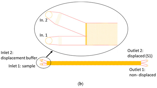
Figure 2.
Two designed and fabricated microarrays. (a) DLD design for high flow rates. Inlets 1 and 3 on the outsides are for buffer to prevent wall contact of the particle suspension and inlet 2 (middle) is for sample suspension. (b) Second DLD design for high particle concentrations and a tilt angle of α = 1°. Magnified view of the entrance region. The smaller inlet was used for sample solution at a high particle concentration.

Table 1.
Design parameters of the two DLD arrays.
Design 2 had a flatter tilt angle of α = 1° and a nearly doubled gap size of g = 40 µm to reduce the probability of clogging and agglomeration. This design had only two inlets to allow maximal throughput and was designed to displace particles above the critical diameter of 8 µm along the entire channel length.
2.1.2. Fabrication of the DLD Arrays
Since we focused on high throughput, the microfluidic systems had to be pressure-stable. Thus, silicon microtechnology was chosen as the manufacturing process for structuring the arrays from silicon with anodically bonded glass. This was identical for all array designs and was described in detail in our former publication [6]. In brief, first the arrays were structured on a 4″ silicon wafer using a standard photolithographic process and then dry etched into silicon to a height of 100 µm (design 1) and 110 µm (design 2). After a thermal oxidation step to render the system hydrophilic, the silicon wafer was anodically bonded at 700 V to a 4″ glass wafer with a thickness of 0.5 mm.
2.1.3. Experimental Setup for DLD Experiments
The DLD microsystems were fed by using a setup consisting of Cetoni Nemesys mid-pressure modules (Cetoni GmbH, Korbussen, Germany) that were equipped with Cetoni Nemesys stainless steel syringes. Syringes of different volumes were used for each measurement target as listed in Table 2. Since design 2 had only two inlets, only two modules were required for these experiments. The syringes were then connected to the microfluidic system in a pressure-tight manner. Standard high-pressure liquid chromatography (HPLC) connectors and 1/16” PEEK tubing with an inner diameter of 0.75 mm were used. The microsystem was fixed using a CNC-machined PEEK holder with sealing rings and an aluminum lid for fixation.
Table 2.
Overview of the used syringe volumes for the different experimental investigations.
The outlets and inlets of the microsystem were equipped with identical tubes (1/16” outer diameter and 0.75 mm inner diameter). These carried the different fractions under atmospheric pressure into different collection vessels. It was necessary for the tubes to be of the same length and without bends so that the flow in the microsystem was not affected by different flow resistances in the outlets.
To achieve the designated Reynolds numbers, the viscosity and density for water were used and the length was defined as the distance between posts, as is common in the DLD literature. The volumetric flow rates were adjusted to have matching flow velocity in all inlet channels, as described in more detail in our previous publication [6]. The full list of volumetric flow rates can be found in the Supplementary Material S1 Section S1, Tables S1 and S2.
For microscopic observation, a Zeiss Axio Observer inverted microscope (Zeiss, Göttingen, Germany) with a 10× objective and a 1.6× photo adapter was used. Video was recorded with a Sony Alpha 7 MKII DLSM camera (Sony, Tokyo, Japan) at 100 frames per second and a camera sensor sensitivity setting of 32,000. For evaluation, 10 s of the recorded videoframes (with each containing 10 s of only one fluorescent color) was stacked using the MAX and AVG functions within the z-project stacking tool of ImageJ 1.54 h. The resulting images were then merged within the color merge tool of ImageJ. To obtain a measurement, a line was drawn next to the array exit and, along this line, the RGB profile plot function of ImageJ was used to generate a csv table of the color intensities. These were then imported into Microsoft Excel 2021 and plotted using OriginPro 2024b. As illumination for general observation of the position and motion of bubbles, as well as finding the outlet sections, white light darkfield illumination was used. A green fluorescence filter set (470 nm exc./505 nm emm.) and a red fluorescence filter set (535 nm exc./620 nm emm.), each with corresponding single-color LEDs were used for the observation of fluorescent stained particles. In the following sections, only the differences compared to the general setup are described.
Variation of the Particle Shape and Density
The particle shape and density experiments were performed using design 1 with three inlets. To prevent the redistribution of particles in the DLD array during syringe refilling, the particle suspension was always disconnected from the system after a waiting time of 5 min. to allow for pressure compensation inside the DLD. As buffer, filtered demineralized water was used without any surfactants (filter pore size: 0.2 mm). Different binary suspensions containing fluorescent red and green particles were used as sample solutions to facilitate differentiation. The suspensions were prepared from fluorescent red melamine particles (microparticles GmbH, Berlin, Germany) and green polystyrene particles from Thermo Fisher (FluoroMax Green particles, Thermo Fisher, Schwerte, Germany), as well as elliptical elongated green polystyrene particles provided by Laura Weirauch, University of Bremen. The particle size combinations within the sample suspensions for each experiment and the corresponding Reynolds numbers are listed in Table 3.
Table 3.
Particles used in the experiments. All binary suspensions contained 0.01% (w/v) of each sort. As buffer, filtered DI-water was taken.
The size of the elliptical shaped particles was obtained by placing 1 µL suspension on a microscope slide and evaluated using a VHX-5000 3D microscope (Keyence Germany, Neu-Isenburg, Germany). The resulting short axis was 5 µm ± 1 µm and the long axis is 13 µm ± 4 µm. The larger deviation was caused by particles that are tilted inside the suspension droplet. Since the particles were only applied to our experiments, it is recommended to read the description of the particle elongation in their publication [24].
The Reynolds numbers for the density-based fractionation in Table 3, which took place in the second segment of the array, are based on the calculation of the inertial forces on the particles by Simon Reinecke, TU Berlin, and can be found in their publication [8].
Fractionation of Polydisperse Particle Suspensions
The studies were carried out using both DLD designs. In addition, three-way ball valves were used between the syringe pumps and the microsystem inlets. These allowed the syringe pumps to be refilled from a reservoir by manually closing the connection between the syringe and the microsystem, as depicted schematically in Figure 3. The illustration of the setup for design 2, containing two syringe pumps, can be found in the Supplementary Material S1 Section S2, Figure S1. This setup, with three-way ball valves, avoided the need to disconnect the access tube to refill the syringes, thus preventing sudden pressure changes. To ensure continuous dispersion of the particles in the sample, the syringe pumps were placed on a tumbling shaker plate (VWR, Radnor, PA, USA) and were additionally manually shaken every 3 min. A small number of glass beads (diameter 2.5 mm) were added into the syringe to prevent sedimentation of the sample particles. This mixing process was tested by measuring the particle size distribution of the feed suspension after 15, 30 and 40 min of pumping. Since the measurements showed no shift in size distribution, the process was considered effective and was applied to all polydisperse particle size suspensions. The syringes feeding the buffer channels were filled with pre-filtered (filter pore size of 0.2 µm) demineralized water without further surfactants. A pressure monitor (Cetoni GmbH, Korbussen, Germany) was connected between the syringe pump and the (larger) buffer inlet. The volume flow rates of the different inlets were selected to ensure a uniform inflow and are given in Table 4 with the associated Reynolds number.
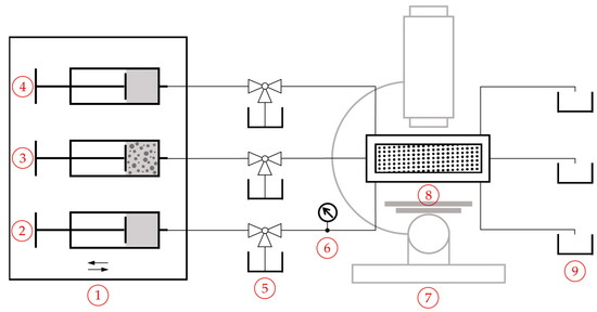
Figure 3.
Experimental setup of design 1: (1) Cetoni Nemesys pump system (Cetoni GmbH, Korbussen, Germany) with three medium pressure modules, placed on a tumbling shaker plate (VWR, Radnor, PA, USA); (2) stainless steel syringe, containing buffer 1; (3) stainless steel syringe, containing feed particle suspension; (4) stainless steel syringe, containing buffer 2; (5) Three-way ball valves to refill the syringe pumps from storage container; (6) pressure monitor; (7) Zeiss Axio Observer inverted microscope (Zeiss, Göttingen, Germany) with a 10× lens and a 1.6× photo adapter under darkfield illumination; (8) microsystem, fixed using a CNC-machined PEEK holder with sealing rings and an aluminum lid for fixation; (9) collection containers for the separated particle fraction suspensions.
Table 4.
List of the Reynolds numbers and the corresponding inlet volume flow rates.
Polydisperse silica microspheres ranging in size from 2 to 19 µm (Cospheric LLC., Somis, CA, USA) were suspended in filtered demineralized water (pore size 0.2 µm) and dispersed by vortex shaking. In order to minimize the occurrence of contamination and residual particles in the periphery, the microsystems were flushed with filtered deionized water for approx. 20 min at flow rates corresponding to a Reynolds number of Re = 30 before each test series. This procedure was previously found to be sufficient to remove the majority of the contamination. Dilutions were prepared from the original 1% (v/v) suspension. The tested particle concentrations are shown in Table 5.
Table 5.
List of the tested particle concentrations of polydisperse silica microspheres in design 1 and 2.
In contrast to the binary density- and shape-dependent separation in the previous chapters, a suspension with a continuous size distribution was used here. In order to quantify the size distributions of the separated fractions, the outlet particle fractions were collected and then analyzed using a MOXI™ Z cell counter (Orflo Technologies, Ketchum, ID, USA). The instrument combines thin-film sensor technology and the Coulter measuring principle. For the expected particle size distribution, a type S cassette (particle size: 3 µm to 20 µm) was used for the MOXI™ Z. For particle size measurement, the fractions were diluted with 1× PBS buffer (Gibco by Life Technologies Inc., Carlsbad, CA, USA). To confirm the validity of the measurement method, the feed suspension was also tested using the laser diffraction method (Mastersizer 3000, Malvern Panalytical, Almelo, The Netherlands), which gave a similar particle size distribution.
An example of the particle size number distributions is shown in Figure 4a. It consists of individual measurements of the diluted sample suspension as well as the two outlet suspensions (fine-outlet 1; coarse-outlet 2) from design 2. It should be noted that the particle measurement range of the instrument is 3–20 µm [25]. The particle number density distributions q0,x,i were calculated using Equation (5):
where Nx,i is the respective number of particles of particle size x in sample i, Ntotal,i is the total number of particles in the sample, and Δx is the selected interval width of the histogram (in this case Δx = 0.0125 µm). Gaussian functions were determined to approximate the density functions (Figure 4b). In the next step, the particle number density distributions q0,x,i were weighted by multiplying q0,x,g with the coarse material fraction g and q0,x,f with the fine material fraction f (Figure 4c). In the case of design 1 with three outlets, q0,x,m was additionally multiplied with the medium material fraction m. The coarse material fraction g, defined as the ratio of the coarse material flow to the feed material flow , was calculated according to Equation (6):
where ξg,0 and ξA,0 define the measured particle number concentration of the coarse material and of the feed sample, respectively. Df,g and Df,A denote the respective dilution factor with PBS. is the volume flow of the feed channel and is the volume flow of all buffer channels summed up. Assuming that all outlets have the same volume flow, noutlets stands for the number of outlet channels. Fine material fraction f and medium-coarse material fraction m (only for design 1) were calculated analogous to the coarse material fraction g, yielding a sum of approximately 1 (with less than 10% deviation). The partition curve T(x) is as follows:
as also depicted in Figure 4c. It indicates what proportion of the feed material fraction (as a function of the particle size) is contained in the coarse material after separation. Therefore, the steeper the degree of separation curve, the sharper the separation. The quantiles xT,25, xT,50, and xT,75 were determined from the partition curve using linear interpolation with MATLAB 2022a. The value xT,50 was defined as the separation size/Dc (median/preparative separation size). The separation efficiency κ (according to Eder) was defined as the quotient of the quantiles xT,25 and xT,75, which is a measure of the sharpness of the separation [26].

Figure 4.
Example of the particle size number distributions of the diluted samples of the feed suspension and the collected fine material (outlet 1) and coarse material (outlet 2) measured using the Coulter counter (design 2): (a) measured number of counts in samples N(x); (b) density distributions with Gaussian fit functions q0(x); (c) weighted density distributions (Gaussian fit) q0,w(x) and partition curve T(x).
2.2. Dielectrophoresis
The following section describes the design and fabrication of different channels for dielectrophoresis (DEP) as well as the combination of DLD and DEP in a microsystem. The experimental setup of the particle separation in the DEP channel is also described. In addition, the implementation of electric fields as well as electric and dielectrophoretic forces in the resolved CFD-DEM simulation code is described and validated by analytical calculations. Based on the serially combined DLD-DEP microarray, the setup of a dielectrophoresis simulation is described.
2.2.1. Designs of DEP Systems
The DEP designs in the experiments focused on cDEP, continuous dielectrophoresis, in which the electrodes create an asymmetric electric field perpendicular to the flow direction, which is then used to displace the particles within the channel. Three different electrode designs were used in the experiments, based on existing publications, as shown in Figure 5 with their main geometrical properties used here [27,28,29]. In the first design, 3D stainless steel electrodes, as depicted in Figure 5a, were placed on the sides of a straight microfluidic glass channel without contacting the fluid, since this setup was reported to generate the best electric field strength [29]. The second and third design approaches focused on the electrode at the top side of the channels to simplify the manufacturing process for the combined design. Design 2 consisted of trapezoidal electrodes, as depicted in Figure 5b. Design 3 is based on interdigitated electrodes, which are mainly used for an inhomogeneous field distribution along the channel height. This is the only design where the electric field distribution can be calculated manually [16,27]. The measurements of this design are given in Figure 5c. To test the effect of different height distances between the electrodes and the channel, in the first approach, the electrodes were placed at a distance of 200 µm to the main channel by using the top side of a glass cover. In the second approach, the electrodes were placed at a distance of roughly 20 µm to the fluid, using a PDMS cover layer between the electrodes and the fluid, as illustrated in a cross-sectional view in Figure 6.

Figure 5.
Electrode designs for dielectrophoresis: (a) design 1: inserted stainless steel electrodes; (b) design 2: trapezoidal ITO electrodes; for easier visualization, only 2 are depicted; (c) design 3: interdigitated ITO electrodes.
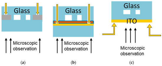
Figure 6.
Schematic cross-sectional view of the setups testing different distances between the electrodes and the fluid. The yellow arrows illustrate the electrical contact using spring-loaded contacts for the electrodes. (a) Stainless steel electrodes were inserted next to the microfluidic channel. Due to the fs-Laser manufacturing process, a minimal distance from around 200 µm could be achieved. (b) To minimize the distance between the semi-transparent ITO electrodes and the microfluidic glass channel, a thin PDMS layer (depicted in orange) was deposited as a sealing layer. Thereby, a minimal distance from around 20 µm was achieved. (c) The electrode was deposited on top of a sealing glass wafer (height: 200 µm). This process was most compatible to all other processes, since the deposition and structuring of the ITO electrode layer were the last steps in manufacturing. All combined systems were manufactured by this way; the microchannels were manufactured from silicon instead of glass.
For the design of the combined systems, structured electrodes were applied on top of the 0.2 mm sealing glass wafer. This approach is compatible with the requirement for pressure stability, whereas an additional PDMS layer will not be stable up to high Reynolds numbers. Interdigitated electrodes (Figure 5c) were placed directly on top of the DLD array to investigate the parallel fractionation, whereas above the outlet channels both designs (trapezoidal or interdigitated) were applied to investigate the serial fractionation within different systems. Contact points were placed so that both electrode structures could be controlled individually.
2.2.2. Fabrication of the DEP Systems
The first manufactured systems focused on a glass–glass system instead of silicon due to its inherent electrical properties. Thus, a 4″ glass wafer with a thickness of 0.7 mm was structured using fs-laser ablation (Microstruct-C platform from 3D-Micromag with a Pharaos light conversion Yb:KGW solid-state laser). The ablation parameters are described in another publication [30]. All structures for the channels, vias, and grooves were structured sequentially without interruption. For structuring the channels and grooves for the inserted electrodes, a repetition rate of 600 kHz was used, whereas the fluidic vias were structured using 100 kHz. For the second and third designs, only the channels and vias were structured in glass by ablation. After cleaning with water, a dip in hydrofluoric acid (HF) for 90 s followed to etch away particles and contaminants from the ablation. Another 4″ glass wafer (thickness 0.5 mm) was then thermally bonded at 650 °C for 6 h to seal the fluidic channel. The stainless steel electrodes were cut from a 100 µm thick 1.4404 stainless steel foil by fs-laser ablation and were manually inserted into the prepared cavities next to the main channel. Designs 2 and 3 were also manufactured from glass, with the exception that no grooves were required for mounting the electrodes.
The electrodes for design 2 and 3 consisted of a 100 nm sputtered ITO (Indium Tin Oxide) layer and were structured by fs-laser ablation. To test the geometric and electrical properties of the ITO layer, different patterns were transferred onto an ITO layer on a standard 4″ glass wafer to find the best filling strategies and minimal distances necessary to generate the electrodes. Contour filling with 4 equidistant lines 5 µm apart resulted in an ablated line of 40 µm width. This distance provided a sufficient electrical cut between two adjacent lines as tested with a needle connected to a standard multimeter.
For the second approach (Figure 6b), a 20 µm PDMS layer was spin coated on the structured ITO electrodes on top of a 0.7 mm glass wafer. For this, 4 mL of already mixed and degassed PDMS (ratio 10:01 PDMS:hardener) was evenly dispensed onto the electrode layer. After a dispensing step of 500 rpm for 30 s and a second step at 1000 rpm for 90 s, the PDMS layer reached a height of about 20 µm. After curing of the PDMS, the channel and the PDMS-covered electrodes were bonded together by using an oxygen plasma process.
The third approach, which was also partly used for manufacturing the combined arrays, used a 0.2 mm height cover glass wafer for thermal bonding. Since ITO is incompatible with all prior steps including the cleaning steps, the electrode layer was deposited as the last fabrication step before structuring the electrodes and dicing the systems.
The combined arrays consisted of a silicon DLD array (design 1, Section 2.1.1) that was etched to a height of 50 µm by reducing the number of cycles in the Bosch process to 53. The remaining fabrication steps were identical to the standard DLD arrays, with the exception that a glass wafer at a thickness of 0.2 mm was anodically bonded to the DLD arrays. On top of the glass cover, the ITO electrode layer was deposited and patterned by fs-laser ablation. Both DEP designs (design 2 and 3, Figure 5b,c) were applied to the combined systems. A combined system-on-a-chip mounted on a holder is shown in Figure 7.
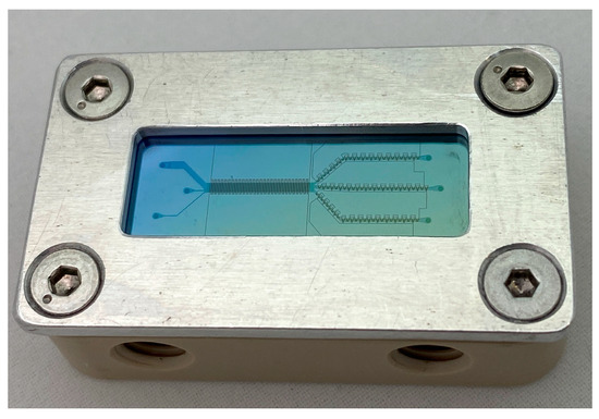
Figure 7.
Combined system mounted on an in-house manufactured PEEK holder. Parallel to the DLD array, interdigitated electrodes (design 3) are placed and along the outlet channels, trapezoidal electrodes are structured (design 2).
2.2.3. Experimental Setup
The experimental setup for DEP consisted of the two mid-pressure modules and the microscopic observation, as described in Section 2.1.3. Due to the lower flow rates of DEP, 10 mL stainless steel syringes were used for both inlets. The used sample and buffer solutions are listed in Table 6. Buffers were purchased from pH-Redox-Leitwert (Dechant GmbH, Villingen, Germany) with different conductance calibration standards at 5 µS/cm, 1 mS/cm, and 5 mS/cm. Green fluorescent PS particles of 5 µm, 8 µm, and 10 µm were used as sample solutions (5 µm and 10 µm ThermoFisher FluoroMax, distributed by Distrilab particle technology, The Netherlands, and 8 µm particles by microparticles GmbH, Berlin, Germany). Some experiments were conducted with gold-coated particles from microparticles GmbH (custom particles at 8 µm with a gold coating). In the DEP experiments, no binary suspension was used, since single particles and their interaction with the electrical field are the main focus. Therefore, only low flow rates around Re ≤ 1 were investigated to allow the particles to slowly pass through the electrode section. To electrically contact the electrodes through the holder and the glass (Figure 6a,b), the holder for the microfluidic system was modified to include a spring-loaded gold contact pin. To contact the electrodes on the top of the microsystem (Figure 6c), a 3D printed add-on was designed to hold the spring-loaded gold contact pins at the desired connection area. This was an upgrade to the existing cover of the holder, as depicted in Figure 8. This setup was used also for the combined systems and had the advantage that the existing holder could be further used. The gold contact pin was then connected to a function generator to generate voltages of 20 Vpp in the range up to 1 MHz.
Table 6.
Buffer and sample solutions for DEP experiments.

Figure 8.
Combined system with electrical contact. There is no electrical short circuit due to the aluminum holder, since the contact pads and the ITO structures are outside of the aluminum.
2.2.4. Description of the Numerical CFD-DEM Model
This chapter describes the equations on which the CFD-DEM code is based. OpenFOAM® (version 5.x), open-source computational fluid dynamics (CFD) software based on the finite volume method (FVM), was used to calculate the fields. The open source discrete element method (DEM) code LIGGGHTS (version 3.8.0) was used for the particle dynamic calculation. Both individual processes are coupled with each other using the CFDEM® (version 3.8.1) coupling software using the immersed boundary method (IBM) [31,32].
The IB-CFD-DEM code solves the velocity field and the electric field on the FVM grid. Simultaneously, the mechanical interactions between the solids (particle–particle and particle–wall), as well as the Coulomb forces in the case of particle charges and gravity, are calculated on the DEM side. During the coupling step, fluid forces are applied to the particles. Based on the calculated electric field, electric field forces (for charged particles) and dielectrophoretic forces (for an inhomogeneous electric field) are simultaneously transferred to the particles. Based on all the forces and torques acting on the particles, the particle velocities, positions, and rotations are calculated and updated. This information is fed back to the CFD to correct the field values accordingly [33].
For the continuous fluid phase, the Navier–Stokes equations for incompressible flow were solved using the PISO (Pressure-Implicit with Splitting of Operators) algorithm. In one timestep, the PISO algorithm solves the discretized equations for pressure and velocity in a linearized form, involving one predictor and two corrector steps. The Mach number lays below the critical value for compressible flows (Ma = 0.3), so the flow can be assumed incompressible. To obtain pressure and velocity fields, OpenFOAM solves the equation of continuity and the equation of the conservation of momentum. A Newtonian fluid and a constant density is assumed, which simplifies the continuity equation to:
Therefore, the momentum equation becomes the Navier–Stokes equation for an incompressible fluid:
Since we are in the inertial but still the laminar range, no turbulence model was used [34]. The electric field E, solved in the continuous field and discretized via the FVM, is obtained from the gradient of the electric potential φ:
The electrical potential φ is calculated via the Poisson equation. In the second term, in the case of free charges inside the field, q represents the charge density and εm denotes the absolute permittivity of the medium:
Furthermore, the current continuity equation is solved, based on the principle of conservation of charge:
where j is the electrical current density and k denotes the ion mobility [35]:
In the discrete phase, the differential equations (Newton–Euler) for translational and angular momentum are calculated:
Here, m is the mass of the particle, I is the second moment of area, ω is the angular velocity, and a is the center-to-surface vector. Fppw represents the particle–particle or particle–wall collision forces, Ff is the fluid drag force, and Fg describes the gravitational body force on the particle [36]. Fe denotes the electrical force und Fdep describes the dielectrophoretic force on the particle.
For an incompressible Newtonian fluid, the drag force Ff can be described as follows:
This force is developed from the product of the stress tensor of the fluid field σ and the outer normal vector of the particle , integrated over the particle surface Γs. Using the divergence theorem, this force is converted into a volume integral over the particle volume Ωs and can be split into a pressure term and a viscous term. Since the force is calculated using a discretized mesh, the following discretized form of the equation applies:
where V(c) denotes the volume of the cell c on which the force consisting of pressure and viscous components is applied. corresponds to the entirety of all cells containing solids [31].
The electric force Fe results from the product of the electric field strength E and the charge of the particle qp. For the discretized form, it must be taken into account that the electric field strength may be inhomogeneous and therefore varies in the cells. Therefore, the fraction of the force contributed by each cell is calculated and summarized for the entire particle, where α(c) corresponds to the void fraction of the cell c:
The discretized form of the dielectrophoretic force Fdep is described as follows:
Likewise, the force on the individual cells containing solid matter is calculated and summarized for the total particle.
2.2.5. Validation of the Numerical CFD-DEM Model
Simple simulation setups with known analytical solutions were used to validate the resolved force models. In these, all other force calculations such as gravity or fluid drag force were neglected to focus only on the electric force Fe and the dielectrophoretic force Fdep on a particle. In this way, it was possible to compare the movement of the particle due to the electric or dielectrophoretic force with the corresponding analytical solution.
Electrical Force on a Charged Particle
In order to calculate the electric force, a cuboid simulation domain was used with a voltage applied to opposite walls (Figure 9). Since the charge density q inside the volume is zero, the Poisson equation (Equation (11)) can be simplified to the Laplace equation and further reduced to the one-dimensional case. This results in a homogeneous electric field and thus a constant force Fe = Eqp on a charged static particle with the charge qp, which starts accelerating under its influence. Table 7 lists our selected parameters for the simulations. Figure 9c shows the particle position in the vertical axis as a function of time, both for the numerical and the analytical solution, which show a good agreement.
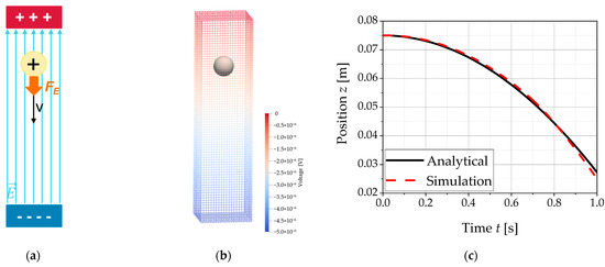
Figure 9.
The figures show the simulation setup for the validation of the force model for the electric force Fe on a charged particle in a homogeneous electric field and the result of the validation of the force models for the electrical force Fe. The values from the simulations are compared with the analytical solution: (a) schematic representation of the simulation setup; (b) discretized simulation domain with representation of the electric voltage distribution and the particle in its starting position; (c) validation of the electrical force Fe by comparing the position of a charged particle in a homogeneous electric field as a function of time.
Table 7.
List of the parameters selected for the validation of the force model for the electric force Fe.
Dielectrophoretic Force on an Uncharged Particle
An inhomogeneous electric field is the prerequisite for the dielectrophoretic force. This means that the electric field force varies depending on the location. For validation, a ring structure was simulated such as in a gas-insulated switchgear (GIS), as is shown in Figure 10. For this structure, an analytical solution exists for the electric field depending on the radial vector r [33]:
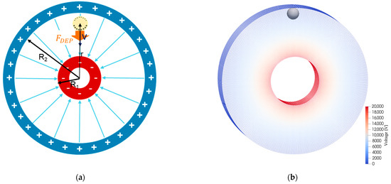
Figure 10.
The figures show the simulation setup for the validation of the force model for the dielectrophoretic force Fdep on an uncharged particle in an inhomogeneous electric field: (a) schematic representation of the simulation setup; (b) discretized simulation domain with representation of the electric voltage distribution and the particle in its starting position.
The inner annular electrode (radius R1) has the voltage Uφ applied to it, while the outer shell (radius R2) is grounded (Figure 10; selected parameters in Table 8). This creates a gradient of the electric field directed towards the inner ring, which exerts a (positive) dielectrophoretic force Fdep on the uncharged particle in the radial direction, causing the particle to move in the directing of the center of the structure:
where the inhomogeneity means the gradient of the dot product of the electric field can be described by the following equation:
Table 8.
List of the parameters selected for the validation of the force model for the dielectrophoretic force Fdep.
The electric field calculated in the FV cells as a function of the radial vector r is shown in Figure 11a and compared with the analytical solution. In addition, the integrated force exerted on the spherical particle is plotted in Figure 11b and also compared with the analytical solution, with the results also showing good agreement for this force model.
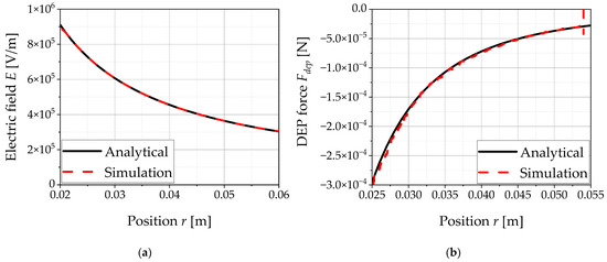
Figure 11.
The graphs show the results of the validation of the force model for the dielectrophoretic force Fdep. The values from the simulations are compared with the analytical solution: (a) electric field E as a function of the position in the ring-shaped inhomogeneous electric field; (b) dielectrophoretic force Fdep on an uncharged particle in the ring-shaped inhomogeneous electric field.
2.2.6. Model Description of the (combined) DEP Fractionation
A three-dimensional domain was used to simulate the DEP channel (Figure 12). Depicted is a section of a DEP channel with an interdigitated electrode design, in which alternately oppositely poled electrodes are connected to one side of the channel. In this approach, the laterally inserted electrodes would only be separated from the channel by a 10 µm thin, straight silicon layer, which can be neglected. Compared to the setup from Figure 6b,c, which both have larger distances between the electrodes and the fluid channel, this setup has the advantage of having the electrodes along the entire height of the channel walls and thus a lower field weakening. Due to high manufacturing challenges regarding the contacting, possible shortcut through silicon and the compatibility of the different processes, this approach has not yet been tested experimentally. This DEP channel is intended to be a part of the serially connected DLD-DEP microsystem (DLD design 1) and to be connected downstream of the DLD fractionation unit. The simulated channel section contains a pair of oppositely polarized electrodes. To reduce the computational effort, periodic boundary conditions were defined at the inlet and outlet patches in both CFD and DEM, so that the channel length was artificially multiplied by repeatedly passing the particle through the simulation domain. In addition, the depth of the segment was flattened to twice the particle diameter and the patches perpendicular to this axis were also given periodic boundary conditions.
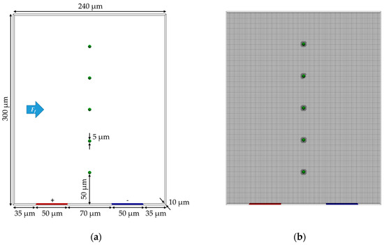
Figure 12.
Schematic representation of the simulation domain with particles. (a) Representation with dimensions and representation of the electrodes. The blue arrow indicates the flow direction. (b) Discretization and dynamic refinement of the mesh around the particles.
A momentum source was used to control the inlet velocity of the fluid to ensure that the average velocity at the inlet cross-section matched a pre-determined velocity (see Table 9 for the velocities and corresponding Re). The remaining walls delimiting the channel parallel to the flow were given no-slip Dirichlet boundary conditions for the flow velocity and Neumann boundary conditions for all other quantities. Five particles with a diameter of dp = 5 µm were placed at a uniform distance of 50 µm across the flow direction in order to investigate the influence of the electric field on different areas of the channel. Individual simulations were performed with uncoated and gold-coated PS particles. The domain was discretized using a block-structured grid and dynamically refined by a further level in the vicinity of the particles (Figure 12b). The particle is thus represented by approximately 10 cells across the diameter. The AC voltage was approximated by a steady-state simulation with a constant DC voltage equal to the root mean square voltage of the AC potential Uφ,RMS.
Table 9.
Overview of the different parameter combinations in the coupled CFD-DEM simulations.
The Clausius–Mossotti factor is calculated from the complex permittivities of the particle and the medium as follows [37]:
where the complex permittivity for a core-shell particle is defined as:
An overview of all simulation parameters can be found in Table 10. The values used result in the curve of the Clausius–Mossotti factor visible in Figure 13 for the gold-coated and uncoated PS particles as a function of the alternating current frequency. This results in the gold-coated PS particles being affected by pDEP and the uncoated PS particles by nDEP at the frequency of 1 MHz used.
Table 10.
Summary of the selected simulation parameters.
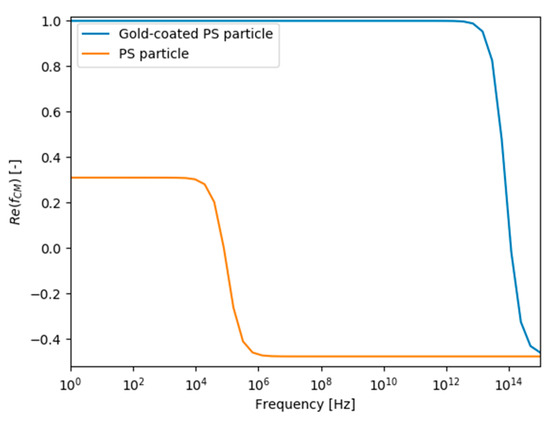
Figure 13.
Trend of the Clausius–Mossotti factor fCM as a function of the AC frequency for gold-coated and uncoated polystyrene particles with the properties shown in Table 10.
The simulations were performed on a high-performance computing cluster (CPU INTEL Xeon E5-2640v4, 25 MB cache, 2.40 GHz). The diffusion courant number () was the decisive criterion for stability [38]. It depends on the kinematic viscosity υ instead of the flow velocity, so we chose the same time step for all Reynolds numbers. As a result, the simulation time was almost inversely proportional to the Reynolds number for a given particle trajectory. A particle path of 800 µm was reached after ~40 h for Re = 10, ~75 h for Re = 5, and ~300 h for Re = 1. Due to the long simulation times, especially at the lower Reynolds numbers, it was decided not to simulate a longer distance, although the corresponding real channel was several times longer.
3. Results and Discussion
3.1. Deterministic Lateral Displacement
The following section presents the results and discussion of the separation in the DLD microsystem based on size, density, and shape as a function of Reynolds number and particle concentration.
3.1.1. Particle Density Variation
Density fractionation for 5 µm particles was shown to be possible at Re = 82. As can be seen from Figure 14, the green polystyrene (PS) particles were more displaced than the red melamine particles. To investigate the requirement of the exact Reynolds number for density fractionation, experiments at Re = 85 were carried out, with no visible fractionation. The graphs of the other measurements for 5 µm density fractionation can be found in the Supplementary Material S1 Section S2, Figure S2. Since a density dependent displacement shift is only visible at Re = 82, it is very important to precisely control the Reynolds number for the density fractionation of 5 µm particles.
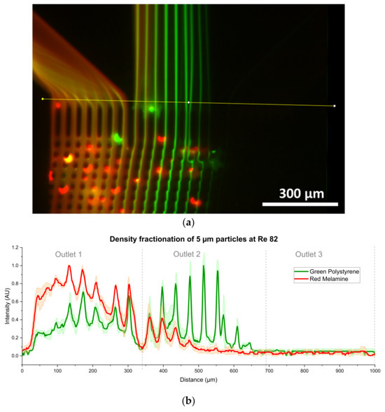
Figure 14.
Density fractionation of 5 µm particles at Re = 82: (a) the picture shows a color merge of red melamine and green polystyrene particles each consisting of a stack of 10 s video material; (b) scaled result of the red and green intensity from 3 different videos (taken on two systems) as obtained by averaging the results of the function “RGB plot” of ImageJ.
Particles at 8 µm showed no difference in motion at the calculated Reynolds number of Re = 52. However, a very small difference is visible in the experiments at Re = 50 and 55, as can be seen from Figure 15a,c. There are some additional peaks of green intensity before and after the red intensity, which could be used for a very coarse sorting of PS particles. However, these peaks are caused by a single particle following that trajectory in a single measurement, as the deviation is in the range of the intensity. The results of Figure 15 are based on two measurements on different systems. Thus, it is unlikely to achieve a good separation of 8 µm particles according to their density.

Figure 15.
Density fractionation experiments of 8 µm particles at different Reynolds numbers in binary suspensions. Overall, there is no such further displacement visible as compared to the 5 µm particles. All data are based upon two measurements on different systems. (a) Results at Re = 80. The large standard deviation indicates that the first green peaks are caused by a single particle. (b) Results at Re = 52. There is no difference between the peak position visible. (c) Results at Re = 55. As in (a), there is a large deviation that indicates an unreliable separation.
3.1.2. Variation of Particle Shape
For the first time, experimental studies were carried out with elliptical particles in the Reynolds number range of 10–80. The experiments showed, that elliptical particles have an increased chance of interacting with the posts and other particles, partially clogging the array. This leads to a fanning of the trajectory of ellipsoidal particles, which is independent of the Reynolds number. Nevertheless, in some experiments it was possible to separate elliptical from spherical particles at any Reynolds number. Figure 16a shows an image of a successful separation, with spherical and ellipsoid in one outlet and only ellipsoid in the other. The image is a composite of the red and green channels. In Figure 16b–e the measurement results for Re = 10, 40, 50 and Re = 70 are depicted. The results are based on the data evaluation of at least three videos from different microsystems. To evaluate the data for shape dependent fractionation, the MAX stacking function of ImageJ had to be sued instead of the AVG stacking function. The complete plot including all investigated Reynolds numbers can be found in the Supplementary Material S1 Section S4, Figure S3. In Figure 16b–e it can be seen that the spherical particles were not strongly affected by the ellipsoidal particles, so the displacement is comparable to that in previous publications [3,5,6]. The large error in Figure 16b is due to the fact that the green particles were only displaced this far in one of the four measurements. Unfortunately, the error in Figure 16b,d,e also indicates that the separation is not reliably repeatable. Starting from Re = 50, the green channel had a non-linear offset, particularly visible at the boundaries between the outlets, where the intensity did not reach zero. This offset was caused by brightly particles trapped near the outlet section, as can be seen in Figure 16a. Due to the existing offset, the difference in intensity caused by green particles in outlet 2 at Re = 50 (Figure 16e) is reduced in comparison to Figure 16b–d.
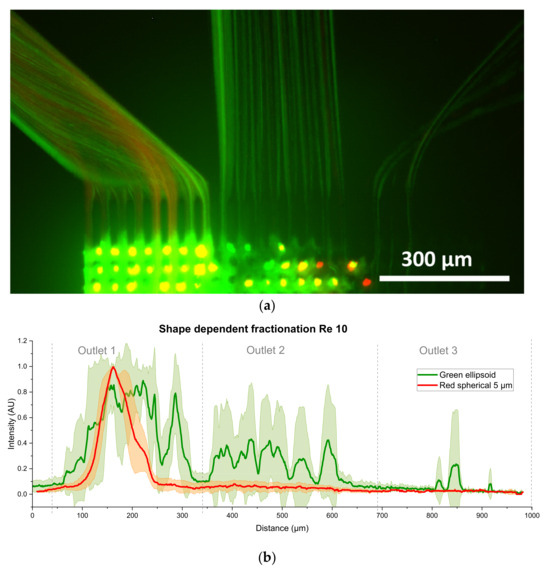

Figure 16.
Fractionation experiments of green fluorescent elliptical polystyrene and red fluorescent spherical melamine particles. (a) Image at Re = 50 containing the elliptical particles in the green channel and the spherical melamine particles in the red image channel. (b) Measurement plot for Re = 10. The error in the green channel is increased, since the further displacement of green particles was visible in 2 of 4 measurements. (c) Measurement plot for Re = 40 showing nearly identical displacement for spherical and ellipsoid particles. (d) Measurement plot for Re = 50. The increased green intensity in outlet 2 hints to a separation containing more ellipsoidal particles. (e) Measurement plot for Re = 70. Due to the large offset, caused by brightly shining particles the green signal in the second outlet is lowered.
3.1.3. Fractionation of Polydisperse Particle Suspensions
In this section, the separation behavior of the particles as a function of their size, the Reynolds number, and the particle concentration, comparatively for both microsystem designs, is presented and discussed. Figure 17 shows the weighted particle size number density distributions of the separated fractions from outlets 1 (fine) and 2 (coarse) against the feed suspension distribution and the calculated partition curves T(x) for design 2. Figure 17 shows examples of the shift in the size distributions and in the separation curves as a function of the Reynolds number and the particle concentration. In Figure 17a, the plots are stacked as a function of the increasing Reynolds number at a constant volume concentration of 0.01%. To visualize the effect of concentration, a constant Reynolds number of Re = 10 is chosen for Figure 17b, showing the effect of increasing volume concentration.
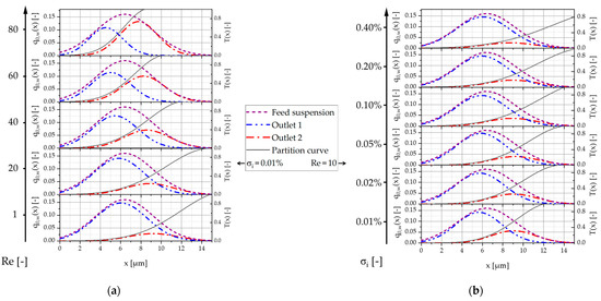
Figure 17.
Weighted particle size number density distributions of the separated fractions from outlets 1 (fine) and 2 (coarse) against the feed suspension distribution and the calculated partition curves T(x) for design 2: (a) graphs plotted stacked with increasing Reynolds number (at constant volume concentration σi = 0.01%); (b) graphs plotted stacked with increasing volume concentration (at constant Reynolds number Re = 10).
As the Reynolds number increases, the peak of the particle size distribution of outlet 2 (coarse) increases. The peak of the particle size distribution in outlet 1 (fine) decreases with increasing Reynolds number and shifts towards lower particle sizes. The partition curve shows a corresponding shift towards smaller particle sizes and is also steeper at higher Reynolds numbers. Increasing the volume concentration has the opposite effect. Here, the maximum of the particle size distribution of the measured particle fraction from outlet 2 (coarse) decreases in favor of the fraction measured in outlet 1 (fine). The separation function flattens out and only reaches a value of 0.8 (instead of 1) at the highest tested concentration of 0.4%.
The correlations between separation size and Reynolds number or volume concentration are as expected and consistent with previous research. A reduction in the critical particle diameter in the DLD microsystem with increasing Reynolds number has been repeatedly demonstrated and is due to the increase in inertia effects, changes in the flow profiles, and the formation of static vortices behind the posts [3,5,6,14,15,39,40,41,42,43].
An increase in particle concentration led to a reduction in lateral deflection and thus a decrease in the displacement mode, along with an increased particle scattering in previous studies [4,44]. This is due to the increase in particle–particle interactions, which act as a disruptive factor and reduce the determination of the deflection [4]. In addition, the larger number of particles disrupts the correct formation of streamlines and there is an increase in blockages, which can affect the flow pattern even at a distance [45]. The disruption of the displacement mode has the effect that particles above Dc increasingly tend to pass straight through the system instead of being deflected. These particles then predominantly reach outlet 1 (fine), while only a few correctly deflected particles end up in outlet 2 (coarse), as well as the misdirected particles due to the increasing scattering. This could explain why the separation function only reaches a value of 0.8 instead of 1 at the highest tested concentration of 0.4%, i.e., 20% of the largest particles end up in the fine fraction (outlet 1). However, the highest fluctuations in the measurement results also occurred at the highest concentration, so these results should be viewed with caution and further tests should be carried out.
In order to get a better overview of the influence of the parameters on the critical particle diameter and the separation efficiency, the xT,50 values of the partition curve (Figure 18) and the separation efficiencies κ (Figure 19) were plotted against Re. In addition to the measurements of the xT,50 value, here taken as critical diameter Dc, the theoretical predictions according to Equations (1) and (2) are plotted for reference. In both figures, the results for the two DLD designs are shown: Figure 18 and Figure 19 a) and b) each refer to the separation in design 1: Figure 18 and Figure 19 a) as between outlets 1 (fine) and 2 (medium-coarse) and Figure 18 and Figure 19 b) as between outlets 2 (medium-coarse) and 3 (coarse); Figure 18 and Figure 19 c) shows the results for design 2 for the separation between the only two outlets 1 (fine) and 2 (coarse). As the gap of design 2 was four times larger than the gap of design 1 and the inlet channel for the sample solution was wider (see Table 1), the blockage of the inlet region or the gap between posts is less likely. Therefore, design 2 allowed for much higher particle concentration before failure (10×), as intended.
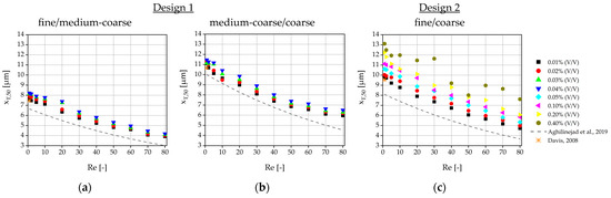
Figure 18.
Values (defined as critical particle diameter Dc) for the tested volume concentrations, plotted against the Reynolds number, compared to the analytically calculated values according to Aghilinejad et al. [3] and Davis [46]: (a) results for design 1 for the separation between outlet 1 (fine) and 2 (medium-coarse); (b) results for design 1 for the separation between outlet 2 (medium-coarse) and 3 (coarse); (c) results for design 2 for the separation between outlet 1 (fine) and 2 (coarse).
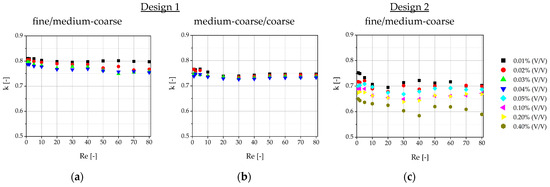
Figure 19.
Separation efficiency values κ for the tested volume concentrations, plotted against the Reynolds number: (a) results for design 1 for the separation between outlet 1 (fine) and 2 (medium-coarse); (b) results for design 1 for the separation between outlet 2 (medium-coarse) and 3 (coarse); (c) results for design 2 for the separation between outlet 1 (fine) and 2 (coarse).
The theoretical predictions as a function of the Reynolds number according to Aghilinejad et al. [3] reflect the trend well, but they underestimate the results. This is not surprising, since it has already been observed that theoretical models slightly underestimate the critical particle diameters as long as particle–particle and particle–fluid interactions are not taken into account [2,41,47]. The Davis model only considers small Reynolds numbers, but since it is empirically determined [46], it agrees well with our results for the smallest Reynolds numbers and volume concentrations. In general, the values in design 2 deviate slightly more from the theoretically predicted values than in design 1. Although design 2 had a significantly flatter deflection angle, to reduce the risk of clogging, the significantly increased channel length required is disadvantageous to fractionation as more disturbances that can occur and become more significant. This applies to unintentional lateral movement due to diffusion as well as particle–particle collisions. Also, channel irregularities or process disturbances caused by the periphery can affect the separation. This is also an explanation for the lower separation efficiency κ in design 2, compared to design 1 for the same process parameters.
As mentioned above, another factor influencing κ is the width of the sample inlet channel. As this is significantly narrower in design 1, particle guidance is more precise. The second buffer inlet channel in design 1 acts as a sheath flow and keeps the particles away from the wall. Wall effects occur in the area of the side wall, which influence the flow pattern and thus shift the critical particle diameter [41,48]. Pariset et al. [48] found that where the posts merge laterally into the walls, the streamlines are directed away from the wall, whereas they tend to be directed towards the wall in the areas where no posts intersect with the wall. There is therefore a local dependence of the critical particle that exerts an influence further away from the wall. This results in zig-zag and displacement zones for the mixed-mode particles and broadens the particle size range that moves in mixed mode. However, these wall effects are known to decrease with increasing period and width of the DLD array [48]. Design 2 is significantly wider than design 1 (almost twice as many posts in the row) and has a larger periodicity, both of which should reduce the wall effects and therefore improve the separation efficiency. However, the absence of the sheath flow could result in the wall flow having a greater influence on the particle trajectories, which in turn would promote the mixed mode and thus reduce the separation efficiency.
There are other geometric properties that promote mixed mode [6,46,48,49,50]. Anisotropic permeability is important in this context [49,50,51,52]. It occurs predominantly with the parallelogram shape of the DLD, as is the case with our microarray designs. The inclined post arrangement leads to a local tilt of the main flow in the direction of the post deflection. The pressure gradient also runs along this direction of inclination and not in the direction of the main channel. The angle between the particle deflection and the changed main flow direction is reduced, resulting in locally smaller critical particle diameters. However, as the walls restrict the main flow direction, recirculation occurs in some locations, compensating the deflection. This results in a spectrum of locally different critical particle diameters [52]. In contrast to the wall effects, the anisotropic permeability is reduced with fewer posts perpendicular to the flow. It also decreases with lower post-to-gap ratios and longer arrays [52], where design 2 should have an advantage.
The results confirm the assumption of a decrease in separation efficiency with increasing volume concentration. A decrease in separation efficiency with increasing Reynolds numbers is not observed. This was also observed simulatively in previous studies: at low particle concentrations, even an improvement in separation was observed at high Reynolds numbers compared to low Reynolds numbers [14]. When the volume fraction was increased above 3.6%, the effect was reversed [14]. In this experiment, we remain at significantly lower concentrations, so the negative effect is not expected yet. In design 1, the separation efficiency between outlets 1 (fine) and 2 (medium-coarse) is slightly higher than between outlets 2 (medium-coarse) and 3 (coarse). The reason for this could be that the displacement mode is more unstable and more prone to failures, and thus more likely falls into mixed mode than the zig-zag mode.
Based on our results, we have a few suggestions on how to improve the separation performance and separation efficiency: design 2 had a wider particle inlet and a large gap-to-Dc ratio compared to design 1. This allowed for an increased particle concentration at the expense of a lower separation efficiency of design 2. Therefore, a suitable or sufficient intermediate path must be found for the individual application. It would also be possible to pass the suspension through the microarray multiple times. In order to reduce wall effects, it is advisable to design wider microsystems and, if possible, to use a sheath flow buffer channel. However, the sample inlet should still be wide enough to prevent excessive dilution through the buffer channels and clogging of the inlet channel. Another option is to reduce the wall effects and promote a uniform flow pattern by specifically designing the post gap at the wall boundaries [53]. The effect of anisotropic permeability occurs only with the rhombic DLD shape and not with the rotated square shape. For binary DLD microsystems in particular, there is no reason why the rotated square shape should not be used instead, in order to avoid the effect of anisotropic permeability.
As there are large fluctuations, particularly at the higher particle concentrations in particular, further tests should be carried out to obtain an overview of mean values and standard deviations. It would also be advisable to adapt the microsystems as suggested in order to reduce the mixed mode and thus increase the separation efficiency and, if necessary, to test other DLD geometries for their suitability for high throughputs.
3.2. Dielectrophoresis
In the following, the simulative and experimental results of dielectrophoresis in the combined DLD-DEP microarray are presented and analyzed.
3.2.1. Simulations
In the following, the electric field and the field forces of the simulation domain described in Figure 12 and Figure 20a are presented below. In addition, the trajectory of the particles introduced into the channel is described and discussed. Figure 20b shows the electric field calculated in the simulation domain using the FVM as a function of the position resulting from the voltage applied to the planar electrode pair on one of the lateral walls of the simulated channel section. The electric field has its maxima at the edges of the electrodes and decreases towards the center of the electrodes or the gaps. At greater distances from the wall equipped with the electrodes, the electric field becomes largely independent of the horizontal axis. In the direction of the opposite wall, the decrease in the electric field is exponential. The area near the opposite wall again shows a variation of the electric field as a function of the horizontal axis, with the electric field being minimal towards the center of the electrodes and increasing towards the center of the gap. This resembles the pattern described by Crews et al. [54]. The aforementioned authors have also developed a mathematical equation for the gradient of the square of the electric field that describes the center area between the wall occupied by the electrodes and the opposite wall (gradient term), which is independent of the horizontal axis. The described exponential function depends on the electrode width and the electrode gap width, as well as the root mean square voltage Uφ,RMS [54]. This allowed us to compare the analytically determined solution of this region with the results of our simulations (Figure 20c). Here the gradient of the square of the electric field is shown for our simulations, in the line above the electrode gap center, at the electrode edge, and at the electrode center. While these show a variation near the walls, they are all in line in the central region. This line is consistent with the model of Crews et al. [54], so we can confirm it with our results. Sadeghian et al. [55] confirm the largest gradient in the region of the electrode edges and the relatively smallest gradient between the electrodes in the gap. pDEP acts in the direction of the electrodes, while nDEP acts away from the electrodes, meaning that the particles experiencing nDEP are being flushed away by the fluid. The force acting on the particles depends on the distance between the electrodes, their gap, and the ratio of the width to the gap, as well as on the channel dimensions [55].
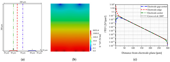
Figure 20.
Results of the calculation of the inhomogeneous E-field of an interdigitated electrode DEP microarray section using the FVM: (a) schematic of the simulation domain, showing the location of the lateral electrode pair; (b) the color diagram shows the distribution of the electric field in the simulation domain; (c) electric field gradient square at three different perpendicular lines to the channel (depicted in (a)) and comparison with the model for the gradient term according to Crews et al. [54].
For successful separation, the target particles should be deflected sufficiently over the existing channel length to allow spatial segregation. The deflection is directly depending on the dielectrophoretic force (Equation (3)). To maximize the force, the electric field gradient should be maximized. The most important parameters are the electrode width and gap, the channel width, and the choice of the magnitude of the applied AC voltage. In addition, the channel length must be sufficient for the selected volume flow rate. Increasing the fluid velocity requires a stronger electric field in order to achieve a sufficiently large DEP force and to move particles efficiently [56]. It should also be noted that the electric field, and thus the DEP forces, decreases very rapidly with the axis directed away from the electrodes [56]. The starting position of the particles can therefore be decisive for the separation. Since in our case the material-dependent particle separation via DEP is to take place on a shared microchip following the size-dependent separation via DLD (multi-dimensional separation), we are subject to a number of restrictions: 1. The volume flow corresponds to that of the previous particle separation via DLD. The separate control of the flow velocity in the DEP channel can only be achieved by means of the choice of the channel cross-section. 2. The position of the particles at the inlet is arbitrary and can be located either close to the electrodes or close to the opposite wall. 3. Different particle size ranges are to be expected in the channels downstream of the DLD size separation, the limits of which can be shifted depending on the volume flow rate used (Reynolds number). In the following analyses, we describe the DEP results in relation to the Reynolds numbers present in the DLD section at the given volume flows. Due to the different dimensions and calculation method using the hydraulic diameter as the critical length, the Reynolds number in the DEP channels differs with respect to the DLD array. All the parameters used are shown in Figure 12 and Table 9 and Table 10. It should be noted that the depth of the channel in the DEP section corresponds to the DLD section and the entire channel has about 30 electrode pairs, as simulated in a single section using periodic boundary conditions. With a size of 5 µm, the simulated test particles are below the first DLD separation size for small Re and in the range of the separation size for large Re. Improved deflection is to be expected for larger particles, as FDEP increases with the particle volume. The Clausius–Mossotti factor, although size-dependent, remains unchanged in our particle size range under otherwise constant conditions.
Figure 21 shows the particle trajectories over the length of the passed DEP channel for three different Reynolds numbers (based on the DLD section). As can be seen in Figure 21, most of the particles that were introduced in the section of the channel near the electrode level are deflected. Here, the gold-coated PS particles (solid lines) were deflected in the direction of the electrode plane (pDEP). In contrast, the uncoated PS particles (dashed lines) were slightly deflected in the opposite direction (nDEP). This occurs earliest at the lowest Reynolds number tested, Re = 1, for the two particles initiated furthest from the electrode wall. At a Reynolds number of 5 and 10, the gold-coated PS particle nearest to the electrodes is also completely deflected. As expected, the distance travelled in the main flow direction increases with the Reynolds number until complete separation occurs. The particle second closest to the electrode wall is expected to be fully deflected along the entire length of the channel at a Reynolds number of Re = 5; at Re = 10 the channel length is probably not sufficient. The trajectories of the uncoated PS particles experiencing nDEP approach a line that is not expected to extend beyond the center of the channel.
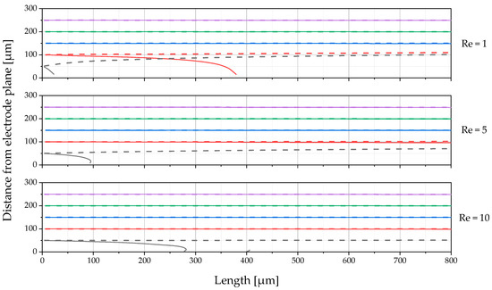
Figure 21.
Simulated trajectory of the five particles initiated at different channel positions (differentiated by color), calculated for three different Reynolds numbers applying to the upstream DLD array. The solid lines indicate the trajectories of the gold-coated PS particles (pDEP), and the dashed lines of the same color represent the trajectories of the uncoated PS particles (nDEP) initiated at the same position.
The results show that fractionation is successful when limited to lower volume flows. Partial separation or concentration must be assumed here, as particles that are too far away from the electrodes are not subjected to sufficient forces. Therefore, it is likely that separation would be significantly improved if the particles were initially concentrated in the half of the channel next to the electrodes. Due to the upstream DLD part in the microarray, it would be very complex to use a sheath flow for this, as it would have to be matched to the pressure in the respective channels. A promising option for this purpose would therefore be sheathless particle-focusing methods. For example, it would be possible to place a second DLD section upstream of the DEP section, which is dimensioned to direct all particles towards the electrode wall. Active methods would also be an option, for example, acoustic focusing [57]. The focusing methods would have to be individually dimensioned and adapted for the respective outlet channels of the DLD section, as the particle sizes will be different in each channel.
It should be considered that the particles experiencing pDEP are significantly more affected than those experiencing nDEP. Therefore, it may be difficult to feed both types of particles into different outlet channels at the same time. Sadeghian et al. [55] use a two-stage process, where the particles that are subjected to pDEP forces are first collected on a wall using voltage. Meanwhile, the nDEP particles are washed out and collected. The voltage is then switched off and only buffers are introduced into the system. The collected pDEP particles are now washed out and collected separately [55]. Such a procedure is also recommended in our combined DLD-DEP microsystem, as the particles experiencing pDEP forces are likely to be slowed down considerably by the stronger forces and may even adhere to the electrodes. This can lead to chain-like agglomerations (pearl-chain effect) and thus to bridging (short circuits) between the electrodes. In addition, large agglomerates narrow the channel, which can change the flow rate and possibly also lead to blockage of the channel [56]. Two-stage separation processes are not uncommon in industry. In chromatography, for example, proteins are often adsorbed onto the solid phase and then eluted in a second step with a different buffer [58]. A multi-stage process can also be found in the magnetic fishing of paramagnetic nanoparticles [59].
In order to increase the efficiency of the separation and to enable higher flow rates, the arrangement of the electrodes could possibly be further improved. Using FEM simulations, Sadeghian et al. found that the interdigitated electrode DEP design is most efficient when the channel height is similar to the electrode pitch (electrode center-to-center distance), i.e., when the pitch/height ratio is approximately 1 [55]. In our tested system, the ratio is 0.4. According to Sadeghian et al., at this value, the capture time (i.e., the time it takes for pDEP particles to be completely deflected) is a multiple of the capture time at a ratio of 1, especially for particles whose starting position is further away from the electrodes. The channel height should be as low as possible (taking into account the increased fluid velocity for the same volume flow) and the ratio of electrode width to electrode pitch should be as large as possible, but at least greater than 0.5. Our system is slightly below this, with 0.417. In addition to the external dimensions of the electrodes, changing the shape of the electrodes may also improve the separation efficiency. For example, Wang et al. have found that the use of cylindrical electrodes instead of planar ones resulted in a more evenly distributed and overall higher electric field gradient squared [56]. However, the increased manufacturing complexity must also be taken into account.
The higher the applied (AC) voltage, the higher the DEP force on the particles and the better the expected deflection [55]. However, it should be mentioned that high voltages also lead to resistive heating [60]. Inorganic particles are less likely to be damaged by heating than, for example, biological cells such as blood particles. However, the Joule heating induced by the electric field in the inhomogeneous electric field leads to a non-uniform temperature distribution, which causes changes in conductivity and permittivity, and thus a time-averaged volume force that leads to electrothermal flow. This electrothermal flow can impose a Stokes drag force on the particles, which acts away from the electrode plane at the electrode centers and towards the electrode plane at the electrode gaps [60]. Excessive heating and the resulting induced effects can be counteracted by increasing the volume flow. As the separation efficiency is reduced by increasing the volume flow, a reasonable balance between the two parameters must be found.
These investigations are a first attempt to combine the DLD and DEP principles on a single chip in such a way that (in serial configuration) particles can be separated according to multiple separation characteristics. On this basis, the arrangement and shape of the electrodes and the channel can be optimized to achieve efficient separation at the lowest possible applied voltage.
3.2.2. Experimental Results Dielectrophoresis and Combined Systems
As described in the simulation section, a voltage of Uφ,pp = 20 Vpp was not sufficient to generate a sufficient dielectrophoretic force for efficient particle fractionation. Even with only a small PDMS layer between the buffer and the electrodes, no effect on the particles was observed. Due to the project requirements of being adjustable to different material properties, and to allow for high throughput, DC voltages could not be used. However, high DC voltages also lead to parasitic effects such as electrophoresis and Joule heating that interfere with the functionality of the DEP mechanism, as described in the section above.
The contact between the spring-loaded contact pins and the ITO electrodes was tested with needles contacting the electrode and, on the other side, the standard electrical connection of the pins to a multimeter measuring the resistance. Therefore, we suggest using an HF amplifier capable of delivering up to 1 MHz and 150 Vpp. To test the frequency required for particle manipulation, 2 µL of sample solution was applied to the ITO electrodes on the cover glass. As soon as the voltage of 30 kHz was applied to the electrodes, a movement of the PS particles in the 1 mS/cm buffer was visible. However, there was no detectable effect of the electrical field on slowly moving particles.
4. Conclusions
In this work, several studies were carried out on the separation of particles based on a variety of particle properties. Two microfluidic separation principles were investigated, namely, deterministic lateral displacement and dielectrophoresis, which were also combined on one chip for multi-dimensional separation. A particular focus of the investigations was to increase throughput, so the influence of increased Reynolds numbers, but also higher particle concentrations, was analyzed. The aim was to investigate a use beyond analytical applications to the industrial production of particle suspensions with defined properties. In the following, we would like to summarize the findings of our investigations:
- In the DLD, a density-dependent fractionation was experimentally visible for melamine and polystyrene particles of 5 µm at Re = 82, which appeared to be very sensitive to this certain flow conditions.
- Elliptical particles of size 5 × 10 µm could be experimentally separated from spherical melamine particles in the DLD.
- Polydisperse silica particles were separated in two different DLD designs under the influence of different Reynolds numbers and particle concentrations.
- In general, the separation size decreased with increasing Reynolds number, but increased with increasing particle concentration due to the intensifying particle interactions. The separation efficiency decreased with increasing particle concentration, but showed no clear dependence on the Reynolds number.
- Design 1 (three inlets including sheath flow) showed higher separation efficiencies, but allowed lower concentrations than design 2 (two inlets; significantly wider particle inlet; flatter tilt angle with significantly enlarged gap).
- The IB-CFD-DEM software has been extended to include the calculation of electric fields in the FV cells and, based on this, the calculation of electric and dielectric forces on spherical particles. The implemented force models were validated by comparing simple test cases with the analytical solutions.
- The DEP section of the serial-combined DLD-DEP design was simulated using this software at different Reynolds numbers for the separation of 5 µm polystyrene particles from gold-coated polystyrene particles. A good deflection of the core-shell particles was observed in the half of the channel near the electrodes, which decreased with increasing Reynolds number. The half of the channel averted from the electrodes showed negligible deflection, which is why the inclusion of an additional particle-focusing section between the DLD and DEP sections is recommended to concentrate the particles to the electrodes.
Supplementary Materials
The following supporting information can be downloaded at: https://www.mdpi.com/article/10.3390/powders4020013/s1, Supplementary Material S1 containing sections S1–S4. Table S1: List of flow rates used for density fractionation. Table S2: List of flow rates used for shape dependent fractionation. Figure S1: Experimental setup of design 2: (1) Cetoni Nemesys pump system (Cetoni GmbH, Korbussen Germany) with two medium pressure modules, placed on a tumbling shaker plate (VWR, Radnor, PA, USA); (2) stainless steel syringe, containing feed particle suspension; (3) stainless steel syringe, containing buffer; (4) three-way ball valves to refill the syringe pumps from storage container; (5) pressure monitor; (6) Zeiss Axio Observer inverted microscope (Zeiss, Göttingen, Germany) with a 10x lens and a 1.6x photo adapter under darkfield illumination; (7) microsystem, fixed using a CNC-machined PEEK holder with sealing rings and an aluminum lid for fixation; (8) collection containers for the separated particle fraction suspensions; Figure S2: Density-dependent fractionation of 5 µm particles made from polystyrene and melamine. At this condition, no further displacement of any particle is visible; Figure S3: Overview of all measurements of shape-dependent fractionation. Due to the “MAX” stacking algorithm, an offset was induced in the green channel. For Re = 60, only one dataset was taken, therefore on this graph there are no error bars.
Author Contributions
Methodology, J.K. and M.S.W.; software, J.K. and M.S.W.; validation, J.K., M.S.W. and Z.L.; formal analysis, J.K., M.S.W. and Z.L.; investigation, J.K., M.S.W. and Z.L.; resources, A.K. and A.D.; data curation, J.K., M.S.W. and Z.L.; writing—original draft preparation, J.K. and M.S.W.; writing—review and editing, I.K., A.K and A.D.; visualization, J.K. and M.S.W.; supervision, I.K., A.K. and A.D.; project administration, A.K. and A.D.; funding acquisition, A.K. and A.D. All authors have read and agreed to the published version of the manuscript.
Funding
This research was funded by the German Research Foundation (DFG) within the priority program “MehrDimPart” (SPP2045), grant numbers KW 9/29-2 and DI 1934/9-2.
Data Availability Statement
The data that support the findings of this study are available on reasonable request.
Acknowledgments
The authors would like to thank Simon Reinecke for providing us with the Reynolds numbers for density fractionation in our specific design. Furthermore, we would like to thank Laura Weirauch and Jasper Giesler for providing us with elongated particles, as well as some gold-coated particles, and their cooperation in relation to dielectrophoresis.
Conflicts of Interest
The authors declare no conflicts of interest.
References
- Shekunov, B.Y.; Chattopadhyay, P.; Tong, H.H.Y.; Chow, A.H.L. Particle size analysis in pharmaceutics: Principles, methods and applications. Pharm. Res. 2007, 24, 203–227. [Google Scholar] [CrossRef] [PubMed]
- Salafi, T.; Zhang, Y.; Zhang, Y. A Review on Deterministic Lateral Displacement for Particle Separation and Detection. Nano-Micro Lett. 2019, 11, 77. [Google Scholar] [CrossRef] [PubMed]
- Aghilinejad, A.; Aghaamoo, M.; Chen, X. On the transport of particles/cells in high-throughput deterministic lateral displacement devices: Implications for circulating tumor cell separation. Biomicrofluidics 2019, 13, 34112. [Google Scholar] [CrossRef] [PubMed]
- Vernekar, R.; Krüger, T. Breakdown of deterministic lateral displacement efficiency for non-dilute suspensions: A numerical study. Med. Eng. Phys. 2015, 37, 845–854. [Google Scholar] [CrossRef]
- Dincau, B.M.; Aghilinejad, A.; Hammersley, T.; Chen, X.; Kim, J.-H. Deterministic lateral displacement (DLD) in the high Reynolds number regime: High-throughput and dynamic separation characteristics. Microfluid. Nanofluid. 2018, 22, 59. [Google Scholar] [CrossRef]
- Kottmeier, J.; Wullenweber, M.S.; Kampen, I.; Kwade, A.; Dietzel, A. A High-Aspect-Ratio Deterministic Lateral Displacement Array for High-Throughput Fractionation. Micromachines 2024, 15, 802. [Google Scholar] [CrossRef]
- Mallorie, C.; Vernekar, R.; Owen, B.; Inglis, D.W.; Krüger, T. Numerical analysis of flow anisotropy in rotated-square deterministic lateral displacement devices at moderate Reynolds number. Phys. Rev. Fluids 2024, 9, 024203. [Google Scholar] [CrossRef]
- Reinecke, S.R.; Blahout, S.; Rosemann, T.; Kravets, B.; Wullenweber, M.; Kwade, A.; Hussong, J.; Kruggel-Emden, H. DEM-LBM simulation of multidimensional fractionation by size and density through deterministic lateral displacement at various Reynolds numbers. Powder Technol. 2021, 385, 418–433. [Google Scholar] [CrossRef]
- Bowman, T.J.; Drazer, G.; Frechette, J. Inertia and scaling in deterministic lateral displacement. Biomicrofluidics 2013, 7, 64111. [Google Scholar] [CrossRef]
- Holm, S.H.; Beech, J.P.; Tegenfeldt, J.O. Combined density and size-based sorting in deterministic lateral displacement devices. In Proceedings of the 17th International Conference on Miniaturized Systems for Chemistry and Life Sciences (MicroTAS 2013), Freiburg, Germany, 27–31 October 2013; Zengerle, R., Ed.; Curran: Red Hook, NY, USA, 2014; pp. 1224–1226, ISBN 9781632666246. [Google Scholar]
- Holm, S.H.; Beech, J.P.; Barrett, M.P.; Tegenfeldt, J.O. Simplifying microfluidic separation devices towards field-detection of blood parasites. Anal. Methods 2016, 8, 3291–3300. [Google Scholar] [CrossRef]
- Beech, J.P.; Ho, B.D.; Garriss, G.; Oliveira, V.; Henriques-Normark, B.; Tegenfeldt, J.O. Separation of pathogenic bacteria by chain length. Anal. Chim. Acta 2018, 1000, 223–231. [Google Scholar] [CrossRef] [PubMed]
- Di Carlo, D. Inertial microfluidics. Lab. Chip 2009, 9, 3038–3046. [Google Scholar] [CrossRef] [PubMed]
- Wullenweber, M.S.; Kottmeier, J.; Kampen, I.; Dietzel, A.; Kwade, A. Numerical Study on High Throughput and High Solid Particle Separation in Deterministic Lateral Displacement Microarrays. Processes 2023, 11, 2438. [Google Scholar] [CrossRef]
- Lubbersen, Y.S.; Schutyser, M.; Boom, R.M. Suspension separation with deterministic ratchets at moderate Reynolds numbers. Chem. Eng. Sci. 2012, 73, 314–320. [Google Scholar] [CrossRef]
- Pethig, R. Dielectrophoresis: Theory, Methodology and Biological Applications, 1st ed.; Wiley: Hoboken, NJ, USA; Chichester, UK, 2017; ISBN 9781118671450. [Google Scholar]
- Giesler, J.; Weirauch, L.; Thöming, J.; Baune, M.; Pesch, G.R. Separating microparticles by material and size using dielectrophoretic chromatography with frequency modulation. Sci. Rep. 2021, 11, 16861. [Google Scholar] [CrossRef]
- Douglas, T.A.; Alinezhadbalalami, N.; Balani, N.; Schmelz, E.M.; Davalos, R.V. Separation of Macrophages and Fibroblasts Using Contactless Dielectrophoresis and a Novel ImageJ Macro. Bioelectricity 2019, 1, 49–55. [Google Scholar] [CrossRef]
- Al-Ali, A.; Waheed, W.; Abu-Nada, E.; Alazzam, A. A review of active and passive hybrid systems based on Dielectrophoresis for the manipulation of microparticles. J. Chromatogr. A 2022, 1676, 463268. [Google Scholar] [CrossRef]
- Yan, S.; Zhang, J.; Yuan, D.; Li, W. Hybrid microfluidics combined with active and passive approaches for continuous cell separation. Electrophoresis 2017, 38, 238–249. [Google Scholar] [CrossRef]
- Cha, H.; Fallahi, H.; Dai, Y.; Yuan, D.; An, H.; Nguyen, N.-T.; Zhang, J. Multiphysics microfluidics for cell manipulation and separation: A review. Lab. Chip 2022, 22, 423–444. [Google Scholar] [CrossRef]
- Peng, T.; Zhang, Z.; Yuan, S.; Qiang, J.; Jia, Y. Investigation on sheathless inertial focusing within low-aspect ratio spiral microchannel for cascaded microfluidic tumor cell separation. Phys. Fluids 2024, 36, 077153. [Google Scholar] [CrossRef]
- Zhou, Y.; Ma, Z.; Ai, Y. Hybrid microfluidic sorting of rare cells based on high throughput inertial focusing and high accuracy acoustic manipulation. RSC Adv. 2019, 9, 31186–31195. [Google Scholar] [CrossRef] [PubMed]
- Weirauch, L.; Giesler, J.; Pesch, G.R.; Baune, M.; Thöming, J. Sorting microparticle mixtures by multiple properties in a single dielectrophoretic filter. Results Eng. 2024, 23, 102641. [Google Scholar] [CrossRef]
- Dittami, G.M.; Sethi, M.; Rabbitt, R.D.; Ayliffe, H.E. Determination of mammalian cell counts, cell size and cell health using the Moxi Z mini automated cell counter. J. Vis. Exp. 2012, 64, 3842. [Google Scholar] [CrossRef]
- Stieß, M. Mechanische Verfahrenstechnik—Partikeltechnologie 1; Springer: Berlin/Heidelberg, Germany, 2009; ISBN 978-3-540-32551-2. [Google Scholar]
- Li, H. Dielectrophoretic separation and manipulation of live and heat-treated cells of Listeria on microfabricated devices with interdigitated electrodes. Sens. Actuators B Chem. 2002, 86, 215–221. [Google Scholar] [CrossRef]
- Choi, S.; Park, J.-K. Microfluidic system for dielectrophoretic separation based on a trapezoidal electrode array. Lab. Chip 2005, 5, 1161–1167. [Google Scholar] [CrossRef]
- Wang, Y.; Wang, J.; Wu, X.; Jiang, Z.; Wang, W. Dielectrophoretic separation of microalgae cells in ballast water in a microfluidic chip. Electrophoresis 2019, 40, 969–978. [Google Scholar] [CrossRef]
- Al-Halhouli, A.; Albagdady, A.; Al-Faqheri, W.; Kottmeier, J.; Meinen, S.; Frey, L.J.; Krull, R.; Dietzel, A. Enhanced inertial focusing of microparticles and cells by integrating trapezoidal microchambers in spiral microfluidic channels. RSC Adv. 2019, 9, 19197–19204. [Google Scholar] [CrossRef]
- Hager, A.; Kloss, C.; Pirker, S.; Goniva, C. Parallel Resolved Open Source CFD-DEM: Method, Validation and Application. J. Comput. Multiph. Flows 2014, 6, 13–27. [Google Scholar] [CrossRef]
- Goniva, C.; Kloss, C.; Deen, N.G.; Kuipers, J.A.; Pirker, S. Influence of rolling friction on single spout fluidized bed simulation. Particuology 2012, 10, 582–591. [Google Scholar] [CrossRef]
- Wang, Z.; Liu, M.; Yang, X. A four-way coupled CFD-DEM modeling framework for charged particles under electrical field with applications to gas insulated switchgears. Powder Technol. 2020, 373, 433–445. [Google Scholar] [CrossRef]
- Ferziger, J.H.; Perić, M. Numerische Strömungsmechanik; Springer: Berlin/Heidelberg, Germany, 2008; ISBN 978-3-540-68228-8. [Google Scholar]
- Moayedi, H.; Amanifard, N.; Deylami, H.M. Evaluation of using micropolar fluid approach for the EHD-enhanced forced convection through a rectangular channel using multiple electrode arrangements. Appl. Therm. Eng. 2019, 159, 113857. [Google Scholar] [CrossRef]
- Aycock, K.I.; Campbell, R.L.; Manning, K.B.; Craven, B.A. A resolved two-way coupled CFD/6-DOF approach for predicting embolus transport and the embolus-trapping efficiency of IVC filters. Biomech. Model. Mechanobiol. 2017, 16, 851–869. [Google Scholar] [CrossRef] [PubMed]
- Cetin, B.; Li, D. Dielectrophoresis in microfluidics technology. Electrophoresis 2011, 32, 2410–2427. [Google Scholar] [CrossRef] [PubMed]
- Zielina, M.; Bielski, A.; Młyńska, A. Leaching of chromium and lead from the cement mortar lining into the flowing drinking water shortly after pipeline rehabilitation. J. Clean. Prod. 2022, 362, 132512. [Google Scholar] [CrossRef]
- Lubbersen, Y.S.; Dijkshoorn, J.P.; Schutyser, M.; Boom, R.M. Visualization of inertial flow in deterministic ratchets. Sep. Purif. Technol. 2013, 109, 33–39. [Google Scholar] [CrossRef]
- Lubbersen, Y.S.; Boom, R.M.; Schutyser, M. High throughput particle separation with a mirrored deterministic ratchet design. Chem. Eng. Process. Process Intensif. 2014, 77, 42–49. [Google Scholar] [CrossRef]
- Wullenweber, M.S.; Kottmeier, J.; Kampen, I.; Dietzel, A.; Kwade, A. Simulative Investigation of Different DLD Microsystem Designs with Increased Reynolds Numbers Using a Two-Way Coupled IBM-CFD/6-DOF Approach. Processes 2022, 10, 403. [Google Scholar] [CrossRef]
- Kottmeier, J.; Wullenweber, M.; Blahout, S.; Hussong, J.; Kampen, I.; Kwade, A.; Dietzel, A. Accelerated Particle Separation in a DLD Device at Re 1 Investigated by Means of µPIV. Micromachines 2019, 10, 768. [Google Scholar] [CrossRef]
- Dincau, B.M.; Aghilinejad, A.; Chen, X.; Moon, S.Y.; Kim, J.-H. Vortex-free high-Reynolds deterministic lateral displacement (DLD) via airfoil pillars. Microfluid. Nanofluid. 2018, 22, 137. [Google Scholar] [CrossRef]
- Holm, S.H.; Zhang, Z.; Beech, J.P.; Gompper, G.; Fedosov, D.A.; Tegenfeldt, J.O. Microfluidic Particle Sorting in Concentrated Erythrocyte Suspensions. Phys. Rev. Appl. 2019, 12, 014051. [Google Scholar] [CrossRef]
- Beech, J. Microfluidics Separation and Analysis of Biological Particles; Lund University: Lund, Sweden, 2011. [Google Scholar]
- Hochstetter, A.; Vernekar, R.; Austin, R.H.; Becker, H.; Beech, J.P.; Fedosov, D.A.; Gompper, G.; Kim, S.-C.; Smith, J.T.; Stolovitzky, G.; et al. Deterministic Lateral Displacement: Challenges and Perspectives. ACS Nano 2020, 14, 10784–10795. [Google Scholar] [CrossRef] [PubMed]
- Davis, J.A. Microfluidic Separation of Blood Components through Deterministic Lateral Displacement. Ph.D. Thesis, Princeton University, Princeton, NJ, USA, 2008. [Google Scholar]
- Pariset, E.; Pudda, C.; Boizot, F.; Verplanck, N.; Berthier, J.; Thuaire, A.; Agache, V. Anticipating Cutoff Diameters in Deterministic Lateral Displacement (DLD) Microfluidic Devices for an Optimized Particle Separation. Small 2017, 13, 1701901. [Google Scholar] [CrossRef] [PubMed]
- Kulrattanarak, T.; van der Sman, R.G.M.; Schroën, C.G.P.H.; Boom, R.M. Analysis of mixed motion in deterministic ratchets via experiment and particle simulation. Microfluid. Nanofluid. 2011, 10, 843–853. [Google Scholar] [CrossRef]
- Kulrattanarak, T.; van der Sman, R.G.M.; Lubbersen, Y.S.; Schroën, C.G.P.H.; Pham, H.T.M.; Sarro, P.M.; Boom, R.M. Mixed motion in deterministic ratchets due to anisotropic permeability. J. Colloid. Interface Sci. 2011, 354, 7–14. [Google Scholar] [CrossRef]
- Kim, S.-C.; Wunsch, B.H.; Hu, H.; Smith, J.T.; Austin, R.H.; Stolovitzky, G. Broken flow symmetry explains the dynamics of small particles in deterministic lateral displacement arrays. Proc. Natl. Acad. Sci. USA 2017, 114, E5034–E5041. [Google Scholar] [CrossRef]
- Vernekar, R.; Krüger, T.; Loutherback, K.; Morton, K.; Inglis, D.W. Anisotropic permeability in deterministic lateral displacement arrays. Lab. Chip 2017, 17, 3318–3330. [Google Scholar] [CrossRef]
- Inglis, D.W. Efficient microfluidic particle separation arrays. Appl. Phys. Lett. 2009, 94, 13510. [Google Scholar] [CrossRef]
- Crews, N.; Darabi, J.; Voglewede, P.; Guo, F.; Bayoumi, A. An analysis of interdigitated electrode geometry for dielectrophoretic particle transport in micro-fluidics. Sens. Actuators B Chem. 2007, 125, 672–679. [Google Scholar] [CrossRef]
- Sadeghian, H.; Hojjat, Y.; Soleimani, M. Interdigitated electrode design and optimization for dielectrophoresis cell separation actuators. J. Electrost. 2017, 86, 41–49. [Google Scholar] [CrossRef]
- Wang, Y.; Du, F.; Baune, M.; Thöming, J. Dielectrophoresis in aqueous suspension: Impact of electrode configuration. Microfluid. Nanofluid. 2014, 17, 499–507. [Google Scholar] [CrossRef]
- Xuan, X.; Zhu, J.; Church, C. Particle focusing in microfluidic devices. Microfluid. Nanofluid. 2010, 9, 1–16. [Google Scholar] [CrossRef]
- Adamíková, J.; Antošová, M.; Polakovič, M. Chromatographic purification of recombinant human erythropoietin. Biotechnol. Lett. 2019, 41, 483–493. [Google Scholar] [CrossRef] [PubMed]
- de Lima, J.M.; Furlani, I.L.; da Silva, L.R.G.; Valverde, A.L.; Cass, Q.B. Micro- and nano-sized amine-terminated magnetic beads in a ligand fishing assay. Anal. Methods 2020, 12, 4116–4122. [Google Scholar] [CrossRef] [PubMed]
- Cao, J.; Cheng, P.; Hong, F. A numerical analysis of forces imposed on particles in conventional dielectrophoresis in microchannels with interdigitated electrodes. J. Electrost. 2008, 66, 620–626. [Google Scholar] [CrossRef]
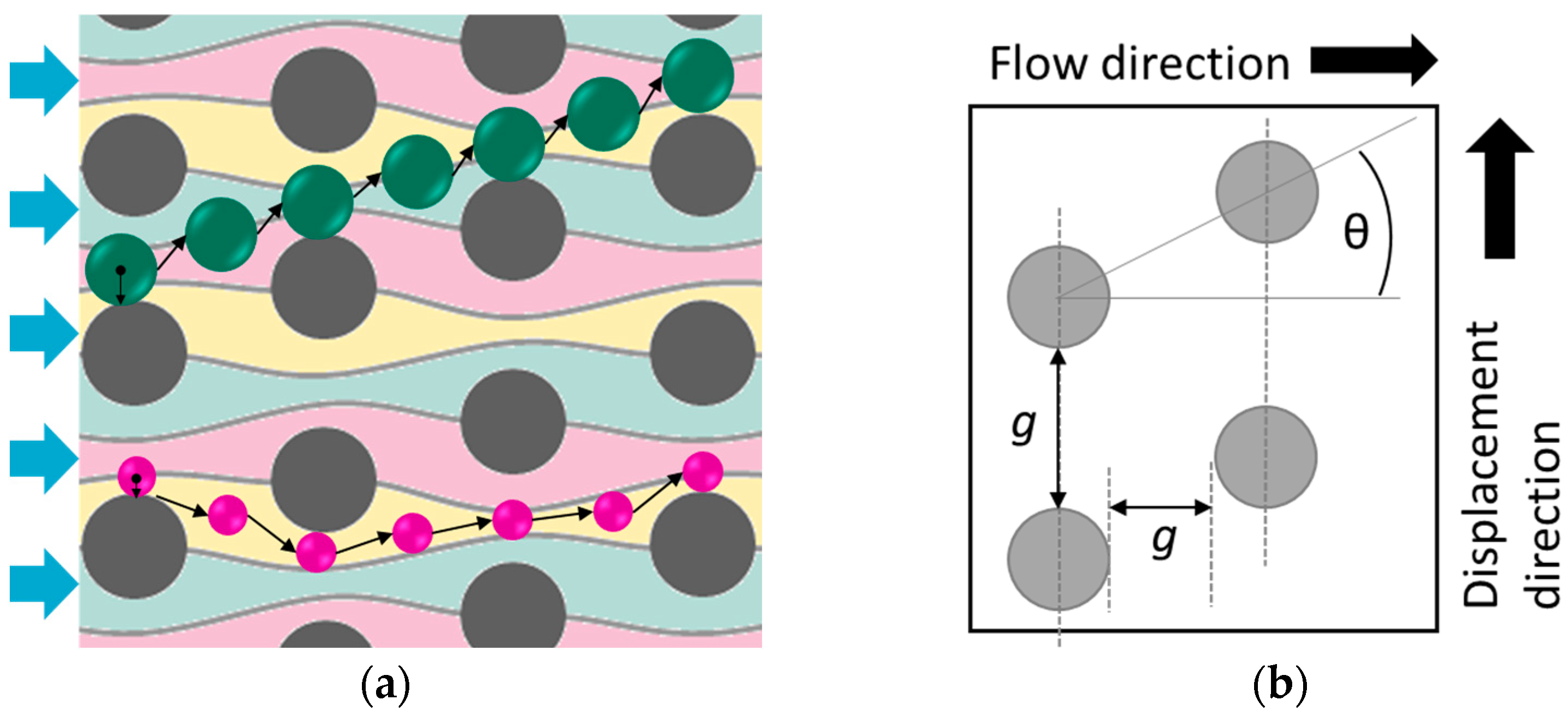
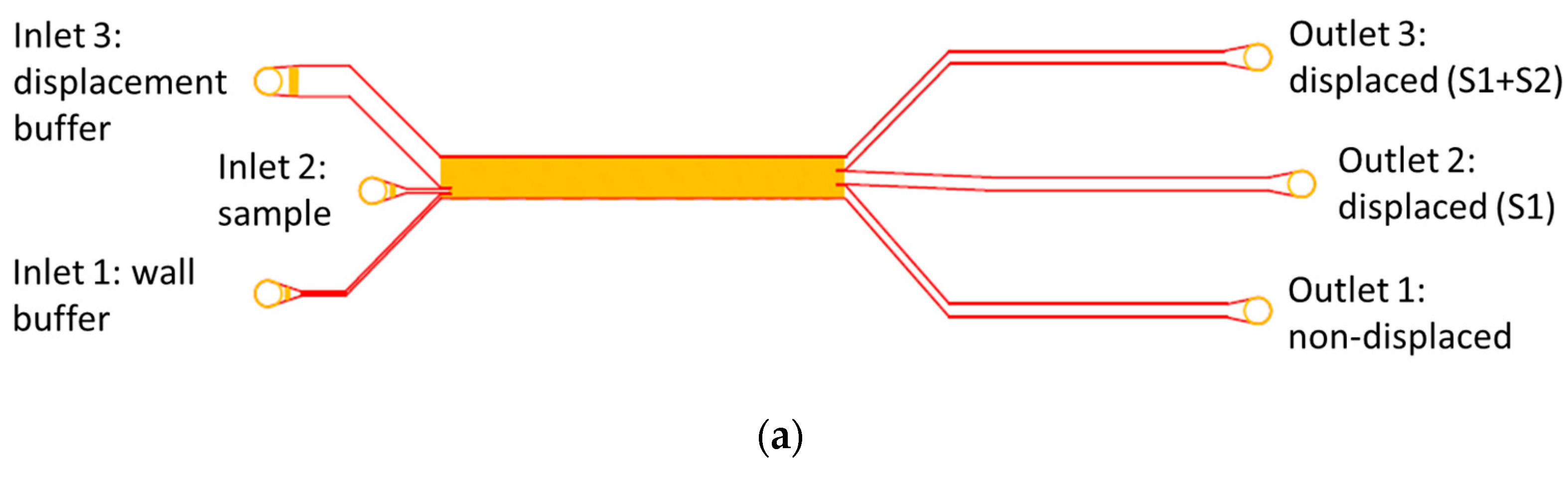
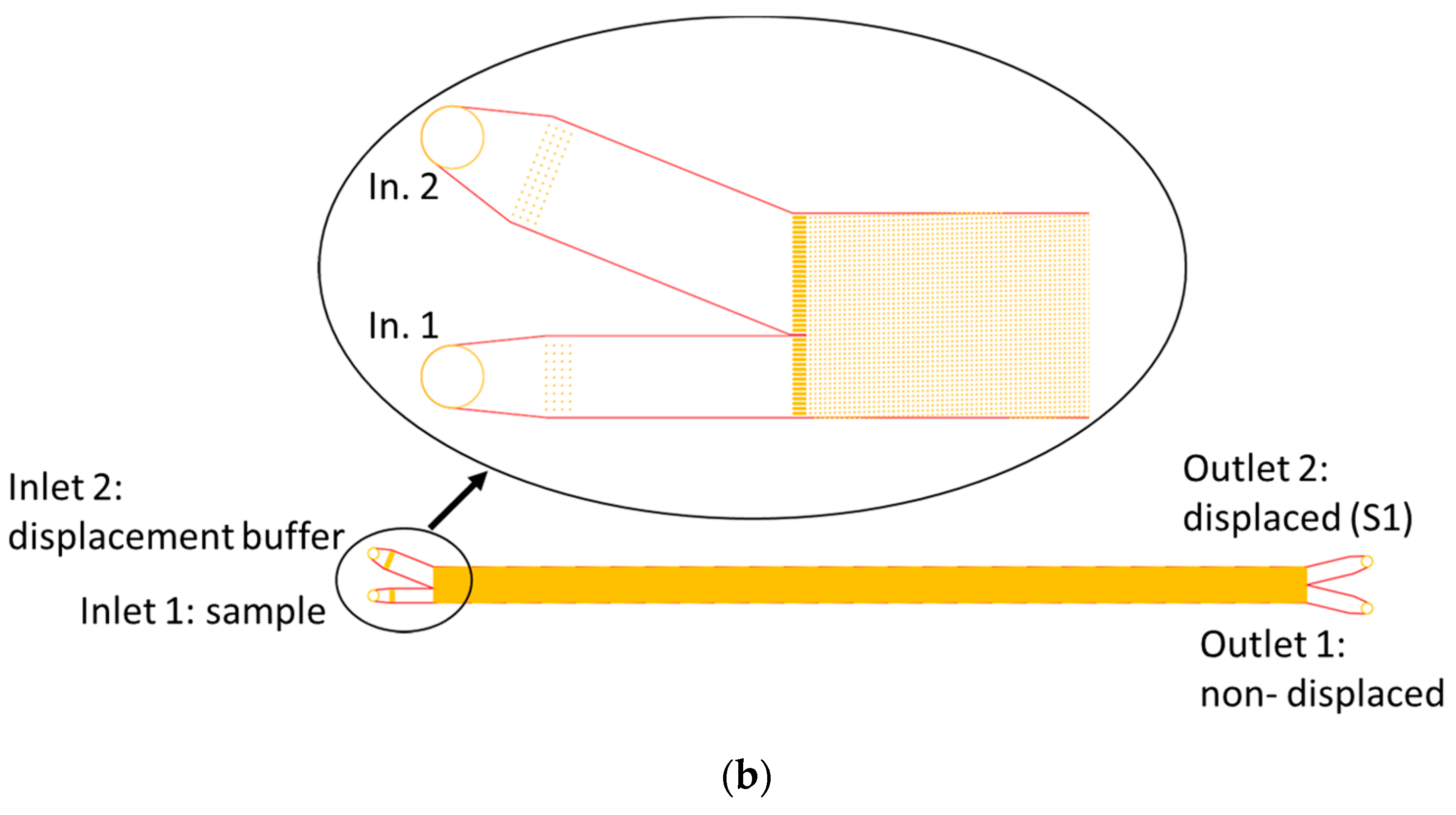
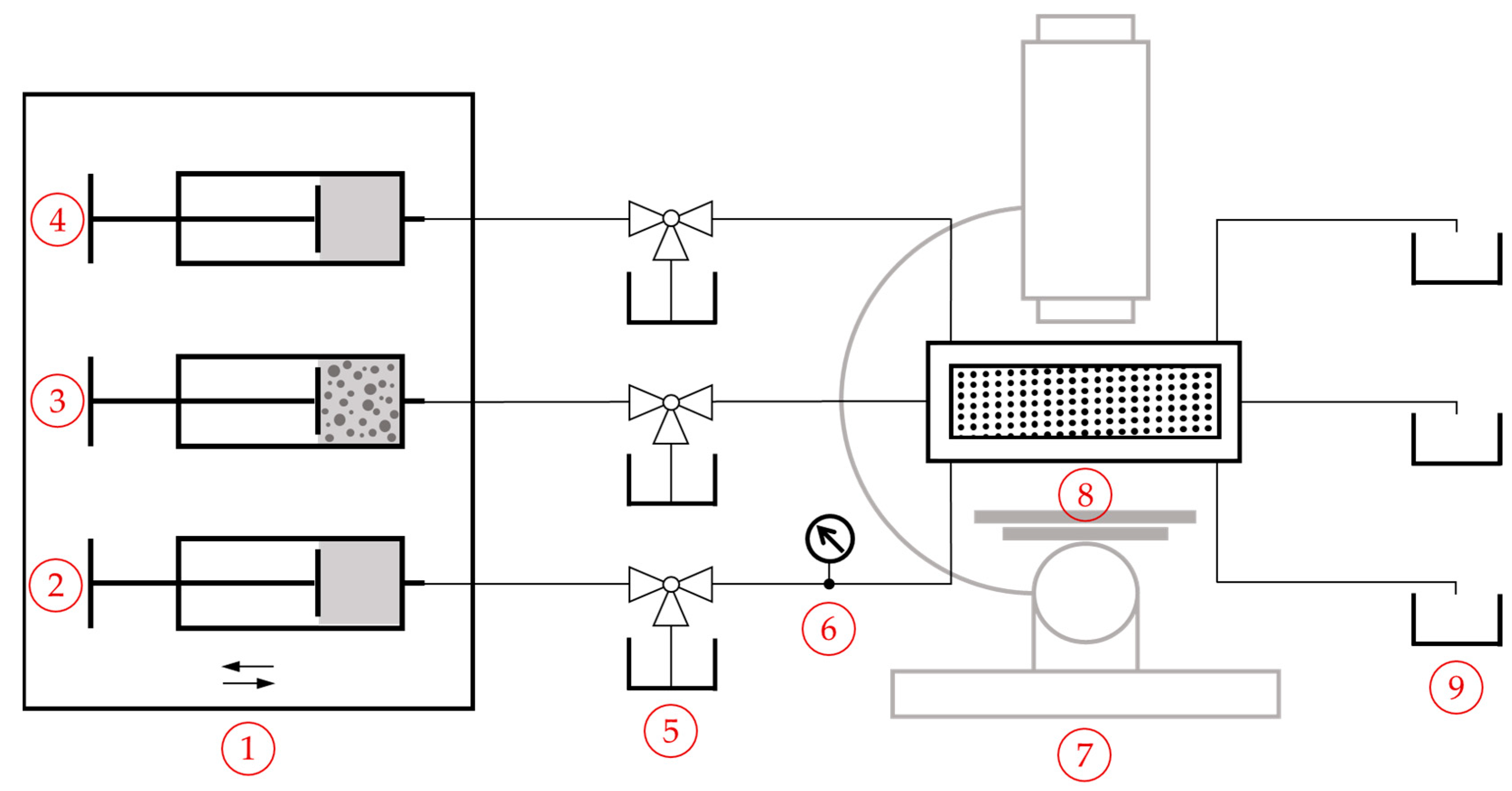
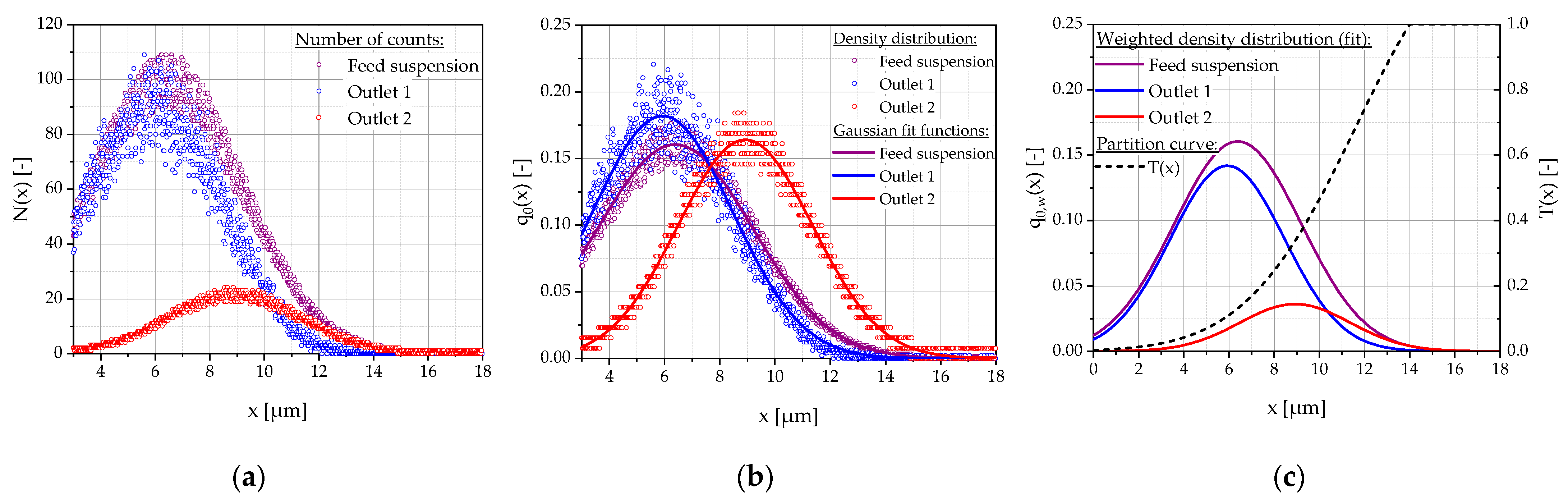
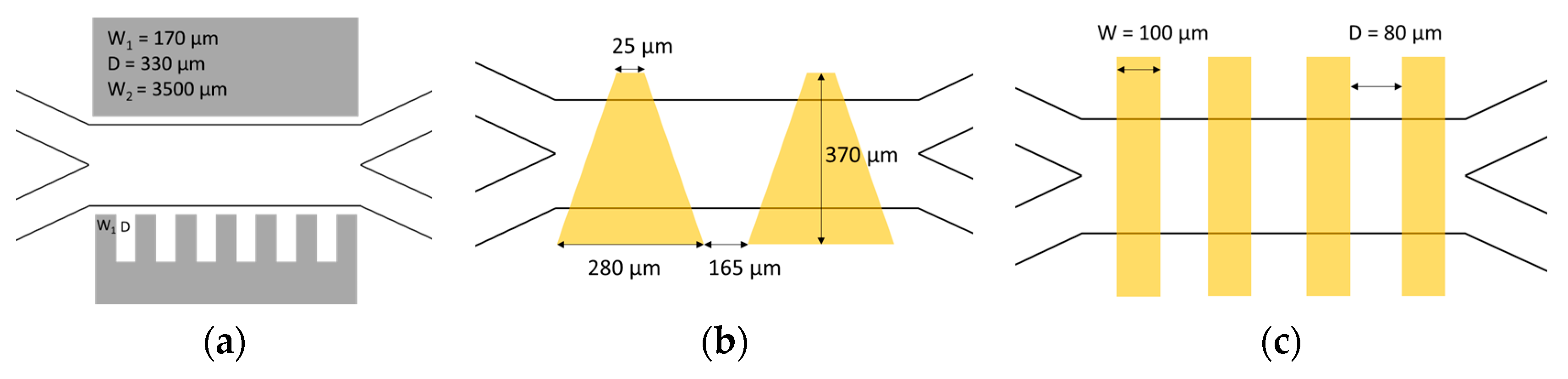

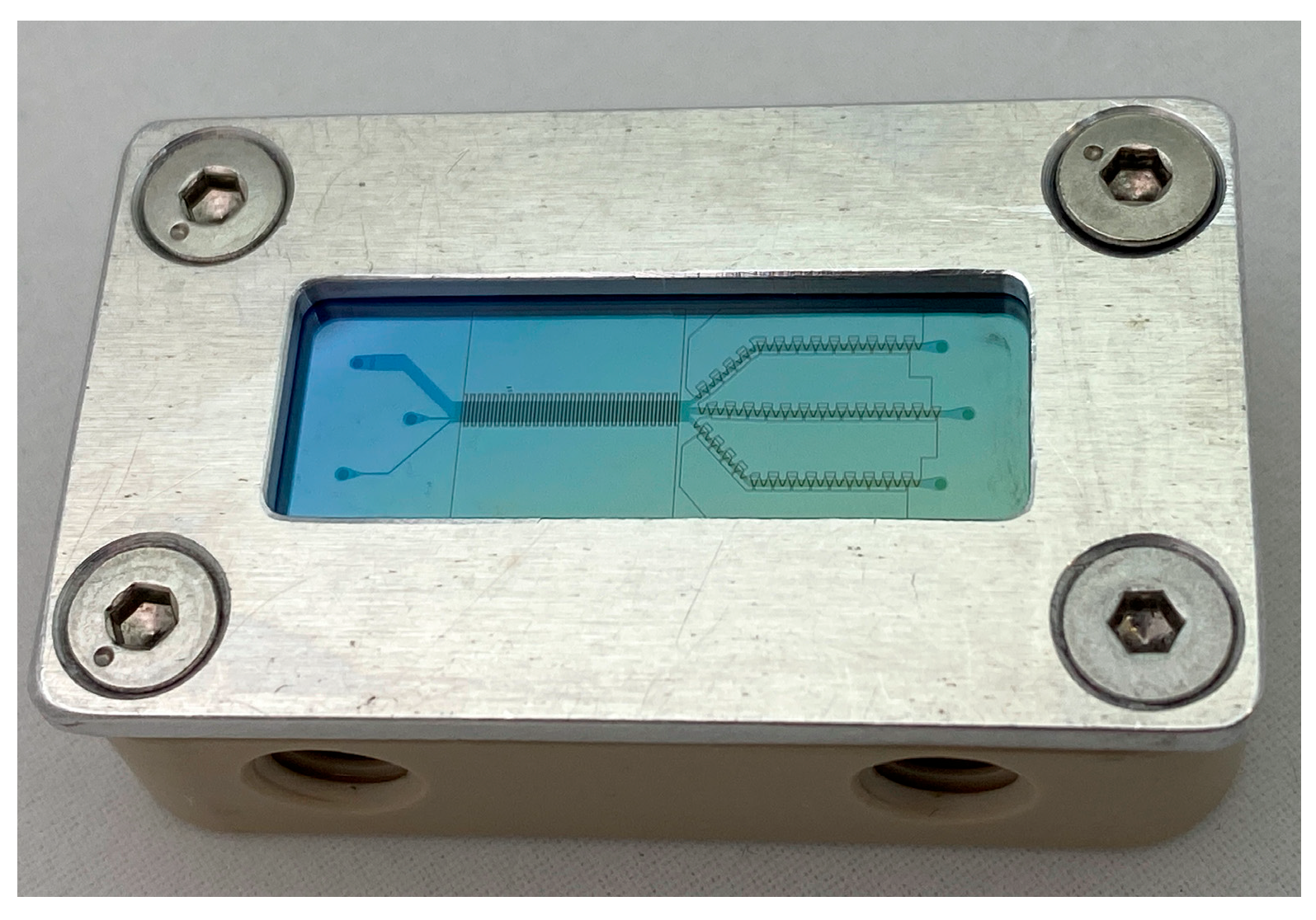
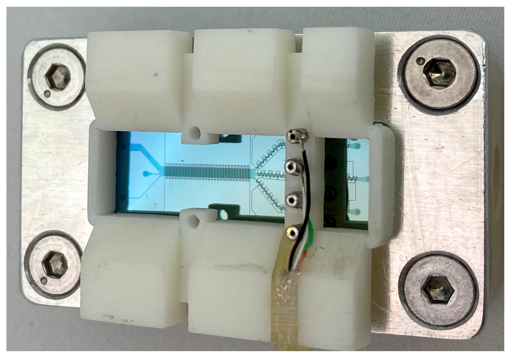
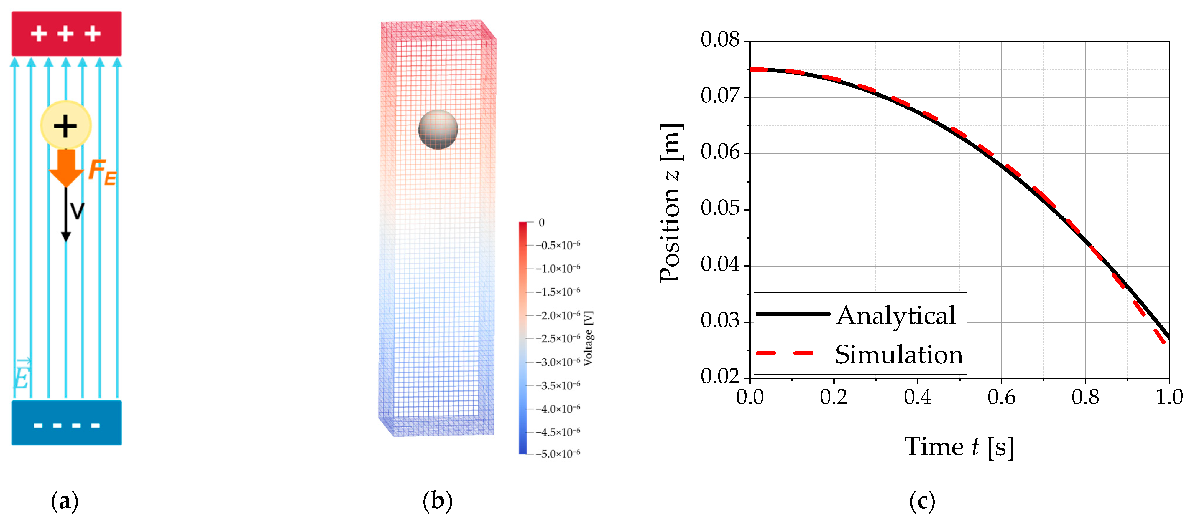
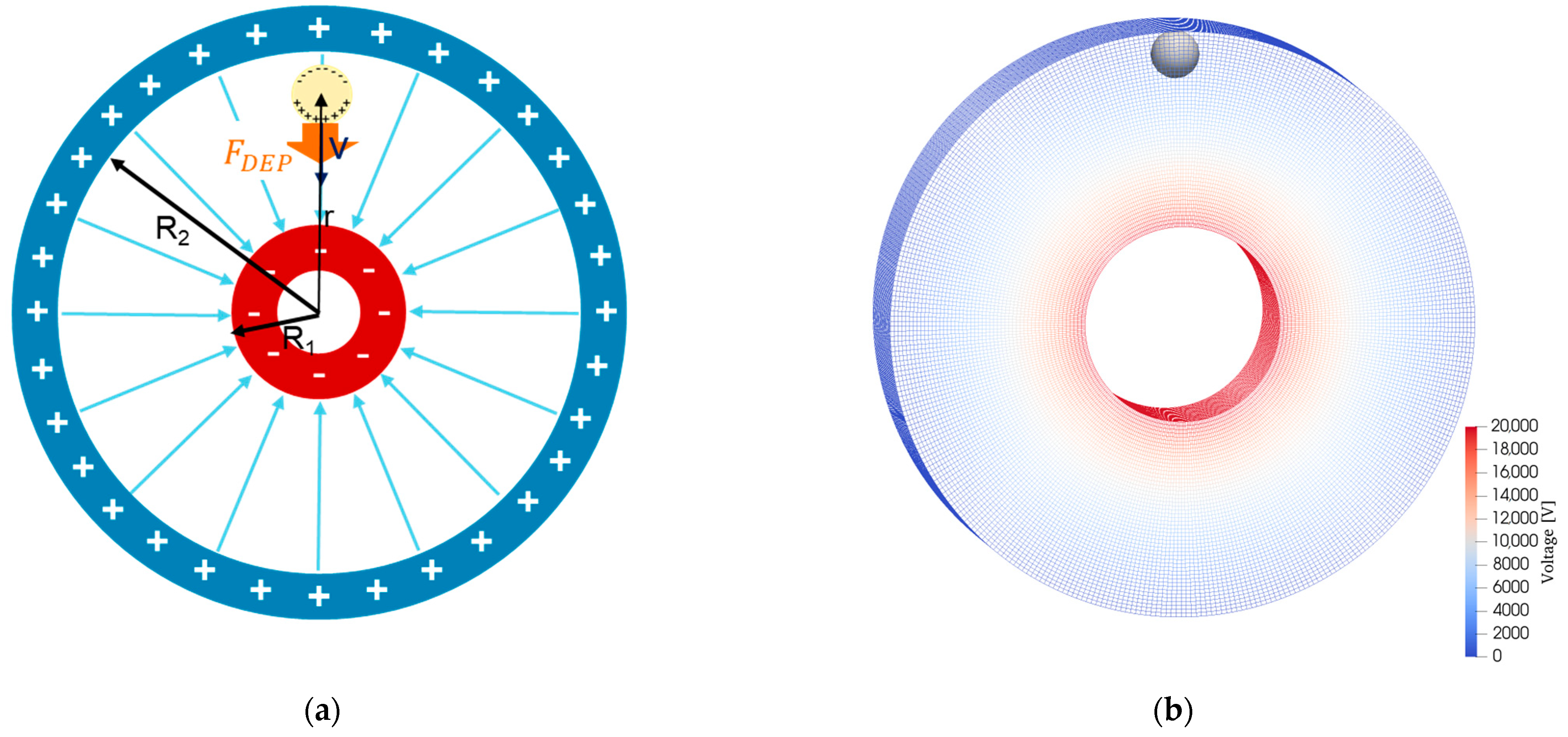

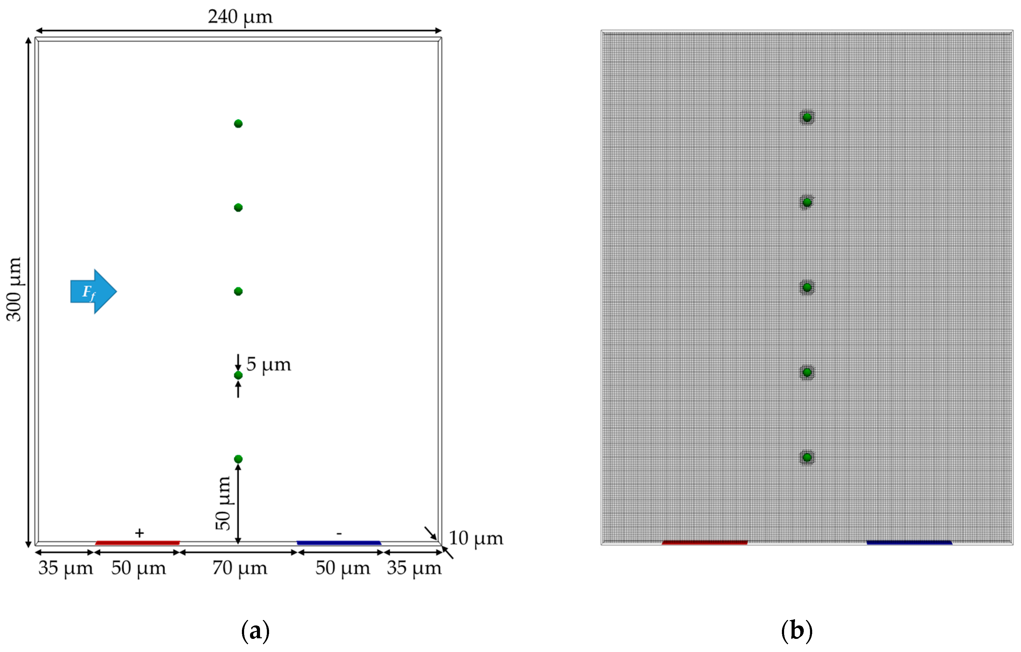
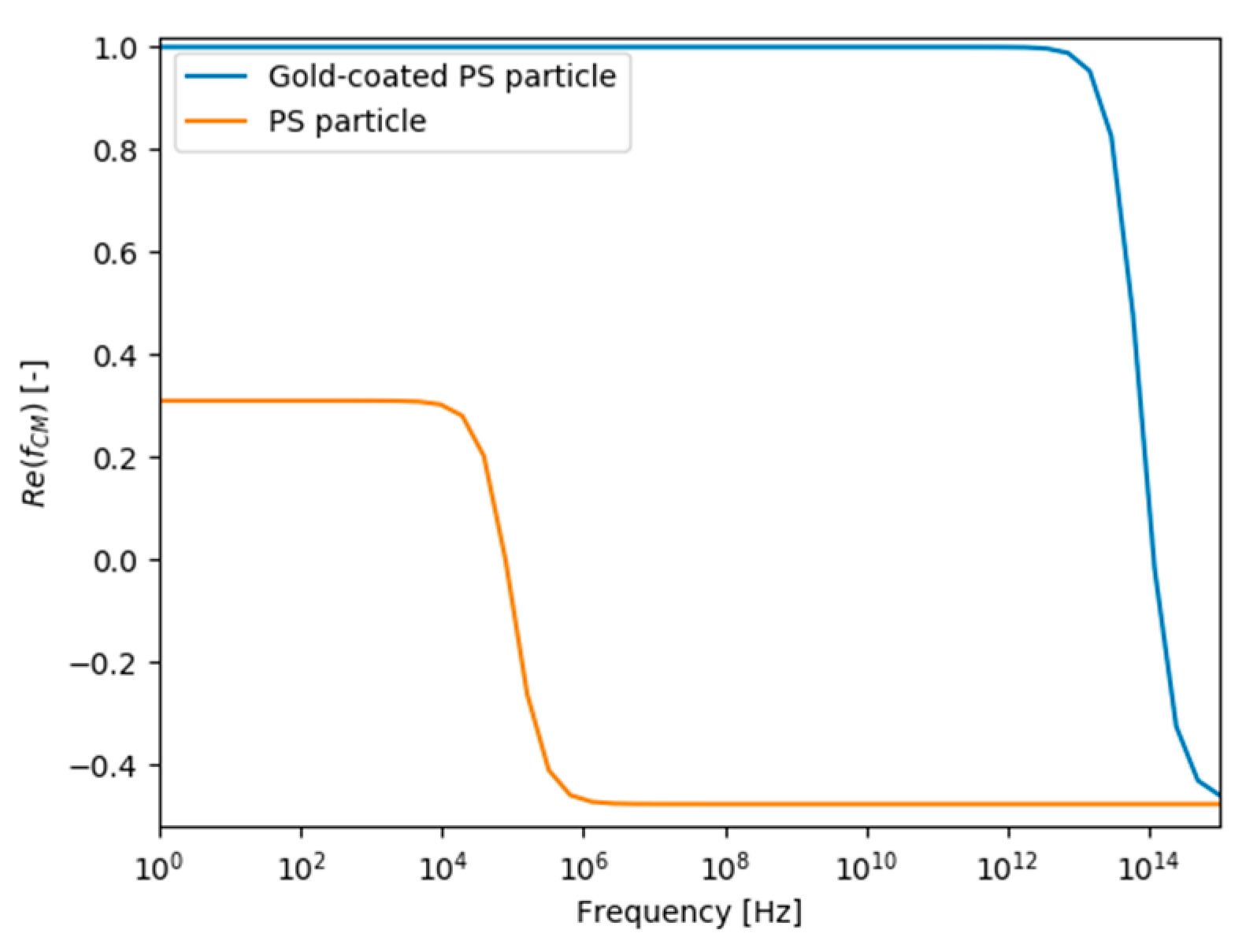

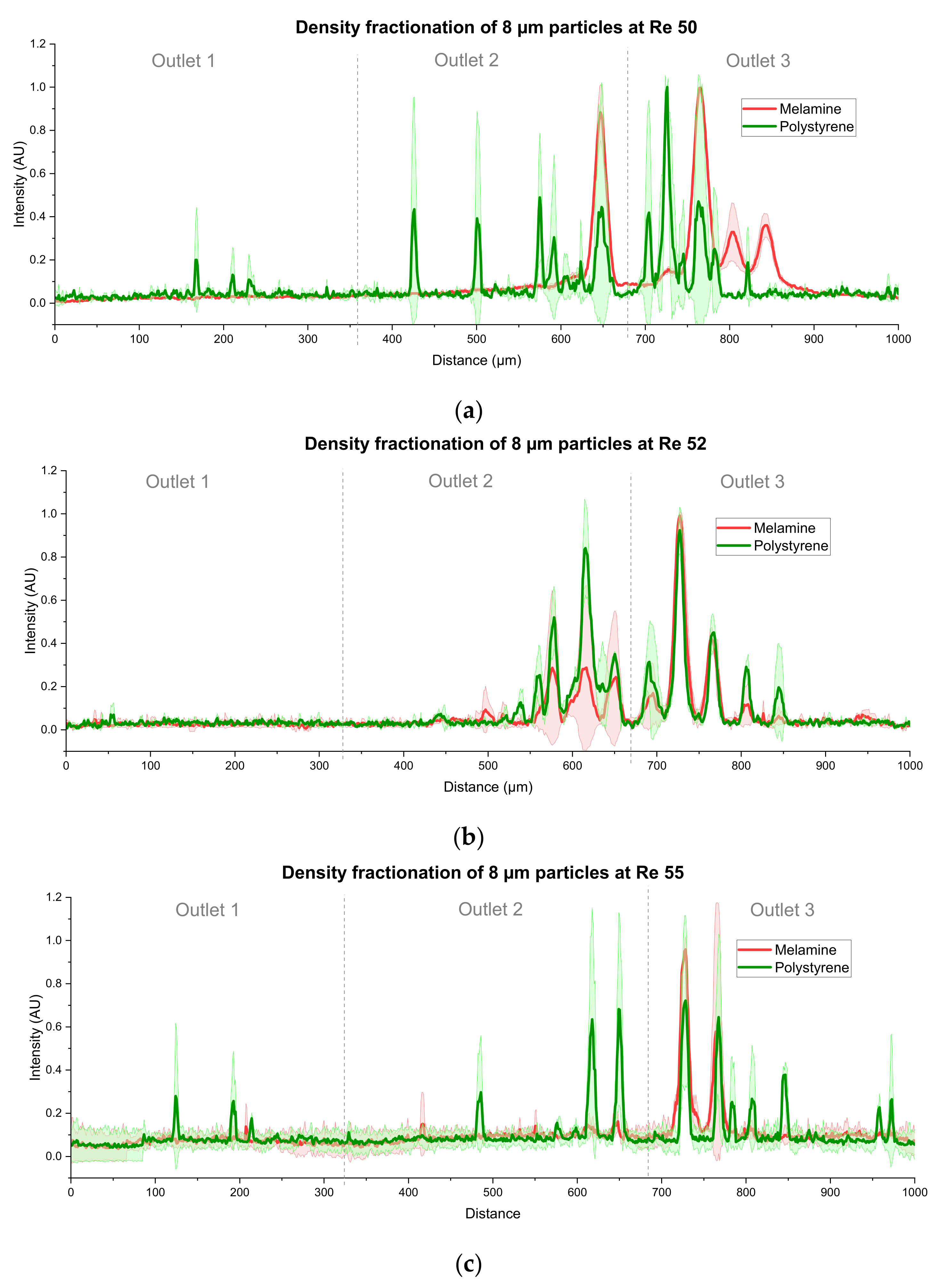
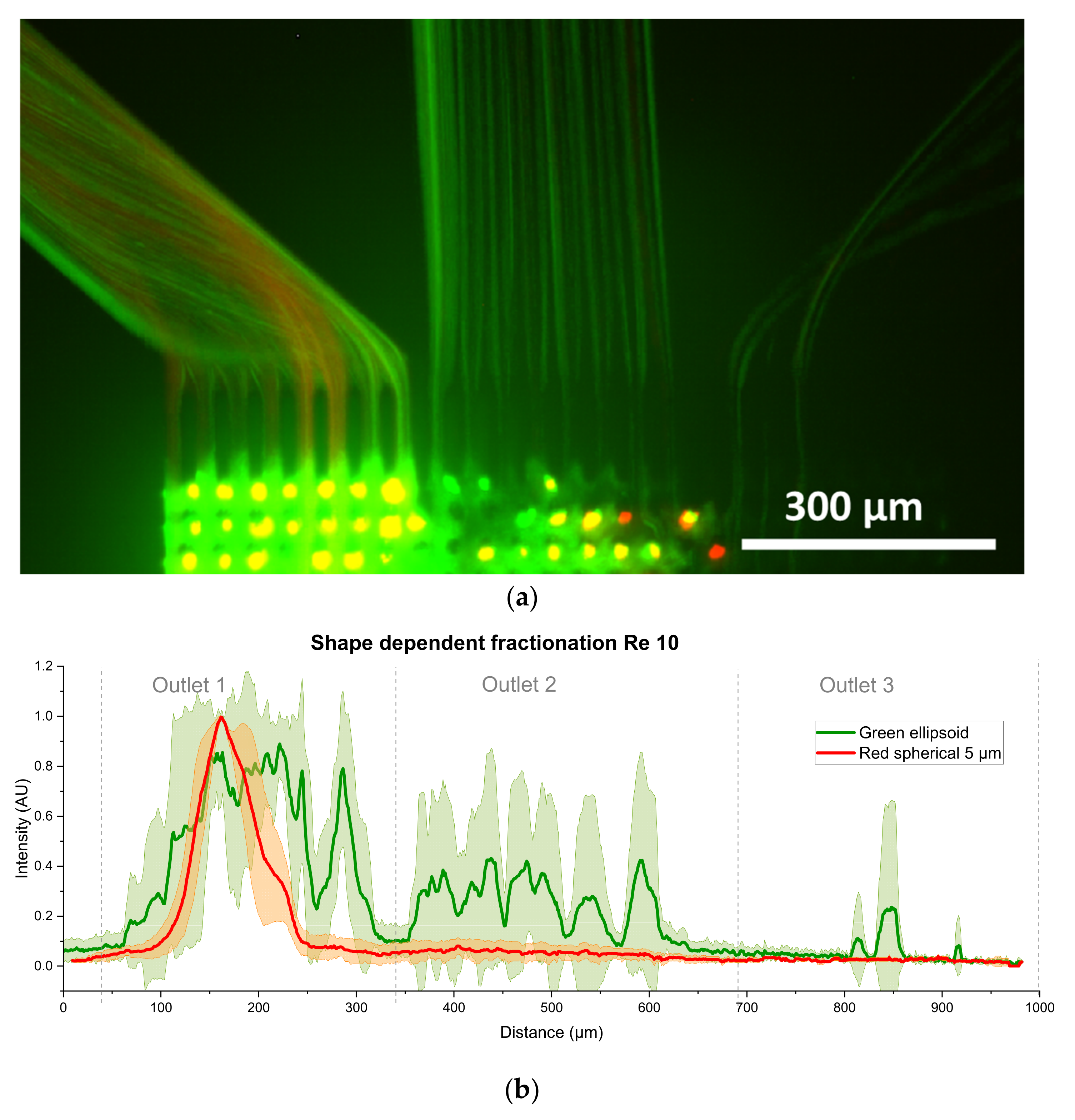
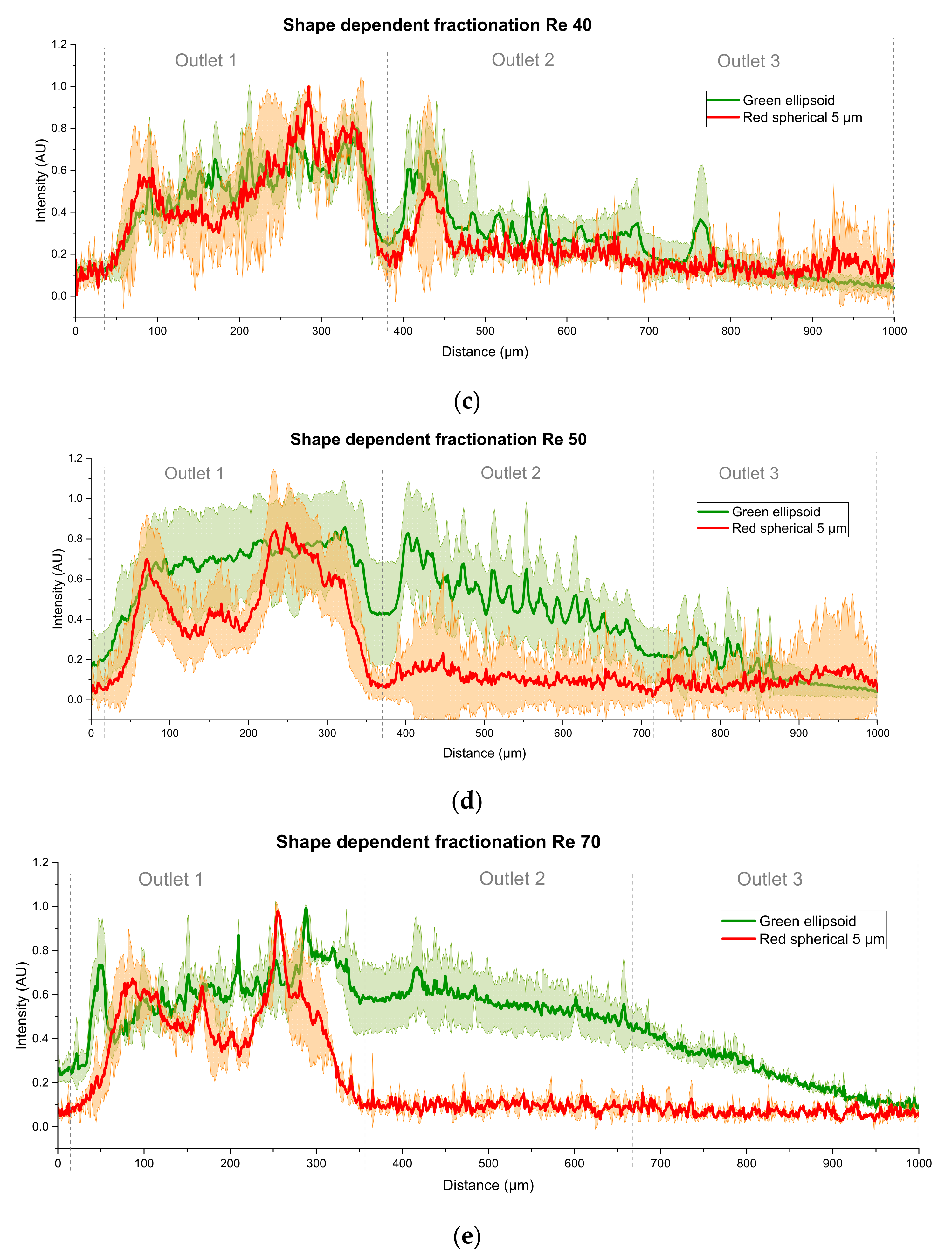

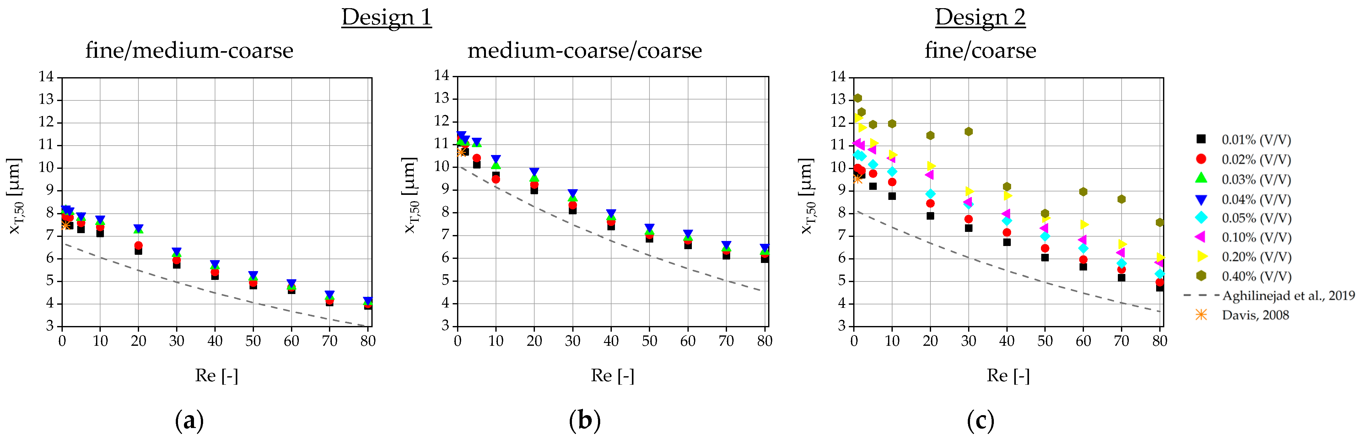
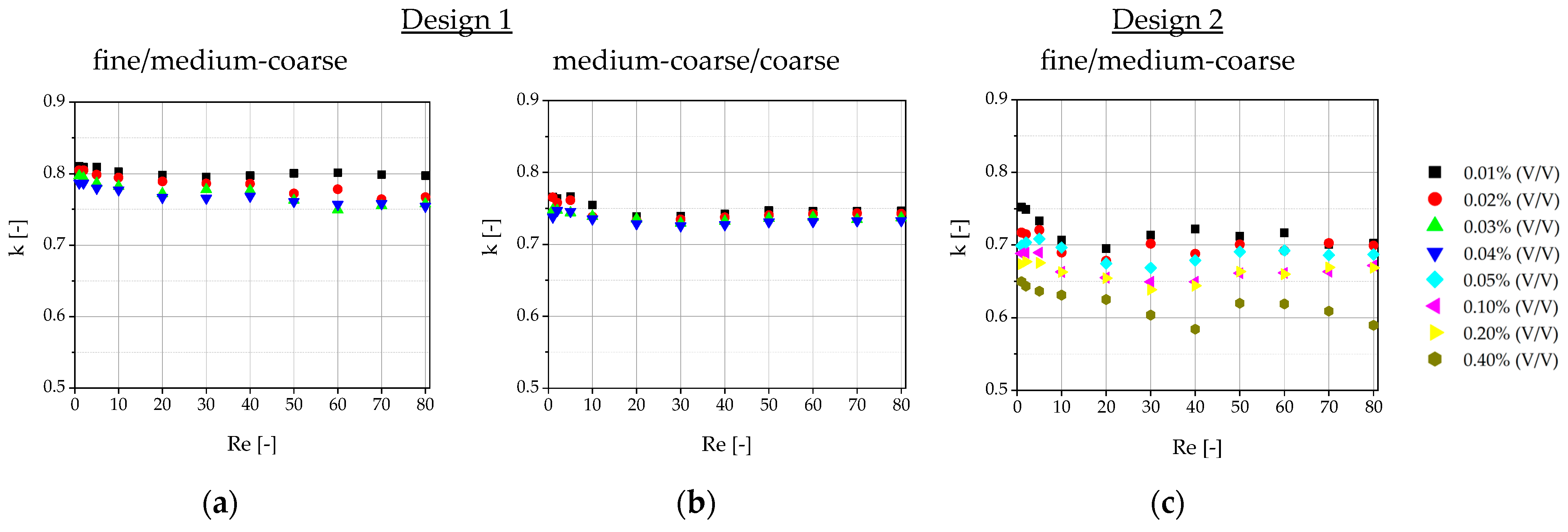

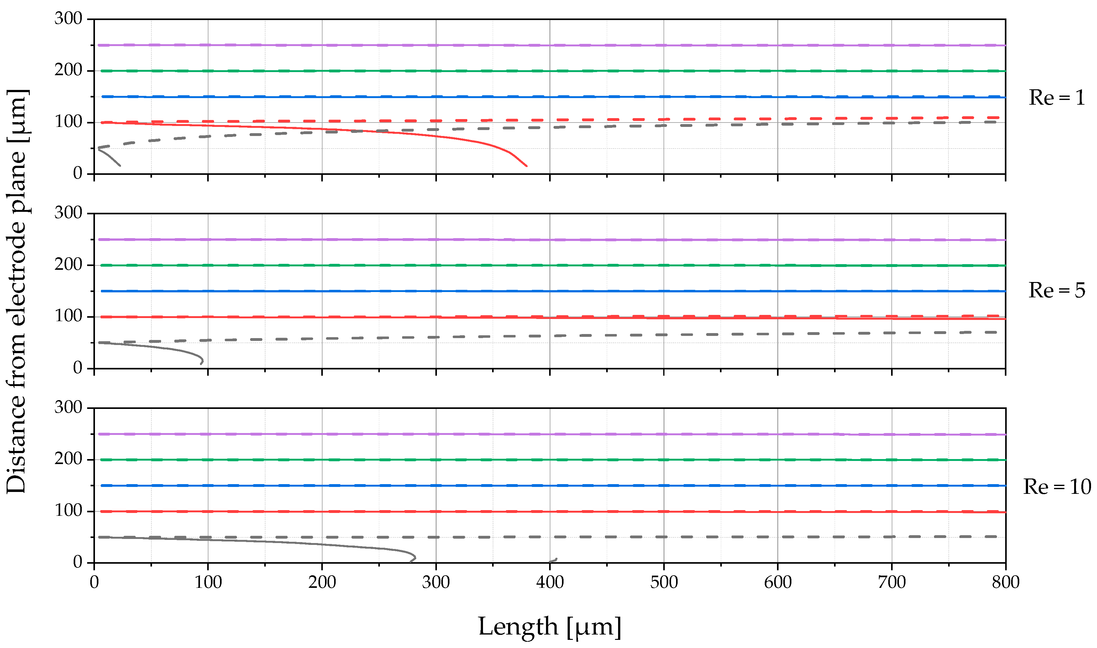
Disclaimer/Publisher’s Note: The statements, opinions and data contained in all publications are solely those of the individual author(s) and contributor(s) and not of MDPI and/or the editor(s). MDPI and/or the editor(s) disclaim responsibility for any injury to people or property resulting from any ideas, methods, instructions or products referred to in the content. |
© 2025 by the authors. Licensee MDPI, Basel, Switzerland. This article is an open access article distributed under the terms and conditions of the Creative Commons Attribution (CC BY) license (https://creativecommons.org/licenses/by/4.0/).