Article

Centrifugal Differential Mobility Analysis—Validation and First Two-Dimensional Measurements

by
Torben Norbert Rüther
,
Sebastian Gröne
,
Christopher Dechert
and
Hans-Joachim Schmid
*
Particle Technology Group, Department Mechanical Engineering, Paderborn University, Warburger Straße 100, 33098 Paderborn, Germany
*
Author to whom correspondence should be addressed.
Powders 2025, 4(2), 11; https://doi.org/10.3390/powders4020011
Submission received: 4 January 2025 / Revised: 12 March 2025 / Accepted: 26 March 2025 / Published: 2 April 2025

Abstract

:
To obtain a more comprehensive understanding of the specific properties of complex-shaped technical aerosols—such as partially sintered aggregates formed in combustion processes or structured particles resulting from complex synthesis processes—it is essential to measure more than a single equivalent size. This study examines a novel method for determining a two-dimensional distribution of two distinct particle properties within the size range from 50 nm to 1000 nm : the Centrifugal Differential Mobility Analyzer (CDMA). The CDMA enables the simultaneous measurement of both mobility and Stokes equivalent diameters, providing a detailed two-dimensional particle property distribution. This, in turn, allows for the extraction of shape-related information, which is essential for characterizing particles in terms of their chemical composition, reactivity, and other physicochemical properties. This paper presents a detailed evaluation of a first CDMA prototype. First, CFD simulations of the flow field within the classifier are presented in order to assess and understand non-idealities arising from the exact geometry. Subsequently, the transfer function is evaluated by particle trajectory calculations based on the simulated flow field. It can be demonstrated that the simulated transfer functions agree quite well with transfer functions derived from streamlines of an ideal flow field, indicating that the non-idealities in the classifying region are almost negligible in their effect on the classification result. An experimental determination of the transfer function shows additional effects not covered by the previous simulations, like broadening by diffusion and losses due to diffusion and precipitation within the in- and outlet of the classifier. Finally, the determined transfer functions are used to determine the full two-dimensional distribution with regard to the mobility and Stokes equivalent diameter of real aerosols, like spherical particles and aggregates at different sintering stages, respectively.

1. Introduction

Technical aerosols often exhibit complex behavior influenced by particle size, structure and shape. Characterizing such ensembles, particularly in the case of nanoscale aerosols, presents significant challenges, as their small dimensions severely limit the investigation through conventional light scattering techniques [1,2]. For aggregates with highly intricate and irregular morphologies, defining a single representative particle size becomes even more difficult [2,3]. Consequently, in most cases, an equivalent property is introduced as a practical means of characterization.
An equivalent diameter is defined as the diameter of a spherical particle that exhibits the same specific property (such as electrical mobility, inertial behavior, or settling velocity) as the particle under consideration. However, relying solely on a single equivalent diameter is inherently insufficient for a comprehensive characterization of complex particle properties, as it does not capture variations in shape, structure, or composition. To achieve a more detailed and accurate characterization, it is essential to assess multiple properties or equivalent diameters. One approach to obtaining such information is through electron microscopy, which provides structural insights, at least in the form of a projection area. This allows for a more refined analysis of particle morphology and enables a better understanding of their physical and chemical behavior.
Furthermore, so-called tandem configurations enable the measurement of two-dimensional distributions of different equivalent particle sizes, providing a more detailed characterization of aerosol properties. These setups consist of a sequential arrangement of two instruments: the first serves as a classifier, selectively isolating a specific fraction of particles based on one equivalent size, while the second either measures an additional property of the classified aerosol or performs a secondary classification based on a different equivalent size. By combining these two measurement stages, tandem configurations offer deeper insights into particle characteristics, allowing for a more comprehensive analysis of their morphology, composition, and dynamic behavior. Park et al. [4] employed a DMA-APM (Dynamic Mobility Analyzer-Aerosol Particle Mass Analyzer) configuration to simultaneously measure two different equivalent diameters. This approach was later utilized by Rawat et al. [5] to calculate a two-dimensional distribution. Since then, data inversion models for 2D distributions have been widely adopted and applied to various tandem measurement configurations [6,7]. Broda et al. [8], for instance, implemented a Twomey algorithm to derive a 2D distribution function for the mass concentration of carbon black using a CPMA-SP2-CPC (Centrifugal Particle Mass Analyzer–Single Particle Soot Photometer–Condensation Particle Counter) setup. Moreover, Sipkens et al. [9] published a comprehensive review discussing various measurement techniques for carbon black and their applications in tandem configurations.
However, these tandem methods are inherently complex. Specifically, they necessitate at least two separate devices, which increases the overall cost of the setup. Furthermore, such configurations demand a high level of specialized knowledge and technical proficiency to conduct and evaluate such measurements. The complexity arises from the unique nature of these setups, which require users to possess a deep understanding of the underlying principles and operational intricacies. Additionally, for each specific setup, the data inversion process must either be developed from scratch or adapted by the user, adding another layer of technical demand. This combination of cost, complexity and user expertise highlights the challenges associated with utilizing tandem measurement methods in aerosol characterization. Furthermore, when using two classifiers in tandem, the resulting particle concentration at the exit is typically very low. This is due to the convolution of both transfer functions, which leads to a significant reduction in the number of particles that pass through both classifiers. As a consequence, the statistics of the resulting size distributions may be poor, often requiring either significantly longer measurement times or resulting in unreliable data. To address these limitations and enable the simultaneous measurement of multiple particle properties, the CDMA (Centrifugal Differential Mobility Analyzer) was developed. The CDMA integrates the principle of classification of an Aerodynamic Aerosol Classifier (AAC) [10] with that of a Differential Mobility Analyzer (DMA) [11] in one single instrument. This allows for the measurement of a true two-dimensional distribution of both the equivalent mobility diameter and the equivalent Stokes diameter. Furthermore, additional parameters, such as effective density and fractal dimension, can be derived from this approach, providing valuable insights into particle shape and structure [4,12,13]. These additional characteristics further enhance the comprehensiveness of the analysis, enabling a more detailed analysis of aerosol particles in terms of their physical and morphological attributes.
The principle of the CDMA, the design of a first prototype and an idealized transfer function, alongside a method for measuring the transfer function that facilitates the determination of its parameters have been published recently in a first paper [14]. Building upon this, a second paper thoroughly examined the theoretical transfer functions of the CDMA. Various alternative approaches were compared, while the influence of diffusion and applied boundary conditions on the system’s behavior was also investigated [15]. A third paper focused on the application of the Projection Onto Convex Sets (POCS) algorithm for data inversion. The algorithm which had not been used before in the context of particle characterization was tested with both experimental and idealized datasets, and its performance was critically assessed [16].
The present work now substantially extends the findings from these previous publications. In particular, results from a flow-field simulation inside the classifier are presented and non-idealities in the flow field are discussed in detail. Subsequently, a method to simulate the transfer function based on particle trajectory simulations using the simulated flow fields is presented. Furthermore, the resulting transfer functions are compared to results from a much simpler streamline approach based on an idealized flow field. This reveals the influence of the flow non-idealities on the classification result. Furthermore, a methodology to measure the overall transfer function of the CDMA prototype is applied and the resulting transfer functions dependent on particle size and the flow ratio are extensively studied. Finally, the CDMA is used to characterize real aerosols of silver nanoparticles. In particular, aggregates of different structures resulting from different sintering stages are characterized by their full 2D structures to comprehensively characterize complex particles.

2. Theoretical Fundamentals
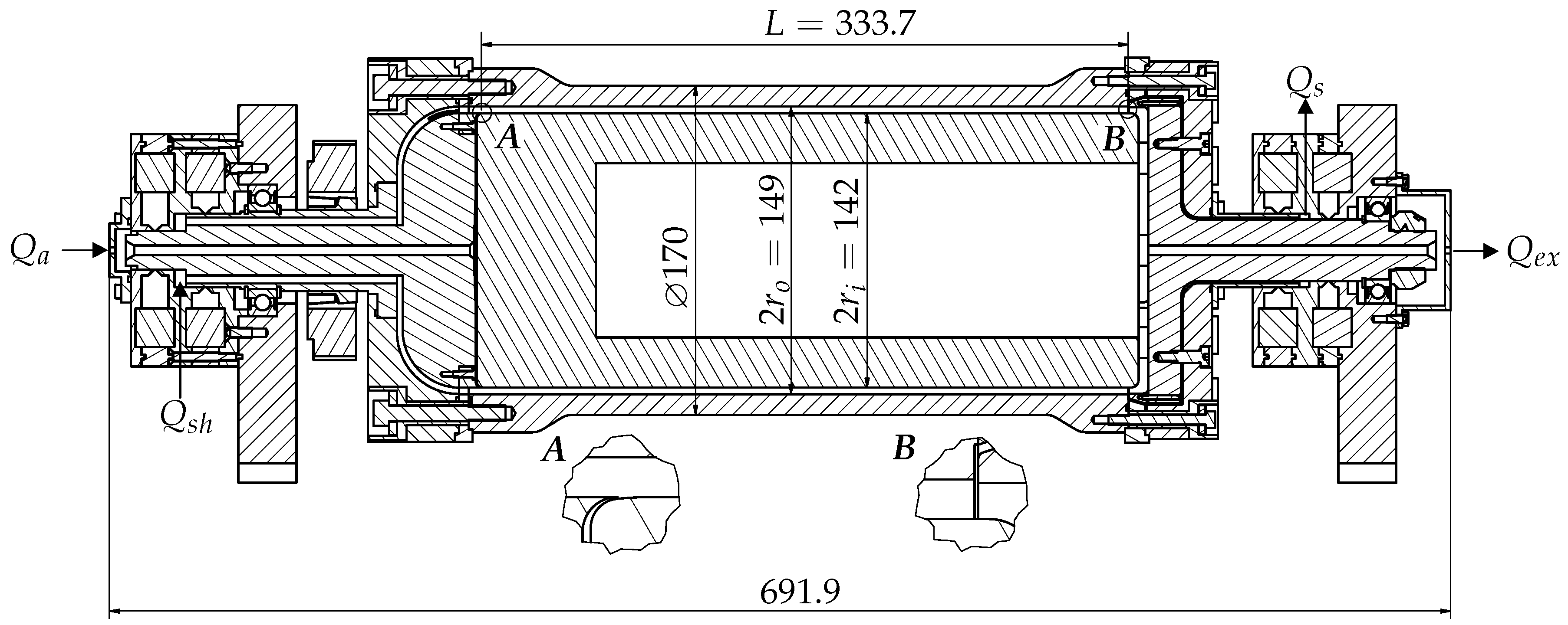
As extensively described in Rüther et al. [14], the CDMA shares key similarities with both the DMA and the AAC. Therefore, the CDMA is composed of two concentric cylinders that form a cylindrical gap, through which a sheath airflow is directed (see cross-section of the CDMA in Figure 1). These cylinders are electrically isolated from one another, enabling a voltage to be applied between them, in line with the operational principle of the DMA. Additionally, both cylinders can be rotated at the same angular velocity, following the operational principle of the AAC. This design integrates the core features of both instruments, enabling the simultaneous measurement of multiple particle properties. When an aerosol volume flow is applied to the inner cylinder (c.f. Figure 1, detail A), the particles are moved through the sheath air towards the outer cylinder by electrical and/or centrifugal forces. At the end of the classification chamber, (c.f. Figure 1, detail B), the particles are sampled, so that particles matching the predetermined properties are extracted as sample volume flow for subsequent particle counting.
Assuming Stokes’ drag force and neglecting inertia, the force equilibrium results in:
Q P · E + m P · a c = 3 π η d m w D r · 1 C u ( d m )
Q P represents the particle charge, E = U r · ln ( r o / r i ) denotes the electric field strength in a radial direction, m P is the particle mass, a c = ω 2 · r represents the centrifugal acceleration, η denotes the dynamic viscosity, d m is the mobility diameter, w D r denotes the radial particle drift velocity, and C u is the Cunningham slip correction factor [17]. The deterministic description of the particle path neglecting diffusion is achieved by rearranging and integrating Equation (1).
r x = τ · ω 2 · r i n 2 + Z · U ln r o r i · exp 2 · τ · ω 2 · x · π · r o 2 r i 2 Q s h + Q a Z · U ln r o r i τ · ω 2
U represents the voltage applied to the outer cylinder, ω denotes the rotational velocity of both cylinders, r o and r i are the outer and inner radii, r i n is the radius at which the particle enters into the classification gap, x is the position of the particle in the axial direction, Q s h is the sheath air volume flow, Q a is the aerosol volume flow, τ is the particle relaxation time and Z is the particle mobility. With
τ = ρ · d v 3 · C u ( d m ) 18 · d m · η = ρ · d s t 2 · C u ( d m ) 18 η
and
Z = n · e · C u ( d m ) 3 π · η · d m
with ρ as the particle density, d v as the volume equivalent diameter, d s t as the Stokes equivalent diameter, n as the number of charges carried by a particle, and e as the elementary charge. Please note that n and U might be positive or negative depending on the polarity and charge, respectively. Also note that, according to Rüther et al. [14], the argument of the Cunningham slip correction factor is d m .
Therefore, the trajectory of a particle with given properties d m and d s t can be calculated from the volume flow ratio and the applied rotational velocity and voltage.
Z * is the mobility required for a particle entering at the center of the aerosol inlet to be sampled exactly at the center of the outlet for a given set of operational parameters [18]. τ * describes the same behavior but for the relaxation time [10].
Z * = Q s h + Q e x 4 · π L U · ln r o r i
τ * = Q s h + Q e x π ω 2 ( r i + r o ) 2 L
with Q e x being the excess volume flow and L the length of the classifying gap. Relating the particle properties Z and τ to the characteristic values at the actual operation point Z * and τ * lead to the normalized mobility or the normalized particle relaxation time, respectively.
Z ˜ = Z / Z * ; τ ˜ = τ / τ *

3. Design

Figure 1 shows the cross-section of a first prototype of the CDMA. The aerosol is fed from the left side, enters through the center bore, and flows through a small gap to the inlet of the classification region A. The sheath air is fed between two ferrofluidic seals on the left side. Then, it passes through eight axial holes into the CDMA. After a flow deflection, the sheath air also enters into the classification gap at A. Together the flows pass through the classification zone. At point B, the excess volume flow continues the inner cylinder, flows to the center and exits through a center bore on the right side. The sample air is extracted in the radial direction at point B. Then, the sample flows through small channels until it leaves the CDMA through a small hole between the ferrofluidic seals on the right side. Voltage can be applied through a carbon-sliding contact on the outer cylinder, the rotational speed is applied by a belt drive mounted on the left side. For more details about the design of the CDMA prototype, see also [14].

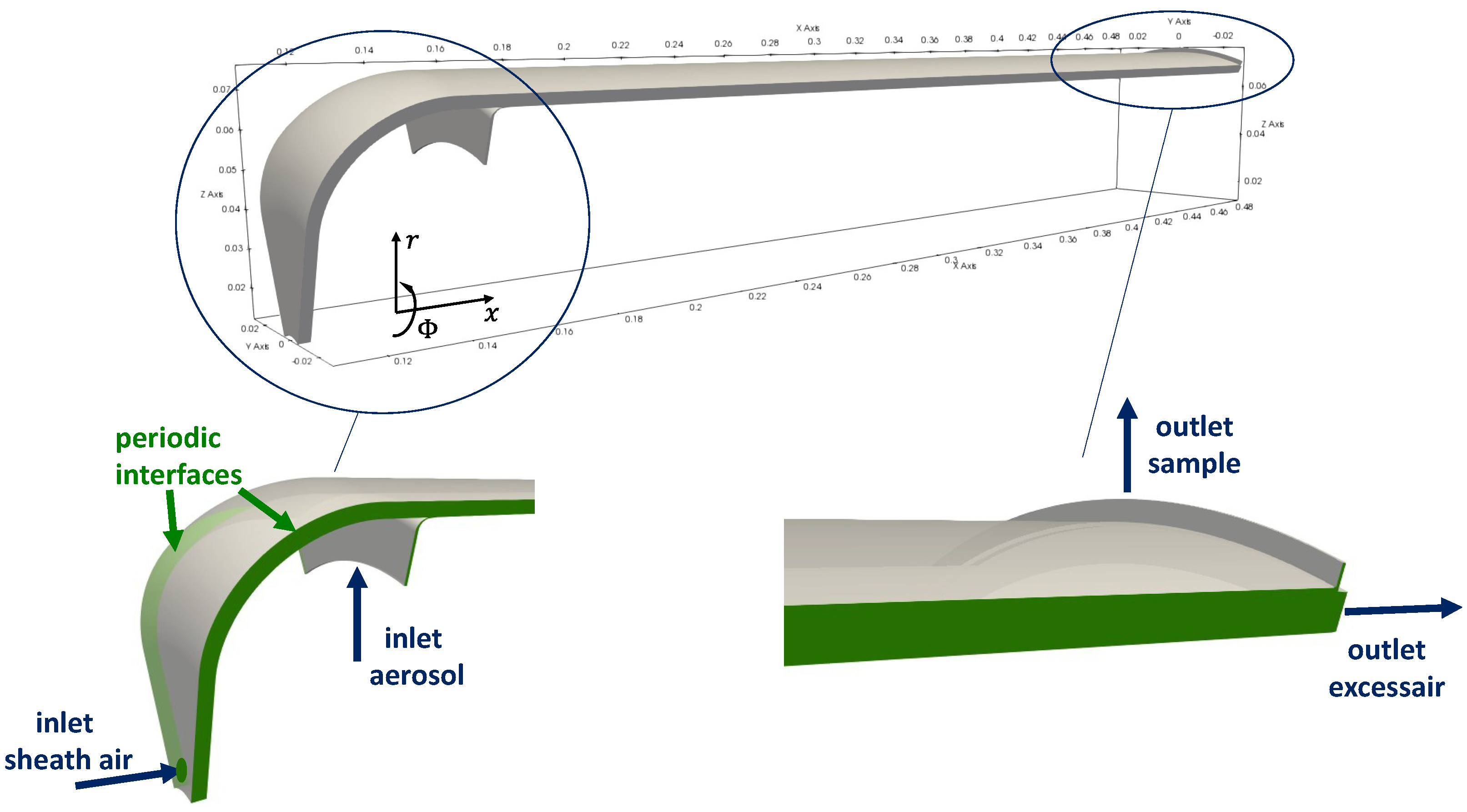
4. Numerical Flow Simulations

CFD simulations were performed in order to verify the flow profile in the classification gap and to identify potential non-ideal flow patterns. A simulation was performed using the OpenFOAM Version 8 framework under the assumptions of incompressible and isothermal flow, employing the k ω SST turbulence model [19]. Although the results indicated laminar flow within the classifying gap, this turbulence model was selected to ensure an accurate representation of potential turbulence in the inlet and outlet regions. Moreover, due to the presence of narrow gaps, the k ω SST model was preferred over the k ϵ model, as it exhibits superior performance in wall-bounded flows, particularly within the viscous sublayer. Although the k ω model tends to overestimate shear stress in fluid flows, the k ω SST model mitigates this by incorporating the k ϵ model in regions away from the walls. By analyzing the turbulent kinetic energy, critical regions can be identified and subsequently examined for the presence of micro-vortices in potential future studies using Large Eddy Simulation (LES) or Direct Numerical Simulation (DNS). Surface roughness is not considered in this work due to the surface being highly polished and the predominant laminar flow characteristics.
In the simulation, pure particle-free air under standard conditions is used as the working fluid. The sheath air is introduced through eight symmetrically arranged inlet tubes (indicated by the green dot in Figure 2) and is subsequently distributed uniformly along the entire circumference. Within the computational model, these inlets are represented as laminar flow profiles entering the simulation domain. To optimize computational efficiency, the flow domain is reduced to a representative angular section of 45 ° in the circumferential direction, as illustrated in Figure 2. This reduction is justified by the symmetry of the system, allowing for an accurate representation of the overall flow behavior while minimizing computational cost.
At the symmetry interfaces, periodic boundary conditions are applied, so that fluxes across the interfaces are admitted. The boundary condition at the walls is a zero-slip boundary condition (Dirichlet boundary condition for the velocity). The aerosol inlet, sheath air inlet, and excess air outlet are also set to a defined volumetric flow rate. A plug flow profile is assumed at the aerosol inlet and the excess air outlet, while a fully developed laminar tube flow is applied at the inlet of the sheath air. The sample outlet is defined by the Neumann condition; thus, the mass balance is always maintained.
The rotation is implemented by a single rotating frame approach, using the ‘SRFSimpleFoam’ solver to calculate the velocity fields. The computational grid consists of 70 elements in the radial direction, 50 elements in the circumferential direction, and 550 elements along the flow direction, with a logarithmically increasing resolution towards the boundary layers. A mesh independence study confirmed the adequacy of this resolution, as doubling the mesh density resulted in deviations of less than 0.4 % in the pressure drop across the prototype. Additionally, critical regions, such as the aerosol inlet and sample outlet, as well as edge areas, were refined to enhance the accuracy of the flow representation in these zones. This ensures a more precise depiction of localized flow phenomena and potential gradients.
The following simulation results are based on a flow ratio β = Q a / Q s h = 0.2 ( Q a = Q s = 0.3 l / min , Q s h = Q e x = 1.5 l / min ). The flow ratio β directly influences the width of the transfer function, with smaller β -values resulting in a narrower transfer function. Consequently, a lower β leads to an improved resolution, as it enhances the system’s ability to distinguish between closely spaced particle sizes. This relationship is crucial in optimizing measurement precision and ensuring accurate characterization of the aerosol properties. The chosen parameter set was identified by Rüther et al. [14] in preliminary tests as the standard operating conditions for the current prototype and was also employed in the experimental measurements.

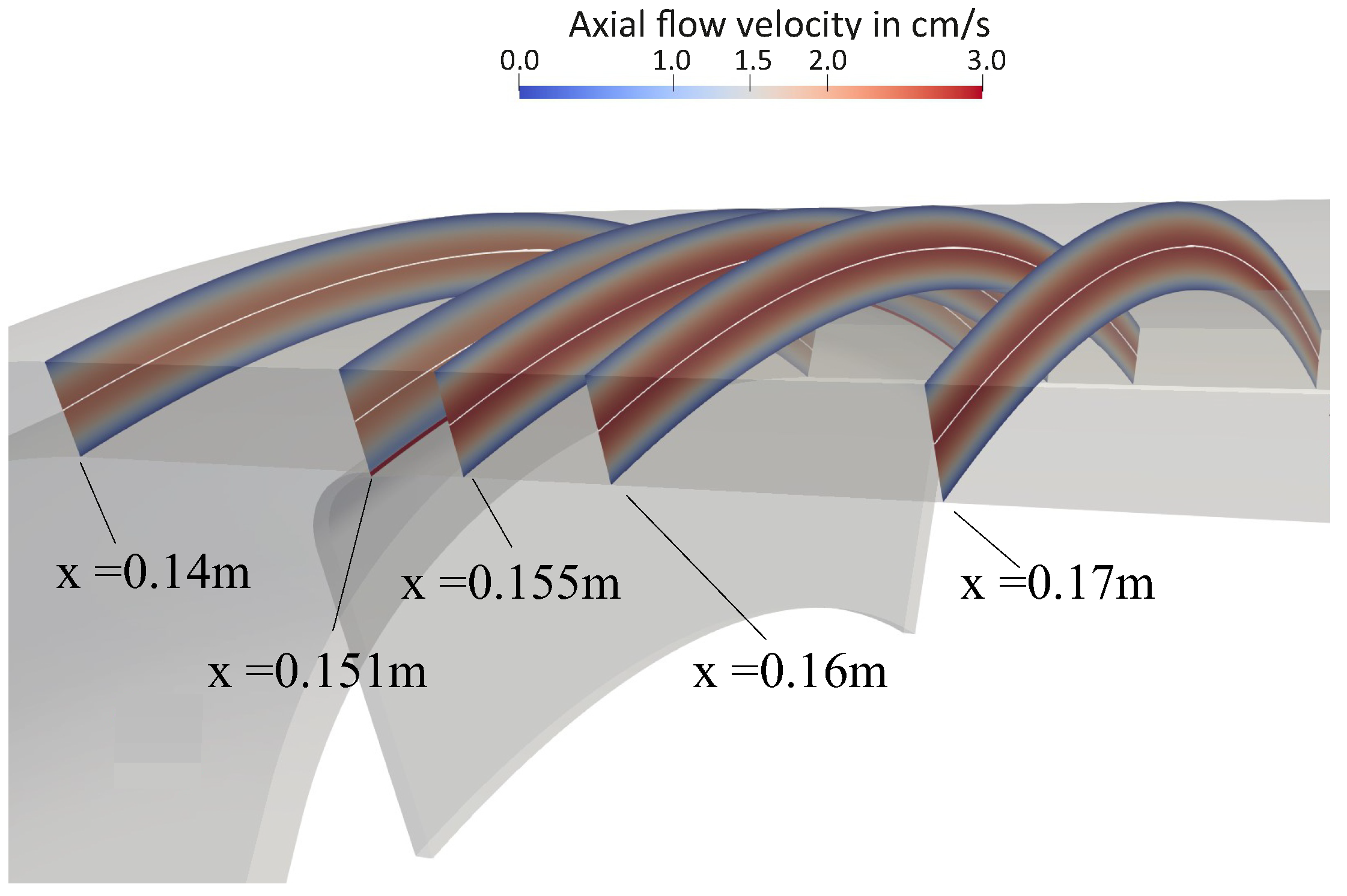
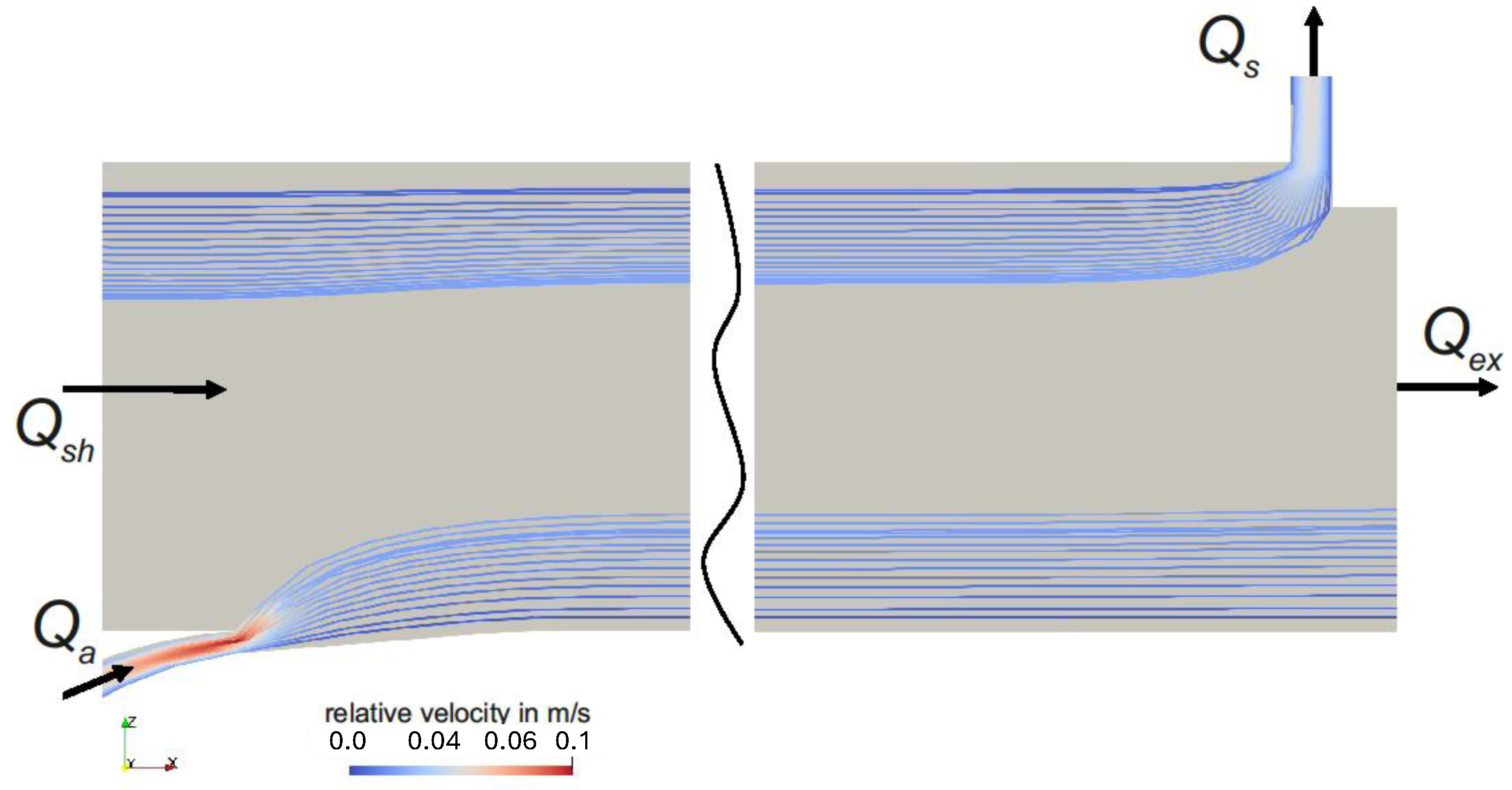
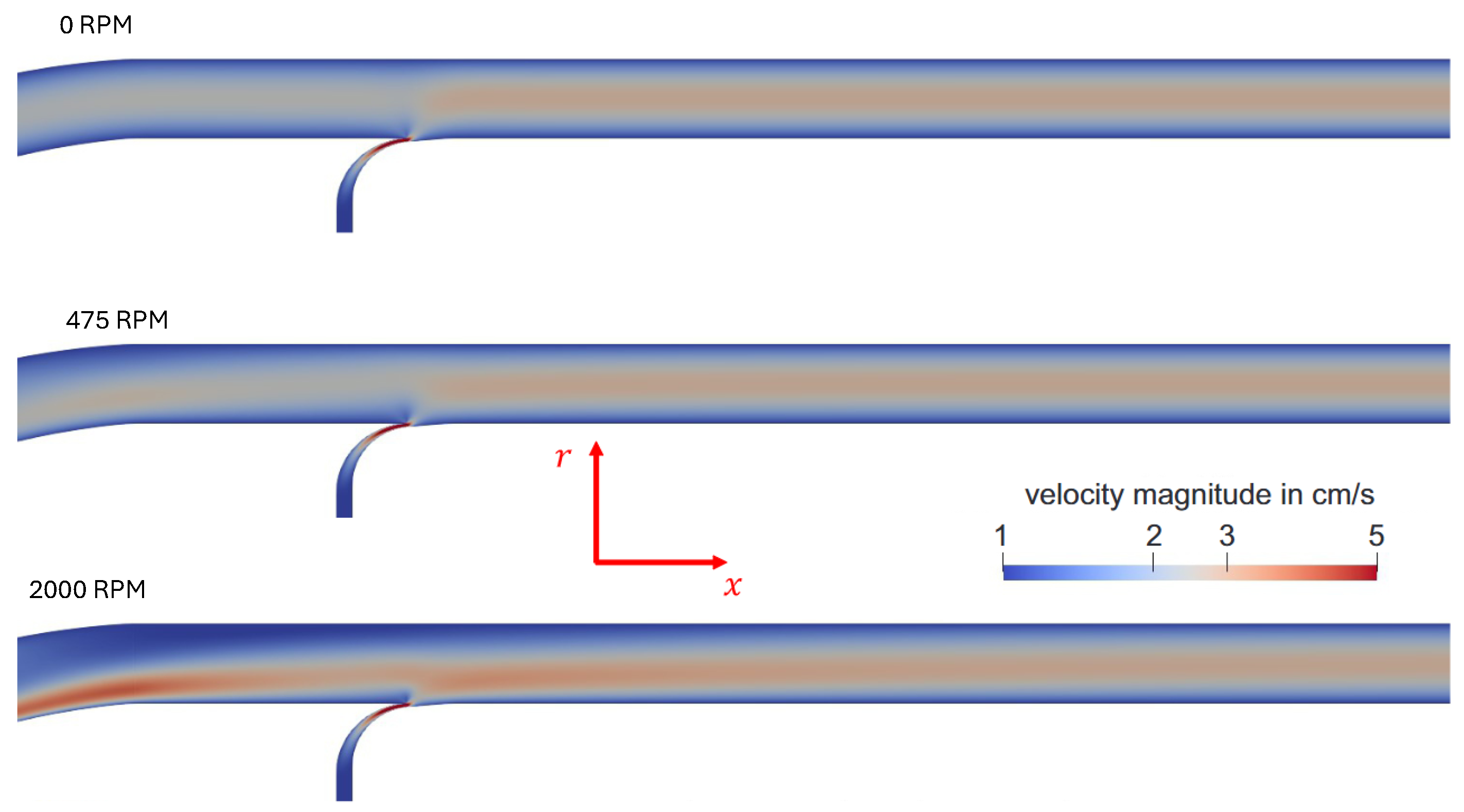
4.1. Flow Behavior Without Rotation

To investigate the radial symmetry of the flow, Figure 3 shows the flow pattern at different positions. Here, x is the absolute position in axial direction, where the inlet of the sheath air is at x = 0 m . For reasons of clarity, the velocities in the axial direction in the highlighted planes are color coded. At the axial coordinate x = 0.14 m , the deflection of the sheath air is completed. The plane at x = 0.151 m is located directly before the aerosol joins the sheath air. It can be observed that the flow profile is symmetrical across the gap width, with no significant deviations in the circumferential direction.
Figure 4 provides a more detailed representation of the axial velocity. On the left, the axial velocity is plotted against the radial coordinate for ϕ = 0 ° . It can be observed that a uniform velocity profile is quickly established. At x = 0.155 m , which is only 4 mm downstream from the point where the aerosol volume flow merges with the sheath air flow, no deviations from the subsequent flow profiles are evident. The right side of Figure 4 further investigates this by showing the velocity profiles along the center of the gap, enabling a more precise analysis of the circumferential direction (indicated by the white lines in Figure 3). In this region, the values across the circumferential direction show only slight variations, which can be attributed to the eight inlet flows. Moreover, it is observed that this small difference (less than ± 0.5 % ) diminishes further as the axial coordinate x increases. This observation suggests that there are no significant variations in the flow profile along the circumferential direction. Therefore, it can be assumed that the flow profile in the middle plane ( ϕ = 0 ° ) is representative of the overall flow profile within the CDMA. As a result, only the flow profile in this middle plane is presented and utilized in the subsequent analyses and calculations.
Figure 5 shows the streamlines at 0 RPM for this middle plane at ϕ = 0 ° . As the streamlines in this region are exceptionally smooth, showing no indication of vortex formation or interaction with the surrounding airflow, it can be reasonably assumed that neither cross-mixing nor backflow occurs. However, a significant expansion of the aerosol flow is observed, which can be attributed to two primary factors: First, the CDMA has been designed so that, for β = 0.1 , the inlet cross section and the sheath air cross section correspond to the respective flow rates. At β = 0.2 , the higher aerosol flow Q a needs to occupy more space. Second, the non-slip boundary condition at the wall leads to a reduction in the flow velocity near the walls, and therefore, the streamlines must expand towards the center of the gap.

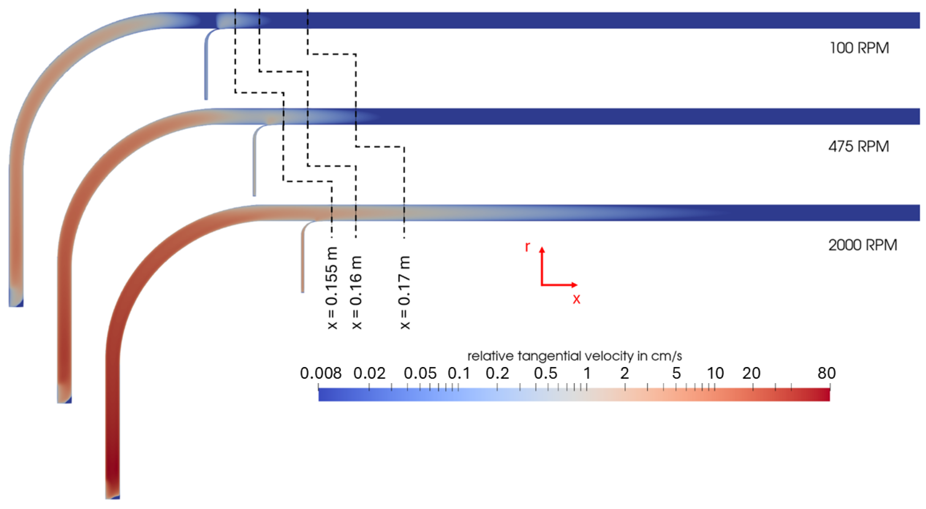
4.2. Flow Behavior with Rotation

Figure 6 shows the angular distribution of the axial velocity at different positions in axial direction analogous to Figure 4, but now for different rotational velocities. It can be observed that the flow profile shifts inward, particularly at higher speeds, and exhibits a higher maximum velocity. However, this effect diminishes as the x-coordinate increases. The velocity profile in the circumferential direction at the center of the classification gap (c.f. Figure 6, right) is also less uniform compared to the non-rotating case, with deviations of up to ± 5 % . Despite these deviations, the profile tends to converge towards the ideal profile as the flow progresses. While these deviations are noteworthy, it is important to consider that they primarily occur at very high speeds and that the deviations decrease with increasing x-coordinates. Therefore, when analyzing the flow with rotation, here only the middle plane ( ϕ = 0 ° ) will be considered moving forward.
In Figure 7, axial velocity fields of the cases for 0, 475, and 2000 RPM are compared. It can be observed that for increasing rotational speed, the velocity profile increasingly shifts toward the inner wall of the transfer domain and shows higher peak velocities. Downstream in the axial direction, the effective cross-section widens up to the geometrically available cross-section. This results in a more symmetric profile for the axial velocity.
Upon examining the inlet region, it becomes evident that a significantly higher flow velocity is observed here compared to other regions. However, even in this region, the flow characteristics do not indicate the formation of vortices. It is important to note that this conclusion is based on the current simulation model, which lacks the capability to accurately capture such detailed flow phenomena. To investigate vortex formation and accurately resolve the flow field, more advanced simulation techniques such as Large Eddy Simulation (LES) or Direct Numerical Simulation (DNS) would be required. These methods would enable a more precise representation of the flow dynamics, particularly in the critical areas where vortices may form.
In general, the presence of turbulence would lead to cross-mixing between adjacent streamlines, resulting in a broadening of the flow profile. This broadening would cause a significant deterioration in the resolution of the transfer function, as it would blur the distinctions between different particle size classes. Thus, turbulence is considered prohibitive in this context, as it would compromise the accuracy and performance of the system.
Figure 8 illustrates the relative tangential velocity, i.e., the deviation of the tangential velocity from solid body rotation. It is evident that the air is unable to immediately match the rotational speed, particularly when there is a flow in the radial direction. This effect can be attributed to the low viscosity of the fluid and the relatively large gap width, which hinder the immediate transmission of rotational speed. As the flow velocity increases, the difference between the rotational and axial velocities also becomes more pronounced, but this disparity is eventually compensated over time.
This phenomenon also highlights that the velocity profile initially stabilizes near the wall before propagating inward. However, since particles are introduced near the wall, where the flow stabilizes relatively quickly (c.f. Figure 7 and Figure 8), the influence of these variations on the particle trajectories is somewhat minimized.
Therefore, the impact of the actual flow field on the transfer function will be explored in more detail in the subsequent chapter, where the relationship between the flow dynamics and particle behavior is examined comprehensively.

5. Transfer Function of the CDMA

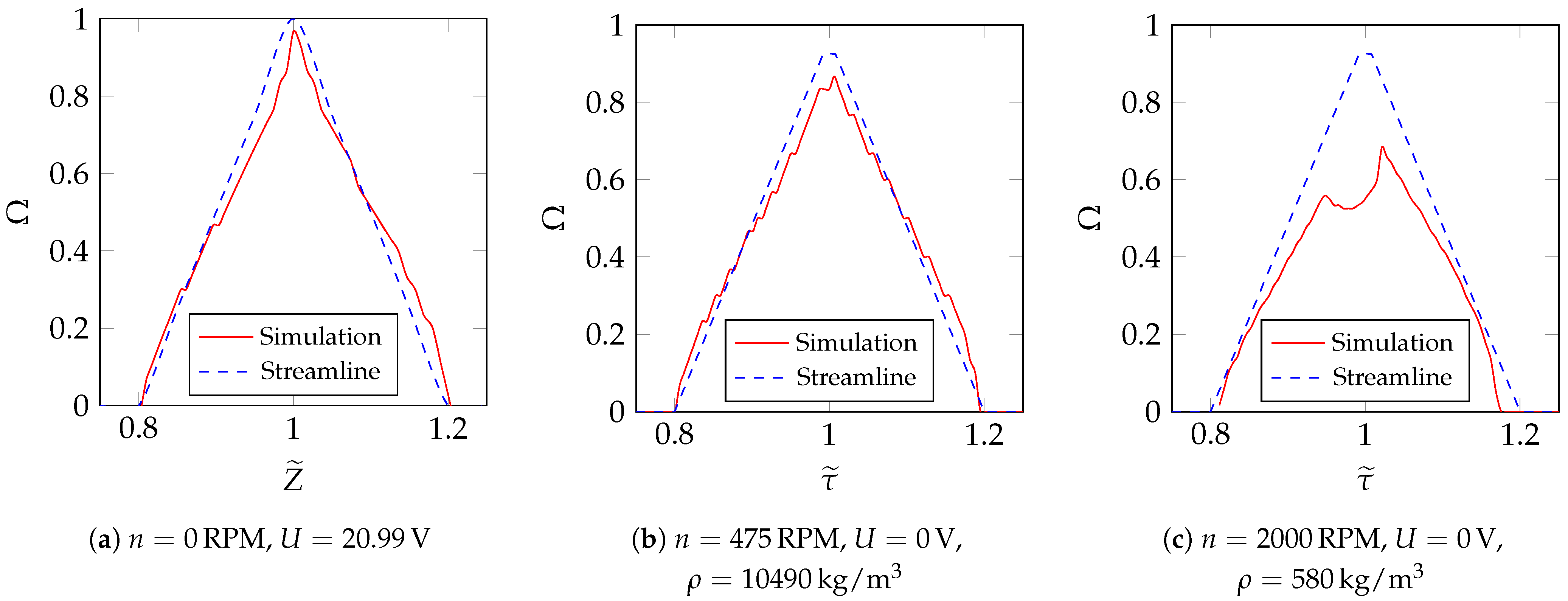
5.1. Transfer Function Based on CFD Simulations

To investigate the influence of the flow profile on the classification, the transfer function was derived directly from CFD data. The determination of a transfer function for specific CDMA operating parameters (at fixed voltage and velocity) is a stepwise process. For each considered particle size, multiple trajectories are calculated while changing the radial particle starting point in the inlet cross section. For singly charged, spherical particles, the transfer probability for one particle size is then given by the number of successfully traversed particles N sampled divided by the total number of simulated particles N tot :
Ω ( d p ) = N sampled N tot
The particle size can then be converted into the mobility Z, particle relaxation time τ or their normalized values ( Z ˜ , τ ˜ ), respectively.
A particle trajectory is calculated using CFD data of the flow simulations. For calculating trajectories, the travelled distance in the radial and axial direction is determined for every calculated time step. The developed algorithm obtains the velocity data of the current particle location. Besides flow velocity data, additional forces are considered to act on the particle in the radial direction. The resulting radial velocity component is calculated using the fluid velocity component in the radial direction, particle size and CDMA operating parameters (c.f. Equation (2)) while neglecting the diffusion and inertia of the particle.
Figure 9 shows trajectories of successfully sampled particles (green) and deposited ones. It is obvious that the resolution of the simulation depends on the number of trajectories, the duration of the virtual time steps and the number of particle sizes investigated. However, these quantities increase only with high computational costs; thus, a compromise must be made.

5.2. Ideal Transfer Function Based on Streamline Approach

To compare the simulated results with theoretical values, we use an ideal transfer function. The ideal two-dimensional transfer function was derived from streamline functions assuming ideal flow profiles and neglecting diffusion. Details for derivation are given in [15].
Ω = 1 2 β ( 1 + A ) · [ | 1 β + κ 2 κ 2 1 · A + Z ˜ τ ˜ · 1 + β 2 h ˜ · A | + | 1 β κ 2 + β κ 2 κ 2 1 · A + Z ˜ τ ˜ · 1 + β 2 h ˜ · A | + | 1 + β β + κ 2 κ 2 1 · A + Z ˜ τ ˜ · 1 + β 2 h ˜ · A | | 1 κ 2 + β κ 2 κ 2 1 · A + Z ˜ τ ˜ · 1 + β 2 h ˜ · A | ]
β is the ratio of aerosol volume flow Q a to sheath air volume flow Q s h , h ˜ is the ratio of the gap width to the mean radius, κ is the ratio of the inner radius r i to the outer radius r o and A is a substitution to facilitate reading.
h ˜ = 2 · r o r i r o + r i
κ = r i r o = 1 h ˜ / 2 1 + h ˜ / 2
A = exp τ ˜ · 2 h ˜ 1 + β 1
This results in a two-dimensional transfer function, as displayed in Figure 10.

5.3. Comparison of Transfer Functions

In the following, we intend to compare the idealized transfer function based on the streamline approach (cf. Section 5.2) with the particle trajectory simulations based on CFD simulations (cf. Section 5.1). However, a quantitative comparison of 2D functions is difficult to visualize. Moreover, the computational effort for determining the 2D transfer function from the particle trajectory simulations would be immense. Therefore, we will compare the transfer functions for τ ˜ = 0 and Z ˜ = 0 (red, dashed lines, cf. Figure 10) in Figure 11 and the transfer function for spherical particles (red solid line, c.f. Figure 10) in Figure 12.
The operational parameters for determining the transfer functions for τ ˜ = 0 and Z ˜ = 0 as illustrated in Figure 11 were selected so that τ ˜ = 1 or Z ˜ = 1 results for a particle size of 100 nm . In order to test for different centrifugal conditions, two different densities were chosen in Figure 11b and Figure 11c, respectively. It is evident that the resolution of the simulation results is limited because of the restricted number of calculated particle trajectories per particle size. An investigation of the pure electrical mode (see Figure 11a) reveals a high degree of agreement between the transfer functions. The minor discrepancies can be attributed to the flow field and the limited resolution. Figure 11b,c illustrate the transfer functions at different speeds in purely rotational mode. The transfer functions exhibit a high degree of agreement for the case of 475 RPM (see Figure 11b). The simulated transfer function is slightly lower, indicating a slightly reduced probability of classification around τ ˜ = 0 . As the speed increases (cf. Figure 11c), the relative position of the transfer function remains consistent, while the height of the transfer function is reduced significantly. This can be attributed to the increasing distortion of the flow field especially at the edges of the aerosol inlet and sample outlet. It is likely that small flow deviations at the edges of the inlet and outlet lead to increasing losses so that especially the tip of the transfer function, where over the whole gap all particles should be sampled, will be decreased significantly in height.
To extend the investigation of the transfer functions, the combination of applying both voltage and rotational velocity is examined, too. To simplify the two-dimensional transfer function to a one-dimensional transfer function, perfectly spherical particles carrying one elementary charge are considered (c.f. red solid line in Figure 10 as an example). In this case, small particles with high electrical mobility and low mass and larger particles with lower mobility and high mass are classified simultaneously, resulting in two peaks of the transfer function, as shown in Figure 12.
Varying the operating parameters results in a shift of the two peaks until they merge and eventually diminish. The simulated transfer functions are again very close to the ideal transfer functions but show a slightly smaller height at higher centrifugal forces.
This indicates that the transfer functions derived from the simulation are accurately represented by the theoretical streamline calculation. Furthermore, the results demonstrate that the flow profile within the CDMA has no significant impact on the transfer behavior as long as it stays laminar. At higher speeds, a small distortion of the transfer function occurs when the circumferential speed is not yet fully developed at the inlet of the classification gap. The absence of a shift in the transfer function serves to substantiate the assertions outlined in Section 4.2, which posits that the flow profile exerts no essential influence in this particular context.
It should be pointed out that the boundary condition at the aerosol inlet has a much more severe influence on the transfer function: A previous study [15] showed that the assumption of a constant particle concentration and a laminar flow profile at the aerosol inlet may lead to significantly different transfer functions if compared to the assumption of a constant particle flux density at the aerosol inlet as typically assumed and as applied in this study.

6. Measurement of Transfer Functions

In order to validate the theory and the experimental CDMA prototype, the real transfer function has been investigated experimentally.

6.1. Theory

As shown in Ruther et al. [14], a tandem setup comprising a DMA and a CDMA is employed to determine the transfer functions Ω (c.f. Figure 13). Following the assumption of a broad distribution of the test aerosol, the ratio of the number concentrations ( n 1 and n 2 before and after the CDMA classification) can be described as follows [20]:
n 2 / n 1 = + Ω 1 Z ˜ · Ω 2 Z ˜ d Z ˜ + Ω 1 Z ˜ d Z ˜
The transfer functions in general are well described by Gaussian functions [15]. Therefore, the transfer function Ω 1 of the pre-classifying DMA and the transfer function Ω 2 of the CDMA at zero rotation can be described using the parameters of the Gaussian function Ω 1 , max , Ω 2 , max , μ ˜ 1 , Z ˜ , μ ˜ 2 , σ 1 , Z ˜ , σ 2 as follows:
Ω 1 = Ω 1 , max · exp ( Z ˜ μ ˜ 1 , Z ˜ ) 2 σ 1 , Z ˜ 2 ; Ω 2 = Ω 2 , max · exp ( Z ˜ μ ˜ 2 ) 2 σ 2 2
Inserting Equation (14) in Equation (13) leads to [14]:
n 2 / n 1 = Ω 1 , max · Ω 2 , max · 1 σ 1 , Z ˜ 2 + σ 2 2 · exp ( μ ˜ 2 μ ˜ 1 , Z ˜ ) 2 σ 1 , Z ˜ 2 + σ 2 2
This means that measuring the ratio n 2 / n 1 for a fixed voltage applied to the upstream DMA (i.e., μ 1 , Z ˜ fixed) while varying the voltage of the CDMA (i.e., varying the μ ˜ 2 ), makes it possible to determine the transfer function by simply fitting a Gaussian function to the measured n 2 / n 1 ( μ ˜ 2 ) , if the transfer function of the pre-classifying DMA is known [14].
The exact approach to determine these parameters with high accuracy is described in Appendix B, so that c Z ˜ and μ ˜ 1 , Z ˜ are determined as follows:
σ 1 , Z ˜ = 0.5732 · β
μ ˜ 1 , Z ˜ = 1.0154
This procedure for determining the transfer function of a DMA-DMA setup can be applied to a DMA-AAC setup (or in this case a DMA-CDMA setup with the CDMA operated at U = 0 V ) as well. In the case of spherical particles, the mobility of the first DMA can be converted into the particle relaxation time.
Defining the transfer functions as follows:
Ω 1 = Ω 1 , max · exp ( τ ˜ μ ˜ 1 , τ ˜ ) 2 σ 1 , τ ˜ 2 ; Ω 2 = Ω 2 , max · exp ( τ ˜ μ ˜ 2 ) 2 σ 2 2
Because of the charge distribution, other particle sizes can pass the pre-classifying DMA as well. Therefore, the particle number is quite different for the considered particle size interval. This must be corrected, as shown in Rüther et al. [14]. The following parameters can then be determined by applying Equation (A1).
σ 1 , τ ˜ = 0.6369 · β
μ ˜ 1 , τ ˜ = 0.99477
These values can be used to calculate the transfer functions for the CDMA corresponding to Equation (15), i.e., replacing σ 1 , Z ˜ and μ 1 , Z ˜ by σ 1 , τ ˜ and μ 1 , τ ˜ , respectively.

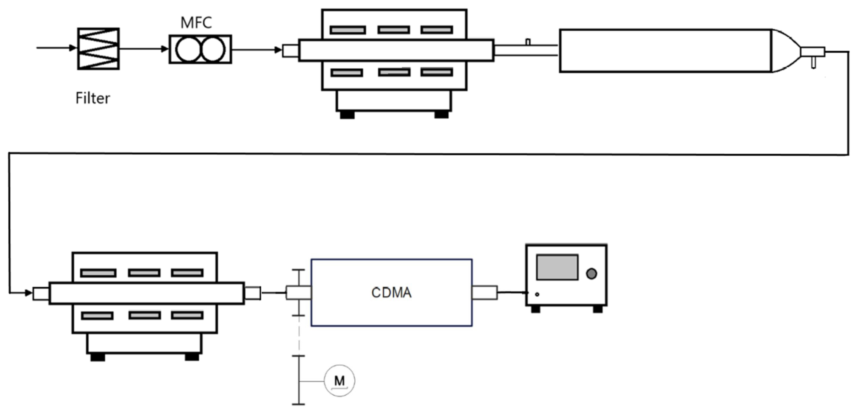
6.2. Production of the Test Aerosol and Measurement Setup

A method for producing an aerosol of a relatively immutable, broad particle size distribution for a large time period was developed using a setup comprising two hot-wall reactors with an agglomeration tube ( V = 10 l ) positioned between them (see Figure 13). An air flow rate of ( 2 l / min ) controlled by a mass flow controller (MFC) is introduced into the setup. Silver is melted and evaporated at a temperature of 1150   ° C within the upstream hot-wall reactor. Upon cooling towards the exit of the first furnace, the vapor becomes supersaturated, resulting in the immediate formation of silver particles. Subsequently, larger agglomerates are formed in the agglomeration tube, which are ultimately sintered into spherical particles in the second hot-wall reactor at 750   ° C .
Subsequently, the spherical particles are pre-classified in a DMA, which is set to a specific mobility value. The valves V 1 and V 2 allow to bypass the CDMA completely, allowing to directly determine the number concentration n 1 by the CPC. Alternatively, by closing the bypass route, the aerosol will be classified by the CDMA. In this case, the CDMA was programmed to run sweeps for the voltage or the rotational velocity, respectively. Consequently, the CPC will determine the number concentration n 2 as a function of the operating parameter n 2 = f ( U , ω ) .

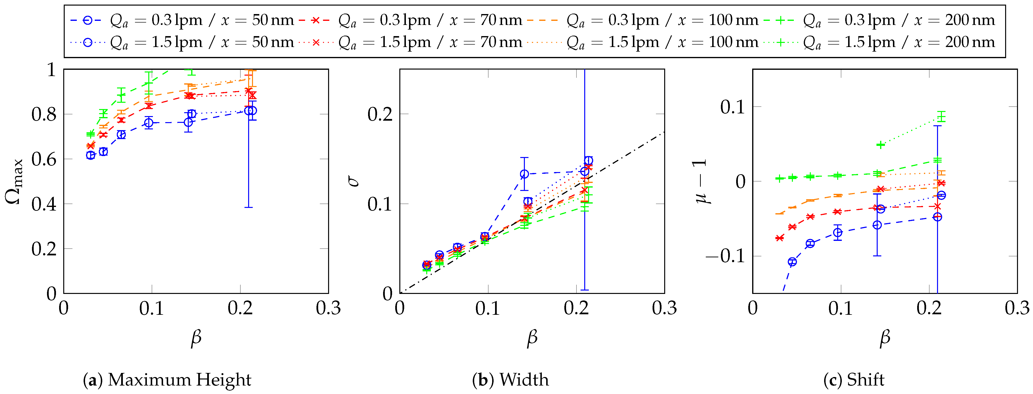
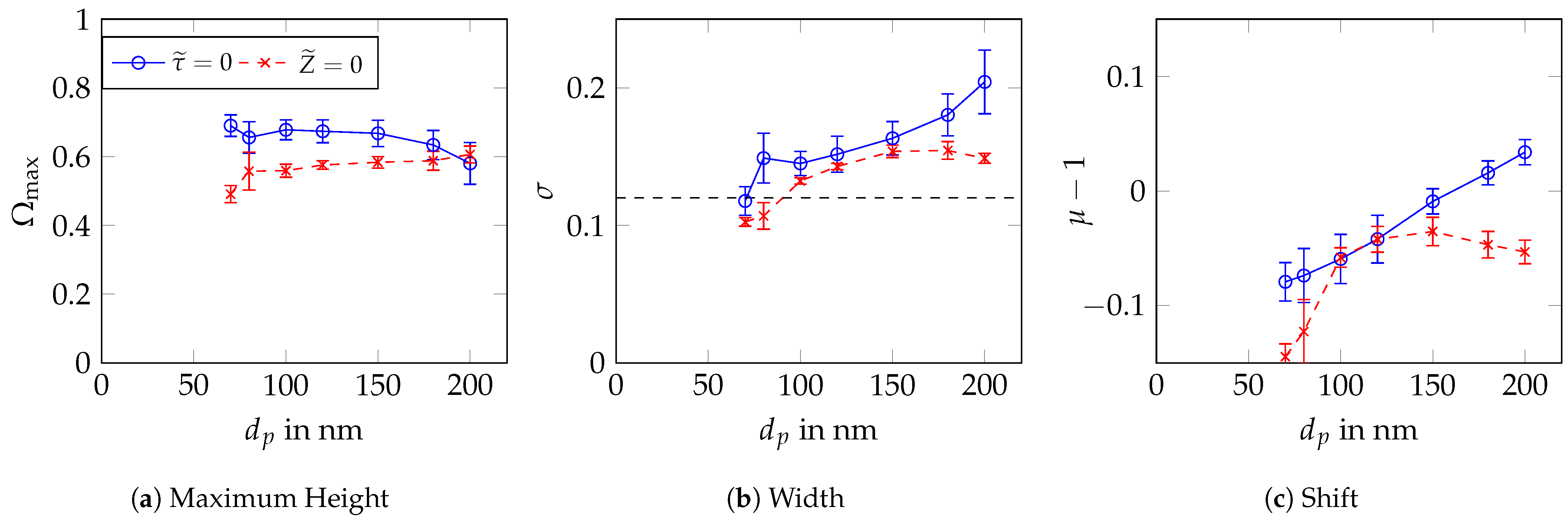
6.3. Experimental Determination of the CDMA Transfer Function for τ ˜ = 0 and Z ˜ = 0 at Different β -Values

Transfer functions of the CDMA prototype have been determined as described in the previous section. However, these transfer functions are not only affected by the deterministic particle trajectories in the classification gap. In the case of the CDMA prototype geometry where the gap width is quite small, diffusion strongly influences the transfer function. This leads to a broader transfer function with reduced height. However, the change in the transfer functions can be theoretically predicted pretty well [15]. Additionally, Rüther et al. [14] demonstrated that in the CDMA prototype, increased losses occur in the sample outlet due to still-existing electric and centrifugal fields. Nevertheless, as shown in Rüther et al. [14], such losses can be predicted by particle trajectory simulation based on the respective electrical and centrifugal fields. Such predicted losses can be used to correct the measured transfer functions accordingly. In the following, all presented parameters of the transfer functions have been adapted after performing corresponding corrections to the measured transfer functions [14]. Therefore, the presented results should describe the transfer function of the deterministic classification process in the CDMA gap.
Figure 14 illustrates the parameters of this CDMA transfer function over a range of operational parameters in ‘DMA mode’, i.e., for τ ˜ = 0 . When considering the height of the transfer function Ω max in Figure 14a, it is noticeable that there are obviously additional losses not covered by the above-mentioned simulations. Moreover, these additional losses in the aerosol inlet and outlet are particularly present in the case of reduced aerosol volume rates due to increased residence times. It is noteworthy that values exceeding 1 were observed in a few cases, which can be attributed to potential measurement errors or inaccuracies in the determination of the transfer function of the pre-classifying DMA.
However, the width of the transfer function is nearly identical to the calculated ideal width (cf. Figure 14b). This indicates, that the broadening according to diffusion is well captured by the simulation so that the width of the corrected transfer function agrees very well with the expectations. Only the measurement series for 0.3 l / min exhibits a slight elevation for 200 nm particles, which most likely can be attributed to measurement errors. This is due to poor statistics because only a very small number of particles were counted at 200 nm , as this was at the edge of the particle size distribution of the test aerosol.
The shift of the transfer function (Figure 14c) is small and comparable to the results obtained for standard DMA instruments, which are presented in Figure A2, Figure A3, Figure A4, Figure A5, Figure A6 and Figure A7 in Appendix B.
The transfer functions for Z ˜ = 0 , i.e., operating the CDMA in AAC mode, are illustrated in Figure 15. It is important to note that for β < 0.1 , there is no measurable transfer function. This is due to massive particle losses occurring at the outlet due to the prevailing centrifugal forces. Thus, each measurement series comprises only two data points [14].
Figure 15a illustrates the maximum height of the transfer functions. Despite the corrections, the transfer function remains dependent on the particle size and the prevailing flow conditions. This finding is particularly relevant in the context of rotational operation, because even small imperfections, such as deviations in production, a non-concentric alignment of both cylinders, and similar factors have a greater impact on the flow field, generating this dependency. The measurement was conducted over the entire CDMA (including transport to and from the measurement gap), thus precluding the possibility of correcting all undetermined losses. However, no direct correlation could be established between the corrected measurement values and further diffusion in the inlet and outlet. A number of other loss mechanisms occur here that cannot simply be separated. Thus, no equivalent loss length for diffusion, as would be present when flowing through a pipe, could be determined.
Figure 15b illustrates the width of the transfer function. The measured values displayed do not exhibit a correlation with the beta values as the range of variation is too big. This can be attributed to the inaccuracies and the considerable losses of the CDMA system. In comparison to τ ˜ = 0 , a non-negligible shift in the transfer function (c.f. Figure 15c) is also present. This indicates a dependency on particle size, volume flows or rotational speed.

6.4. Experimental Determination of the Transfer Function for τ ˜ = 0 and Z ˜ = 0 at β = 0.2

In this section, we will focus on the targeted operating conditions of the CDMA ( Q a = 0.3 l / min at β = 0.2 ). As part of this investigation, the transfer functions for particles of varying sizes are measured once more under these conditions. The resulting data are presented in Figure 16.
After the correction of simulated modification by diffusion in the measurement gap and simulated losses due to electrical and centrifugal forces in the outlet, it can be observed that the heights of the transfer functions (see Figure 16a) are only weakly depending on particle size in the examined size range from 50 nm to 200 nm . Even for operation in ‘DMA mode’ or ‘AAC mode’ the heights of the transfer functions are in a similar range. It is notable that the widths of the transfer functions exhibit a slight upward deviation for larger particles, which again can be attributed to the poor statistics due to a relatively low particle number of particles exceeding 150 nm .
If all applied corrections as outlined above would cover all non-idealities, the resulting height of the transfer functions shown in Figure 16a should be close to 1 for all particle sizes. However, if we determine an average value from all measured height values, we obtain a height reduction factor, η HeightRed = 0.61 . In fact, this η HeightRed accounts for all additional losses, e.g., diffusional losses in the inlet and outlet tubing, losses due to centrifugal forces in the inlet section, etc.
Thus, the real transfer function can be well estimated by correcting the theoretical transfer function (c.f. Section 5) with simulated modifications by diffusion as well as simulated losses in the outlet due to electrical and centrifugal forces as outlined above and subsequent scaling with η HeightRed . Since the width of the transfer function does not exhibit significant variations, particularly not in a systematic manner, the width of the transfer function is adopted according to the mean width, as shown in Figure 16b. Additionally, a shift correction factor, ϵ Shift = 0.051 , is introduced to align the theoretical transfer function with the experimentally measured one.
By assuming that these corrections are applicable not only to the transfer functions at Z ˜ = 0 and τ ˜ = 0 but also to the entire two-dimensional transfer function, a generalized description of the real transfer function for any given operating condition is obtained.

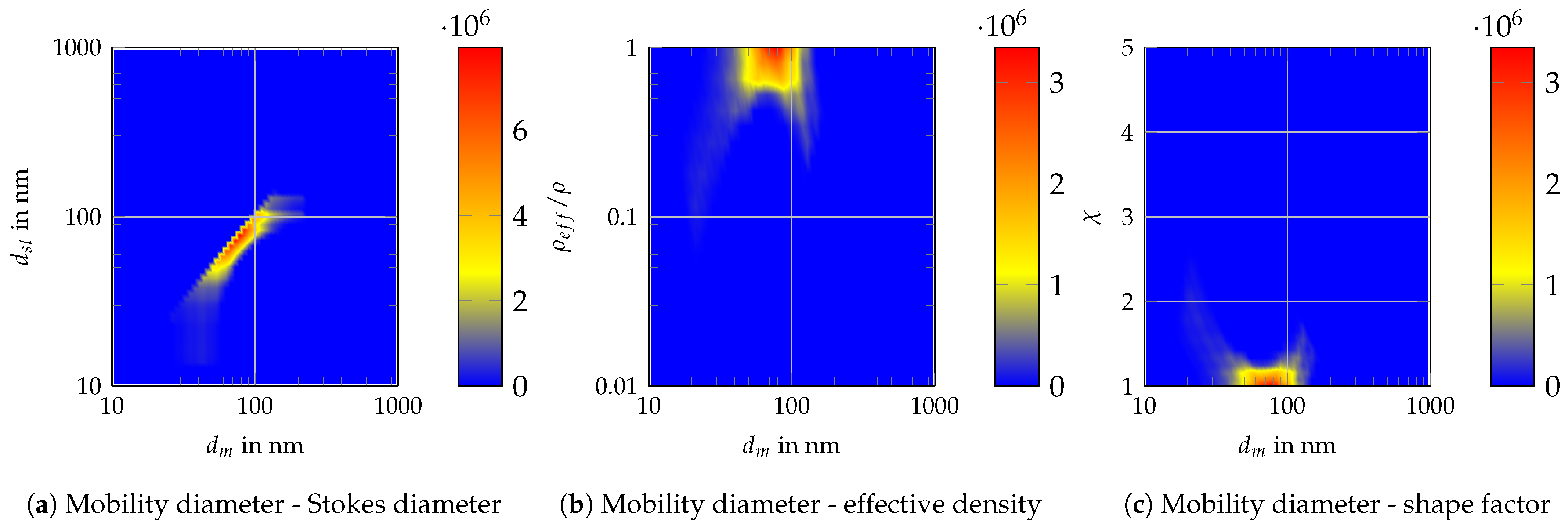
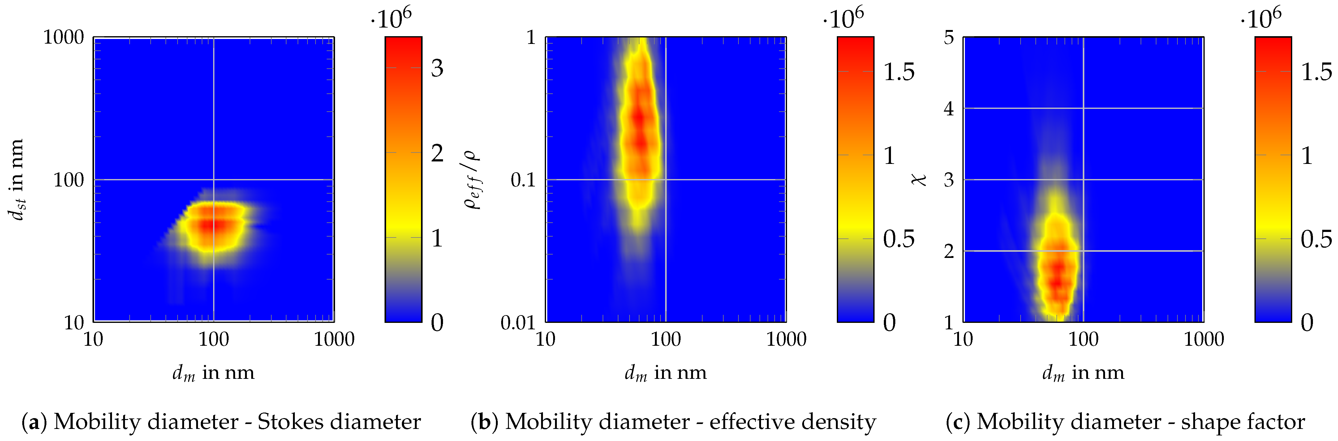
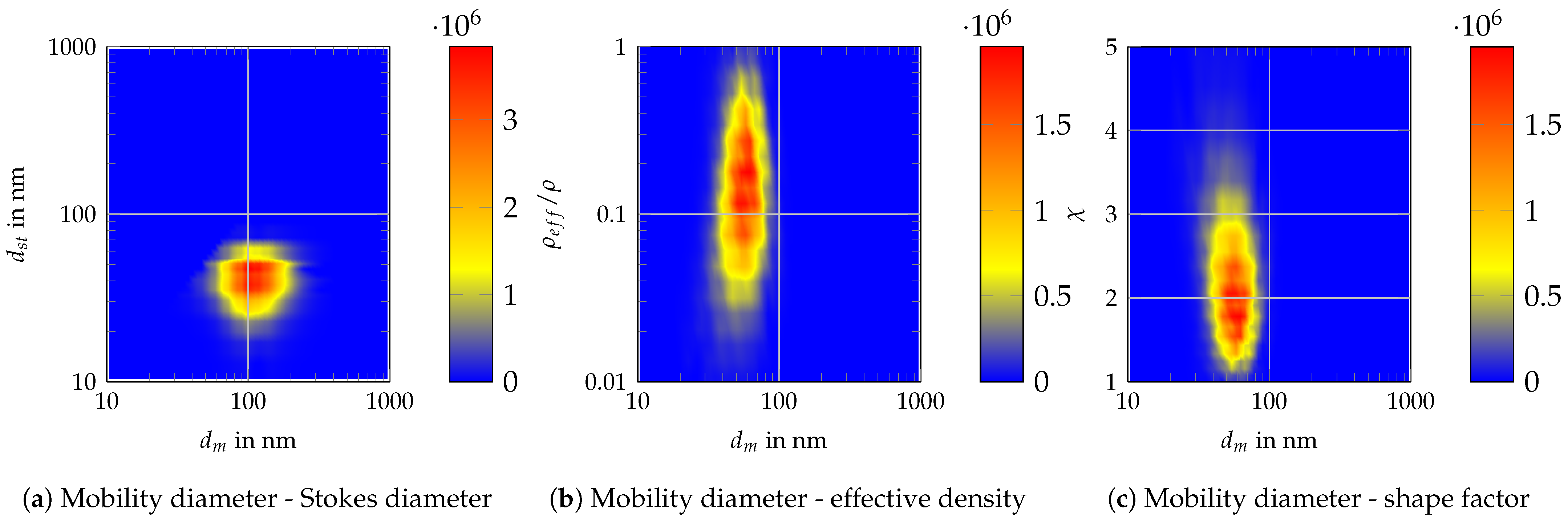
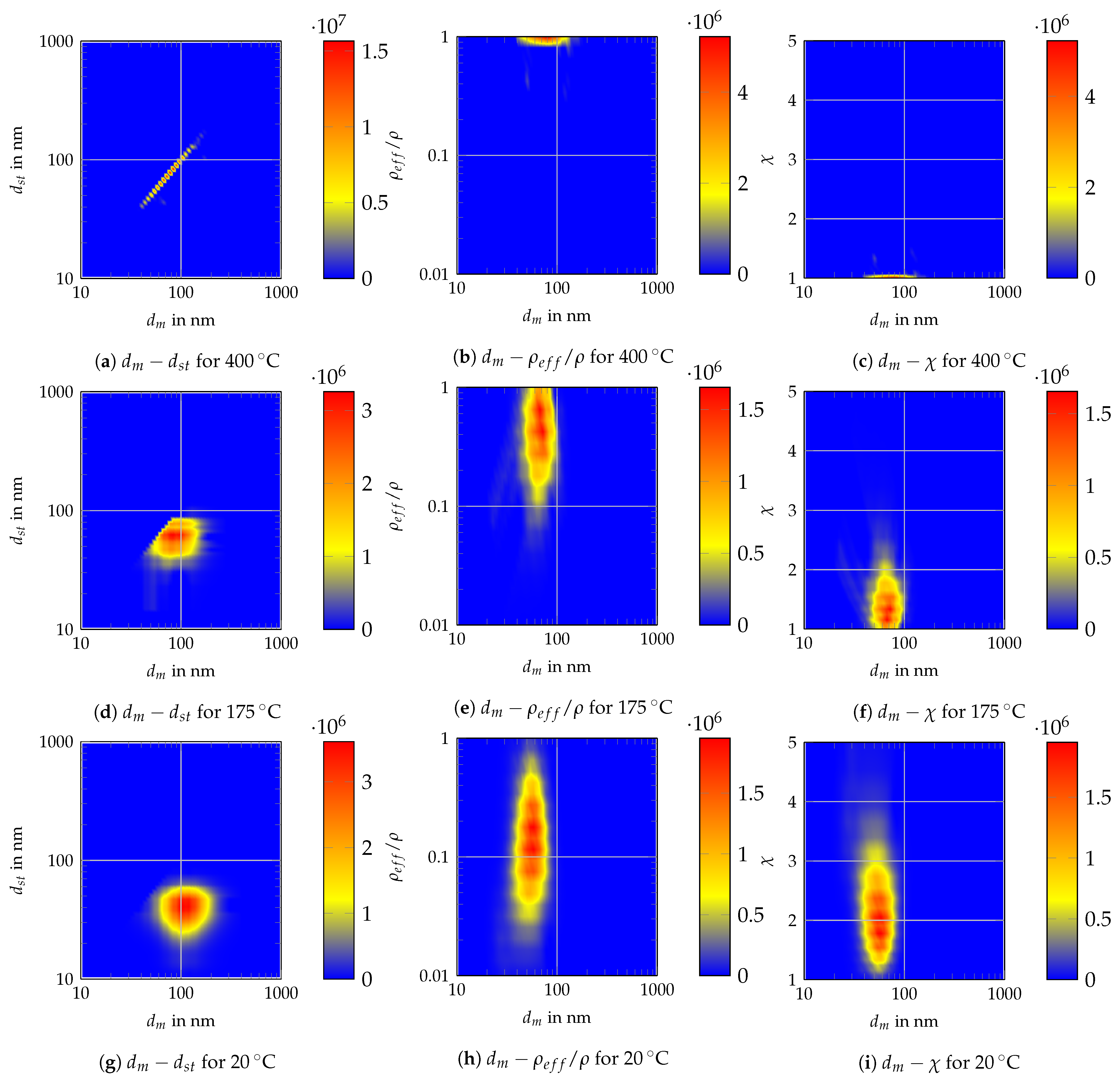
7. Measurement Results and Analysis of Two-Dimensional Size Distributions for Different Sintering Stages of Silver Nanoparticles

The previous section provided a brief overview of the measurement process for determining the transfer function of the CDMA. Unlike the ideal transfer function, the measured transfer function inherently accounts for all real-world imperfections and deviations. To accurately model the system, the ideal transfer function is adjusted based on these measured values (as explained in Section 6.4). This 2D transfer function is then used to calculate the kernel matrix K ̲ i , j , k , l , which must be known in order to calculate the expected measured sample number concentrations for given operating conditions Δ N ( U i , ω j ) for a given 2D particle size density distribution q ( d m , k , d S t , l ) with respect to mobility diameter d m and Stokes diameter d S t :
Δ N ( U i , ω j ) N tot = k l K ̲ i , j , k , l · q k , l · Δ log ( d m , k ) · Δ log ( d S t , l )
Details on how this kernel matrix can be derived for a given 2D transfer function are given in [16].
In order to determine a 2D size distribution from measured number concentrations at the CDMA sample outlet requires an inversion of a so-called ill-posed problem. As outlined in the introduction, there are many different approaches to solving such inversion problems. As described in detail by Rüther et al. [16], the POCS (Projection onto Convex Sets) algorithm which is well established e.g., in the field of image reconstruction, was applied to a particle characterization problem for the first time. It is an iterative algorithm that allows to consider an arbitrary number of conditions, e.g., Equation (21), marginal distributions, which can be determined independently by operation of the CDMA in ‘DMA mode’ and ‘AAC mode’, respectively, and the normalization of density distribution or non-negativity of density distribution. This algorithm proved to be excellently suited to efficiently and accurately solve this inversion problem.

7.1. Production of the Aerosol and Measurement Setup for Two-Dimensional Distributions

The first measurements of a two-dimensional particle size distribution are carried out using the test aerosol setup shown in Section 6.2 but with no pre-classifying DMA. This setup is shown in Figure 17. In this study, agglomerates at different sintering stages shall be produced by controlling the temperature of the second furnace intended for controlled sintering. Here, temperatures of 20   ° C , 60   ° C , 100   ° C , 175   ° C , 250   ° C , and 400   ° C are used.

7.2. Derivation of Further Properties

From the two-dimensional distribution of the mobility and Stokes diameter, it is possible to derive other quantities characterizing the particle shape like the aerodynamic d a e and volume d v equivalent diameters, the effective density ρ e f f or the shape factor χ [21].
d a e = d s t · ρ / ρ 0
d v = ( d s t 2 · d m ) 1 / 3
ρ e f f / ρ = ( d v / d m ) 3
χ = d m / d v
Since a sphere experiences a smaller drag force than any other particle of the same volume, the following relations are valid:
ρ ρ e f f ; χ 1 ; d m d v d S t

7.3. Measurement Results

Figure 18 shows the two-dimensional distributions of the aforementioned quantities at different sintering temperatures. The measurement comprises 29 voltages, which are logarithmically distributed between 0 and 250 V, and 14 speeds, which are logarithmically distributed between 0 RPM and 1500 RPM . This results in a total measurement time of about 12 h. We are aware that such a measurement time is not acceptable for many applications. However, we expect to reduce this measurement time by a factor 10–20 by continuously scanning the voltage instead of increasing it stepwise. Furthermore, after the marginal distributions are measured right at the beginning by running scans in ‘DMA mode’ and ‘AAC mode’, respectively, an intelligent, automatic determination of the relevant range for U and ω will further reduce the required measuring time.
At high sintering temperatures (for example, 400 ° C, as shown in Figure 18), the agglomerates are supposed to be completely sintered forming almost perfect spherical particles. This can be clearly seen from all representations of the measured 2D distributions: the relative effective density ρ e f f / ρ and shape factor χ for all particles are close to 1 and, therefore, the ρ e f f / ρ d m -distribution and the χ d m -distribution are becoming more or less 1D-distributions of d m , with the other value being constant. The d s t / d m -distribution shows a bi-sectional distribution since for spherical particles, d m = d s t .
For lower sintering temperatures, more irregularly shaped agglomerates are produced, and therefore, the relative effective density becomes lower than 1, and the shape factor becomes larger than 1. Consequently, true 2D distributions can be determined giving detailed information about the size and structure of the agglomerates (c.f. Figure A8, Figure A9 and Figure A10 in the Appendix C for more sintering stages in between). Since the Stokes diameter is always less or equal to the mobility diameter, the corresponding 2D distribution is more skewed towards d m for less sintered agglomerates. It can be clearly seen that for a sintering temperature of 175 ° C, there are still a few almost spherical particles while only agglomerate particles with quite diverse mobility shape factor larger than 1 are present if the second furnace is set to 20 ° C, i.e., no sintering occurs at all.
It is clearly demonstrated that the new measurement technique provides a powerful means to determine valuable information about the size and structural properties of the agglomerates. This can be used to obtain a deeper understanding of aerosol synthesis if applied to corresponding processes. In particular, relevant particle properties can be determined by directly enabling, for example, the optimization of the synthesis conditions for generating particles more efficiently.

8. Conclusions

The proposed methodology for determining two-dimensional property distributions has significant potential for both research and industrial processes. With these additional insights, the behavior of complex particle systems can be more comprehensively understood.
The Centrifugal Differential Mobility Analyzer can measure two-dimensional distributions, e.g., regarding the mobility and Stokes diameter, thus enabling the investigation of the distribution of different other characteristic property values. The new approach has the advantage that the measurement can be performed with one single instrument and be evaluated with an established inversion algorithm. Moreover, avoiding the tandem set-up provides much better statistical significance due to higher particle concentrations at the sample outlet. The functionality of the prototype was validated and then meticulously characterized to identify potentials for further improvements. Even though a number of weaknesses in the first prototype were identified, it is feasible to determine the actual transfer functions with good accuracy, thereby enabling data inversion on this basis. The data inversion is highly robust and yields plausible results [16], which can be converted into further property distributions. In comparison with one-dimensional measurement techniques, the CDMA offers a substantial increase in the amount of information obtained.
As the next step, the design of the CDMA prototype will be comprehensively revised to significantly reduce losses in the inlet and outlet regions, thereby improving measurement accuracy [14]. This optimization can be further enhanced by employing more advanced CFD simulations, particularly including the complete inlet and outlet regions and attached tubings, to resolve all flow non-idealities accurately. Simulating particle trajectories based on these flow simulations should then allow to predict all losses more accurately. Additionally, diffusion can be minimized by increasing the gap width [15], while the flow field within the CDMA can be optimized for higher rotational speeds. Furthermore, the implementation of a scanning mode for the voltage, as applied in SMPS systems, will enable a substantial reduction in the measurement time, thereby rendering the entire measurement process less susceptible to errors, i.e., fluctuations of the aerosol generation process. At that stage, it will become considerably more straightforward to examine other particulate systems and assess the performance of the CDMA across a range of materials and particle sizes. Subsequent investigations should also cover the further validation of results, such as the actual particle sizes and effective density, using electron microscopy images or a comparison with tandem setups, e.g., a DMA-AAC setup. Furthermore, combining the CPC with a Faraday-Cup-electrometer would result in more information and thus in an improvement in the data inversion quality. Additionally, the introduction of sensitivity analyses concerning operating parameters and diffusion effects could contribute to a more comprehensive understanding of the CDMA.
Moreover, the CDMA set-up is not only useful for determining size and shape. If the particle shape of a test aerosol can be considered as known, it is feasible to determine the charge distribution or the Cunningham slip correction, thereby establishing a novel methodology for determining these properties, particularly for non-spherical particles. Since the presented study focuses on the determination of particle shape by including centrifugal forces, it is essential to know the particle material density with a high degree of precision. However, in the case of unknown particle systems, only the aerodynamic diameter can be determined, giving no direct information on the actual particle shape. However, if particle shape is known (e.g., compact, almost spherical), the 2D size-density-distribution could be determined instead. Moreover, integration with additional measurement systems could enable access to a three-dimensional distribution of properties. For instance, it may be feasible to examine the scattered light behavior of particles to integrate mass spectrometry or low-pressure impaction of the sample aerosol.

Author Contributions

Conceptualization, T.N.R. and H.-J.S.; methodology, T.N.R. and H.-J.S.; software, T.N.R., S.G. and C.D.; validation, T.N.R., S.G. and C.D.; formal analysis, T.N.R.; investigation, T.N.R. and H.-J.S.; resources, T.N.R. and H.-J.S.; data curation, T.N.R. and S.G.; writing—original draft preparation, T.N.R.; writing—review and editing, H.-J.S., S.G. and C.D.; visualization, T.N.R. and S.G.; supervision, H.-J.S.; project administration, H.-J.S.; funding acquisition, H.-J.S. All authors have read and agreed to the published version of the manuscript.

Funding

This work was supported by the German Research Foundation under the SPP 20245 MehrDimPart (GZ: SCHM 1429/19-1).

Data Availability Statement

Code availability is given under: https://git.uni-paderborn.de/pvt/cdma, reference number 11577 (CDMA, 2025).

Conflicts of Interest

The authors declare no conflicts of interest.

Abbreviations

The following abbreviations are used in this manuscript:
CDMACentrifugal Differential Mobility Analyzer
DMADifferential Mobility Analyzer
AACAerodynamic Aerosol Classifier
CPCCondensation Particle Counter
lpmStandard liters per minute
RPMRevolutions per minute
MFCMass-flow Controller

Nomenclature

κratio of ri to ro
βratio of Qa to Qsh
χshape factor
ηdynamic viscosityPas
transfer function of classifier
transfer function
ωangular speed ω = 2π · n1/s
ρparticle densitykg/m3
ρ0assumed reference density of 1000 kg/m3kg/m3
ρeffeffective densitykg/m3
σstandard deviation of Gaussian shaped transfer function
σwidth of the transfer function
τparticle relaxation times
τ* nominal particle relaxation times
K ̲ Kernel matrix
μ ˜ 2 , μ ˜ 1 fit parameters for the shift of a Gaussian function
τ ˜ normalized particle relaxation time
h ˜ ratio of the gap width to the mean radius
Z ˜ normalized particle mobility
accentrifugal accelerationm/s2
CuCunningham slip correction factor
dmmobility equivalent diameterm
dvvolume equivalent diameterm
daeaerodynamic equivalent diameterm
dPdiameter of a spherical particlem
dststokes equivalent diameterm
Eelectric fieldV/m
Llength of the CDMA classification gapm
mPparticle masskg
nnumber of particle charges
Ntottotal number of simulated streamlines#
Ntraversednumber of successfully traversed streamlines#
qparticle density distribution
Qaaerosol volume flowm3/s
QPparticle chargeAs
Qssample volume flowm3/s
Qexexcess air volume flowm3/s
Qshsheath air volume flowm3/s
riinner radiusm
roouter radiusm
raeouter radius of the aerosol air streamlinesm
rsinner radius of the sampling air streamlinesm
UvoltageV
wDrparticle drift velocitym/s
xlength coordinate in axial directionm
Z* nominal particle mobilitym2/(Vs)
Zpparticle mobilitym2/(Vs)

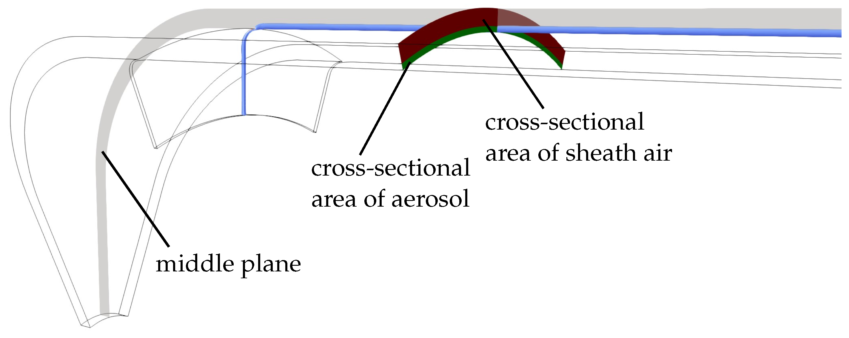
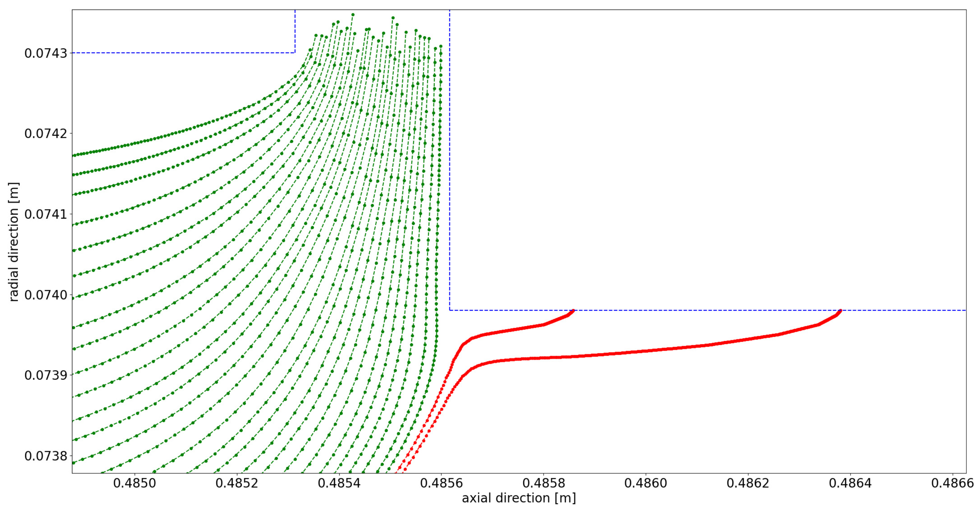
Appendix A. Further Illustration of the CFD Simulation

Figure A1. Schematic drawing of the flow sections and the middle plane.
Powders 04 00011 g0a1

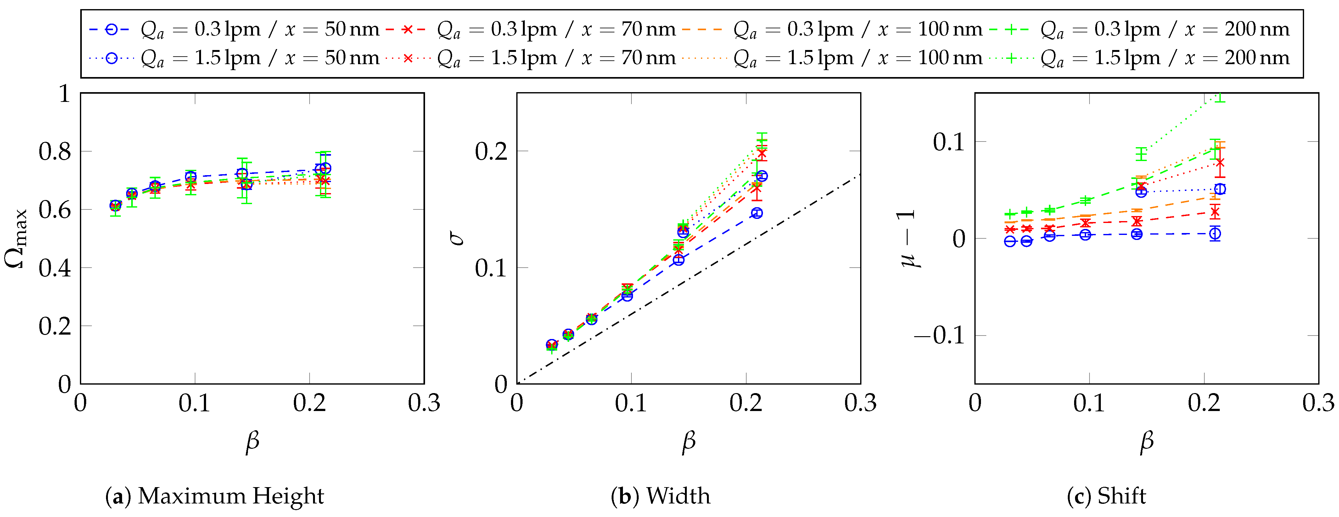
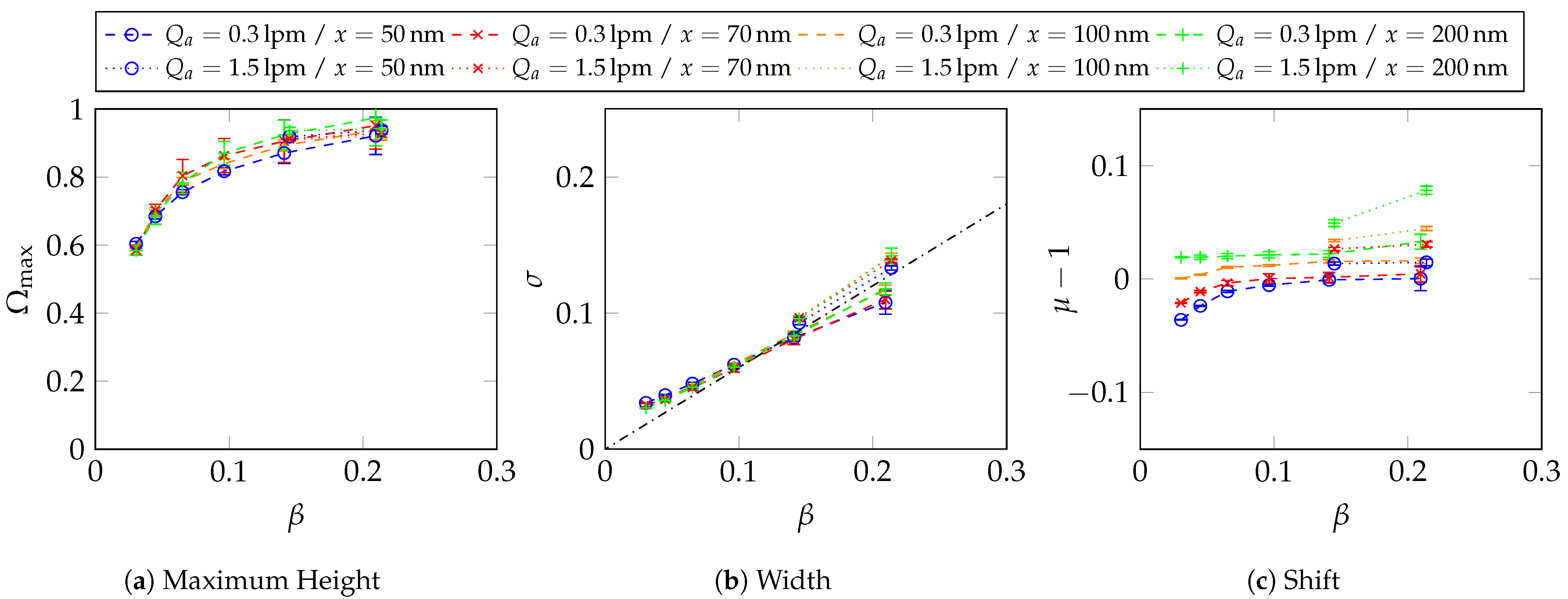
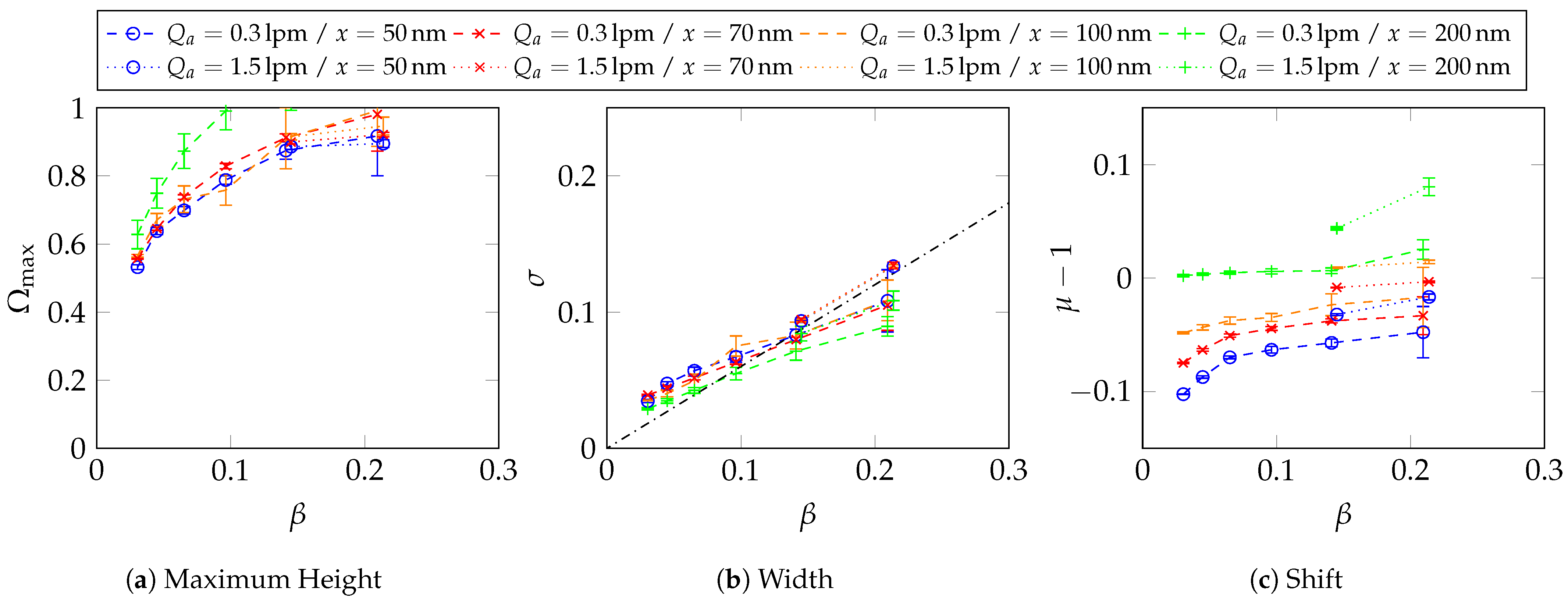
Appendix B. Transfer Function Parameter Determination

As it is very important to know the transfer function of the pre-classifying DMA precisely when measuring the transfer function of the CDMA via a tandem setup (see Equation (13)), this section describes how this DMA transfer function can be determined precisely in advance.
For this purpose, three identical DMAs (Long DMA TSI 3081) were measured in each possible tandem setup arrangement. The aerosol used was a silver aerosol, which was produced as in Section 3. Please keep in mind that Equation (13) is only applicable for broad particle size distributions at the inlet of the first DMA, i.e., the particle density distribution can be considered constant over a classification window of the DMA. Otherwise, the distribution must be included in the calculation. We now assume that all DMAs are identical and consequently have the same transfer function, which can be well described by a Gaussian function [15], i.e., c = e and μ ˜ 1 = μ ˜ 2 . Since μ ˜ 2 is the varied parameter for the data points to fit on, in this special case, μ ˜ 1 is fixed and must be set to one, and the resulting shift then is twice as high. Thus, Equation (15) for two identical DMA’s results in:
n 2 / n 1 = 1 2 · d · exp ( μ ˜ 2 / 2 1 ) 2 2 · e 2
To obtain comparative values that were as valid as possible, the aerosol volume flow rate was varied to 0.3 and 1.5 l / min , and the sheath air volume flow rate was varied to different values. This was done to ensure the most accurate and valid results possible. This method enabled the analysis of different beta values. The series of measurements were conducted at particle sizes of 50, 70, 100, and 200 nm. For every measuring point, the mean value was calculated from three individual measurements, resulting in a measured parameter set for every setting (see Figure A2). To determine the characteristic parameters of every DMA, the mean value of μ ˜ was first determined for every DMA–DMA combination. The c has a linear dependency to β so that a linear regression is applied to obtain a regression constant for every combination, so that c = k · β . Table A1 lists the values for k 2 and μ ˜ 2 for the assumption that the tandem setup consists of two identical DMAs. It can be seen that the values for the combinations differ from each other, but there is some regularity, i.e., all combinations show a significantly broader transfer function since k 2 is considerably larger.
Table A1. Values for k 2 and μ ˜ 2 assuming two identical DMA’s in a tandem setup.
DMA Combination1-21-32-12-33-13-2
k 2 0.67781.01730.69641.04430.86220.8950
μ ˜ 2 1.02821.05681.02611.05040.99000.9891
In order to remove the assumption of identical transfer functions for all DMAs and to obtain individual parameters for every DMA, a system of equations is required. For the widths of the transfer function, we follow by comparing the coefficients of Equations (A1) and (15):
2 · e identical 2 = c 2 + e 2
Therefore:
2 · β 2 · k identical 2 = ( k DMA 1 2 + k DMA 2 2 ) · β 2
Thus, it is possible to set up a system of equations, where 2 · k identical 2 is the solution vector for each combination, while k DMA 1 2 and k DMA 2 2 are the unknown variables.
The same can be done for μ ˜ 2 :
( μ ˜ 2 , identical 1 ) / 2 = μ ˜ DMA 2 μ ˜ DMA 1
Here, ( μ ˜ 2 , identical 1 ) / 2 is the solution vector. Since the DMA’s were interchanged in every direction, the system of equations was overdetermined, so the solution can be determined by least squares regression.
The height a of the transfer function for the pre-classifying DMA is not important, because it cancels out from Equation (15). This yields the parameters resulting for the DMAs, as shown in Table A2.
Table A2. Parameters of the analysed DMA’s.
DMA123
k0.57320.59880.7818
μ ˜ 1.01541.01171.0080
Here, it is shown that DMA1 and DMA2 are very similar, but DMA3 has a much higher value for k, which yields a broader transfer function. This is also proved in Figure A2, Figure A3, Figure A4, Figure A5, Figure A6 and Figure A7, where it can be seen that for the figures where DMA3 is the second DMA, β is much higher, while for the other diagrams, the width β is around the theoretically ideal line (black dashed line).
Moreover, the maximum height of the transfer functions is decreasing with decreasing values for β . This is because for more narrow transfer functions, the influence of diffusion is increasing. There is also a clear tendency from small to large particles at the maximum height, which is caused by diffusion. For some measurement points, the maximum height exceeds one. Here, DMA3 is the pre-classifying DMA. This indicates that there are discrepancies in the determination of the parameters or measurement errors.
The shift does not seem to have major dependencies on the β -values but seems to be influenced by the particle size or the volume flows itself. This is caused by deviations in the applied voltage of the system.
DMA1 appears to have the best properties; thus, it was selected as the pre-classifying DMA for the CDMA transfer function measurements.
Figure A2. Measured transfer function parameters of the the DMA combination 1-2, with 95% confidence interval derived out of three samples.
Powders 04 00011 g0a2
Figure A3. Measured transfer function parameters of the the DMA combination 1-3, with 95% confidence interval derived out of three samples.
Powders 04 00011 g0a3
Figure A4. Measured transfer function parameters of the the DMA combination 2-1, with 95% confidence interval derived out of three samples.
Powders 04 00011 g0a4
Figure A5. Measured transfer function parameters of the the DMA combination 2-3, with 95% confidence interval derived out of three samples.
Powders 04 00011 g0a5
Figure A6. Measured transfer function parameters of the the DMA combination 3-1, with 95% confidence interval derived out of three samples.
Powders 04 00011 g0a6
Figure A7. Measured transfer function parameters of the the DMA combination 3-2, with 95% confidence interval derived out of three samples.
Powders 04 00011 g0a7

Appendix C. Two-Dimensional Property Distribution for Agglomerated Silver Particles Treated at Different Sintering Temperatures

Figure A8. Measurement results for silver particles at a sintering temperature of 250   ° C .
Powders 04 00011 g0a8
Figure A9. Measurement results for silver particles at a sintering temperature of 100   ° C .
Powders 04 00011 g0a9
Figure A10. Measurement results for silver particles at a sintering temperature of 60   ° C .
Powders 04 00011 g0a10

References

  1. Baron, P.A.; Kulkarni, P.; Willeke, K. Aerosol Measurement: Principles, Techniques, and Applications, 3rd ed.; Wiley: Hoboken, NJ, USA, 2011. [Google Scholar]
  2. Friedlander, S.K. Smoke, Dust, and Haze: Fundamentals of Aerosol Dynamics, 2nd ed.; Topics in Chemical Engineering; Oxford University Press: New York, NY, USA, 2000. [Google Scholar]
  3. Colbeck, I. Aerosol Science: Technology and Applications, 2nd ed.; Wiley: Hoboken, NJ, USA, 2013. [Google Scholar]
  4. Park, K.; Dutcher, D.; Emery, M.; Pagels, J.; Sakurai, H.; Scheckman, J.; Qian, S.; Stolzenburg, M.R.; Wang, X.; Yang, J.; et al. Tandem Measurements of Aerosol Properties—A Review of Mobility Techniques with Extensions. Aerosol Sci. Technol. 2008, 42, 801–816. [Google Scholar] [CrossRef]
  5. Rawat, V.K.; Buckley, D.T.; Kimoto, S.; Lee, M.H.; Fukushima, N.; Hogan, C.J. Two dimensional size–mass distribution function inversion from differential mobility analyzer–aerosol particle mass analyzer (DMA–APM) measurements. J. Aerosol Sci. 2016, 92, 70–82. [Google Scholar] [CrossRef]
  6. Buckley, D.T.; Kimoto, S.; Lee, M.H.; Fukushima, N.; Hogan, C.J. Technical note: A corrected two dimensional data inversion routine for tandem mobility-mass measurements. J. Aerosol Sci. 2017, 114, 157–168. [Google Scholar] [CrossRef]
  7. Sipkens, T.A.; Olfert, J.S.; Rogak, S.N. Inversion methods to determine two-dimensional aerosol mass-mobility distributions II: Existing and novel Bayesian methods. J. Aerosol Sci. 2020, 146, 105565. [Google Scholar] [CrossRef]
  8. Broda, K.N.; Olfert, J.S.; Irwin, M.; Schill, G.P.; McMeeking, G.R.; Schnitzler, E.G.; Jäger, W. A novel inversion method to determine the mass distribution of non-refractory coatings on refractory black carbon using a centrifugal particle mass analyzer and single particle soot photometer. Aerosol Sci. Technol. 2018, 52, 567–578. [Google Scholar] [CrossRef]
  9. Sipkens, T.A.; Boies, A.; Corbin, J.C.; Chakrabarty, R.K.; Olfert, J.; Rogak, S.N. Overview of methods to characterize the mass, size, and morphology of soot. J. Aerosol Sci. 2023, 173, 106211. [Google Scholar] [CrossRef]
  10. Tavakoli, F.; Olfert, J.S. Determination of particle mass, effective density, mass–mobility exponent, and dynamic shape factor using an aerodynamic aerosol classifier and a differential mobility analyzer in tandem. J. Aerosol Sci. 2014, 75, 35–42. [Google Scholar] [CrossRef]
  11. Knutson, E.O.; Whitby, K.T. Aerosol classification by electric mobility: Apparatus, theory, and applications. J. Aerosol Sci. 1975, 6, 443–451. [Google Scholar] [CrossRef]
  12. Slowik, J.G.; Stainken, K.; Davidovits, P.; Williams, L.R.; Jayne, J.T.; Kolb, C.E.; Worsnop, D.R.; Rudich, Y.; DeCarlo, P.F.; Jimenez, J.L. Particle Morphology and Density Characterization by Combined Mobility and Aerodynamic Diameter Measurements. Part 2: Application to Combustion-Generated Soot Aerosols as a Function of Fuel Equivalence Ratio. Aerosol Sci. Technol. 2004, 38, 1206–1222. [Google Scholar] [CrossRef]
  13. Tavakoli, F.; Olfert, J.S. An Instrument for the Classification of Aerosols by Particle Relaxation Time: Theoretical Models of the Aerodynamic Aerosol Classifier. Aerosol Sci. Technol. 2013, 47, 916–926. [Google Scholar] [CrossRef]
  14. Rüther, T.N.; Rasche, D.B.; Schmid, H.J. The Centrifugal Differential Mobility Analyser—A New Device for Determination of Two-Dimensional Property Distributions. Aerosol Res. 2025, 3, 65–79. [Google Scholar] [CrossRef]
  15. Rüther, T.N.; Schmid, H.J. Prediction of the transfer function for a Centrifugal Differential Mobility Analyzer by Streamline functions. Aerosol Sci. Technol. 2025; submitted. [Google Scholar]
  16. Rüther, T.N.; Rasche, D.B.; Schmid, H.J. The POCS-Algorithm—An effective tool for calculating 2D particle property distributions via Data Inversion of exemplary CDMA measurement data. Aerosol Sci. 2025; submitted. [Google Scholar]
  17. Allen, M.D.; Raabe, O.G. Slip correction measurements for aerosol particles of doublet and triangular triplet aggregates of spheres. J. Aerosol Sci. 1985, 16, 57–67. [Google Scholar] [CrossRef]
  18. Stolzenburg, M.R. An Ultrafine Aerosol Size Distribution System. Ph.D. Thesis, University of Minnesota, Minneapolis, MN, USA, 1988. [Google Scholar]
  19. Könözsy, L. The kω Shear-Stress Transport (SST) Turbulence Model. In A New Hypothesis on the Anisotropic Reynolds Stress Tensor for Turbulent Flows: Volume I: Theoretical Background and Development of an Anisotropic Hybrid k − ω Shear-Stress Transport/Stochastic Turbulence Model; Springer International Publishing: Cham, Switzerland, 2019; pp. 57–66. [Google Scholar] [CrossRef]
  20. Li, W.; Li, L.; Chen, D.R. Technical Note: A New Deconvolution Scheme for the Retrieval of True DMA Transfer Function from Tandem DMA Data. Aerosol Sci. Technol. 2006, 40, 1052–1057. [Google Scholar] [CrossRef]
  21. DeCarlo, P.F.; Slowik, J.G.; Worsnop, D.R.; Davidovits, P.; Jimenez, J.L. Particle Morphology and Density Characterization by Combined Mobility and Aerodynamic Diameter Measurements. Part 1: Theory. Aerosol Sci. Technol. 2004, 38, 1185–1205. [Google Scholar] [CrossRef]
Figure 1. Cross-section of the CDMA prototype [14].
Powders 04 00011 g001
Figure 2. A 45 ° section of the flow domain used for the calculations, including the boundary conditions.
Powders 04 00011 g002
Figure 3. Cross-sections of the axial flow velocity at different axial coordinates in the proximity of the aerosol inlet. White lines within the displayed planes represent the sources for the plots in Figure 4. The red line at x = 0.151 m indicates the position of the aerosol inlet, which, in this context, represents the region where the aerosol enters the measurement slit.
Powders 04 00011 g003
Figure 4. Plots of the axial velocities for 0 RPM. (Left): at ϕ = 0 with respect to radial coordinate r. (Right): at the middle of the classification gap ( r ¯ = 72.6 mm , see also dotted line left).
Powders 04 00011 g004
Figure 5. Streamlines in the plane at ϕ = 0 ° of the flow domain, for Q a = 0.3 l / min and Q s h = 1.5 l / min . The bottom set of streamlines starts from the aerosol inlet while the upper one ends at the sample outlet.
Powders 04 00011 g005
Figure 6. Plots of the axial velocities for 475 RPM and 2000 RPM . (Left): at ϕ = 0 ° with respect to radial coordinate r. (Right): at the middle of the classification gap ( r ¯ = 72.6 mm , see also dotted line left).
Powders 04 00011 g006
Figure 7. Axial velocity magnitude in the middle plane ( ϕ = 0 ° ) for different rotational speeds.
Powders 04 00011 g007
Figure 8. Relative tangential velocity in the middle plane ( ϕ = 0 ° ) for different rotational speeds.
Powders 04 00011 g008
Figure 9. Representative particle trajectories at the sample outlet. Trajectories labeled in green are successfully sampled. The trajectories labeled in red are not classified.
Powders 04 00011 g009
Figure 10. Ideal two-dimensional transfer function with β = 0.1 and h ˜ = 0.05 . Operating conditions are taken into account by normalization of Z ˜ and τ ˜ by Z * and τ * , respectively. The dashed red lines represent transfer functions for τ ˜ = 0 and Z ˜ = 0 , respectively. The solid red line represents the transfer function of singly charged spherical particles at fixed operating parameters ( ω , U ) .
Powders 04 00011 g010
Figure 11. Comparison of transfer functions of spherical particles at Z ˜ = 0 and τ ˜ = 0 determined by streamline and particle trajectory simulation approaches, respectively. With β = 0.2 and a modal particle size of 100 nm .
Powders 04 00011 g011
Figure 12. Comparison of transfer functions at different operation modes determined by streamline and particle trajectory simulation approaches, respectively. With β = 0.2 and a particle density of 10,490 kg / m 3 .
Powders 04 00011 g012
Figure 13. Schematic of the entire experimental setup: test aerosol production with two tube furnaces (Nabertherm) and an agglomeration tube, as well as the consecutive setup for the measurement of a transfer function consisting of a classifier (TSI 3080) with a DMA (TSI 3081), CDMA and CPC (TSI 3775) [14].
Powders 04 00011 g013
Figure 14. Measured transfer function parameters of the CDMA in ‘DMA mode’ (i.e. for τ ˜ = 0 ) with 95% confidence interval derived out of three independent measurements, corrected for simulated diffusion in the measurement gap, electrical and centrifugal losses.
Powders 04 00011 g014
Figure 15. Measured transfer function parameters of the CDMA operated in ‘AAC mode’ (i.e., for Z ˜ = 0 ) with 95% confidence interval derived out of three independent measurements, corrected for simulated diffusion in the measurement gap, electrical and centrifugal losses.
Powders 04 00011 g015
Figure 16. Measured transfer function parameters of the CDMA for β = 0.2 with Q a = 0.3 lpm at different particle sizes d p with 95% confidence interval derived from three independent measurements, corrected for simulated diffusion in the measurement gap, electrical and centrifugal losses.
Powders 04 00011 g016
Figure 17. Schematic of the experimental setup for investigation of the two-dimensional distribution at different sintering stages: test aerosol production with a tube-furnace (Nabertherm) at 1150 C , an agglomeration tube and a sintering tube-furnace (Nabertherm) at 20   ° C , 60   ° C , 100   ° C , 175   ° C , 250   ° C and 400   ° C . Followed by the CDMA with a classifier (TSI 3080) providing the voltage and sheath air, and a CPC (TSI 3775).
Powders 04 00011 g017
Figure 18. Measurement results for silver particles at different sintering temperatures.
Powders 04 00011 g018
Disclaimer/Publisher’s Note: The statements, opinions and data contained in all publications are solely those of the individual author(s) and contributor(s) and not of MDPI and/or the editor(s). MDPI and/or the editor(s) disclaim responsibility for any injury to people or property resulting from any ideas, methods, instructions or products referred to in the content.

