Article

Increased Extreme Precipitation in Western North America from Cut-Off Lows Under a Warming Climate

1
Department of Atmospheric Sciences, University of Sao Paulo, Sao Paulo 05508-090, Brazil
2
National Centre for Atmospheric Science, Department of Meteorology, University of Reading, Reading RG6 6UR, UK
*
Author to whom correspondence should be addressed.
Meteorology 2025, 4(2), 11; https://doi.org/10.3390/meteorology4020011
Submission received: 5 November 2024 / Revised: 26 January 2025 / Accepted: 3 April 2025 / Published: 9 April 2025

Abstract

:
Cut-off low (COL) pressure systems significantly influence local weather in regions with high COL frequency, particularly in western North America. Nonetheless, future changes in COL frequency, intensity, and precipitation patterns remain uncertain. This study examines projected COL changes and their drivers in western North America under a high greenhouse gas concentration pathway (SSP585) using a multi-model ensemble from CMIP6 and a feature-tracking algorithm. We compare historical simulations (1980–2009) and future projections (2070–2099), revealing a marked increase in COL track density during summer in the northeast Pacific and western United States, while a strong decrease is projected for winter, associated with shifts in jet streams. Climate models project an increase in COL-related precipitation in future climate, with winter and spring experiencing more intense and localized precipitation, while autumn showing a more widespread precipitation pattern. Additionally, there is an increased frequency of extreme precipitation events, though accompanied by large uncertainties. The projected increase in extreme precipitation highlights the need to understand COL dynamics for effective climate adaptation in affected areas. Further research should aim to refine projections and reduce uncertainties, supporting better-informed policy and decision-making.

1. Introduction

The scientific community has increasingly focused on understanding the potential impacts of climate change on various meteorological phenomena, including cut-off low (COL) pressure systems. COLs are synoptic-scale low-pressure systems displaced equatorward from the main westerly flow and are typically associated with Rossby wave breaking [1]. These systems are slow-moving or stationary, often leading to prolonged periods of extreme precipitation. A typical synoptic pattern associated with COLs involves an ascending motion eastward of an upper-level cyclonic potential vorticity (PV) anomaly, which is essential for triggering convection and precipitation [2,3].
Persistent storms associated with COLs have caused severe flooding in Europe and Asia [4,5,6,7,8], while in the Americas, COLs are a major driver of extreme rainfall along the western slopes of the Andes [9,10] and the Rocky Mountains [11,12,13], contributing more than 50% of annual precipitation. In California, COLs have produced substantial rainfall and snowfall, triggering damaging landslides and flooding [14,15]. Despite significant historical analyses, there remains a lack of comprehensive research on projected changes in COL frequency, intensity, and associated precipitation patterns under high-radiative forcing scenarios. Advancing our understanding of these changes is crucial for predicting regional weather patterns and informing policymakers about potential risks to local communities and environmental systems.
Previous studies have extensively documented the climatology and impacts of COLs. Early work by [16] provided a comprehensive climatology of COLs at 200 hPa in the Northern Hemisphere, detailing their frequency and seasonal distribution. Subsequent studies have identified the western United States (U.S.) near 35° N as the most active region for COLs in North America [17,18]. Ref. [19] expanded on these studies by examining the vertical structure and precipitation patterns of COLs in the Mediterranean region. More recent studies, using reanalysis data and advanced methodologies, have further refined our understanding of COLs in both hemispheres [17,18,19,20,21,22,23]. However, uncertainties remain in COL climatology due to variations in detection criteria, atmospheric levels, and datasets used [18,21,24,25].
Recent studies have enhanced our understanding of the dynamical processes and life cycles of COLs, which involve a complex interplay of diabatic processes influencing their intensification and decay [26,27,28]. Additionally, evaluations of climate models indicate significant advancements in simulating COLs, with the sixth generation of Coupled Model Intercomparison Project (CMIP6) models outperforming the earlier CMIP5 simulations [29]. Furthermore, investigations into the effects of El Niño and La Niña on global COL predictability have provided valuable insights [30].
Despite extensive historical analyses of COLs, a substantial gap remains in understanding their response to future climate change. Although some studies have examined future changes in COLs in specific regions, they underscore the need for comprehensive research in other regions. For instance, high-resolution models have projected significant increases in frequency and intensity of mid-tropospheric closed-lows and extreme rainfall events over southern Africa [31]. Similarly, future climate conditions in western Europe could lead to more frequent and severe precipitation events associated with COLs [32,33,34]. In addition, high-intensity COLs with longer lifetimes are expected to become more frequent during the spring over land regions of the Northern Hemisphere [30]. However, these studies are either restricted to specific regions or focus solely on changes in COL frequency, leaving a critical gap in understanding how COLs will affect regional precipitation patterns under future climate scenarios. Addressing this gap is crucial for developing effective climate adaptation and mitigation strategies.
Predicting the future behavior of COLs is challenging due to the numerous interacting factors that influence their regional patterns, including shifts in jet streams, wave breaking, changes in sea surface temperature patterns, land–sea temperature contrasts, and diabatic feedback directly affecting COL dynamics. The strength and position of jet streams, influenced by amplitude waves and split-jet structures, play a crucial role in COL variability. In particular, a weaker subtropical jet increases the COL frequency, while a stronger upstream polar front jet tends to deepen the COL vertical circulation, typically leading to heavier rainfall compared to shallower systems [35]. These dynamics are generally not well represented in state-of-the-art climate models, including higher-resolution models, where an equatorward bias in the Northern Hemisphere jet streams leads to underestimations of COL activity in regions with high observed occurrence [29]. However, several models from the CMIP6 ensemble aim to reduce uncertainty surrounding projected change in the location, intensity and associated precipitation of COLs in the future.
This study addresses the critical gap in the current understanding of future COL behavior in North America by providing projections under a high-radiative forcing scenario (SSP585). Using a multi-model ensemble from CMIP6 and a feature-tracking algorithm, we examine seasonal changes in COL frequency, intensity, and associated precipitation patterns. Employing a COL-centered methodology, we directly measure the impact of climate warming on precipitation associated with COLs in climate model projections. This research offers detailed insights into how COL dynamics and precipitation may change under future climate conditions, particularly in North America’s most active COL region, contributing valuable knowledge to climate science and supporting the development of public policy, as well as mitigation and adaptation strategies under a warming climate.
The key science questions this study seeks to answer include the following:
  • How will COL frequency and intensity change under the highest forcing scenario (SSP585)?
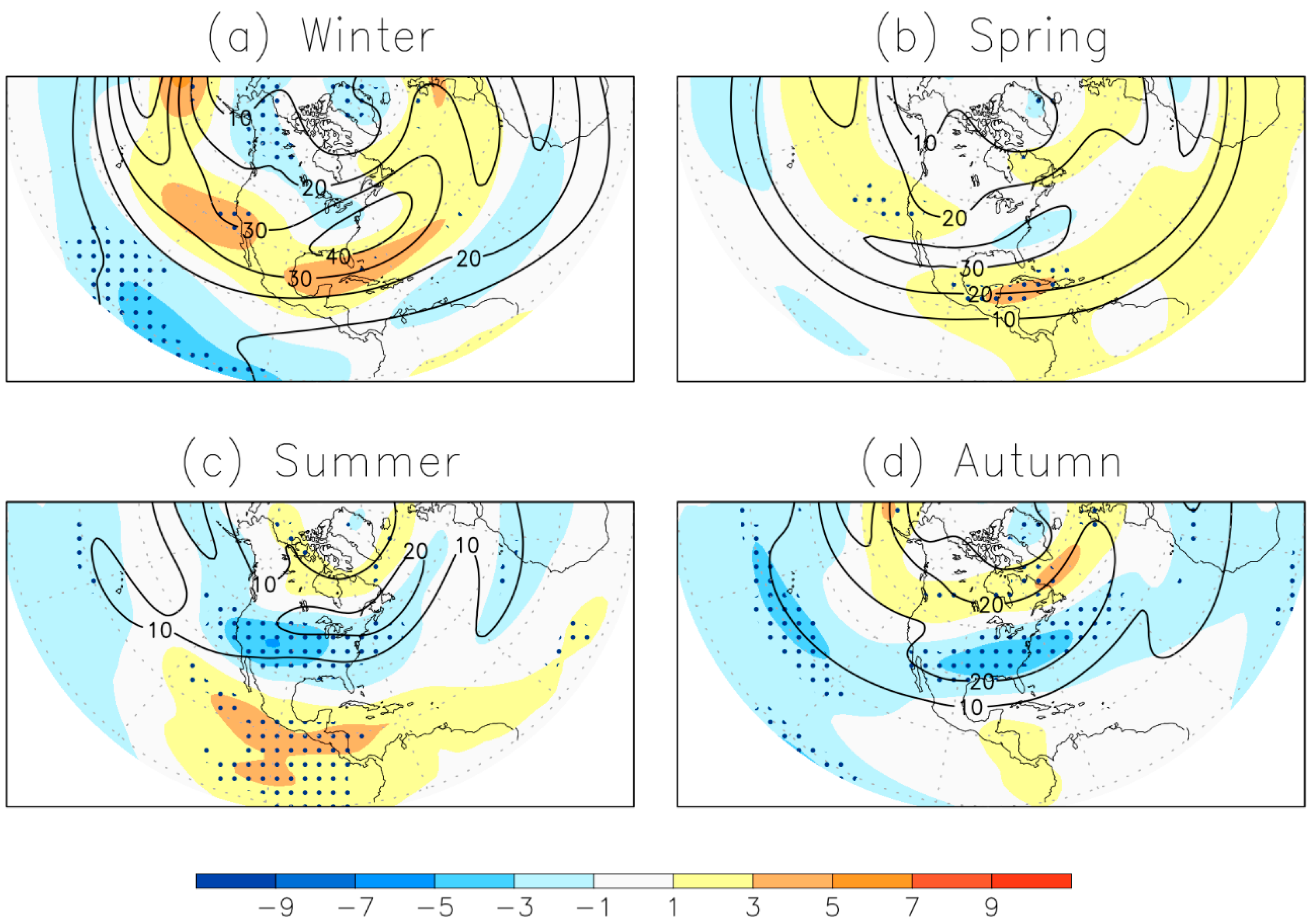
  • How will COL-associated precipitation patterns, including extreme precipitation events, vary seasonally in future climate projections?
  • What dynamical processes drive COL changes, and what uncertainties do models present in these projections?

2. Data and Methods

We use climate model outputs from the CMIP6 [36] archive, specifically from eight high-performing models: ACCESS-CM2, BCC-CSM2-MR, CNRM-CM6-1-HR, MIROC-ES2L, MPI-ESM1-2-HR, MRI-ESM2-0, NESM3, and NorESM2-LM (Table 1). These models, which provide 6-h data at horizontal resolutions ranging from 250 km to 50 km, have shown to have improved performance in simulating COLs compared to CMIP5 models [29]. Analyses are conducted for each season over a historical period (1980–2009) and a future period (2070–2099) under the SSP585 scenario. This late-21st-century high-forcing scenario provides a much higher signal-to-noise ratio, making it easier to detect and isolate significant climate change signals within the climate system.
The model performance is evaluated using data from the European Centre for Medium Range Weather Forecasts (ECMWF) 5th generation reanalysis (ERA5) [37] for the period 1980–2009. Biases in COL locations and associated features (e.g., maximum intensity and precipitation) are assessed by comparing model outputs with the reanalysis data for the historical period. These biases are calculated for each model and ensemble individually as well as for the ensemble multi-model mean. Projected changes in COL features are determined by comparing future projections (2070–2099) with historical simulations (1980–2009).
We applied an objective feature-tracking algorithm, the TRACK algorithm [38,39], to identify COLs in both reanalysis data and climate model simulations. This algorithm has been used extensively in previous studies by the authors [24,25,27,29,30,35]. COLs were identified as features exceeding 1 × 10⁻⁵ s−1 in 6-h 250 hPa relative vorticity. Prior to tracking, data were spectrally filtered to T42 resolution to remove small-scale noise (total wavenumbers > 42) and planetary scales (total wavenumbers < 5), emphasizing the synoptic scale while excluding mesoscale storm systems. The tracking is performed on the sphere by initializing tracks using nearest-neighboring feature points and refining them with a cost function for smoothness with adaptive constraints appropriate for the typical COL motion [24]. A post-tracking filter is applied to ensure the presence of a cut-off circulation by analyzing the 250 hPa horizontal wind components at four offset points around the COL center [24]. Tracks with at least 60% of their points within the region of interest (20–50° N and 140–60° W) and a minimum lifetime of one day were included in the analysis. Seasonal and yearly spatial statistics are computed using spherical kernel estimators to determine track density and mean intensity based on T42 250 hPa vorticity [40].
To identify COL-associated precipitation, we use a radius of influence of 5 geodesic degrees from the vorticity center, capturing precipitation within this radius at each 6-h timestep for both reanalysis and model data. We calculated precipitation from different radii (5°, 10° and 15°) and found that the rate increases with reduced radius. Two approaches are applied to compute the precipitation associated with COLs: (1) maximum precipitation (mm/h), which is calculated at the time of maximum precipitation accumulated over a 6 h period; and (2) cumulative precipitation (mm/event), obtained by summing all precipitation values between the first and last track points of each COL system. Extreme precipitation events, defined as those exceeding the 95th percentile of the historical period (1980–2009) for each ensemble model and reanalysis, are analyzed and categorized as extreme COLs.
The composite structure of COLs is examined using all storms using a system-centered composite method described by Bengtsson et al. [41,42,43]. Atmospheric fields such as horizontal winds, vorticity, and precipitation associated with each COL are sampled onto a 15° longitude–latitude rectangular grid with a 0.5° resolution, initially set up on the equator and then rotated to be centered on the COL’s maximum 250 hPa relative vorticity. This grid setup ensures a fair spatial comparison across different latitudes. Lifecycle composites of precipitation are produced by averaging precipitation around the COL center at various lifecycle stages, centered on the time of maximum intensity. Model biases are calculated by subtracting the values corresponding to the reanalysis from those corresponding to the models across the 15° longitude–latitude domain for each atmospheric field.

3. Results

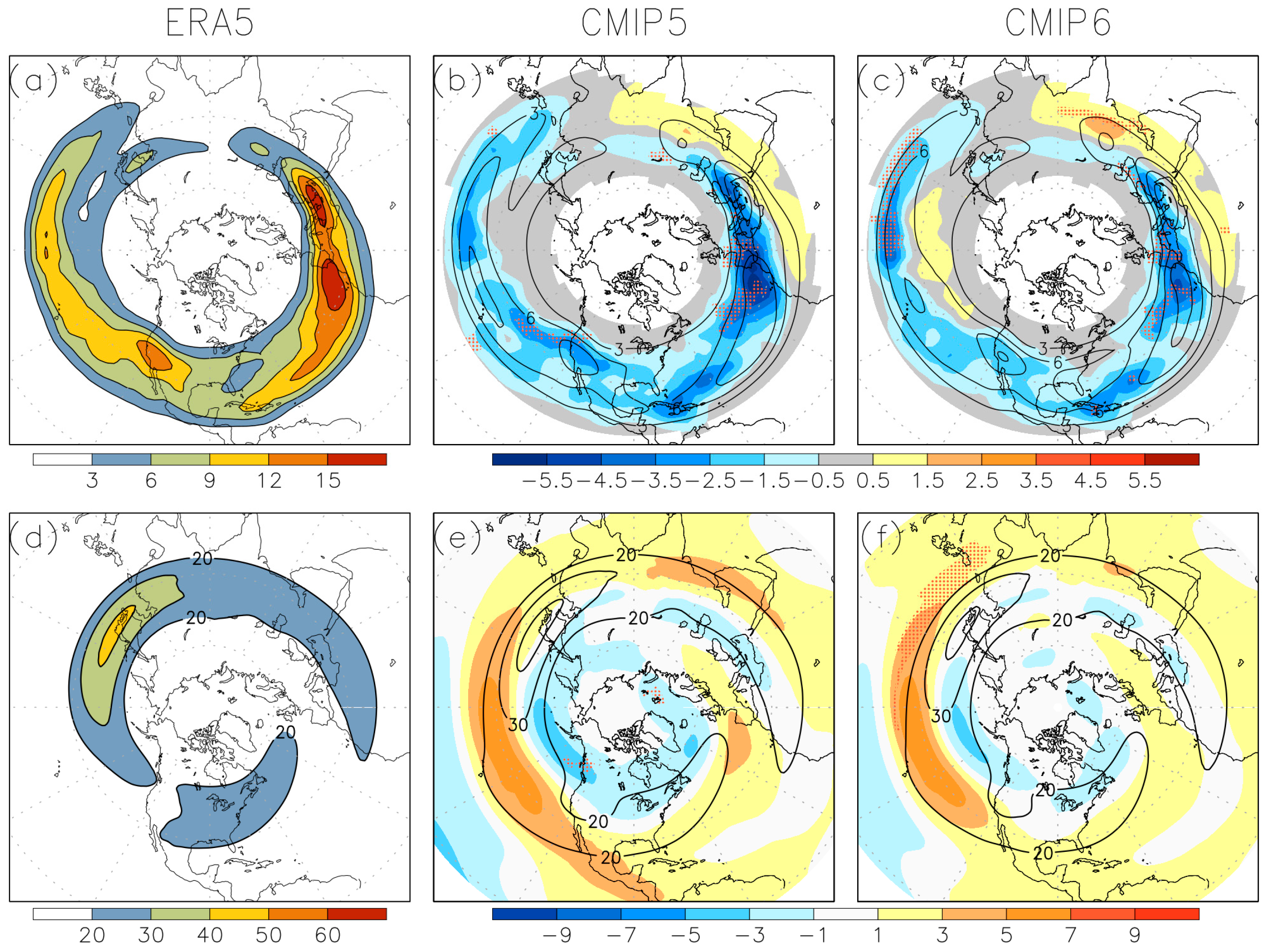
3.1. Northern Hemisphere Perspective of Cut-Off Lows

Building confidence in future climate projections requires that models accurately represent synoptic-scale features with sufficient fidelity. To address this, we begin by summarizing the findings of [29], who assessed the performance of the CMIP5 and CMIP6 historical simulations in simulating COLs. Recent work by [29] shows that CMIP6 models generally simulate COL characteristics more accurately than CMIP5 models when contrasted with reanalyses. Figure 1 exhibits this comparison, showing the annual COL track density of the ERA5 reanalysis (Figure 1a) compared to the multi-model means for CMIP5 (Figure 1b) and CMIP6 (Figure 1c). These comparisons use the same period (1979–2014) and model set (46 models for each CMIP phase) as in [29]. Stippling indicates systematic biases, where all models in each CMIP phase exhibit biases of the same sign.
The Northern Hemisphere COL track density shows similar bias patterns in both CMIP5 and CMIP6 models. However, a significant improvement is evident in CMIP6, where the magnitude of mean biases is considerably lower than in CMIP5, indicating enhanced model performance. The largest track density biases occur in regions of high COL activity, where both CMIP5 and CMIP6 tend to underestimate COL frequency. This underestimation is more significant in CMIP5, whereas CMIP6 models show a reduced bias, suggesting that the CMIP6 better captures COL frequency in these critical regions.
Positive biases, indicating an overestimation of COLs, are more prevalent at lower latitudes, particularly from North Africa across the Middle East and into India. This reflects a persistent equatorward displacement of COL tracks in climate models—a systematic bias that persists in CMIP6. The underestimation of COL track density from the North Pacific into western North America, and from the North Atlantic into central Europe, is likely related to a dipole bias characterized by overly strong winds on the equatorward side and weaker winds on the poleward side of the climatological jet stream. This pattern, shown in Figure 1e,f and demonstrated in [29], leads to a significant underestimation of COL track density in these regions. While the bias in 250 hPa zonal winds is a persistent challenge across climate models, CMIP6 models show a notable reduction in this bias compared to CMIP5, reflecting an improved representation of the jet stream and the associated COL distribution in the latest model generation.

3.2. Cut-Off Low in Western North America

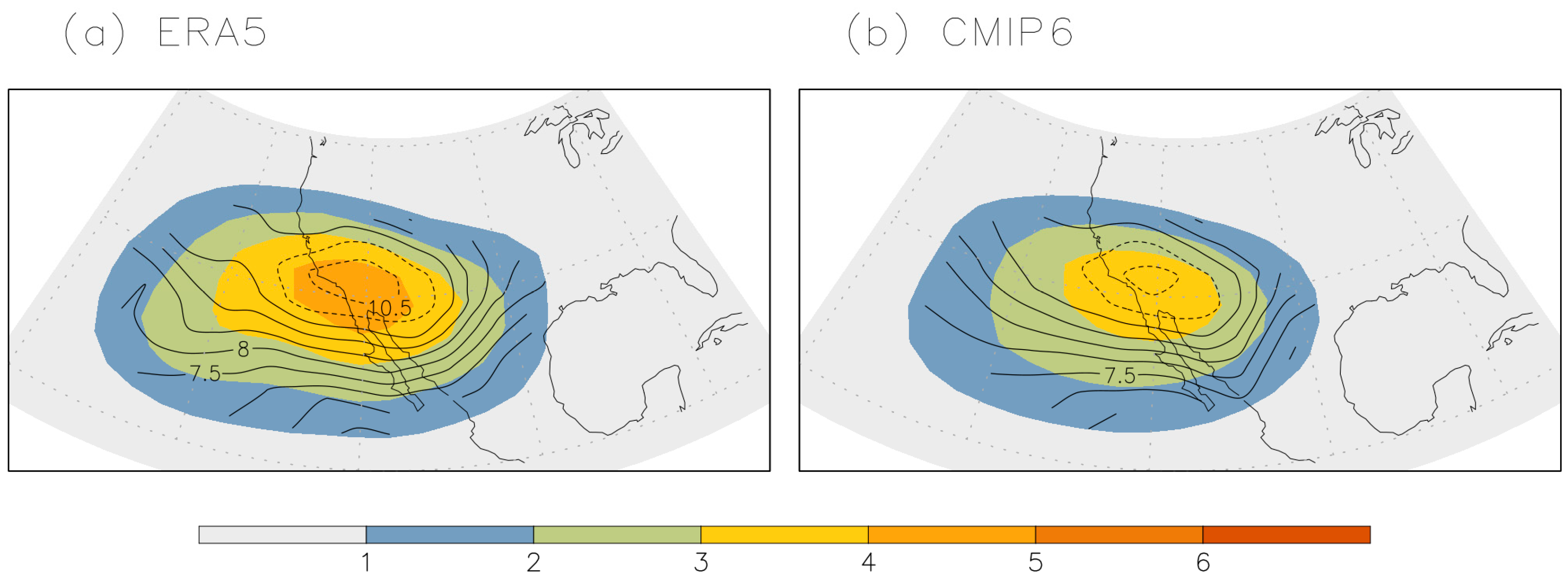
3.2.1. Historical Climate Simulations

To provide a more detailed analysis of the regional climate impacts linked to changes in COLs, this study investigates the ability of CMIP6 models to capture their spatial distribution and intensity over western North America (20–50° N and 140–60° W). The annual track density and mean intensity of COLs (measured by the T42 vorticity at 250 hPa) in CMIP6 historical simulations (Figure 2b) are compared against ERA5 reanalysis (Figure 2a) for the period 1980–2009, using eight CMIP6 models (Table 1). The smaller number of models compared to [29] is due the limited availability of models for future projection scenarios.
Figure 2a shows that the COL activity is concentrated along the western edge of North America, specifically over northwestern Mexico and the southwestern U.S., including California, Arizona, and Nevada. The region of maximum COL intensity closely aligns with areas of highest track density, consistent with previous studies [17,23,44]. While the spatial distribution of track density in the CMIP6 multi-model mean is similar to ERA5, there is a noticeable underestimation in the CMIP6 models, likely due to their coarser horizontal resolution compared to reanalysis data. As shown in Table 1, most CMIP6 models underestimate the number of COL tracks in this region, with the exception of the higher-resolution CNRM-CM6-1-HR model. Despite this underestimation, the mean bias in intensity based on T42 250 hPa relative vorticity is relatively small in the multi-model mean, which enhances confidence in the future projections of COLs.

3.2.2. Projected Response of the Cut-Off Low Activity and Jet Streams Under a Warming Scenario

Building on the evaluation of historical COL activity in CMIP6 models, we now turn to their projected responses under a warming scenario, focusing on changes in the number, intensity, and distribution of COL tracks over western North America by the end of the 21st century. As shown in Table 1, the overall number of COL tracks is expected to decrease slightly by the end of the 21st century, with the multi-model mean reducing from 10.6 to 10.1 tracks per season. This decline is observed in six of the eight models, with particularly notable reductions in CNRM-CM6-1-HR and MIROC-ES2L, while MPI-ESM1-2-HR and NorESM2-LM project slight increases.
Seasonal analysis provides further insight into these projected changes, highlighting distinct patterns in COL characteristics under the SSP585 scenario. Here, it is important to distinguish between track density (Figure 3a–d)—a spatial measure of track distribution—and the overall number of identified tracks. While changes in track number generally reflect shifts in track density, the two metrics are not always correlated, as shown in Tables S1 and S2.
In summer, both track number and track density (Figure 3c) increase markedly, indicating heightened COL activity over the northeast Pacific and western U.S. The multi-model mean shows a 32.2% increase in track number and an 18.4% increase in track density. This trend is robust across most models, with MPI-ESM1-2-HR showing the most substantial increases in both metrics (69.9% in track number, 44.5% in track density). NESM3, however, presents a notable exception, with only a slight rise in track number (5.5%) and a decrease in density (−3.8%).
In winter (Figure 3a), the trend reverses, with both metrics indicating declines in COL activity. The average change in track number is −11.5%, with a corresponding reduction in track density of −16.3%. Track density is a smooth measure, sensitive to track length and location, which can sometimes lead to discrepancies between track number and density changes. For example, while MPI-ESM1-2-HR shows large declines in both track number (−24.1%) and density (−36.2%), CNRM-CM6-1-HR shows a significant decline in track number (−44.0%) but an increase in track density (10.9%) due to projected longer tracks in future climates.
Spring (Figure 3b) exhibits a modest decline in track number (−0.2%) and a more pronounced decrease in track density (−12.2%), though model agreement is inconsistent. NorESM2-LM, for example, projects an increase in track number (20.6%) and density (7.8%), contrasting with models like MIROC-ES2L and MRI-ESM2-0, which show substantial reductions in density (−21.1% and −25.0%, respectively).
Autumn (Figure 3d) presents a more complex picture, with average increases of 12.6% in track number and 2.1% in track density, though model projections vary significantly. While NorESM2-LM and MPI-ESM1-2-HR suggest increases in both metrics, models like MIROC-ES2L and CNRM-CM6-1-HR project reductions. An equatorward shift in COL track density in autumn, extending activity into the Baja California Peninsula, is noted in six models, marking a unique seasonal feature not observed in other periods.
Overall, CMIP6 models generally align on seasonal COL patterns, particularly regarding increased summer and decreased winter activity by the end of the 21st century. However, the inconsistencies between track number and density changes in autumn and spring highlight the variability in regional responses across models and seasons. As illustrated in the CNRM-CM6-1-HR winter projection, longer tracks can result in higher track densities, and vice versa. This model, for instance, projects a decrease in track number but a positive change in track density due to longer tracks in future climates (mean lifetime of 4.0 days) compared to present-day simulations (mean lifetime of 3.3 days).
Changes in the location and intensity of jet streams have important implications for COL characteristics. Previous studies have examined the representation of the northern and southern hemisphere jet streams and their impact on biases in simulated COLs using CMIP5 and CMIP6 historical simulations [29,30]. Notably, positive (negative) mean COL track density biases tend to correspond with negative (positive) upper-tropospheric zonal wind biases, highlighting the role of jet streams in modulating COL behavior.
Figure 4 shows the seasonal response of 250 hPa zonal wind speeds in the SSP585 scenario. CMIP6 models project a notable intensification in the exit region of the wintertime North Pacific jet (Figure 4a), a consistent feature across most models. The upper-tropospheric zonal mean flow accelerates over both western and eastern North America, with the eastern jet showing an equatorward shift, resembling an El Nino-like pattern [45]. The winter jet stream strengthening is primarily associated with a reduced COL track density (see Figure 3a), supported by a significant negative correlation (−0.63) between the two variables. The CMIP6 multi-model projections exhibit a comparable response in spring (Figure 4b), although with weaker wind speed changes than in winter. The spatial response of jet streams across the North Pacific and North Atlantic is similar to that projected by CMIP6 for the SSP245 scenario and by CMIP5 for RCP4.5 [46].
In contrast, the summertime jet stream (Figure 4c) demonstrates a robust weakening in maximum wind speeds, coupled with strengthening to the south and north. In autumn (Figure 4d), the North America jet exhibits a spatial response pattern similar to summer, though the southern jet flank shows a less pronounced strengthening. Unlike winter and spring, the summer weakening of the North America jet correlates with increased COL activity in western North America, though without a statistically significant correlation. Notably, the equatorward shift in the main COL track density in autumn (see Figure 3d) seems to result from weakening along the southern flank of the North America jet. The peak magnitude of jet stream changes reaches approximately 25% (40%) of the mean fields in winter (summer) in regions with the highest COL activity.

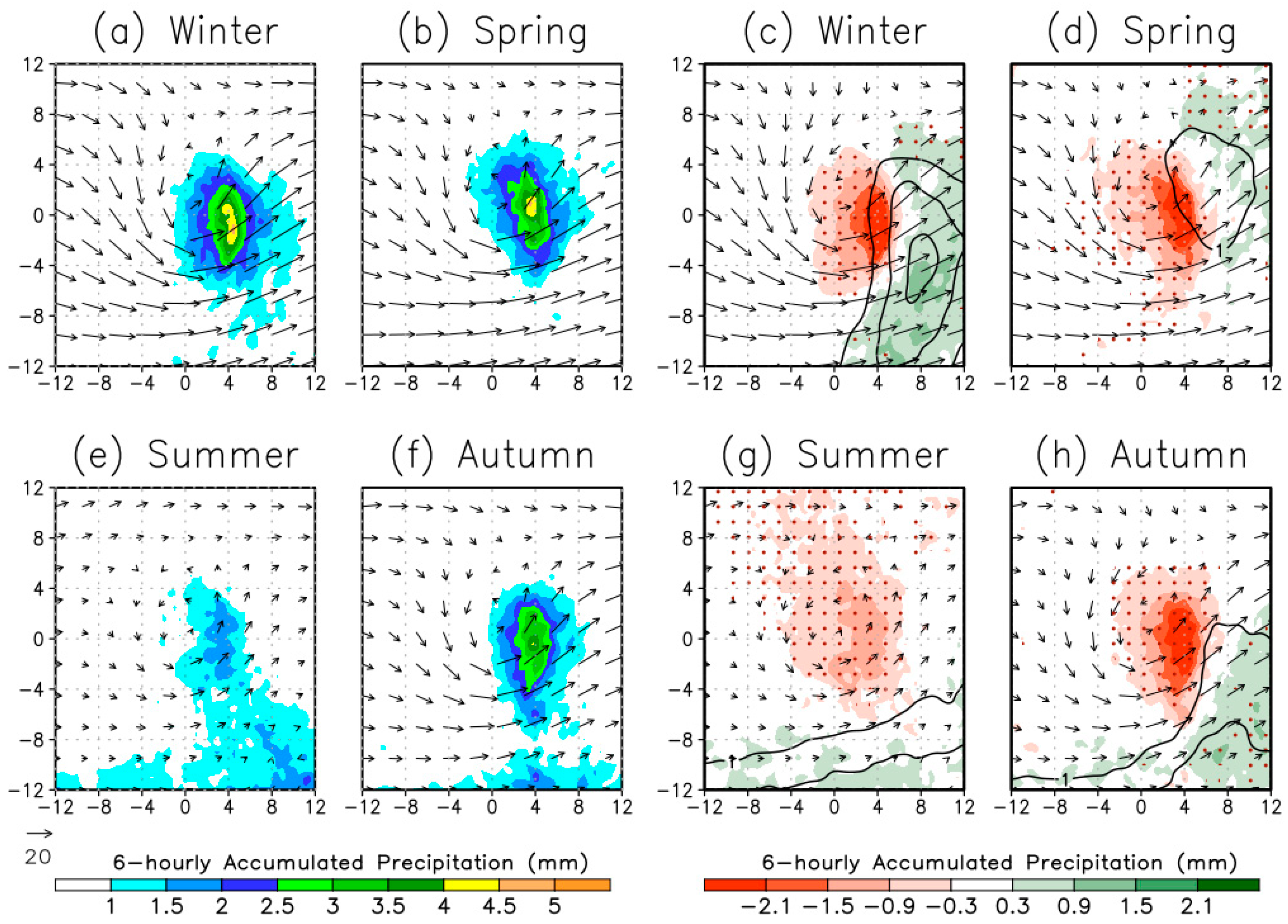
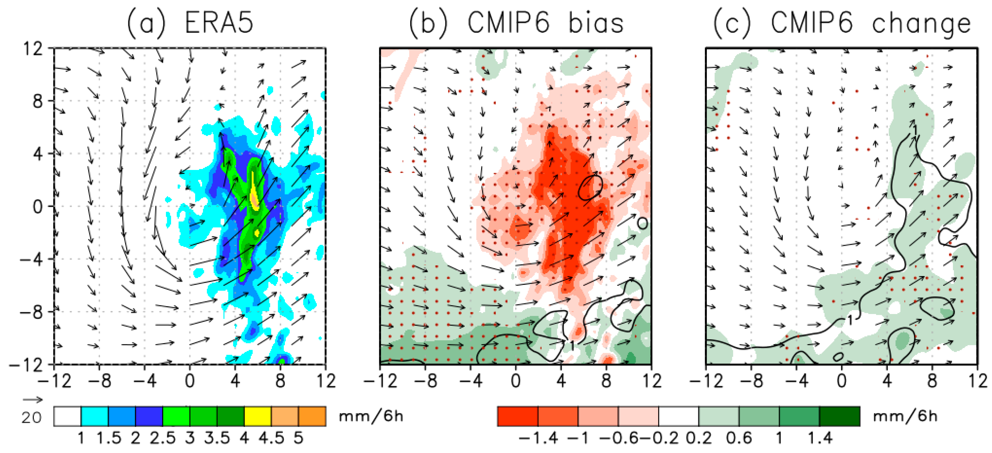
3.2.3. Cut-Off Low Related Precipitation Features

Building on the observed and projected changes in the frequency and spatial distribution of COLs, it is equally critical to understand their associated precipitation patterns to anticipate future impacts accurately. To this end, we first assess how well CMIP6 models reproduce the observed COL-related precipitation, which is essential for evaluating their reliability in future projections. Figure 5 shows the distribution of COL-associated precipitation in western North America, measured by both maximum precipitation rate and accumulated precipitation (see Section 2), with results from historical and future simulations compared against ERA5 reanalysis.
In general, the CMIP6 models capture the maximum precipitation distribution in the historical simulations, though they tend to include a relatively large number of intense precipitation systems (i.e., the upper end of the distribution). The reason for this overestimation is unclear but may be linked to biases in the representation of latent heating, as noted in previous studies of climate models in extratropical regions [47,48]. However, the accumulated precipitation matches closely between the reanalysis and the models, indicating that these models adequately simulate the overall precipitation lifecycle of COLs. This consistency provides confidence in the model simulations, even though their horizontal resolution is coarser than that of the reanalysis data.
In future projections, the overall distribution of COL-associated precipitation remains largely similar to the historical period. However, significant changes are expected in the frequency of extreme precipitation events, which are projected to increase under warmer climate conditions. The most intense precipitation events—often the most damaging—show marked increases, despite the uncertainty indicated by the model spread (red dashed lines). Specifically, precipitation events exceeding the 95th percentile of the historical period (hereafter referred to as extreme COLs), as shown in the inset of Figure 5a, nearly double by the end of the century, with six out of eight models projecting increases of at least 50%.
A similar trend is observed for cumulative precipitation, which accounts for rainfall accumulated over the entire COL lifecycle. Projections suggest an increase in extreme COLs by the end of the 21st century, with all models, except for ACCESS-CM2, showing this trend. On average, there is a 45% increase in the number of extreme precipitation systems, despite a reduction in the total number of COLs (see Table 1). These findings align with projections of reduced COL frequency accompanied by an increase in extreme rainfall events [31,32]. This intensification is possibly influenced by both dynamic and thermodynamic factors, which will be explored in more detail in the following sections of this paper.
To assess the temporal evolution of extreme precipitation events associated with COLs, we analyze trends in maximum precipitation rates exceeding the 95th percentile of the historical period. This approach focuses on the most impactful events, providing a clearer picture of regional changes in their frequency. In this specific analysis, given in Figure 6, we examine the temporal evolution of extreme precipitation events throughout the period from 1980 to 2099, rather than focusing solely on the 2070–2099 period as in previous analyses, to capture trends along the entire period. Climate model projections from the CMIP6 consistently indicate a substantial and increasing trend in the frequency of COL-related extreme precipitation events. By the end of the century, such events are projected to nearly double compared to historical levels, according to the CMIP6 mean. This trend is evident in six out of eight climate models, with BCC-CSM2-MR and CNRM-CM6-1-HR being exceptions. The pronounced increase in extreme precipitation under a high-concentration climate pathway highlights the growing influence of warming on regional rainfall extremes.

3.2.4. Changes in Cut-Off Low Structure

Understanding the structural characteristics of COLs is essential for assessing their dynamics and associated impacts. In this section, we examine the spatial structure of COLs in western North America, focusing on key atmospheric variables such as vorticity, wind patterns and precipitation. By analyzing composite fields from both ERA5 reanalysis and CMIP6 historical simulations, we aim to evaluate the models’ ability to represent these features and identify potential biases that may influence future projections. Figure 7 shows the comparison of 250 hPa horizontal winds and total precipitation for ERA5 and CMIP6 historical simulations. While the wind patterns are consistent between ERA5 and CMIP6, the models slightly underestimate the wind magnitude. However, the CMIP6 models accurately capture the asymmetric horizontal wind distribution around the COLs, with the strongest winds concentrated in the southern quadrant, and successfully reproduce the maximum at 5° to 8° radius from the COL center.
In ERA5, COL-associated precipitation is concentrated primarily ahead of the COL center within a 5° radius, where strong ascent and precipitation typically occur in COLs [43]. The largest precipitation occurs in winter and spring (Figure 7a,b), while a secondary precipitation zone is observed further south in summer and autumn (Figure 7e,f), which may be associated with convective storms linked to the North American monsoon [49]. The composites for CMIP6 show that the total precipitation biases differ spatially (Figure 7c,d,g,h). There is an underestimation near and east of the COL center, while overestimations are found in the surrounding regions, particularly to the east and south. In summer and autumn, the CMIP6 models struggle to reproduce the observed precipitation patterns near the region of maximum precipitation in ERA5. These discrepancies may be due to differences in vertical motion and the release of latent heat, especially in the eastern region of the COL, where substantial precipitation occurs. None of the CMIP6 models accurately capture the summer and autumn precipitation in this critical area.
We now examine the future response of COLs in terms of 250 hPa relative vorticity and precipitation, as shown in Figure 8. Projected changes exhibit clear seasonal and spatial variations. Precipitation is primarily expected to increase in the eastern sectors of COLs, where ascent is strongest, particularly during winter and spring. In winter, precipitation is projected to rise by over 0.7 mm/6 h (~50–70%) in the eastern areas, while decreases are projected in the southern and western regions. Robust model agreement in these areas of increased precipitation supports these projections, despite the overall decline in COL frequency, as shown in Table 1 and Figure 3. Although stronger intensities near the COL center are expected in winter and spring, model agreement on this intensification is lower for winter.
Autumn is the only season where all models consistently project an overall increase in precipitation across the composite domain, with the largest increases occurring in ACCESS-CM2 (+42.9%), NorESM2-LM (+35.5%), and MRI-ESM2-0 (+21.6%). This widespread increase, particularly in the southern sector of COLs, along with a decrease in COL intensity, suggests a potential link to changes in large-scale atmospheric circulation. The projected equatorward shift in COLs in autumn (Figure 3) could strengthen the tropical moisture sources, enhancing latent heat release, which in turn induces an anticyclonic PV anomaly aloft, weakening the upper-level cyclonic circulation [3,50]. Thermodynamic factors likely affect these precipitation changes, reinforcing the role of diabatic processes in weakening COLs [27,51].
The precipitation changes in summer are less intense and more spatially localized. There is a slight weakening of the COL center, with minor increases in precipitation in the east and south quadrants. The changes in vorticity and precipitation during summer are not as pronounced as those observed in other seasons, potentially due to weaker intensities typical of summer. This may contribute to the relatively low model agreement.

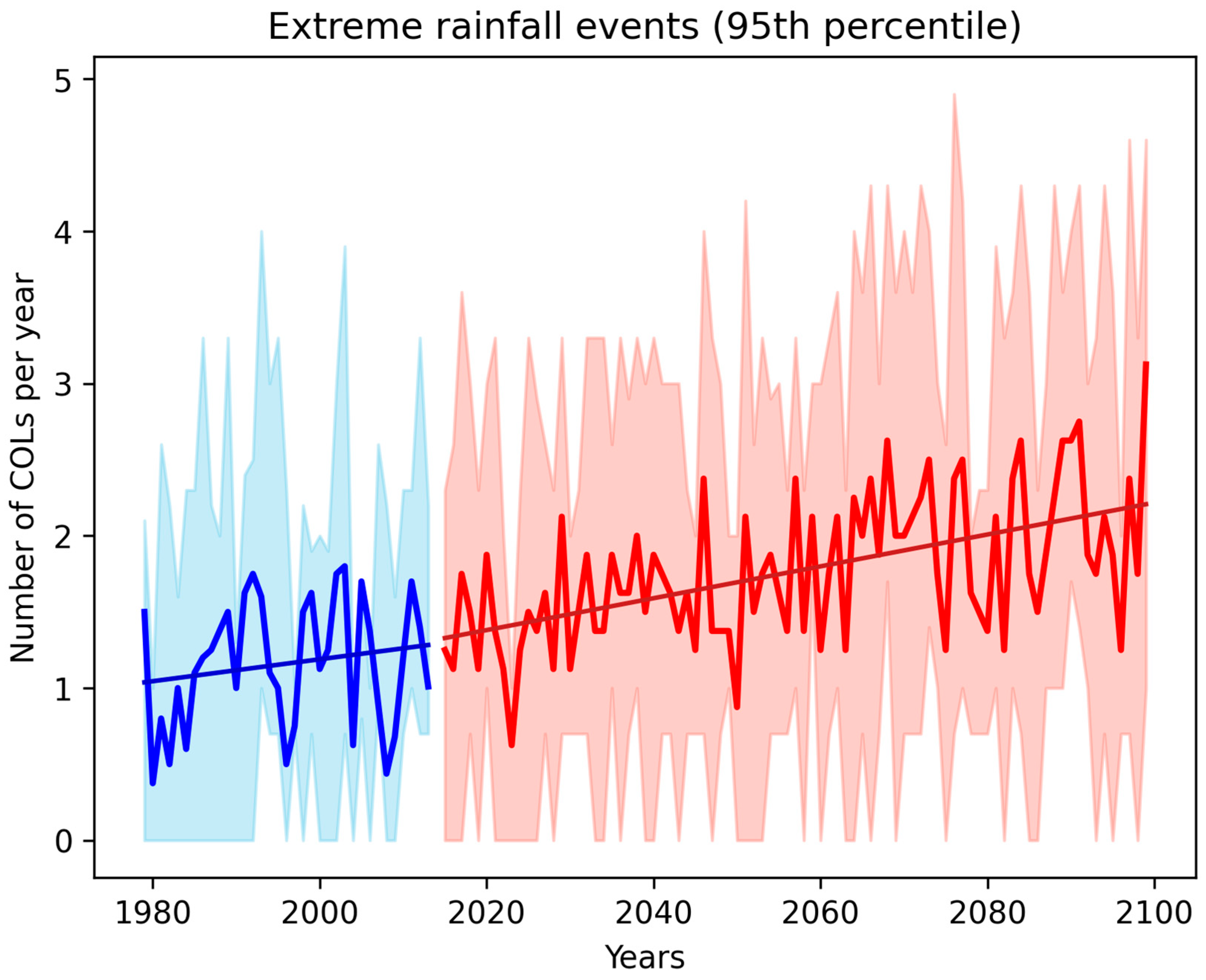
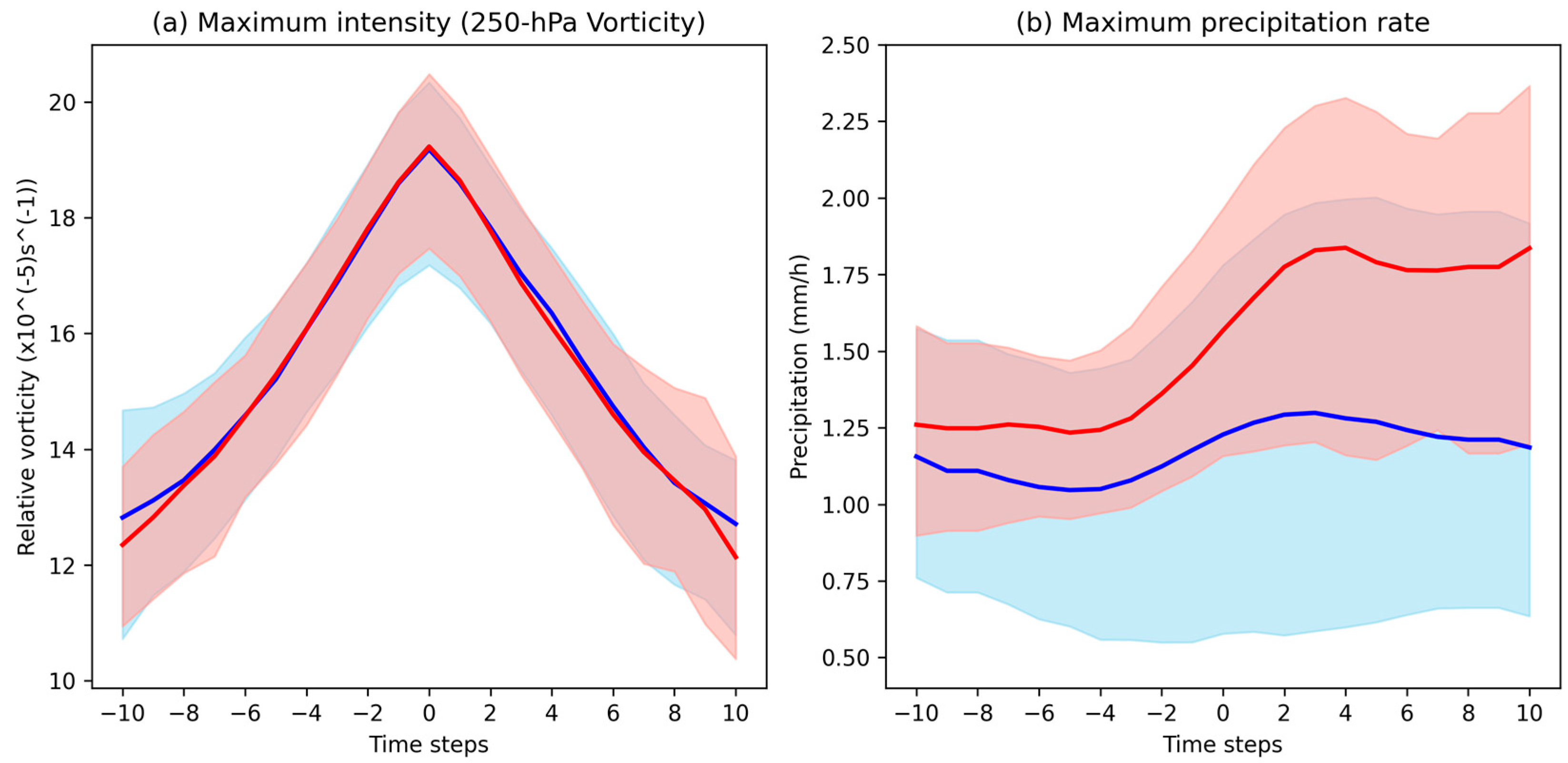
3.2.5. Effect of Climate Warming on the Extreme Precipitation in Cut-Off Lows

As a climate warming influences atmospheric moisture availability, an essential factor for rainfall intensity, it is important to explore how these changes might impact extreme precipitation events associated with COLs. As shown in Figure 7, the CMIP6 models tend to underestimate precipitation within the core of high precipitation areas while overestimating it along the southern flanks of the COL. The ERA5 reanalysis for extreme COL events (95th percentile) (Figure 9a) indicates that the most intense precipitation occurs to the east and northeast of the COL center, a pattern similar to those shown in the seasonal analysis but with higher values. Precipitation biases in CMIP6 historical simulations relative to ERA5 (Figure 9b) are concentrated in these regions, indicating greater uncertainties in the representation of extreme COL precipitation. The pronounced underrepresentation of extreme precipitation could arise from limitations in physical parameterizations, coarse model resolution, or insufficient ensemble size, which are useful to reduce uncertainties and provide an accurate ensemble mean [52,53].
In future projections (Figure 9c), extreme precipitation shifts farther from the COL center, particularly to the east and south, which might be related to enhanced moisture inflow from lower latitudes. Model agreement on the projected increase in extreme precipitation provides reasonable confidence, though uncertainties remain regarding the magnitude due to persistent biases in extreme event representation.
We have demonstrated that CMIP6 models effectively capture precipitation patterns in COLs in the western North America, despite some systematic biases. We now examine potential changes in lifecycle precipitation under a warmer climate, focusing on extreme COL events (95th percentile) to understand the behavior of extreme precipitation. Each COL is centered on the time it reaches peak intensity, based on the T42 250 hPa vorticity, using historical simulations and future projections. Figure 10a shows minimal variation in vorticity for extreme COLs, with only a slight increase in peak intensity in future projections. However, when considering all COL systems, a more pronounced increase in intensity is observed under future climate conditions.
Figure 10b indicates that, consistent with previous studies on Southern Hemisphere COLs [9,43,54], maximum precipitation occurs after peak intensity. In future projections, the rate of precipitation increase is more pronounced than in the historical period, with an average rise of about 44% across all models during the decay stage. Notably, more precipitation is projected for systems with shorter lifetimes in a warmer climate, suggesting a shift toward more intense, short-duration precipitation events, potentially heightening weather-related hazards. However, the mechanisms driving this rapid increase in precipitation remain unclear.

4. Discussion and Conclusions

This study has evaluated the capabilities of CMIP6 models in simulating the characteristics and impacts of COLs in western North America, a region vulnerable to COLs and changes in precipitation in the future. These results corroborate previous findings that CMIP6 models offer a more realistic representation of COL features compared to CMIP5 models, particularly in terms of track density and intensity, with a reduced underestimation in regions of high COL occurrence. While systematic biases persist—most notably in the equatorward displacement of COL tracks—CMIP6 models exhibit improved performance, especially in capturing the frequency of COLs in regions of high activity.
In terms of COL structure, CMIP6 models accurately capture the asymmetric horizontal wind distribution around COL systems, though they show limitations in representing precipitation patterns. Precipitation is significantly underestimated near and east of the COL center and overestimated in surrounding regions. This underestimation near the COL core may be attributed to the models’ poor representation of diabatic processes, which are key to COL dynamics. Latent heat release, known to weaken upper-level cyclonic PV anomalies (e.g., [2]), could be suppressed by the overestimated vorticities in winter and spring COLs, thereby contributing to the precipitation bias. However, this hypothesis does not explain the weaker simulated intensities observed in autumn COLs.
We acknowledge the potential for additional sources of bias in coupled climate models, particularly those associated with atmosphere-ocean latent heat fluxes that influence precipitation-triggering processes, as highlighted in previous studies (e.g., [55,56,57]). Errors in radiative forcings, such as surface downwelling longwave radiation and downward surface shortwave radiation, both critical for precipitation processes, may also contribute to the dry bias near the COL core (e.g., [55,57]). Additionally, biases arising from coarse resolution, imperfect boundary conditions, parameterizations, and inaccuracies in representing physical processes are extensively documented in the literature (e.g., [58,59,60]).
Addressing these biases requires further investigation into key processes driving precipitation (e.g., vertical motion, latent heating, and PV modification) to better understand their impact on future projections. Improved model accuracy may require higher-resolution simulations, especially with convection-permitting models which can more effectively resolve these features and reduce associated uncertainties.
Seasonal responses of COLs to climate change reveal distinct patterns. A decline in COL frequency is projected for winter, while an increase is expected in summer. These changes are suggested to correlate with shifts in the upper-tropospheric jet streams, where intensification in winter is linked to reduced COL activity, whereas weakening in summer is associated with increased COL activity. Winter precipitation, particularly in the eastern flank of COLs, is projected to rise by approximately 50–70%. Autumn also shows consistent increases, especially in the southern sector of COLs, despite a decline in vorticity intensity. This suggests a potential link to changes in large-scale atmospheric circulation, with the equatorward shift in COLs enhancing tropical moisture source. This shift could induce an anticyclonic PV anomaly aloft, reinforcing the role of diabatic processes in weakening COLs.
Although the overall number of COL tracks is projected to decrease slightly under future climate conditions, associated precipitation is expected to increase. Extreme precipitation events (those exceeding the 95th percentile) are projected to nearly double by the end of the century, with robust model agreement on this trend. The increase in extreme precipitation will likely occur farther from the COL center, particularly toward the east and south, potentially due to enhanced moisture inflow from lower latitudes. A significant increase in precipitation is projected during the decay stage, with an average rise of 44%. Additionally, COLs with shorter lifetimes are expected to produce larger amounts of precipitation in a warmer climate, indicating a shift toward more intense, short-duration precipitation events, thereby increasing weather-related hazards. These findings are consistent with previous studies [31,32,33], which also indicate an increase in COL-related precipitation under warming scenarios. However, uncertainties remain in the representation of extreme precipitation which may arise from limitations in physical parameterizations, coarse model resolution, or the insufficient size of model ensembles.
For future research, employing higher-resolution models, such as HighResMIP (~25–50 km) and kilometer scale models with horizontal resolutions of less than 10 km [61], is crucial for better representing the physical processes and reducing uncertainties in projections of COL behavior under climate change. Comparative analyses across different forcing scenarios could offer valuable insights into the potential range of changes in COL characteristics and their associated impacts. Furthermore, examining how variations in jet stream strength and position affect COL dynamics is essential, as jet streams play an important role in the development and behavior of COLs. Additional studies are needed to explore the interplay between subtropical and polar jets and how their changing characteristics may influence COLs.
As we move toward the next climate assessment (CMIP7), it is worth noting that the upcoming HighResMIP CMIP7 protocol is expected to include historical and future simulations covering the 1950–2100 period, which is longer than the current HighResMIP CMIP6 simulations. Additionally, the Destination Earth initiative (DestinE) and EERIE [62] will provide much higher resolutions (5 to 10 km). Addressing these issues is key to refining projections of COL intensity and precipitation patterns. Further investigations are needed to clarify the implications of these projected changes for regional weather hazards and overall climate impacts.

Supplementary Materials

The following supporting information can be downloaded at: https://www.mdpi.com/article/10.3390/meteorology4020011/s1, Table S1: Percentage change in the number of identified 250 hPa COL tracks for each CMIP6 model across the seasons (Spring, Summer, Autumn, Winter) within the region of 20–50° N and 140–60° W. The percentage change is calculated as the difference between the future period (2070–2099) and the historical period (1980–2009); Table S2: Percentage change in the density of identified 250-hPa COL tracks for each CMIP6 model across the seasons (Spring, Summer, Autumn, Winter) within the region of 20°–50° N and 140°–60° W. The percentage change is calculated as the difference between the future period (2070–2099) and the historical period (1980–2009).

Author Contributions

Conceptualization, H.P.; methodology, H.P. and K.H.; software, K.H.; validation, H.P.; formal analysis, H.P.; investigation, H.P.; resources, H.P. and T.A.; data curation, H.P.; writing—original draft preparation, H.P.; writing—review and editing, H.P., T.A. and K.H.; visualization, H.P.; supervision, T.A.; project administration, T.A.; funding acquisition, T.A. All authors have read and agreed to the published version of the manuscript.

Funding

This research was funded by CNPq (Conselho Nacional de Desenvolvimento Científico e Tecnológico), grant number 151225/2023-0 and FAPESP (Fundação de Amparo à Pesquisa do Estado de São Paulo), grant number 2023/10882-2.

Institutional Review Board Statement

Not applicable.

Informed Consent Statement

Not applicable.

Data Availability Statement

The data used in this study are sourced from the World Climate Research Programme’s Working Group on Coupled Modelling and are freely available through the Earth System Grid Federation (ESGF) at https://esgf-index1.ceda.ac.uk/search/cmip6-ceda/, accessed on 4 April 2025. ERA5 data were obtained from the Copernicus Climate Change Service’s Climate Data Store, accessible at https://cds.climate.copernicus.eu/, accessed on 4 April 2025.

Conflicts of Interest

The authors declare no conflicts of interest. The funders had no role in the design of the study; in the collection, analyses, or interpretation of data; in the writing of the manuscript; or in the decision to publish the results.

References

  1. Ndarana, T.; Waugh, D.W. The link between cut-off lows and Rossby wave breaking in the Southern Hemisphere. Q. J. R. Meteorol. Soc. 2010, 136, 869–885. [Google Scholar] [CrossRef]
  2. Hoskins, B.J.; McIntyre, M.E.; Robertson, A.W. On the use and significance of isentropic potential vorticity maps. Q. J. R. Meteorol. Soc. 1985, 111, 877–946. [Google Scholar] [CrossRef]
  3. Davis, C.A.; Emanuel, K.A. Potential vorticity diagnostics of cyclogenesis. Mon. Weather Rev. 1991, 119, 1929–1953. [Google Scholar] [CrossRef]
  4. Zhao, S.; Sun, J. Study on cut-off low-pressure systems with floods over Northeast Asia. Meteorol. Atmos. Phys. 2007, 96, 159–180. [Google Scholar] [CrossRef]
  5. Awan, N.K.; Formayer, H. Cutoff low systems and their relevance to large-scale extreme precipitation in the European Alps. Theor. Appl. Climatol. 2017, 129, 149–158. [Google Scholar] [CrossRef]
  6. Ibebuchi, C.C. Patterns of Atmospheric Circulation in Western Europe Linked to Heavy Rainfall in Germany: Preliminary Analysis into the 2021 Heavy Rainfall Episode. Theor. Appl. Climatol. 2022, 148, 269–283. [Google Scholar] [CrossRef]
  7. Kramers, T. Multidecadal Analysis of Spatiotemporal Distribution and Severity of Cut-Off Lows Over Europe. Master’s Thesis, Wageningen University & Research, Wageningen, The Netherlands, 2024. [Google Scholar]
  8. Yamamoto, K.; Iga, K.; Yamazaki, A. Mergers as the maintenance mechanism of cutoff lows: A case study over Europe in July 2021. Mon. Weather Rev. 2024, 152, 1241–1256. [Google Scholar] [CrossRef]
  9. Bozkurt, D.; Rondanelli, R.; Garreaud, R.; Arriagada, A. Impact of warmer eastern tropical Pacific SST on the March 2015 Atacama floods. Mon. Weather Rev. 2016, 144, 4441–4460. [Google Scholar] [CrossRef]
  10. Aceituno, P.; Boisier, J.P.; Garreaud, R.; Rondanelli, R.; Rutllant, J.A. Climate and weather in Chile. In Water Resources of Chile; Springer: Cham, Switzerland, 2021; pp. 7–29. [Google Scholar]
  11. Oakley, N.S.; Redmond, K.T. A climatology of 500-hPa closed lows in the Northeastern Pacific Ocean, 1948–2011. J. Appl. Meteorol. Climatol. 2014, 53, 1578–1592. [Google Scholar] [CrossRef]
  12. Abatzoglou, J.T. Contribution of cutoff lows to precipitation across the United States. J. Appl. Meteorol. Climatol. 2016, 55, 893–899. [Google Scholar] [CrossRef]
  13. Barbero, R.; Abatzoglou, J.T.; Fowler, H.J. Contribution of large-scale midlatitude disturbances to hourly precipitation extremes in the United States. Clim. Dyn. 2019, 52, 197–208. [Google Scholar] [CrossRef]
  14. Oakley, N.S.; Lancaster, J.T.; Hatchett, B.J.; Stock, J.; Ralph, F.M.; Roj, S.; Lukashov, S. A 22-year climatology of cool season hourly precipitation thresholds conducive to shallow landslides in California. Earth Interact. 2018, 22, 1–35. [Google Scholar] [CrossRef]
  15. Characteristics and Impacts of the April 4–11 2020 Cutoff Low Storm in California. Available online: https://cw3e.ucsd.edu/characteristics-and-impacts-of-the-april-4-11-2020-cutoff-low-storm-in-california/ (accessed on 12 January 2025).
  16. Kentarchos, A.S.; Davies, T.D. A climatology of cut-off lows at 200 hPa in the Northern Hemisphere, 1990–1994. Int. J. Climatol. 1998, 18, 379–390. [Google Scholar] [CrossRef]
  17. Sprenger, M.; Wernli, H.; Bourqui, M. Stratosphere–troposphere exchange and its relation to potential vorticity streamers and cutoffs near the extratropical tropopause. J. Atmos. Sci. 2007, 64, 1587–1602. [Google Scholar] [CrossRef]
  18. Nieto, R.; Sprenger, M.; Wernli, H.; Trigo, R.M.; Gimeno, L. Identification and climatology of cut-off lows near the tropopause. Ann. N. Y. Acad. Sci. 2008, 1146, 256–290. [Google Scholar] [CrossRef]
  19. Porcù, F.; Carrassi, A.; Medaglia, C.M.; Prodi, F.; Mugnai, A. A study on cut-off low vertical structure and precipitation in the Mediterranean region. Met. Atmos. Phys. 2007, 96, 121–140. [Google Scholar] [CrossRef]
  20. Fuenzalida, H.A.; Sánchez, R.; Garreaud, R.D. A climatology of cutoff Lows in the Southern Hemisphere. J. Geophys. Res. Atmos. 2005, 110, D18. [Google Scholar] [CrossRef]
  21. Reboita, M.S.; Nieto, R.; Gimeno, L.; Da Rocha, R.P.; Ambrizzi, T.; Garreaud, R.; Krüger, L.F. Climatological features of cutoff low systems in the Southern Hemisphere. J. Geophys. Res. Atmos. 2010, 115, D17. [Google Scholar] [CrossRef]
  22. Pinheiro, H.R.; Hodges, K.I.; Gan, M.A.; Ferreira, N.J. A new perspective of the climatological features of upper-level cut-off lows in the Southern Hemisphere. Clim. Dyn. 2017, 48, 541–559. [Google Scholar] [CrossRef]
  23. Muñoz, C.; Schultz, D.; Vaughan, G. A Midlatitude Climatology and Interannual Variability of 200- and 500-hPa Cut-Off Lows. J. Clim. 2020, 33, 2201–2222. [Google Scholar] [CrossRef]
  24. Pinheiro, H.R.; Hodges, K.I.; Gan, M.A. Sensitivity of identifying cut-off lows in the Southern Hemisphere using multiple criteria: Implications for numbers, seasonality and intensity. Clim. Dyn. 2019, 53, 6699–6713. [Google Scholar] [CrossRef]
  25. Pinheiro, H.R.; Hodges, K.I.; Gan, M.A. An intercomparison of subtropical cut-off lows in the Southern Hemisphere using recent reanalyses: ERA-Interim, NCEP-CFRS, MERRA-2, JRA-55, and JRA-25. Clim. Dyn. 2020, 54, 777–792. [Google Scholar] [CrossRef]
  26. Portmann, R.; Crezee, B.; Quinting, J.; Wernli, H. The complex life cycles of two long-lived potential vorticity cut-offs over Europe. Q. J. R. Meteorol. Soc. 2018, 144, 701–719. [Google Scholar] [CrossRef]
  27. Pinheiro, H.R.; Hodges, K.I.; Gan, M.A.; Ferreira, S.H.; Andrade, K.M. Contributions of downstream baroclinic development to strong Southern Hemisphere cut-off lows. Q. J. R. Meteorol. Soc. 2022, 148, 214–232. [Google Scholar] [CrossRef]
  28. Nie, Y.; Wu, J.; Zuo, J.; Ren, H.L.; Scaife, A.A.; Dunstone, N.; Hardiman, S.C. Subseasonal prediction of early-summer Northeast Asian cut-off lows by BCC-CSM2-HR and GloSea5. Adv. Atmos. Sci. 2023, 40, 2127–2134. [Google Scholar] [CrossRef]
  29. Pinheiro, H.; Ambrizzi, T.; Hodges, K.; Gan, M.; Andrade, K.; Garcia, J. Are Cut-off Lows simulated better in CMIP6 compared to CMIP5? Clim. Dyn. 2022, 59, 2117–2136. [Google Scholar] [CrossRef]
  30. Pinheiro, H.R.; Ambrizzi, T.; Hodges, K.I.; Gan, M.A. Understanding the El Niño southern oscillation effect on cut-off lows as simulated in forced SST and fully coupled experiments. Atmosphere 2022, 13, 1167. [Google Scholar] [CrossRef]
  31. Engelbrecht, F.A.; Dyson, L.L. High-resolution model-projected changes in mid-tropospheric closed-lows and extreme rainfall events over southern Africa. Int. J. Climatol. 2013, 33, 173–187. [Google Scholar] [CrossRef]
  32. Ferreira, R.N. Cut-off lows and extreme precipitation in eastern Spain: Current and future climate. Atmosphere 2021, 12, 835. [Google Scholar] [CrossRef]
  33. Thompson, V.; Coumou, D.; Galfi, V.M.; Happé, T.; Kew, S.; Pinto, I.; Philip, S.; de Vries, H.; van der Wiel, K. Changing dynamics of Western European summertime cut-off lows: A case study of the July 2021 flood event. Atmos. Sci. Lett. 2024, 25, e1260. [Google Scholar] [CrossRef]
  34. Mishra, A.N.; Maraun, D.; Schiemann, R.; Hodges, K.; Zappa, G. Climate Change’s Influence on Cut-off Lows in the Future. In Proceedings of the EGU General Assembly 2024, EGU24-19896. Vienna, Austria, 14–19 April 2024. [Google Scholar] [CrossRef]
  35. Pinheiro, H.R.; Hodges, K.I.; Gan, M.A. Deepening mechanisms of cut-off lows in the Southern Hemisphere and the role of jet streams: Insights from eddy kinetic energy analysis. Weather Clim. Dynam. 2024, 5, 881–894. [Google Scholar] [CrossRef]
  36. Eyring, V.; Bony, S.; Meehl, G.A.; Senior, C.A.; Stevens, B.; Stouffer, R.J.; Taylor, K.E. Overview of the Coupled Model Intercomparison Project Phase 6 (CMIP6) experimental design and organization. Geosci. Model Dev. 2016, 9, 1937–1958. [Google Scholar] [CrossRef]
  37. Hersbach, H. ERA5 reanalysis is in production. ECMWF Newsl. 2016, 147, 5. [Google Scholar]
  38. Hodges, K.I. Feature tracking on the unit sphere. Mon. Weather Rev. 1995, 123, 3458–3465. [Google Scholar] [CrossRef]
  39. Hodges, K.I. Adaptive constraints for feature tracking. Mon. Weather Rev. 1999, 127, 1362–1373. [Google Scholar] [CrossRef]
  40. Hodges, K.I. Spherical nonparametric estimators applied to the UGAMP model integration for AMIP. Mon. Weather Rev. 1996, 124, 2914–2932. [Google Scholar] [CrossRef]
  41. Bengtsson, L.; Hodges, K.I.; Esch, M.; Keenlyside, N.; Kornblueh, L.; Luo, J.J.; Yamagata, T. How may tropical cyclones change in a warmer climate? Tellus A Dyn. Meteorol. Oceanogr. 2007, 59, 539–561. [Google Scholar] [CrossRef]
  42. Bengtsson, L.; Hodges, K.I.; Keenlyside, N. Will extratropical storms intensify in a warmer climate? J. Climate 2009, 22, 2276–2301. [Google Scholar] [CrossRef]
  43. Pinheiro, H.; Gan, M.; Hodges, K. Structure and evolution of intense austral cut-off lows. Q. J. R. Meteorol. Soc. 2021, 147, 1–20. [Google Scholar] [CrossRef]
  44. Portmann, R.; Sprenger, M.; Wernli, H. The three-dimensional life cycles of potential vorticity cutoffs: A global and selected regional climatologies in ERA-Interim (1979–2018). Weather Clim. Dynam. 2021, 2, 507–534. [Google Scholar] [CrossRef]
  45. Wang, Y.; Hu, K.; Huang, G.; Tao, W. Asymmetric impacts of El Niño and La Niña on the Pacific–North American teleconnection pattern: The role of subtropical jet stream. Environ. Res. Lett. 2021, 16, 114040. [Google Scholar] [CrossRef]
  46. Harvey, B.J.; Cook, P.; Shaffrey, L.C.; Schiemann, R. The response of the northern hemisphere storm tracks and jet streams to climate change in the CMIP3, CMIP5, and CMIP6 climate models. J. Geophys. Res. Atmos. 2020, 125, e2020JD032701. [Google Scholar] [CrossRef]
  47. Hawcroft, M.K.; Shaffrey, L.C.; Hodges, K.I.; Dacre, H.F. Can climate models represent the precipitation associated with extratropical cyclones? Clim. Dyn. 2016, 47, 679–695. [Google Scholar] [CrossRef]
  48. Hawcroft, M.; Dacre, H.; Forbes, R.; Hodges, K.; Shaffrey, L.; Stein, T. Using satellite and reanalysis data to evaluate the representation of latent heating in extratropical cyclones in a climate model. Clim. Dyn. 2017, 48, 2255–2278. [Google Scholar] [CrossRef]
  49. Adams, D.K.; Comrie, A.C. The north American monsoon. Bull. Am. Meteorol. Soc. 1997, 78, 2197–2214. [Google Scholar] [CrossRef]
  50. Stoelinga, M.T. A potential vorticity-based study of the role of diabatic heating and friction in a numerically simulated baroclinic cyclone. Mon. Weather Rev. 1996, 124, 849–874. [Google Scholar] [CrossRef]
  51. Cavallo, S.M.; Hakim, G.J. Composite structure of tropopause polar cyclones. Mon. Weather Rev. 2010, 138, 3840–3857. [Google Scholar] [CrossRef]
  52. Herger, N.; Abramowitz, G.; Knutti, R.; Angélil, O.; Lehmann, K.; Sanderson, B.M. Selecting a climate model subset to optimise key ensemble properties. Earth Syst. Dyn. 2018, 9, 135–151. [Google Scholar] [CrossRef]
  53. Lee, J.; Planton, Y.Y.; Gleckler, P.J.; Sperber, K.R.; Guilyardi, E.; Wittenberg, A.T.; McPhaden, M.J.; Pallotta, G. Robust evaluation of ENSO in climate models: How many ensemble members are needed? Geophys. Res. Lett. 2021, 48, e2021GL095041. [Google Scholar] [CrossRef]
  54. Godoy, A.A.; Possia, N.E.; Campetella, C.M.; García Skabar, Y. A cut-off low in southern South America: Dynamic and thermodynamic processes. Rev. Bras. Meteorol. 2011, 26, 503–514. [Google Scholar] [CrossRef]
  55. Li, J.L.; Xu, K.M.; Jiang, J.H.; Lee, W.L.; Wang, L.C.; Yu, J.Y.; Stephens, G.; Fetzer, E.; Wang, Y. An overview of CMIP5 and CMIP6 simulated cloud ice, radiation fields, surface wind stress, sea surface temperatures, and precipitation over tropical and subtropical oceans. J. Geophys. Res. Atmos. 2020, 125, e2020JD032848. [Google Scholar] [CrossRef]
  56. Priestley, M.D.; Ackerley, D.; Catto, J.L.; Hodges, K.I. Drivers of biases in the CMIP6 extratropical storm tracks. Part I: Northern Hemisphere. J. Clim. 2023, 36, 1451–1467. [Google Scholar] [CrossRef]
  57. Sun, C.; Liang, X.Z. Understanding and reducing warm and dry summer biases in the central United States: Analytical modeling to identify the mechanisms for CMIP ensemble error spread. J. Clim. 2023, 36, 2035–2054. [Google Scholar] [CrossRef]
  58. Haarsma, R.J.; Roberts, M.J.; Vidale, P.L.; Senior, C.A.; Bellucci, A.; Bao, Q.; Chang, P.; Corti, S.; Fučkar, N.S.; Guemas, V.; et al. High resolution model intercomparison project (HighResMIP v1.0) for CMIP6. Geosci. Model Dev. 2016, 9, 4185–4208. [Google Scholar] [CrossRef]
  59. Yazdandoost, F.; Moradian, S.; Izadi, A.; Aghakouchak, A. Evaluation of CMIP6 precipitation simulations across different climatic zones: Uncertainty and model intercomparison. Atmos. Res. 2021, 250, 105369. [Google Scholar] [CrossRef]
  60. John, A.; Douville, H.; Ribes, A.; Yiou, P. Quantifying CMIP6 model uncertainties in extreme precipitation projections. Weather Clim. Extrem. 2022, 36, 100435. [Google Scholar] [CrossRef]
  61. Schär, C.; Fuhrer, O.; Arteaga, A.; Ban, N.; Charpilloz, C.; Di Girolamo, S.; Hentgen, L.; Hoefler, T.; Lapillonne, X.; Leutwyler, D.; et al. Kilometer-scale climate models: Prospects and challenges. Bull. Am. Meteorol. Soc. 2020, 101, E567–E587. [Google Scholar] [CrossRef]
  62. The Fast Development of DestinE’s Climate Change Adaptation Digital Twin. Available online: https://destine.ecmwf.int/news/the-fast-development-of-destines-climate-change-adaptation-digital-twin/ (accessed on 21 January 2025).
Figure 1. The top panels show the track density of 250 hPa relative vorticity averaged across all seasons: (a) ERA5 and multi-model mean (contours) with bias (shaded) for (b) CMIP5 and (c) CMIP6. The bottom panels show the zonal winds at 250 hPa averaged across all seasons: (d) ERA5 and multi-model mean (contours) with bias (shaded) for (e) CMIP5 and (f) CMIP6. Biases are relative to ERA5 for the period 1980–2009. Units: m s−1 for zonal winds and number per season per unit area (5° spherical cap) for track density. Adapted from [25].
Meteorology 04 00011 g001
Figure 2. Track density (shaded) and mean intensity (contour) of T42 250 hPa relative vorticity, averaged across all seasons for (a) ERA5 and (b) CMIP6 multi-model mean. Tracks are identified in the region within 20–50° N and 140–60° W. Units are number per season per unit area (5° spherical cap) for track density and 10−5 s−1 for mean intensity for contour intervals 0.5 with dotted line at 10.0.
Meteorology 04 00011 g002
Figure 3. Seasonal projected changes in COL track density by CMIP6 multi-model mean calculated from future (SSP585) and historical climate simulations (2099–2070 minus 1980–2009) for (a) Winter, (b) Spring, (c) Summer, and (d) Autumn. Stippling indicates where at least 80% of the models agree on the sign of change.
Meteorology 04 00011 g003
Figure 4. Seasonal projected changes in 250 hPa zonal winds in CMIP6 multi-model mean calculated from future (SSP585) and historical climate simulations (2099–2070 minus 1980–2009) for (a) Winter, (b) Spring, (c) Summer, and (d) Autumn. Contours show the multi-model mean historical simulations for contour intervals 10 m s−1. Stippling indicates where at least 80% of the models agree on the sign of change.
Meteorology 04 00011 g004
Figure 5. Monthly distribution of COL-associated precipitation in western North America for (a) maximum precipitation rate (mm/h) and (b) accumulated precipitation (mm per COL event). Blue and red solid lines indicate the ensemble model means of historical simulations (1980–2009) and future projections (2070–2099), respectively; dashed lines represent each model; and black line represents ERA5 reanalysis. The inset shows the tails of distribution for the values above the 95th percentile.
Meteorology 04 00011 g005
Figure 6. Annual count of western North America COLs with maximum precipitation rate exceeding the 95th percentile corresponding from the historical period. Solid lines represent multi-model means, with shading indicating model spread. Dark lines depict linear regression trends. Blue corresponds to the historical period (1980–2009), while red represents the SSP585 scenario (2014–2099).
Meteorology 04 00011 g006
Figure 7. Composites of 250 hPa horizontal wind vectors (magnitude proportional to labeled arrow in plot) and total precipitation (mm/6 h) during COL events over western North America for winter (a,c), spring (b,d), summer (e,g), and autumn (f,h). Panels (a,b,e,f) show ERA5 reanalysis, while panels (c,d,g,h) display the CMIP6 multi-model mean for the historical period (1980–2009). Biases in CMIP6 multi-model mean relative to ERA5 are shaded, with precipitation contours at intervals of 0.5 mm starting at 1.0 mm. Stippling in (c,d,g,h) indicates areas where 80% of models agree on the bias sign compared to ERA5.
Meteorology 04 00011 g007
Figure 8. CMIP6 multi-model mean seasonal composites of western North America COLs for the response to future warming (SSP585 minus historical simulations). Panels (a,b,e,f) are 250 hPa horizontal wind vectors (magnitude proportional to labeled arrow in plot) and relative vorticity (×10−5 s−1), with contours showing the mean and shading the change (contour interval: 1 × 10⁻⁵ s−1). Panels (c,d,g,h) are 250 hPa horizontal wind vectors and total precipitation (mm/6 h), with multi-model mean values as contours (interval: 0.5 mm, starting at 1.0 mm) and changes as shaded areas. Stippling in (c,d,g,h) indicates regions where 80% of models agree on the sign of change.
Meteorology 04 00011 g008
Figure 9. Composites of 250 hPa horizontal wind vectors (magnitude proportional to labeled arrow in plot) and total precipitation (shaded, mm/6 h) in extreme COLs in western North America (95th percentile) for (a) ERA5, (b) CMIP6 bias, and (c) CMIP6 change (SSP585 minus historical simulations). Contours in (b,c) indicate the total precipitation (mm/6 h, interval: 0.5 mm, starting at 1.0 mm) for historical simulations and future projections, respectively. Biases of CMIP6 multi-model mean are relative to ERA5. Stippling indicates areas where 80% of models agree with the sign of bias compared to ERA5.
Meteorology 04 00011 g009
Figure 10. Composite lifecycle of western North America COL for (a) maximum intensity (250-hPa vorticity) and (b) maximum precipitation rate in CMIP6 models. Precipitation values are averaged within a 5° geodesic radius from the COL center, relative to the time of maximum intensity in the T42 250 hPa relative vorticity. Blue and red lines represent the ensemble mean precipitation for historical simulations (1980–2009) and future projections (2070–2099), respectively, with the shaded areas indicating the spread among models in each period.
Meteorology 04 00011 g010
Table 1. List of ERA5 reanalysis and CMIP6 models with their horizontal resolution of the atmospheric component of the model in grid points and nominal resolution in parentheses and the corresponding identified number of 250 hPa COL tracks per season within the region 20–50° N and 140–60° W for the historical period (1980–2009) and future model projections (2070–2099).
ModelInstituteResolutionTracks per Season
1980–20092070–2099
ACCESS-CM2CSIRO, Australia192 × 145 (250 km)10.19.8
BCC-CSM2-MRBCC, China320 × 160 (100 km)11.811.8
CNRM-CM6-1-HRCNRM, France720 × 360 (50 km)15.613.2
MIROC-ES2LMIROC, Japan128 × 64 (500 km)10.19.0
MPI-ESM1-2-HRMPI, Germany384 × 192 (100 km)10.510.7
MRI-ESM2-0MRI, Japan320 × 160 (100 km)10.39.8
NESM3NUIST, China192 × 96 (250 km)9.89.1
NorESM2-LMNCC, Norway144 × 96 (250 km)6.97.4
CMIP6 mean 10.610.1
ERA5ECMWF, Europe1440 × 721 (31 km)12.3-
Disclaimer/Publisher’s Note: The statements, opinions and data contained in all publications are solely those of the individual author(s) and contributor(s) and not of MDPI and/or the editor(s). MDPI and/or the editor(s) disclaim responsibility for any injury to people or property resulting from any ideas, methods, instructions or products referred to in the content.

