Enhancing Meteorological Insights: A Study of Uncertainty in CALMET

Abstract

Accurate weather forecasting is essential for various industries, particularly in sectors like energy, agriculture, and disaster management. In Slovenia, weather predictions are crucial for estimating electrical current transmission efficiency through power lines and ensuring the reliable supply of electricity to consumers. This study focuses on quantifying measurement uncertainty in meteorological forecasts generated by the CALMET model, specifically addressing its impact on energy transmission reliability. The research highlights those local factors, such as topography, that contribute significantly to measurement uncertainty, which affects the accuracy of weather forecasts. The study examines meteorological parameters like temperature, wind speed, and solar radiation, identifying how environmental variations lead to fluctuations in forecast reliability. Understanding these uncertainties is critical for improving the precision of forecasts, especially for energy transmission, where even small errors can have substantial consequences. The primary goal of this study is to enhance forecast reliability by addressing measurement uncertainty. By improving the interpretation of data, refining measurement methods, and integrating advanced models, the study proposes ways to reduce uncertainty. These improvements could support better decision-making in energy transmission and other sectors that rely on accurate weather predictions. Ultimately, the findings suggest that addressing measurement uncertainty is key to ensuring more dependable and accurate forecasting in critical industries.

1. Introduction

Weather forecasting plays a crucial role in decision-making across various industries, including agriculture, disaster management, aviation, and energy transmission [1,2,3]. Beyond ensuring safety, weather forecasts also enhance daily life by helping individuals optimize leisure activities, whether planning holidays or participating in outdoor sports, striking a balance between preparedness and enjoyment [2,4]. In Europe, where climate variability is increasingly affecting sectors such as agriculture and renewable energy, accurate weather forecasts have become an essential component of economic stability and risk management. Countries such as Germany and France have invested heavily in meteorological infrastructure to improve predictive models, integrating real-time satellite and ground-based observations into forecasting systems [5]. In Slovenia, weather forecasts are particularly important for energy transmission, where meteorological parameters such as temperature, wind, and solar radiation directly influence grid stability and transmission efficiency [6,7,8].

The economic importance of weather forecasting cannot be overstated, as it plays a pivotal role across various industries and public services [9]. In agriculture, for instance, forecasts assist farmers in determining optimal planting times, irrigation schedules, and harvest periods, maximizing crop yields while minimizing losses caused by adverse weather conditions [9,10]. For example, in the Netherlands, precision agriculture techniques that leverage high-resolution weather data have led to a 20% increase in crop efficiency. Research by van der Meer et al. [11] demonstrates how integrating meteorological forecasting with smart farming technologies has significantly improved crop yields and resource efficiency in Dutch agriculture. Similar trends have been observed in Spain, where regional climate forecasting has helped viticulturists optimize grape production by aligning irrigation and harvesting schedules with precise temperature and precipitation predictions [12,13]. In disaster management, meteorological predictions are integral to early warning systems that enable authorities to take timely action to mitigate damage [14]. The European Flood Awareness System (EFAS), for instance, provides crucial real-time weather forecasts to anticipate potential flooding events, enabling emergency responders to allocate resources efficiently. According to their study [15], EFAS has improved flood risk mitigation by 30% in high-risk areas.

Similarly, the aviation industry depends heavily on accurate forecasts to ensure safe air traffic management, reducing risks posed by turbulence, storms, and icy conditions [16]. On a national scale, weather forecasting underpins strategic planning for health, safety, and economic resilience. Precise temperature and air quality predictions are crucial for public health initiatives, while long-term climate forecasts guide policies on energy demand and environmental sustainability [17,18].

The energy sector heavily depends on weather predictions for planning power generation and transmission. As already stated, in Slovenia, meteorological forecasts support energy transmission by optimizing electricity flow across power lines and improving predictions for renewable energy production, particularly in hydro and wind power. Additionally, meteorological data are used to forecast air pollution levels, which influence sustainable energy system planning [19].

The accuracy of weather predictions is influenced by a complex interplay of interrelated factors [20]. Geographic location is a critical determinant, as weather patterns vary widely between regions due to differences in latitude, proximity to bodies of water, and prevailing wind systems. Topography is particularly critical in regions with complex terrain, such as Slovenia, where mountains, valleys, and urban areas create unique microclimates that significantly influence local weather patterns. Incorrectly interpreting these effects can lead to errors in forecasting models. Furthermore, anthropogenic factors, such as urbanization and industrial emissions, contribute additional uncertainties to meteorological predictions [21,22]. Atmospheric conditions, including pressure systems, humidity, and temperature gradients, also interact dynamically to influence weather outcomes. Additionally, human activities such as urbanization and industrial emissions add layers of complexity, affecting both local and global weather patterns. Given this intricate web of influencing factors, weather forecasts are inherently approximations, accompanied by an inevitable degree of measurement uncertainty [2,23].

Understanding measurement uncertainty in meteorological forecasts is essential for ensuring the reliable use and interpretation of weather models [24,25]. Measurement uncertainty refers to the quantifiable doubt inherent in any prediction or measurement. In meteorology, recognizing these uncertainties allows for more informed decision-making, improved risk management, and refined forecasting techniques. For example, in energy transmission, even a small error in wind speed predictions can lead to significant variations in wind power output, affecting energy supply planning and distribution [26]. In addition, by identifying potential deviations and sources of error, prediction models can be refined, risks minimized, and decision-making processes improved. This approach not only enhances the credibility of individual forecasts but also reinforces the overall dependability of weather forecasting systems, making them more robust and effective.

Despite progress in meteorological modeling, most of the existing studies on measurement uncertainty primarily concentrate on large-scale atmospheric conditions or use generalized uncertainty quantification techniques. These approaches often fail to account for local-scale complexities, such as variations in topography and land use, which can have a significant impact on forecast accuracy. Although some research integrates various data sources, it typically does not focus on the unique challenges posed by complex terrain areas like Slovenia. Several studies highlight the critical role of measurement uncertainty in enhancing meteorological predictions. Several worldwide studies emphasize the importance of measurement uncertainty and its role in improving meteorological predictions. For example, Bell [27] provided a foundational understanding of measurement uncertainty, discussing its impact across various scientific fields, including meteorology. Holnicki [28] investigated the integration of uncertainty analysis into air quality models, a practice that aligns closely with improving meteorological forecasts. Merlone et al. [29] highlighted advancements in metrology for meteorology, outlining methods to reduce uncertainties in atmospheric measurements. Additionally, Gómez-Navarro et al. [30] analyzed the influence of topographic complexity on weather model accuracy, emphasizing the importance of understanding local uncertainties. Finally, Ortiz et al. [31] explored the calibration of uncertainties in meteorological measurements, particularly using microwave remote sensing, to enhance predictive accuracy.

Meteorological models are traditionally evaluated using statistical metrics such as root mean square error (RMSE), which quantifies the average deviation between predicted and observed values [32]. While RMSE is a widely adopted measure of forecast accuracy, it has several limitations [33]. Notably, RMSE does not differentiate between systematic biases and random errors, nor does it account for the spatial and temporal variability of forecast accuracy. This shortcoming has been acknowledged in prior studies, which emphasize the need for more comprehensive approaches to uncertainty quantification, particularly in complex meteorological applications [25]

In this context, integrating mesoscale prognostic models, such as WRF, with diagnostic models like CALMET has been shown to enhance simulation accuracy, particularly in regions with complex topography [34]. However, these models still contain inherent uncertainties that require systematic assessment. Furthermore, advanced statistical techniques such as orthogonal regression have been identified as robust methods for estimating measurement uncertainty, as they consider errors in both predicted and observed values [25].

This study focuses on evaluating the measurement uncertainty associated with the CALMET diagnostic meteorological model to improve the interpretation of results and enhance forecast reliability. Unlike traditional methods that rely solely on RMSE, this approach separately quantifies systematic deviations and random variations, allowing for a more precise characterization of uncertainty. The application of orthogonal regression provides a more realistic estimation of measurement uncertainty by addressing errors in both modeled and observed values. Additionally, this methodology explicitly distinguishes between different sources of uncertainty, such as instrumental measurement errors, systematic biases, and dispersion in predictions, that facilitate targeted improvements in model performance.

A novel contribution of the study is the evaluation of measurement uncertainty in CALMET while considering the influence of local factors such as topography and land use. By integrating advanced data fusion methodologies and improving model validation techniques, this research aims to refine uncertainty quantification in meteorological modeling. The findings are expected to support more reliable decision-making in meteorology and related fields, ultimately contributing to improved weather forecasting, environmental impact assessments, and energy transmission planning.

2. Methods

To evaluate the measurement uncertainty of meteorological parameters, a simulation was configured using the diagnostic microscale meteorological model CALMET. CALMET is commonly employed to generate high-resolution meteorological data in complex terrain, where factors such as topography and localized weather phenomena significantly influence outcomes [34,35,36,37,38]. It is also extensively used in air quality studies, dispersion modeling, and environmental impact assessments, providing detailed meteorological inputs for models like CALPUFF [39,40,41]. Its capability to incorporate terrain effects makes it particularly valuable in regions with significant geographic variability.

The measurement uncertainty was calculated using an annual dataset that included temperature, wind speed, relative humidity, and solar radiation. The analysis compared observed and predicted values and considered three primary components: the measurement uncertainty of the equipment, the uncertainty due to systematic errors, and the uncertainty arising from deviations between the observed and predicted data.

Data from 31 meteorological stations equipped with sensors providing temporally consistent measurements were utilized for the study. A detailed description of each individual method used in the analysis is provided in the subsequent chapter.

2.1. Microscale Meteorological Model CALMET

The CALMET (CALifornia METeorological Model) diagnostic meteorological model is a three-dimensional system designed to generate high-resolution meteorological fields over complex terrain [23]. Originally developed as part of the CALPUFF system for pollutant dispersion modeling, it is widely applied in microscale meteorological analyses, wind field modeling, and atmospheric impact assessments [41].

In this study, CALMET version 6.327 [42] was employed, a version that was officially approved by the United States Environmental Protection Agency (USEPA) on 26 July 2016 [40]. The model is configured to integrate mesoscale prognostic model outputs (e.g., ALADIN, ECMWF), meteorological station data, topographic data, and land-use data, allowing for an enhanced representation of local meteorological conditions.

CALMET consists of four modules that process meteorological data and simulate atmospheric conditions:

• Input data processing: integrates mesoscale model outputs, meteorological observations, topography, and land-use classifications;
• Wind field model: generates three-dimensional wind fields, considering terrain and local effects;
• Atmospheric stability model: estimates turbulence characteristics and determines mixing layer height;
• Local meteorological processes: simulates coastal and slope winds, urban heat effects, and interactions with terrain obstacles [39].

The wind field in CALMET is determined through a two-stage process. First, mesoscale model outputs are adjusted to account for terrain, slope, and surface roughness, ensuring alignment with topographic influences. This adjustment is applied only under stable atmospheric conditions. In the second stage, meteorological station data are integrated to refine accuracy, with a spatial interpolation method assigning greater weight to the measured values in areas with dense station coverage, while the modeled data are used in data-sparse regions [39].

As detailed in a previous study [43], CALMET integrates prognostic and observed meteorological data into its diagnostic wind-field module through three distinct methods:

• Method 1: utilizes only meteorological station data, excluding mesoscale meteorological model results;
• Method 2: relies solely on mesoscale meteorological model outputs without incorporating meteorological station data;
• Method 3: combines mesoscale meteorological model outputs with data from meteorological stations.

In this study, Method 3 was selected, as it provides an optimal combination of large-scale meteorological trends and localized effects such as topography, land use, and slope winds. By integrating prognostic model outputs with measurements from 31 meteorological stations across Slovenia, the model ensures an accurate representation of atmospheric conditions. The exclusive use of Method 1 would increase uncertainty due to the lack of observational corrections, while Method 2 would limit spatial resolution, as station networks alone do not fully capture mesoscale dynamics.

2.2. Input Data

The input data used to calculate atmospheric conditions with the CALMET model included the following components:

• Mesoscale Meteorological Data:
  • Obtained from ALADIN simulations nested within the global forecast ensemble ECMWF;
  • In the Republic of Slovenia, these datasets are provided by the Slovenian Environment Agency (ARSO);
  • The data include 1 h resolution forecasts of atmospheric conditions for up to 72 h ahead;
  • The forecast ensemble features a vertical resolution of 48 layers with a grid spacing of 4.4 km;
  • The parameters include vertical velocity, pressure, cumulative precipitation, cumulative solar radiation, temperature, u- and v-components of wind speed, and relative humidity for each layer.
• Downscaled CALMET Data:
  • Mesoscale meteorological data derived from ALADIN simulations, nested within the global forecast ensemble of the ECMWF (European Centre for Medium-Range Weather Forecasts).
• Topography:
  • Terrain data sourced from the Shuttle Radar Topography Mission (SRTM) collection;
  • Spatial resolution of 90 m [28].
• Land Use:
  • CORINE land cover data (2018), providing land use information with a spatial resolution of 100 m [29].

These input datasets collectively supported the accurate modeling of atmospheric conditions, taking into account local and mesoscale influences.

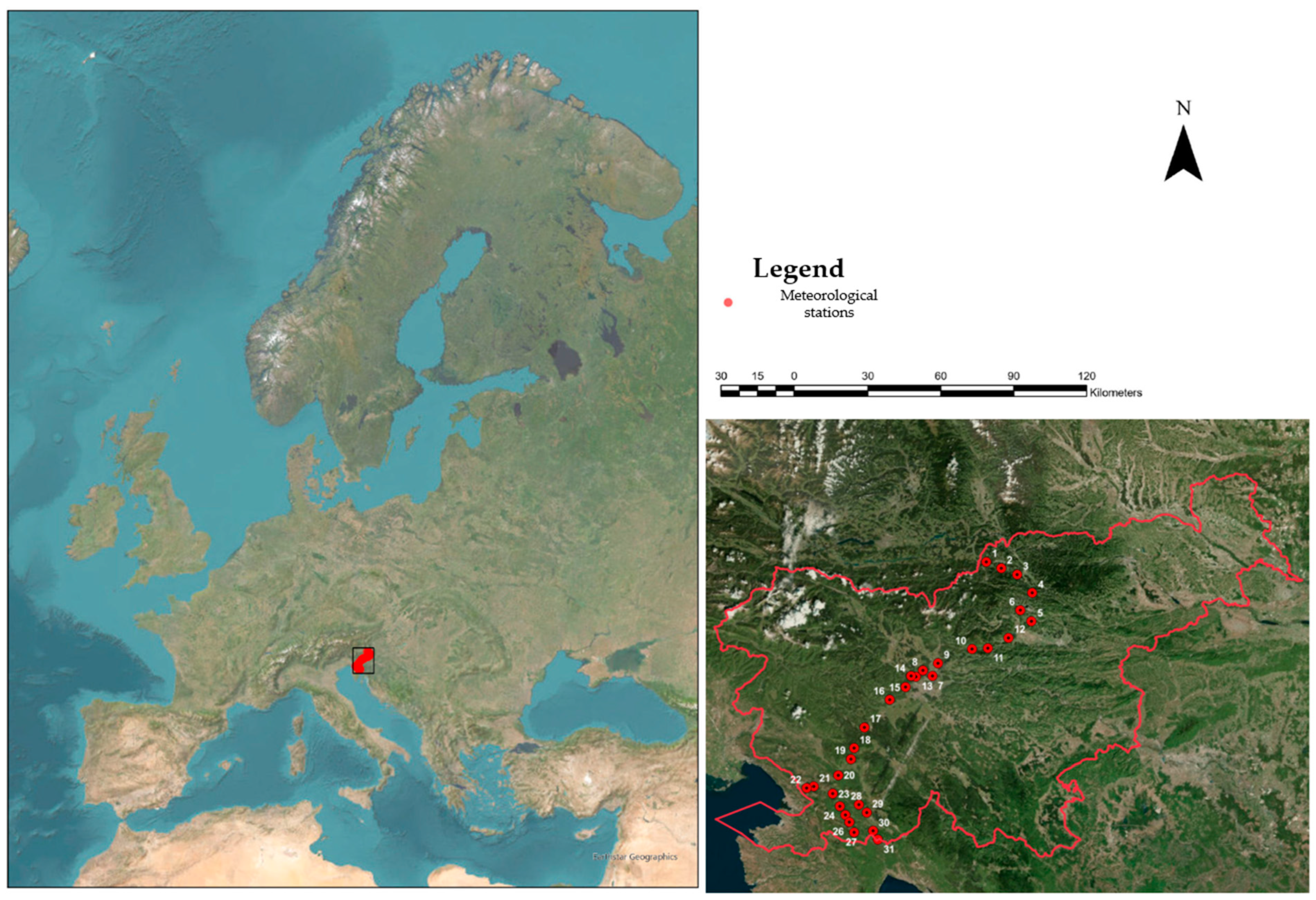
2.3. Meteorological Data from Measurement Stations (MAS)

Wind speed, temperature, and relative humidity were measured using the Vaisala WXT 536 device, while solar radiation data were recorded with the Kipp & Zonen SMP6 sensor. Meteorological sensors were mounted on power line poles 10 m above ground level. Measurement quality was ensured by the following:

• Routine maintenance of the equipment;
• Regular calibrations to uphold accuracy;
• Maintaining traceability for all measurement-related activities.

The data, owned by ELES, d.o.o., the operator of the Republic of Slovenia’s combined transmission and distribution power network, were utilized with their permission. The measurement locations are illustrated in Figure 1. Detailed information about station distribution, elevation, and land use is provided in Supplementary Material, Table S1.

2.4. Calculation of Combined Measurement Uncertainty

To calculate the combined measurement uncertainty for each meteorological parameter, this study followed a structured process: (i) identification of sources: identification of all sources contributing to uncertainty and determined their probability distributions; (ii) quantification: the magnitudes of each uncertainty contribution were calculated or determined; (iii) inter-correlation analysis: the relationships between influential quantities were analyzed; and (iv) standardization: to ensure consistency in the confidence level of all contributions, each uncertainty was converted into a standard measurement uncertainty.

The combined measurement uncertainty comprises uncertainties arising from the measurement equipment, its installation, systematic error (u_BIAS), and deviations (u_RT), which result from discrepancies between the model estimates and measured values. The uncertainty associated with the measurement equipment includes multiple components that differ depending on the parameter being measured. These contributions are summarized based on the manufacturer’s specifications and certificates.

Measurement uncertainties resulting from individual deviations (u_RT) and systematic differences (u_BIAS) were determined by comparing the measured values from meteorological stations at specific locations with the model-derived values calculated using the third method. Both types of uncertainty consider the temporal synchronization of the data and the measurement location, with the measured values serving as the reference. The forecasted model values, referred to as generated wind data (GWD), represent the model-derived estimates of the meteorological parameters using the third method. To determine u_RT and u_BIAS, it was assumed that the relationship between the measured values from the meteorological stations and the model-derived values could be expressed through a linear equation (Equation (1)) [44]:

$$y_i=\mathrm{a}+\mathrm{b}{x}_i$$

(1)

In this equation, a and b are the coefficients of the linear function, y_i represents the model-derived results, and x_i denotes the measured values. In the linear relationship between two variables, the method of least squares is typically used to determine the best linear fit and calculate the measurement uncertainty [44]. However, in cases like ours, where the values measured at meteorological stations are also subject to measurement errors, a specialized version of the least squares method, known as orthogonal regression, is more appropriate. Orthogonal regression accounts for errors in both variables (measured and model-derived), leading to a more accurate fit and better estimation of measurement uncertainty [45,46] making it particularly useful for assessing uncertainty in meteorological measurements.

However, this approach has certain limitations. One key assumption of orthogonal regression is that measurement errors are normally distributed and have constant variance (homoscedasticity). In reality, meteorological data often exhibit heteroskedasticity. meaning that the measurement errors vary across different data ranges. Since orthogonal regression does not always account for this variability, uncertainty estimates may be less reliable for datasets where measurement errors increase or decrease with the magnitude of the observed values [47].

Despite these limitations, orthogonal regression remains a suitable method in this study, as it provides a more realistic representation of measurement uncertainty compared to the ordinary least squares approach, particularly when both the measured and modelled values contain inherent errors.

2.5. Uncertainty of Deviation Resulting from Individual Measurements

Measurement uncertainty, brought by deviations of individual measurements of u_RT, is calculated using Equation (2) [43,44,46]:

$${\mathrm{u}}_{RT}^2\left(y_i\right)={\displaystyle \frac{RSS}{\left(n-2\right)}}+{[\mathrm{a}+\left(\mathrm{b}-1\right)x_i]}^2$$

(2)

where $u_{RT}\left(y_i\right)$ represents the uncertainty of the GWD results, RSS is the sum of the residuals arising from orthogonal regression, n is the number of samples, x_i are the measured values from the meteorological station, and a and b are the coefficients of the linear function. The RSS arising from orthogonal regression is calculated using Equation (3) [43,44,46]:

$$RSS={\sum }_{i=1}^n{\left(y_i-a-b{x}_i\right)}^2$$

(3)

The algorithm used to calculate the parameters a and b for orthogonal regression is expressed in formulas from Equation (4) to (10) [43,44,46]:

Calculation of the Slope b (Equation (4)):

$$b={\displaystyle \frac{S_{yy}-S_{xx}+\sqrt{{(S_{yy}-S_{xx)}}^2+4{\left(S_{xy}\right)}^2}}{2S_{xy}}}$$

(4)

where x_i is the value measured by meteorological stations, and y_i is the modelled value obtained from GWD [43]:

$$S_{xx}={\sum }_{i=1}^{N_{ux}}{\left(x_i-\overline{x}\right)}^{2}b$$

(5)

$$S_{yy}={\sum }_{i=1}^{N_{ux}}{\left(y_i-\overline{y}\right)}^2$$

(6)

$$S_{xy}={\sum }_{i=1}^{N_{ux}}\left(x_i-\overline{x}\right)\left(y_i-\overline{y}\right)$$

(7)

$$\overline{x}={\displaystyle \frac{\sum _{i=1}^{N_{ux}}{x}_i}{N_{ux}}}$$

(8)

$$\overline{y}={\displaystyle \frac{\sum _{i=1}^{N_{ux}}{y}_i}{n}}$$

(9)

Calculation of the initial value a (Equation (10)):

$$\mathrm{a}=\overline{y}-b\overline{x}$$

(10)

2.6. Uncertainty BIAS

BIAS uncertainty refers to the uncertainty associated with the systems or method’s deviation from the reference value. BIAS results from systematic errors that lead to systematic deviations of the results from the true value.

BIAS uncertainty is calculated based on Equation (11):

$$u_{BIAS}\left(y\right)=a+\left(b-1\right)MV$$

(11)

In Equation (11), a and b represent the initial value and the slope obtained through orthogonal regression. MV represents the value of the individual parameter. BIAS uncertainty depends on the actual value of the measured or predicted parameter and varies accordingly.

For the parameters, such as temperature, wind speed, relative humidity, and solar radiation, the combined measurement uncertainty for the predicted model values of GWD has been calculated. Contributions to the measurement uncertainty are listed below and separated for each influencing parameter [43,44,46].

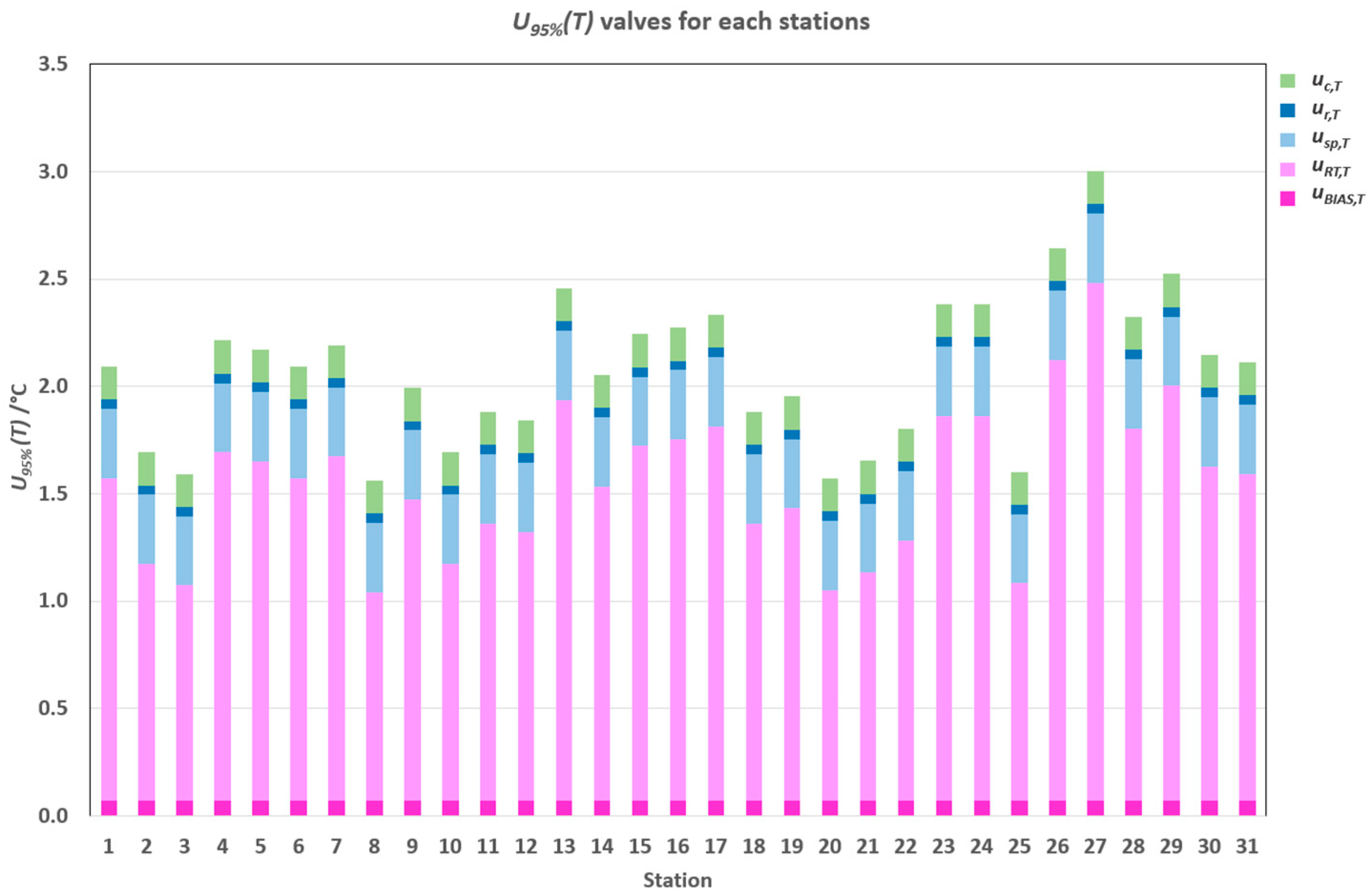
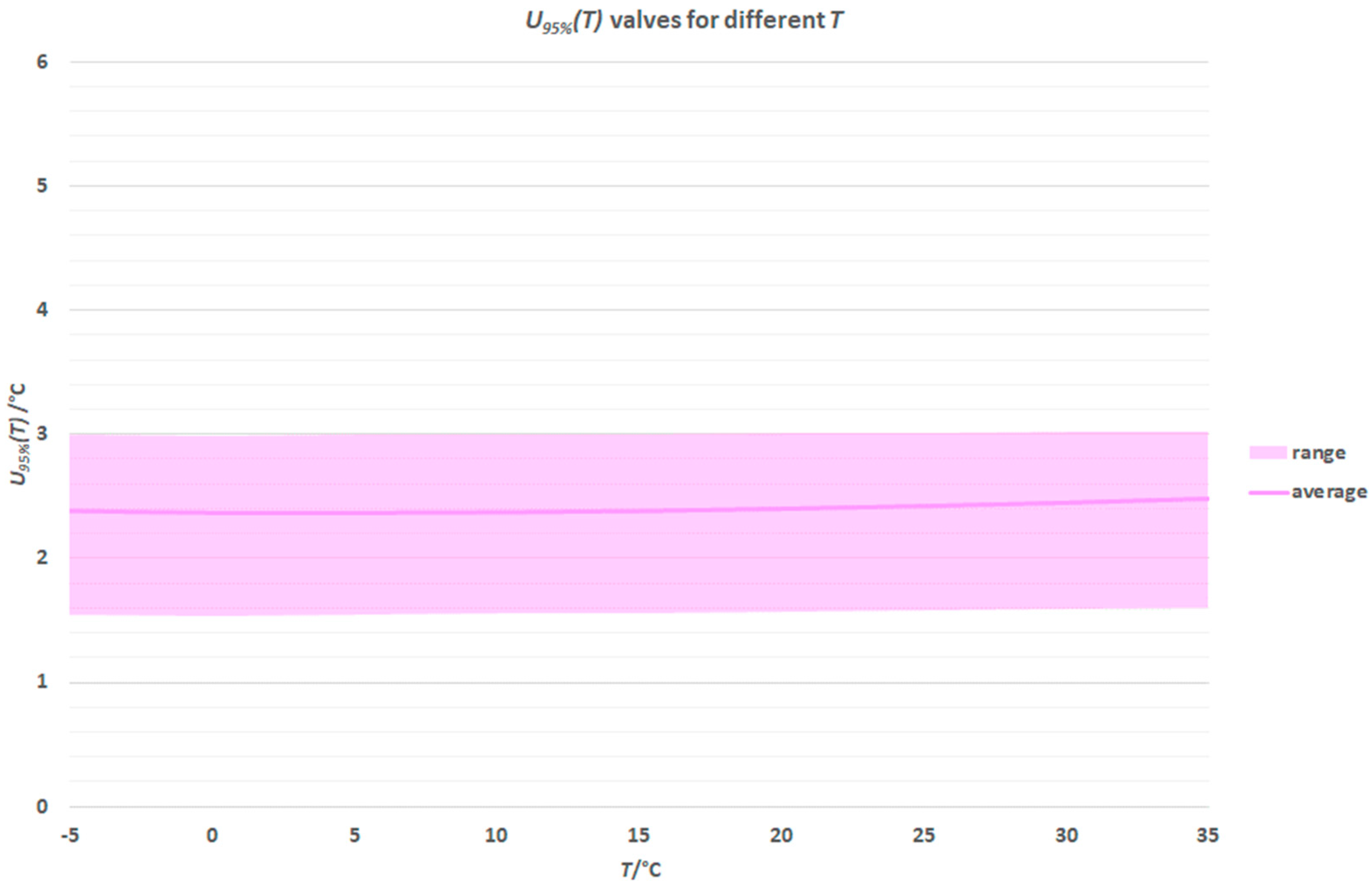
2.7. Temperature Measurement Uncertainty

The combined measurement uncertainty of temperature, u_c(T), consists of contributions from various sources, including measurement equipment, calibration processes, and differences between the meteorological measurements and the predicted values from GWD. The contributions arising from the measurement equipment are summarized based on the manufacturer’s specifications. The u_c(T) is calculated using Equation (12) and includes the following contributions:

• uncertainty of accuracy from the reference method (u_sp,T);
• uncertainty of resolution from the reference method (u_r,T);
• calibration uncertainties of the reference method (u_c,T);
• uncertainty based on systematic difference (BIAS) (u_BIAS,T);
• uncertainties due to deviations in GWD (u_RT,T).

When determining the measurement uncertainty of the temperature obtained from model estimates, there is no correlation between individual quantities. Therefore, the sensitivity coefficient c_T is equal to one [43,44,46]:

$$u_c\left(T\right)=\sqrt{{c_{\mathrm{T}}^2(u}_{sp,T}^2+u_{r,,T}^2+u_{c,T}^2+u_{BIAS,T}^2+u_{RT,T}^2)}$$

(12)

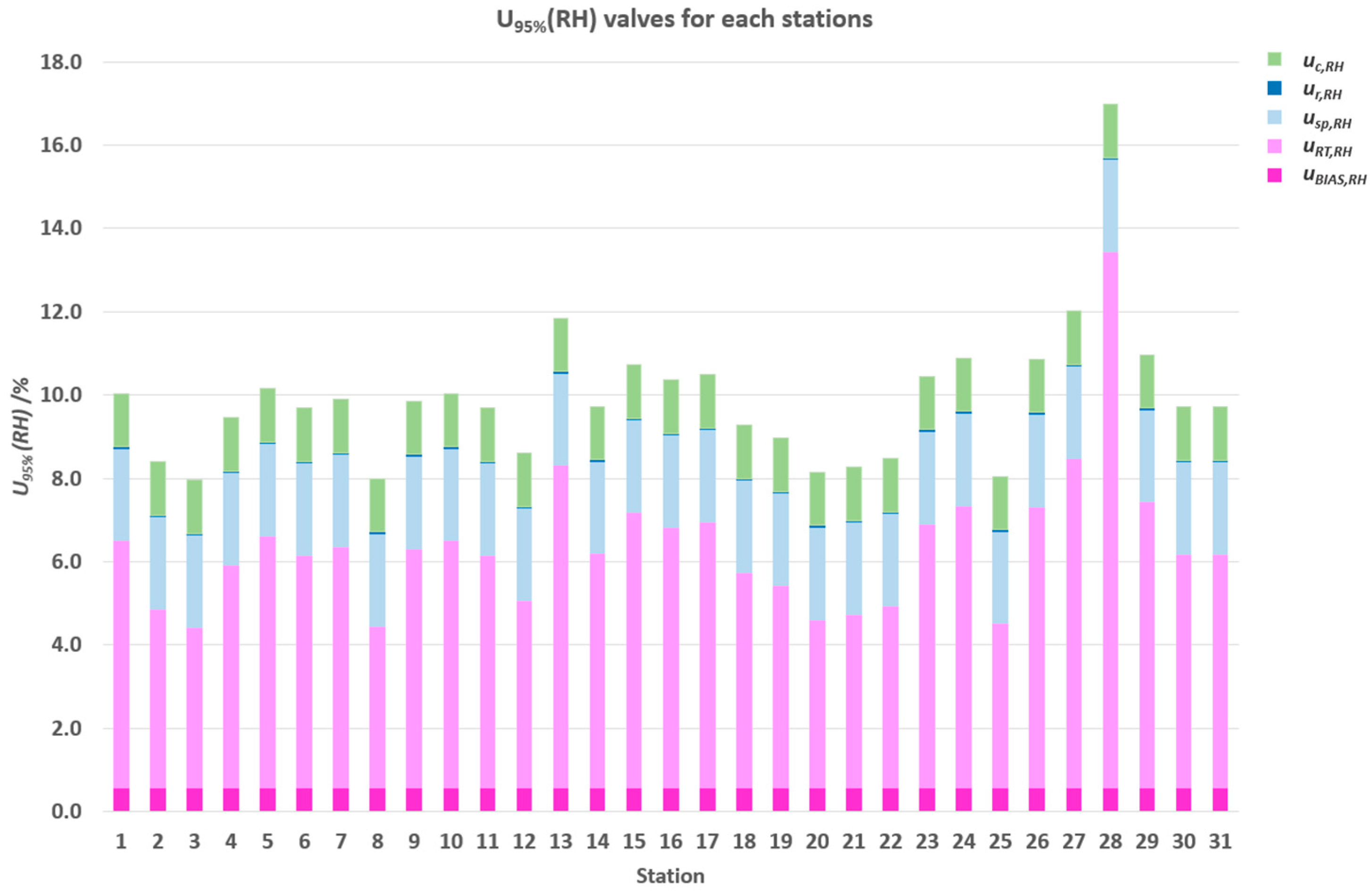
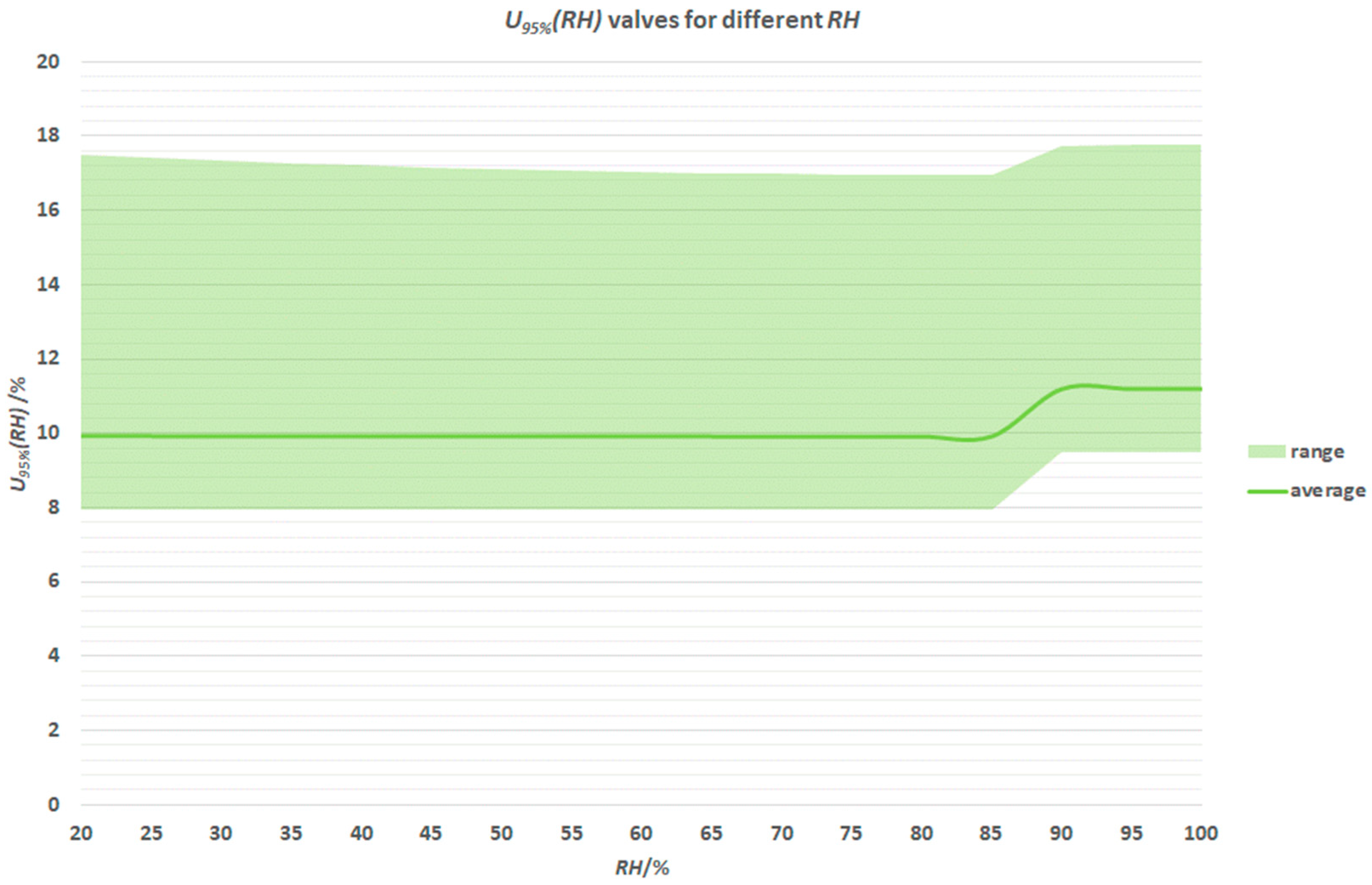
2.8. Relative Humidity Measurement Uncertainty

The combined measurement uncertainty of relative humidity, u_c(RH), is composed of contributions arising from the measurement equipment, summarized based on the manufacturer’s specifications, calibrations, and uncertainties resulting from differences between the meteorological measurements and the predicted values from GWD. The u_c(RH) is calculated using Equation (13) and includes the following contributions [43,44,46]:

• uncertainty of accuracy from the reference method (u_sp,RH);
• uncertainty of resolution from the reference method (u_r,RH);
• calibration uncertainties of the reference method (u_c,RH);
• uncertainty based on systematic difference (BIAS) (u_BIAS,RH);
• uncertainties due to deviations in GWD (u_RT,RH).

$$u_c\left(RH\right)=\sqrt{{c_{\mathrm{R}\mathrm{H}}^2(u}_{sp,\mathrm{R}\mathrm{H}}^2+u_{r,\mathrm{R}\mathrm{H}}^2+u_{c,\mathrm{R}\mathrm{H}}^2+u_{BIAS,\mathrm{R}\mathrm{H}}^2+u_{RT,\mathrm{R}\mathrm{H}}^2)}$$

(13)

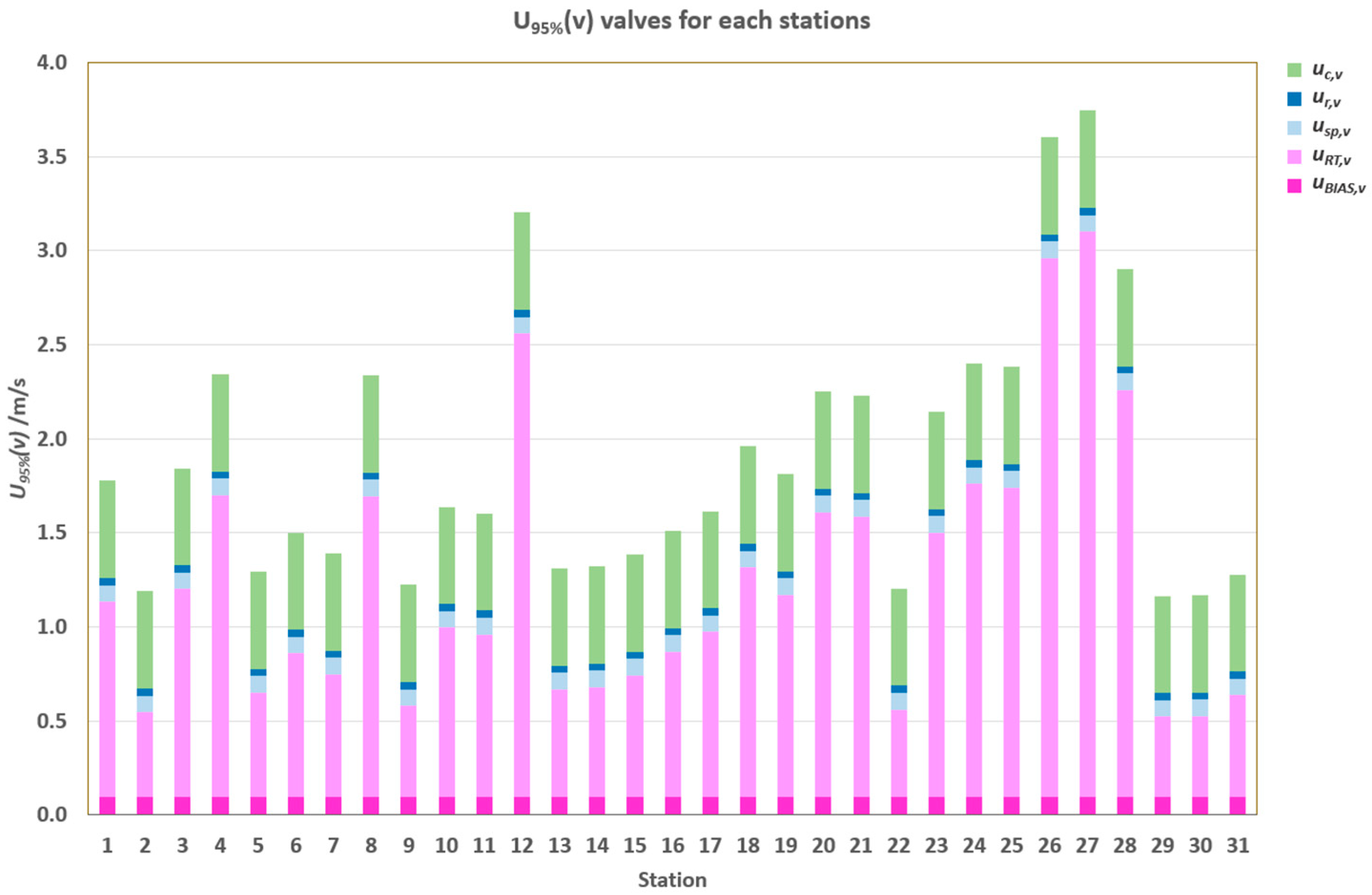
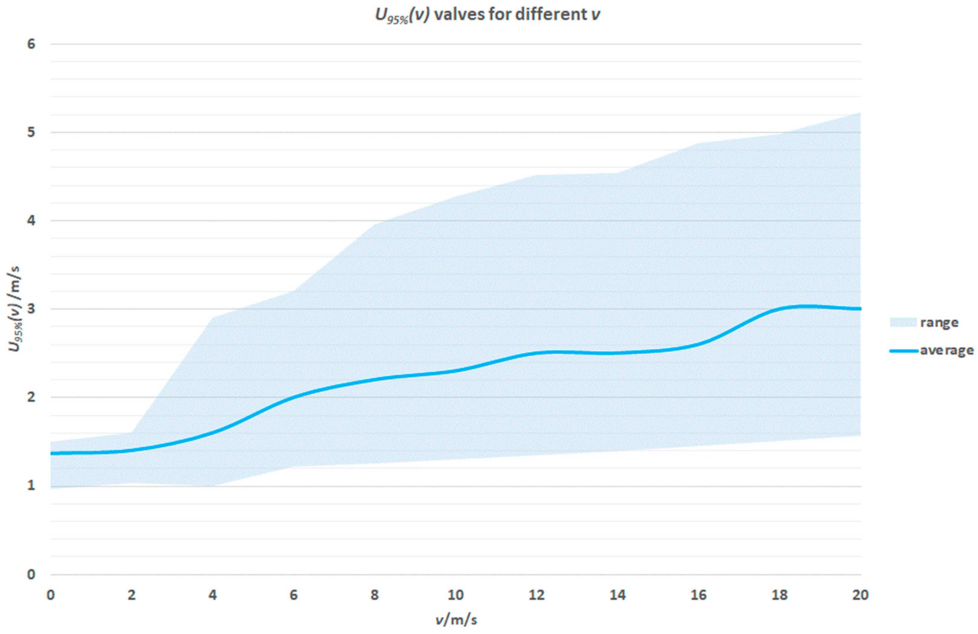
2.9. Measurement Uncertainty of Wind Speed

The combined measurement uncertainty for wind speed, u_c(v), consists of contributions from various sources, including the measurement equipment, calibration processes, and differences between the meteorological measurements and the predicted values from GWD. The contributions arising from the measurement equipment are summarized based on the manufacturer’s specifications. The combined measurement uncertainty for wind speed is calculated using Equation (14) and includes the following components [43,44,46]:

• uncertainty of accuracy from the reference method (u_sp,v);
• uncertainty of resolution from the reference method (u_r,v);
• calibration uncertainties of the reference method (u_c,v);
• uncertainty based on systematic differences (BIAS) (u_BIAS,v);
• uncertainties due to deviations in GWD (u_RT,v)

$$u_c\left(v\right)=\sqrt{{c_v^2(u}_{sp,\mathrm{v}}^2+u_{r,\mathrm{v}}^2+u_{c,\mathrm{v}}^2+u_{BIAS,\mathrm{v}}^2+u_{RT,\mathrm{v}}^2)}$$

(14)

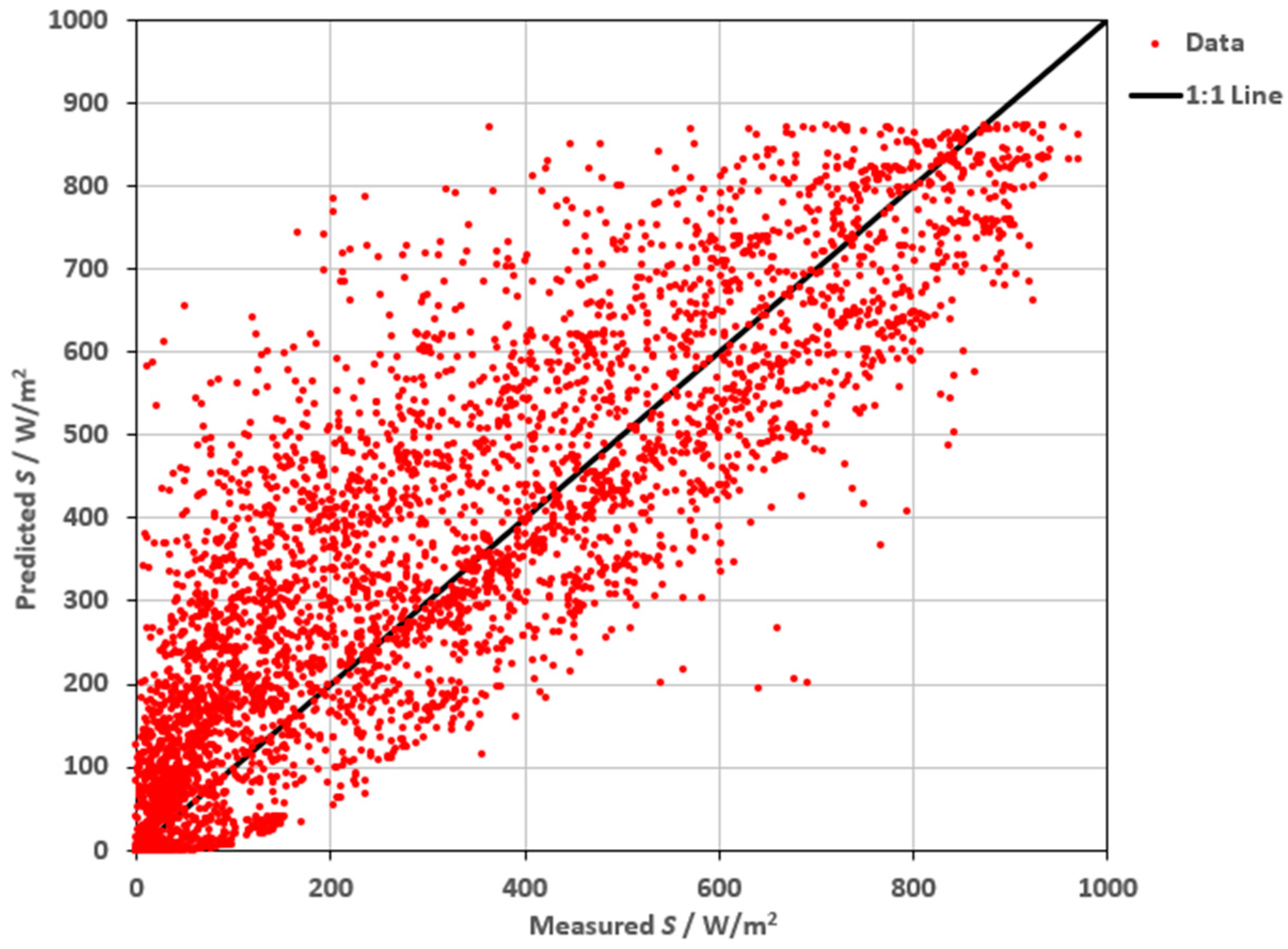
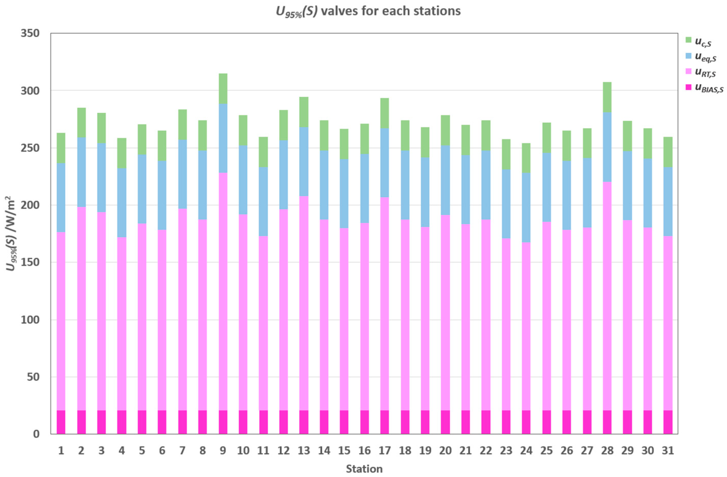
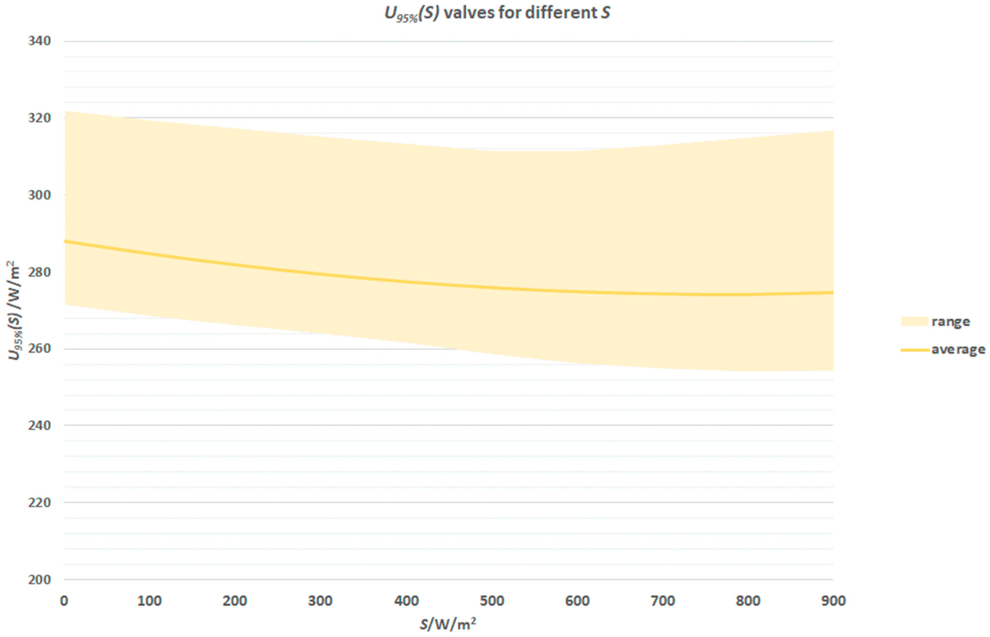
2.10. Measurement Uncertainty of Solar Radiation

The combined measurement uncertainty of solar radiation, u_c(S), is composed of contributions arising from the measurement equipment, summarized according to the manufacturer’s specifications, calibrations, and uncertainties resulting from differences between the meteorological measurements and the predicted values (GWD). The u_c(S) is calculated using Equation (15) and includes the following contributions [43,44,46]:

• uncertainty due to zero offset of the reference method (u_ZERO,S);
• uncertainty due to drift of the reference method (u_D,S);
• uncertainty due to nonlinearity of the reference method (u_L,S);
• uncertainty due to temperature response of the reference method (u_T,S);
• uncertainty due to the angle of incidence of the sun (u_S,S);
• uncertainty due to spectral selectivity of the reference method (u_ss,S);
• uncertainty due to the tilt of the reference method (u_TR,S);
• uncertainty due to resolution of the reference method (u_r,S);
• calibration uncertainties of the reference method (u_c,S);
• uncertainty based on systematic difference (BIAS) (u_BIAS,S);
• uncertainties due to deviations in GWD (u_RT,S).

$$u_c\left(v\right)=\sqrt{\begin{array}{c}{c_{\mathrm{S}}^2(u_{ZERO,\mathrm{S}}^2+u_{L,\mathrm{S}}^2+u_{T,\mathrm{S}}^2+u_{S,\mathrm{S}}^2+u}_{ss,\mathrm{S}}^2\\ +u_{TR,\mathrm{S}}^2+u_{r,\mathrm{S}}^2+u_{c,\mathrm{S}}^2+u_{BIAS,\mathrm{v}}^2+u_{RT,\mathrm{v}}^2)\end{array}}$$

(15)

2.11. Probability Distributions of Individual Contributions

Uncertainty due to the resolution of the measuring instrument, denoted as u_r,T, u_r,RH, u_r,_v, and u_r,S, is considered for all of the meteorological parameters and is summarized according to the specifications of the measurement equipment [48]. The uncertainty of resolution is provided with both a lower and upper limit, and due to its contribution, it needs to be divided by $\sqrt{12}$. Other contributions, also summarized from the specifications of the measurement equipment, such as u_sp,T, u_sp,RH, u_sp,v, u_ZERO,S, u_S,S, u_D,S, u_L,S, u_T,S, u_ss,S u_TR,S, are distributed according to a rectangular probability distribution and need to be divided by $\sqrt{3}.$

Calibration uncertainty, denoted as u_c,T, u_c,RH, u_c,v, in u_c,S, is summarized from the calibration certificate [48,49] which indicates a normal distribution (expanded measurement uncertainty k = 2). This contribution should be divided by 2.

The standard uncertainties of systematic error BIAS u_BIAS,T, u_BIAS,RH, u_BIAS,v, or u_BIAS,S, and the uncertainties resulting from deviations of individual measurements, u_RT,T, u_RT,RH, u_RT,v or u_RT,S, are calculated using Equations (2) and (11).

The calculated combined standard measurement uncertainty for each parameter provides a result with a 68.3% confidence level. However, to achieve a higher confidence level, at least 95%, the obtained results are multiplied by a factor of k = 2, as shown in Equation (15):

$$U_{\left(95\%\right)} \left(y\right)=k·u_c\left(y\right)$$

(16)

3. Results and Discussion

The calculated expanded measurement uncertainty, with a confidence interval of 95.5%, is derived from the annual dataset for 2022. The results of the expanded measurement uncertainty for each meteorological parameter, as determined using the microscale meteorological model CALMET and incorporating data from meteorological stations, are illustrated in the figures below.

3.1. Temperature

The relationship between the measured and predicted temperature values provides insights into the reliability of the model predictions. Figure 2 illustrates this relationship for station 6, located in a wide grassland area. At this location, the relationship between the measured values obtained from the meteorological station and the predicted GWD values is very stable and follows an almost perfect linear correlation. This indicates a good agreement between the model predictions and the measured values.

Figure 3 shows the expanded measurement uncertainty for temperature (U_95%(T)) at 15 °C across each meteorological station, with the contributions of the individual uncertainty components clearly distinguished. They are provided proportionally according to their contribution. These components include calibration uncertainty (u_c,T), resolution uncertainty (u_sp,T), accuracy uncertainty of the method (u_sp,T), systematic differences (u_BIAS,T), and deviations of individual measurements (u_RT,T). The graph reveals that the largest contribution to the expanded measurement uncertainty for temperature arises from deviations between the measured and predicted values (u_RT,T), while other components have a smaller influence. Differences between stations are attributed to local factors, with higher uncertainties observed at stations 26, 27, and 29, located near forested areas. These influences may be related to the direct impact of trees on the temperature measurements or an improper placement of the measurement equipment in shaded or highly sunlit areas.

Figure 4 illustrates the measurement uncertainty for temperature across the entire measured area. The line on the graph represents the average measurement uncertainty for temperature, calculated based on the uncertainties at all stations. The shaded area on the chart indicates the minimum and maximum measurement uncertainties corresponding to individual temperature values. This visualization provides a clearer understanding of the variability in uncertainty across different temperature ranges [27].

3.2. Relative Humidity

The relationship between the measured and predicted relative humidity values provides insight into the reliability of model predictions. Figure 5 illustrates this relationship for meteorological station 6, where a good agreement between measured and predicted values can be observed. The 1:1 line in the graph indicates a perfect match between the measured and predicted values, while the red dots represent the dispersion of the actual data points. The results show a stable relationship between the measured and predicted values in most cases. However, a slight deviation is noticeable at higher relative humidity values.

Figure 6 presents the expanded measurement uncertainty for relative humidity (U_95%(RH)) at 80% RH for each meteorological station, with individual components of measurement uncertainty clearly distinguished. They are provided proportionally according to their contribution. The main contribution to the overall uncertainty comes from deviations in individual measurements (u_RT,RH).

The relative humidity measurements showed uncertainties ranging from 8% to 12% RH, with the exception of station 28, located in a forested area. The significantly higher uncertainty at this station was traced to a malfunctioning capacitive humidity sensor. After replacing the sensor at the end of 2022, discrepancies between the measured and predicted values were significantly reduced.

The measurement uncertainty for relative humidity across the entire measured area is depicted in Figure 7 [27]. The shaded area represents the range of minimum and maximum uncertainties for individual relative humidity values, while the line indicates the average uncertainty calculated across all stations. This visualization provides a better insight into the variability of relative humidity uncertainty across the entire measured area.

3.3. Wind Speed

The relationship between the measured and predicted wind speed values is shown in Figure 8, providing insight into the agreement between the model predictions and measured values at station 6. The 1:1 line indicates a perfect match between measured and predicted values, while the red dots represent the actual data points.

Figure 9 presents the expanded measurement uncertainty U_95%(v) for wind speed at 4 m/s across each meteorological station, with individual components of measurement uncertainty clearly delineated. They are provided proportionally according to their contribution. The main contribution to the overall uncertainty arises from deviations between the measured and predicted values (u_RT,v).

Wind speed uncertainty depends on the actual measured value and increases with higher wind speeds. At lower wind speeds, the uncertainty ranges between 1 and 2 m/s, whereas at higher wind speeds, it averages above 3 m/s. This dependency is clearly evident in Figure 9, where the stations with higher average wind speeds exhibit correspondingly higher measurement uncertainties. The largest uncertainties are observed at stations 26 and 27, which are exposed to more extreme weather conditions and higher average wind speeds.

The average measurement uncertainty of wind speed, along with the range of minimum and maximum values, is shown as the shaded area in Figure 10 [27]. This analysis confirms the need for improvements in the models that can more accurately predict conditions at higher wind speeds, as well as a further evaluation of local factors influencing wind dynamics.

3.4. Solar Radiation

The relationship between the measured and predicted solar radiation values for location 6, situated in an open area with minimal local influences, is shown in Figure 11. The 1:1 line represents the reference for a perfect match between the measured and predicted values, while the red dots depict the actual data points. Deviations are evident at higher solar radiation values, where the measured values in full sunlight reach up to 1200 W/m². Meanwhile, the highest predicted values are capped at 900 W/m². This discrepancy highlights the need for a systematic data analysis approach to reduce uncertainty, particularly at higher solar radiation values.

Figure 12 illustrates the expanded measurement uncertainty (U_95%(S)) for solar radiation at 800 W/m². Contributions originating from the specifications of the measurement equipment are combined into a single overall contribution (u_eq,S), which constitutes a significant part of the total uncertainty. The sum of (u_eq,S) includes contributions from various factors, such as u_ZERO,S, u_D,S, u_L,S, u_T,S, u_S,S, u_ss,S, u_TR,S, and u_r,S. The primary contribution to the total uncertainty arises from deviations between the measured and predicted values (u_RT,S). These uncertainties vary between stations, with local factors, such as changes in the angle of solar radiation and specific microclimatic conditions, playing a key role in influencing variability in uncertainty. Figure 12 illustrates the calculated uncertainty for each meteorological station, clearly revealing the differences between various locations.

Figure 13 provides an overview of the measurement uncertainty across the entire measured area. The line on the graph represents the average uncertainty for solar radiation, derived from the uncertainties at all stations. The shaded area on the chart highlights the range between the minimum and maximum uncertainties for the individual solar radiation values [27].

For solar radiation, high measurement uncertainty is due to the discrepancy between the measured and predicted values. Measured solar radiation peaks were at 1200 W/m², but the model limits forecasts to 900 W/m², suggesting potential underestimation. This difference highlights the need for a systematic approach to data analysis to minimize uncertainty.

3.5. Practical Implications of Findings

The findings of this study have significant practical implications for industries that rely on accurate meteorological data. particularly in energy transmission, agriculture, and disaster management.

• For energy transmission, accurate meteorological forecasts are critical for assessing transmission efficiency and optimizing the operation of high-voltage power lines. Temperature and wind speed directly influence line sagging and energy losses, while solar radiation data contribute to the integration of renewable energy sources into the grid. Reducing measurement uncertainty enhances grid stability and energy distribution reliability;
• For agriculture, meteorological models are widely used in crop management, irrigation planning, and extreme weather prediction. The reduction of uncertainty in temperature and solar radiation forecasts allows for better decision-making in planting schedules, pest control, and yield optimization, particularly in regions with high climatic variability;
• For disaster management, reliable meteorological models are essential for early-warning systems and risk mitigation strategies. Improved accuracy in wind speed and humidity predictions contributes to better wildfire risk assessments, while enhanced temperature and precipitation estimates support flood forecasting and drought monitoring.

These findings indicate that the CALMET model, with improved uncertainty quantification, can provide more reliable meteorological inputs for decision-making in various sectors. Future enhancements in model integration, including better incorporation of local topographic effects and land-use variability, could further refine its applications.

4. Conclusions

This study is focused on evaluating the measurement uncertainty of meteorological parameters calculated using the diagnostic microscale meteorological model CALMET. It is believed that this study has demonstrated that measurement uncertainty plays a critical role in meteorological forecasting, particularly in the context of energy transmission in Slovenia. The key findings emphasize that measurement uncertainty, particularly for temperature, relative humidity, solar radiation, and wind speed, significantly influences the reliability of meteorological predictions. While fluctuations in uncertainty are minimal across stations, local factors and limitations in measurement equipment introduce variability, which must be addressed to ensure the quality of forecasts.

Also, the analysis of the data and graphs derived from the CALMET model underscores the critical importance of addressing measurement uncertainty when interpreting meteorological parameters. The practical applications of these findings are evident in the energy sector, where accurate weather forecasts are essential for predicting the flow of electricity through powerlines. By improving the accuracy of forecasts, particularly for wind speed and solar radiation, energy distributors in Slovenia can optimize the transmission of electricity, reducing the risks of overloading power grids or insufficient energy generation. Furthermore, these improvements can enhance the management of natural resources, disaster response efforts, and the optimization of agricultural and industrial processes that rely on precise weather data.

Although this study provides valuable insights into measurement uncertainty, certain limitations must be acknowledged. The analysis is based on a single year of data, which may not capture long-term variations in meteorological conditions. Expanding the study to multi-year datasets would allow for a more comprehensive assessment of uncertainty trends over time. The model does not fully account for all local factors, such as small-scale land-use changes, vegetation dynamics, and urban heat island effects, which may introduce additional uncertainties. To reduce measurement uncertainty, several specific actions should be taken. (i) Improve the measurement equipment, particularly for parameters like relative humidity, where the uncertainty increases above 85%. Upgrading sensors and calibration methods would lead to more precise data collection. (ii) Refine the CALMET model to integrate local factors, such as land-use changes, vegetation dynamics, and urban heat islands, which have a significant impact on the accuracy of meteorological predictions. (iii) Integrate additional data sources, such as real-time satellite observations and ground-based sensors, to enhance the model’s predictive accuracy and reduce uncertainty in forecasting.

This study, therefore, highlights the importance of addressing measurement uncertainty to improve the accuracy and reliability of weather forecasts. It emphasizes that refining the meteorological models and measurement systems can contribute to better decision-making processes in various sectors, particularly in energy transmission. Future research should explore advanced statistical correction methods and hybrid modeling approaches to reduce uncertainty in CALMET-derived forecasts. By advancing measurement techniques and integrating diverse data sources, meteorological forecasting will continue to improve, supporting better planning, risk management, and resource optimization.

References

1. Jain, H.; Dhupper, R.; Shrivastava, A.; Kumar, D.; Kumari, M. Leveraging machine learning algorithms for improved disaster preparedness and response through accurate weather pattern and natural disaster prediction. Front. Environ. Sci. 2023, 11, 1–14. [Google Scholar] [CrossRef]
2. Collins, B.; Lai, Y.; Grewer, U.; Attard, S.; Sexton, J.; Pembleton, K.G. Evaluating the impact of weather forecasts on productivity and environmental footprint of irrigated maize production systems. Sci. Total Environ. 2024, 954, 176368. [Google Scholar] [CrossRef] [PubMed]
3. Županić, F.Ž.; Radić, D.; Podbregar, I. Climate change and agriculture management: Western Balkan region analysis. Energy Sustain. Soc. 2021, 11, 1–9. [Google Scholar] [CrossRef]
4. Park, H.; Chung, S. Utilization of a Lightweight 3D U-Net Model for Reducing Execution Time of Numerical Weather Prediction Models. Atmosphere 2025, 16, 60. [Google Scholar] [CrossRef]
5. Bogataj, L.K.; Sušnik, A. Challenges to Agrometeorological Risk Management—Regional Perspectives: Europe. In Managing Weather and Climate Risks in Agriculture; Springer: Berlin/Heidelberg, Germany, 2019; Volume 11. [Google Scholar]
6. EU MET SAT. 2025. Available online: https://www.eumetsat.int/ (accessed on 5 March 2025).
7. ECMWF. 2025. Available online: https://www.ecmwf.int/ (accessed on 5 March 2025).
8. ELES. 2025. Available online: https://www.eles.si/en (accessed on 5 March 2025).
9. Lei, M.; Shiyan, L.; Chuanwen, J.; Hongling, L.; Yan, Z. A review on the forecasting of wind speed and generated power. Renew. Sustain. Energy Rev. 2009, 13, 915–920. [Google Scholar] [CrossRef]
10. Kang, S.; Hadadi, S.; Yu, S.; Lee, S.-I.; Seo, D.-W.; Oh, J.; LeeWind, J.-H. resource assessment and potential development of wind farms along the entire coast of South Korea using public data from the Korea meteorological administration. J. Clean. Prod. 2023, 430, 139378. [Google Scholar] [CrossRef]
11. van der Meer, J.; Callier, M.; Fabi, G.; van Hoof, J.L.; Nielsen, R.; Raicevich, S. The carrying capacity of the seas and oceans for future sustainable food production: Current scientific knowledge gaps. Food Energy Secur. 2023, 12, e464. [Google Scholar] [CrossRef]
12. Mirás-Avalos, J.M.; Escalona, J.M.; Pérez-Álvarez, E.P.; Romero, P.; Botia, P.; Navarro, J.; Torres, N.; Santesteban, L.G.; Uriarte, D.; Intrigliolo, D.S.; et al. Upgrading and validating a soil water balance model to predict stem water potential in vineyards. Agric. For. Meteorol. 2024, 359, 110281. [Google Scholar] [CrossRef]
13. del Río, S.; Álvarez-Esteban, R.; Alonso-Redondo, R.; Álvarez, R.; Rodríguez-Fernández, M.P.; González-Pérez, A.; Penas, A. Applications of bioclimatology to assess effects of climate change on viticultural suitability in the DO León (Spain). Theor. Appl. Climatol. 2024, 155, 3387–3404. [Google Scholar] [CrossRef]
14. Jiang, Z.; Yang, S.; Liu, Z.; Xu, Y.; Xiong, Y.; Qi, S.; Pang, Q.; Xu, J.; Liu, F.; Xu, T. Coupling machine learning and weather forecast to predict farmland flood disaster: A case study in Yangtze River basin. Environ. Model. Softw. 2022, 155, 105436. [Google Scholar] [CrossRef]
15. Prieto, C.; Patel, D.; Han, D.; Dewals, B.; Bray, M.; Molinari, D. Preface: Advances in pluvial and fluvial flood forecasting and assessment and flood risk management. Nat. Hazards Earth Syst. Sci. 2024, 24, 3381–3386. [Google Scholar] [CrossRef]
16. Patriarca, R.; Simone, F.; Di Gravio, G. Supporting weather forecasting performance management at aerodromes through anomaly detection and hierarchical clustering. Expert Syst. Appl. 2023, 213, 119210. [Google Scholar] [CrossRef]
17. Lonati, G.; Cernuschi, S.; Giani, P. Air Quality Impact Assessment of a Waste-to-Energy Plant: Modelling Results vs. Monitored Data. Atmosphere 2022, 13, 516. [Google Scholar] [CrossRef]
18. Sówka, I.; Paciorek, M.; Skotak, K.; Kobus, D.; Zathey, M.; Klejnowski, K. The analysis of the effectiveness of implementing emission reduction measures in improving air quality and health of the residents of a selected area of the lower silesian voivodship. Energies 2020, 13, 4001. [Google Scholar] [CrossRef]
19. Pucer Strumbelj, J.F.E. Impact of changes in climate on air pollution in Slovenia between. Environ. Pollut. 2018, 242, 398–406. [Google Scholar] [CrossRef]
20. Wu, Y.; Xue, W. Data-Driven Weather Forecasting and Climate Modeling from the Perspective of Development. Atmosphere 2021, 15, 689. [Google Scholar] [CrossRef]
21. Moulin, A.; Benedetti, L.; Gosar, A.; Rupnik, P.J.; Rizza, M.; Bourlès, D.; Ritz, J.-F. Determining the present-day kinematics of the Idrija fault (Slovenia) from airborne LiDAR topography. Tectonophysics 2014, 628, 188–205. [Google Scholar] [CrossRef]
22. Stefanovski, S.; Kokalj, Ž.; Stepišnik, U. Sky-view factor enhanced doline delineation: A comparative methodological review based on case studies in Slovenia. Geomorphology 2024, 465, 109389. [Google Scholar] [CrossRef]
23. Tarraf, B.; Brun, F.; Raynaud, L.; Roux, S.; Zhang, Y.; Davadan, L.; Deudon, O. Assessing the impact of weather forecast uncertainties in crop water stress model predictions. Agric. For. Meteorol. 2024, 349, 109934. [Google Scholar] [CrossRef]
24. Tian, Y.; Jia, B.; Zhao, P.; Song, D.; Huang, F.; Feng, Y. Size distribution, meteorological influence and uncertainty for source-specific risks: PM2.5 and PM10-bound PAHs and heavy metals in a Chinese megacity during 2011–2021. Environ. Pollut. 2022, 312, 120004. [Google Scholar] [CrossRef]
25. Jian, L.; Yuze, S.; Huamei, W.; Xiangnan, W.; Kuan, L.; Hongming, Q. Study on measurement uncertainty of energy conversion efficiency of tidal energy converters. Energy Rep. 2024, 12, 4883–4890. [Google Scholar] [CrossRef]
26. Lei, X.; Lin, P.; Zheng, H.; Fei, W.; Yin, Z.; Ren, H. Systematic analyses of the meteorological forcing and process parameterization uncertainties in modeling runoff with Noah-MP for the Upper Brahmaputra river basin. J. Hydrol. 2024, 653, 132686. [Google Scholar] [CrossRef]
27. Bell, S. A Beginner’s Guide to Uncertainty of Measurement Measurement Good Practice Guide; National Physical Laboratory: Middlesex, UK, 1999. [Google Scholar]
28. Holnicki, P. Uncertainty in Integrated Modelling of Air Quality. In Advanced Air Pollution; InTech: Rijeka, Croatia, 2011. [Google Scholar]
29. Merlone, A.; Lopardo, G.; Sanna, F.; Bell, S.; Benyon, R.; Bergerud, R.A.; Bertiglia, F.; Bojkovski, J.; Böse, N.; Brunet, M.; et al. The MeteoMet Project—Metrology for meteorology: Challenges and results. Meteorol. Appl. 2015, 22, 820–829. [Google Scholar] [CrossRef]
30. Gómez-Navarro, J.J.; Raible, C.C.; Dierer, S. Sensitivity of the WRF model to PBL parametrisations and nesting techniques: Evaluation of wind storms over complex terrain. Geosci. Model Dev. 2015, 8, 3349–3363. [Google Scholar] [CrossRef]
31. Ortiz, P.; Casas, E.; Orescanin, M.; Powell, W.S.; Petkovic, V.; Hall, M. Uncertainty Calibration of Passive Microwave Brightness Temperatures Predicted by Bayesian Deep Learning Models. Artif. Intell. Earth Syst. 2023, 2. [Google Scholar] [CrossRef]
32. Morales, L.; Lang, F.; Mattar, C. Mesoscale wind speed simulation using CALMET model and reanalysis information: An application to wind potential. Renew. Energy 2012, 48, 57–71. [Google Scholar] [CrossRef]
33. González, A.J.; Hernández-Garcés, A.; Rodríguez, A.; Saavedra, S.; Casares, J.J. Surface and upper-Air WRF-CALMET simulations assessment over a coastal and complex terrain area. Int. J. Environ. Pollut. 2015, 57, 249–260. [Google Scholar] [CrossRef]
34. Ruggeri, F.M.; Lana, B.N.; Altamirano, C.J.; Puliafito, E.S. Spatial distribution, patterns and source contributions of POPs in the atmosphere of Great Mendoza using the WRF/CALMET/CALPUFF modelling system. Emerg. Contam. 2020, 6, 103–113. [Google Scholar] [CrossRef]
35. Tagliaferri, F.; Facagni, L.; Invernizzi, M.; Ferrer Hernández, A.L.; Hernández-Garces, A.; Sironi, S. Odor Impact Assessment via Dispersion Model: Comparison of Different Input Meteorological Datasets. Appl. Sci. 2024, 14, 2457. [Google Scholar] [CrossRef]
36. Oleniacz, R.; Rzeszutek, M. Intercomparison of the CALMET/CALPUFF modeling system for selected horizontal grid resolutions at a local scale: A case study of the MSWI Plant in Krakow, Poland. Appl. Sci. 2018, 8, 2301. [Google Scholar] [CrossRef]
37. Arregocés, A.H.; Rojano, R.; Restrepo, G. Effects of lockdown due to the covid-19 pandemic on air quality at Latin America’s largest open-pit coal mine. Aerosol Air Qual. Res. 2021, 21, 1–14. [Google Scholar] [CrossRef]
38. Indumati, S.; Oza, B.R.; Mayya, S.Y.; Puranik, D.V.; Kushwaha, S.H. Dispersion of pollutants over land-water-land interface: Study using CALPUFF model. Atmos. Environ. 2009, 43, 473–478. [Google Scholar] [CrossRef]
39. Scire, J.S.; Robe, F.R.; Fernau, M.E.; Yamartino, R.J. A User’s Guide for the CALMET Meteorological Model; Earth Tech, Inc.: Pasadena, CA, USA, 2000. [Google Scholar]
40. CALMET SRC. 2025. Available online: https://www.src.com/ (accessed on 5 March 2025).
41. CALPUFF. 2025. Available online: https://calpuff.org/ (accessed on 5 March 2025).
42. CALMET. 2025. Available online: https://www.enviroware.com/calmet/ (accessed on 5 March 2025).
43. Miklavčič, N. Measurement-Uncertainty-Evaluation-of-Meteorological-Model-Calmet. Int. J. Environ. Ecol. Eng. 2024, 18. [Google Scholar]
44. Evaluation of Measurementu Data-Guide to the Expression of Uncertainty in Measurement Évaluation des Données de Mesure-Guide pour L’expression de L’incertitude de Mesure. 2008. Available online: www.bipm.org (accessed on 5 March 2025).
45. Keleş, T. Comparison of Classical Least Squares and Orthogonal Regression in Measurement Error Models. Int. Online J. Educ. Sci. 2018, 10. [Google Scholar] [CrossRef]
46. Guide to the Demonstration of Equivalence of Ambient Air Monitoring Methods Report by an EC Working Group on Guidance for the Demonstration of Equivalence.
47. Pallavi; Joshi, S.; Singh, D.; Kaur, M.; Lee, N.H. Comprehensive Review of Orthogonal Regression and Its Applications in Different Domains. Arch. Comput. Methods Eng. 2022, 29, 4027–4047. [Google Scholar] [CrossRef]
48. Calibration certificate, certificate number 019643190529, Kipp&Zonen CM 6B sn 910012, calibration date 20th September 2019, classification ISO 9060, Class B.
49. Test report, test report number H31-19450036, instrument WXTPTU, Visala Oyj, Finland, test date 4th November 2019.
Figure 1. Location of meteorological stations in Republic of Slovenia.
Meteorology 04 00010 g001
Figure 2. Relationship between measured and predicted temperature values for station 6.
Meteorology 04 00010 g002
Figure 3. Expanded measurement uncertainty U95%(T) at T = 15 °C calculated for each meteorological station.
Meteorology 04 00010 g003
Figure 4. Expanded measurement uncertainty U95%(T) at various values of T (line chart—average measurement uncertainty; area graph—range of measurement uncertainties) [27].
Meteorology 04 00010 g004
Figure 5. Relationship between measured and predicted humidity values for station 6.
Meteorology 04 00010 g005
Figure 6. Expanded measurement uncertainty U95%(RH) at RH = 80% calculated for each station.
Meteorology 04 00010 g006
Figure 7. Expanded measurement uncertainty U95%(RH) at various values of RH (line chart—average measurement uncertainty; area graph—range of measurement uncertainties) [27].
Meteorology 04 00010 g007
Figure 8. Relationship between measured and predicted wind speed values for station 6.
Meteorology 04 00010 g008
Figure 9. Expanded measurement uncertainty U95%(v) at v = 4 m/s calculated for each station.
Meteorology 04 00010 g009
Figure 10. Expanded measurement uncertainty U95%(v) at various values of v (line chart—average measurement uncertainty; area graph—range of measurement uncertainties).
Meteorology 04 00010 g010
Figure 11. Relationship between measured and predicted solar radiation values for station 6.
Meteorology 04 00010 g011
Figure 12. Expanded measurement uncertainty U95%(S) at S = 800 W/m2 calculated for each station.
Meteorology 04 00010 g012
Figure 13. Expanded measurement uncertainty U95%(S) at various values of S (line chart—average measurement uncertainty; area graph—range of measurement uncertainties) [27].
Meteorology 04 00010 g013
Disclaimer/Publisher’s Note: The statements, opinions and data contained in all publications are solely those of the individual author(s) and contributor(s) and not of MDPI and/or the editor(s). MDPI and/or the editor(s) disclaim responsibility for any injury to people or property resulting from any ideas, methods, instructions or products referred to in the content.