Process Studies of the Impact of Land-Surface Resolution on Convective Precipitation Based on High-Resolution ICON Simulations

Abstract

This study investigated the relevant processes responsible for differences of convective precipitation caused by land-surface resolution. The simulations were performed with the ICOsahedral Nonhydrostatic model (ICON) with grid spacing of 156 m and Large Eddy Simulation physics. Regions of different orographic complexity, days with weak synoptic forcing and favourable convective conditions were selected. The resolution of land-surface properties (soil type, vegetation) and/or the orography was reduced from 156 to 5000 m. Analyses are based on backward trajectories (Lagrangian Analysis Tool (LAGRANTO)), heat budget and convective organisation potential (COP) calculations. On average, the relative difference of areal mean daily precipitation at 1250 and 5000 m land-surface resolutions compared to 156 m were 6% and 15%, respectively. No consistent dependency of precipitation on orography or land-surface properties was found. Both factors impact convective initiation over areas with embedded mesoscale-sized land-surface heterogeneities. The position of convective precipitation was often influenced by the resolution of orography. Coarsening from 156 to 5000 m considerably changed the location of wind convergence and associated convection initiation. It also affects the onset times of clouds (<20 min) and precipitation (≈1 h). Cloud aggregation and microphysical processes proved to be important for further development towards convective precipitation.

1. Introduction

The triggering of convective precipitation is often related to land-surface heterogeneities. The heterogeneity or anomaly, which is manifested by land-surface properties (e.g., soil type, soil moisture, vegetation) and/or orography, can initiate convection through both dynamical and thermodynamical processes [1,2,3]. Both spatial distribution and temporal evolution of convective precipitation were found to be affected [4,5]. Especially under weak synoptic forcing, land surface-based thermally induced mesoscale circulations generate low-level wind convergence [4,6,7,8], which are important prerequisites for convection initiation [9,10]. Another effective mechanism causing low-level wind convergences and subsequent moist convection is caused by cold pools [11,12,13]. Cold pools, which normally are a result of primary-generated precipitation could initiate secondary-generation shallow to deep clouds or result in the organisation of clouds.

Many efforts have been taken to understand the whole complex process chain incorporated in moist convection through observations and numerical modelling studies [14,15,16,17,18,19] and progress has been achieved in the last years by reducing model grid spacings down to the 100-m scale [20,21]. For the numerical simulations in the transition zone from sub-kilometres down to a few hectometres model grid spacing, where deep convection is resolved [22], processes such as turbulence and cloud microphysics still need to be parameterised. As neither 1-D nor 3-D turbulence parameterisation schemes do fit perfectly [23] in this range, it is denoted as “grey zone of turbulence”, $\mathcal{O}$(1000 m) [23,24,25]. Despite this uncertainty, model simulations therein are useful [26] as the convection favouring mesoscale circulations are appropriately represented [27,28].

Singh [29] performed grey-zone simulations (156 m grid spacing) modifying the land-surface resolution for regions with different degrees of orographic complexity (flat to complex terrain). Although on average an increase of the accumulated daily convective precipitation was found when coarsening land-surface resolution, a decrease could also occur. Therefore, the motivation for this study was to understand the relevant processes causing changes of convective precipitation due to the modification of land-surface resolution.

The investigations are carried out with the ICOsahedral Nonhydrostatic (ICON) model [30,31] for areas with different degrees of land-surface heterogeneity (isolated mountain range, complex terrain). The paper is organised as follows: Section 2 introduces the different areas and cases selected in this study, a short description of the model configuration and the formulated strategy. It also introduces the applied analysis tools. Section 3 provides cases of how the resolutions of land-surface properties and orography influence the spatio-temporal behaviour of convection initiation and precipitation and investigates the atmospheric processes causing these differences. Section 4 summarises the findings of this study.

2. Methodology

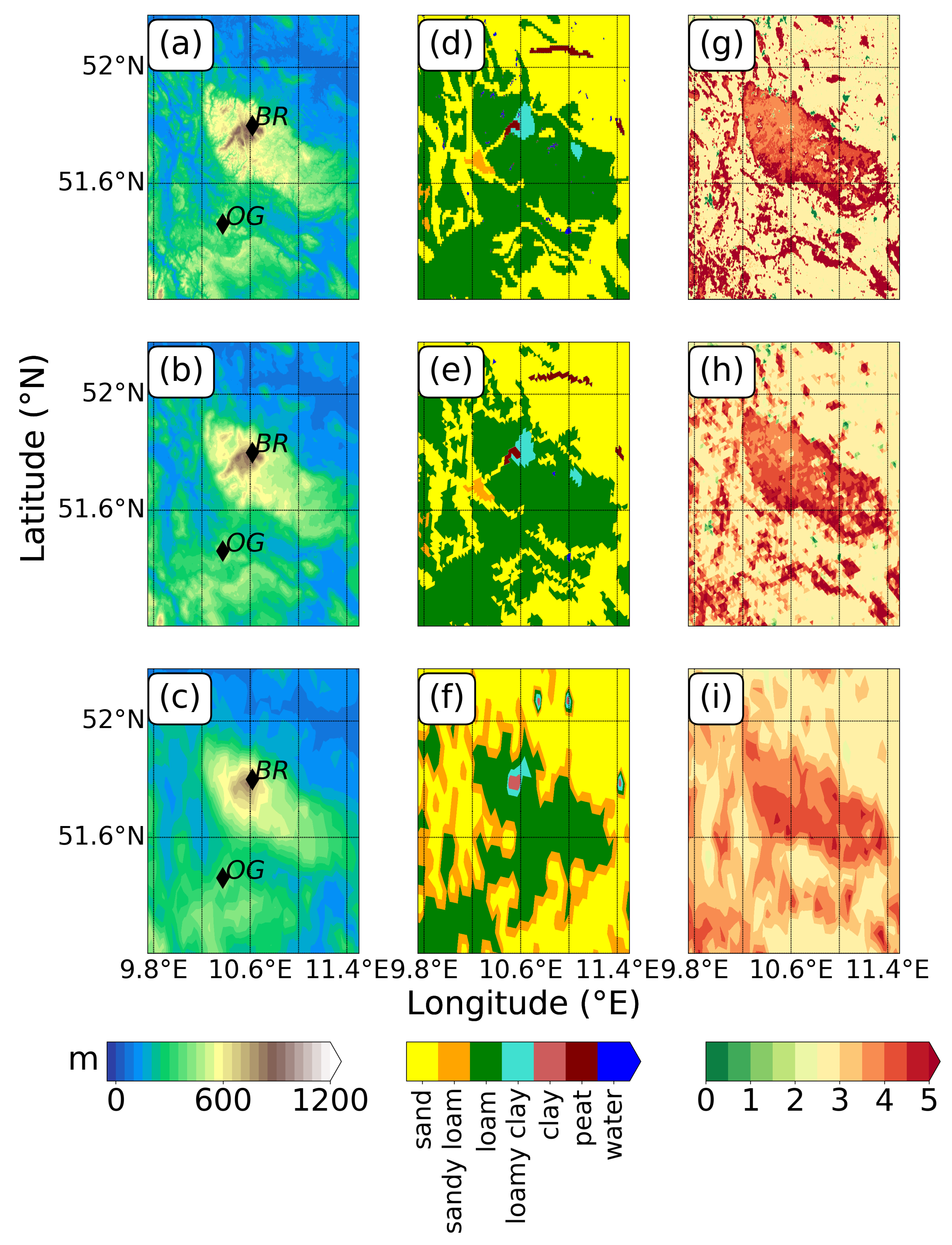
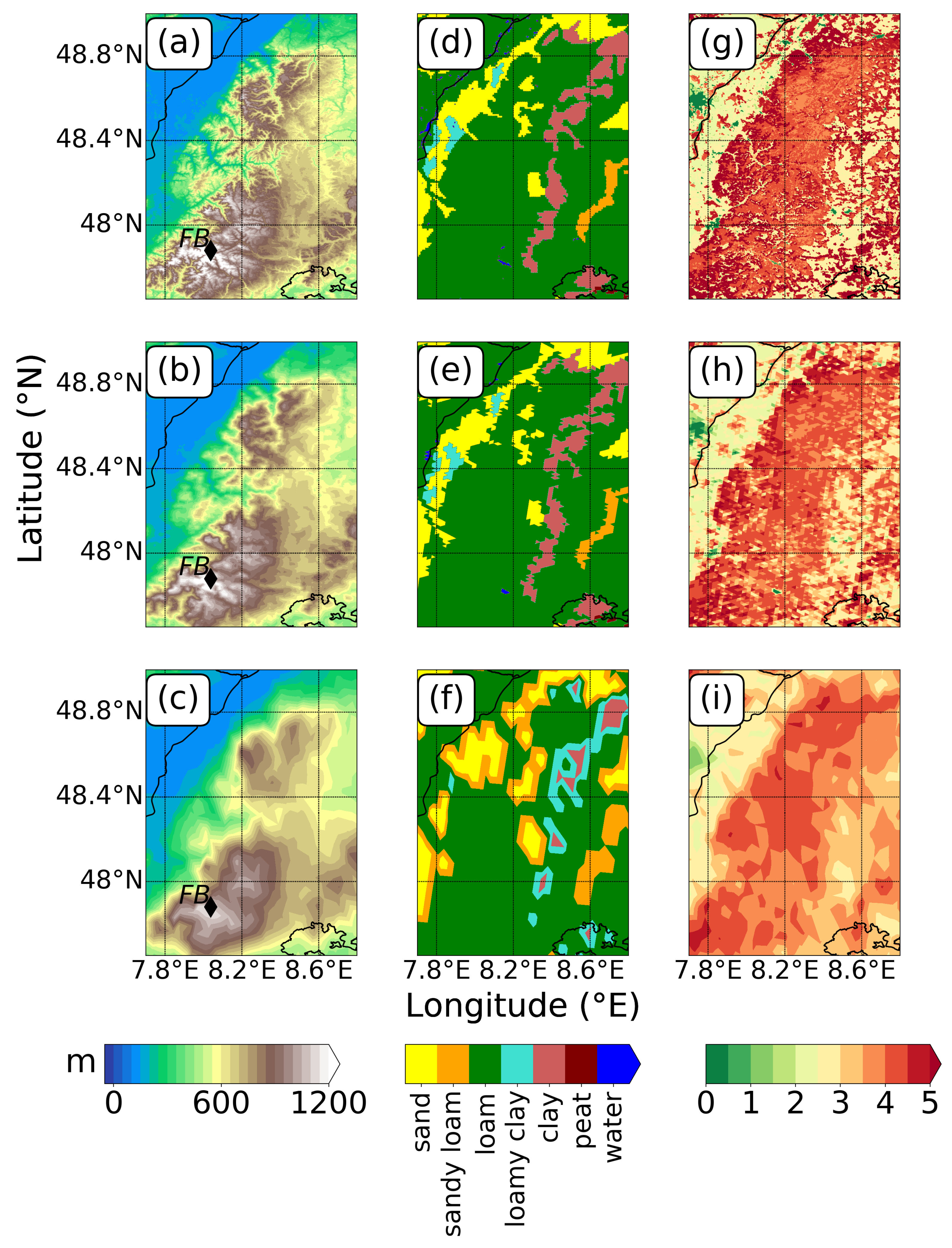
2.1. Investigation Areas and Selected Cases

In order to investigate the questions raised above, we performed simulations for two areas in Germany characterised by different degrees of land-surface heterogeneity, i.e., the relatively isolated and moderately high Harz mountains (HM) and the complex and higher Black Forest mountains (CT) (Figure 1a and Figure 2a). These regions are also characterised by a considerable degree of heterogeneity concerning soil type (Figure 1d and Figure 2d) and vegetation (Figure 1g and Figure 2g). Additionally, the selected cases are characterised with weak large-scale synoptic forcing and considerable convective precipitation (Radar Online Adjustment (RADOLAN)-RW [32] Figure 3g,h), i.e., horizontal wind speed at 850 hPa being <10 m s${}^{-1}$ (according to the ECMWF Re-Analysis (ERA)-Interim data set [33,34]) and lightning strikes >500 per 25 km${}^2$ (according to lightning data from Siemens lightning information service (BLIDS), which is part of the European Cooperation for Lightning Detection (EUCLID) [35]).

2.2. Model Setup and Simulation Strategy

The ICON model (version 2.3.0-nwp2), which has been developed at Deutscher Wetterdienst (DWD) and Max Planck Institute for Meteorology (MPI-M) [20,30,31], was used for this study. In ICON, the multi-layered soil-vegetation-atmosphere-transfer component (TERRA_ML) [36,37] acts as lower-boundary condition for the atmospheric part of ICON.

The ICON simulations were performed in the Large Eddy Model (LEM) mode. We used a one-way nesting setup, starting from the parent domain of grid spacing of 5000 m going to 2500 m using NumericalWeather Prediction (NWP) model physics (denoted as ${\Delta }_{5000}$ and ${\Delta }_{2500}$) and from 1250 m going down to 156 m using Large Eddy Simulation (LES) model physics (denoted as ${\Delta }_{1250}$, ${\Delta }_{625}$, ${\Delta }_{312}$ and ${\Delta }_{156}$). The sizes of the innermost domain are about 100 km × 150 km for HM and 150 km × 100 km for CT (Figure 1 and Figure 2). The NWP and LES model physics correspond to 1-D [38] and 3-D turbulence [39] parameterisation scheme, respectively. In the ‘grey zone’ or ‘terra incognita’ [24], only limited studies exist, which address at which model grid spacing an appropriate transition from a 1-D to 3-D turbulence parameterisation scheme should be applied [40,41]. As 156 to 1250 m grid spacings belong to the grey zone, we used the 3-D turbulence scheme based on the extended Smagorinsky model [39]. The setup uses 90 vertical levels with the model top level at 20 km and the lowermost minimum layer thickness at 10 m. The operational ICON analysis product ICON-Europe (ICON-EU) (grid spacing of 6.5 km and 60 vertical layers, source: [42]) was used for initial and boundary conditions of the ICON simulations. The boundary of the parent domain (${\Delta }_{5000}$) was relaxed towards three hourly ICON-EU assimilation forecast products. The selected cases described in Section 2.1 were simulated for 24 h with an initialisation at 00 UTC and output interval of 10 min. The analysis period excludes the possible spin-up time. For more details of the model configuration and physics set up, see [43].

To investigate the dependence of convective precipitation on land-surface resolution, we compare sensitivity runs with control runs. ${\Delta }_{156}$ is the control run. For the control run, the land-surface resolution is the same as the underlying model grid spacing. In the sensitivity runs, the model grid spacings remain at 156 m, while the resolutions of land-surface properties (L) and orography-related parameters (O) were coarsened to 1250 and 5000 m, respectively. Land-surface properties (L) include soil type, Transpiration Area Index (TAI), plant cover, Normalized Difference Vegetation Index (NDVI) and other land-surface parameters except orography. As a step of creating the external parameters, the software tool EXTPAR (External Parameter for Numerical Weather Prediction and Climate Application) is applied [44]. It takes the raw data and interpolates it on the target grid of ICON. The resolutions of source-raw data sets of some relevant external parameters are: 1${}^{″}$ (30 m) for orography, 10${}^{″}$ (300 m) for land cover parameters such as vegetation, plant cover, TAI etc. and 30${}^{″}$ (900 m) for soil type. There is no orographic smoothing filter from EXTPAR but the orography undergoes a smoothing during the model simulation, where a maximum height difference between adjacent grid points of 200 m is allowed for the different runs at 156 m model grid spacing.

In the sensitivity runs, the coarsening of orography related fields is performed by using the Barycentric interpolation method of DWD-ICON-tools [45]. Other static parameters of land surface properties (soil type, vegetation, plant cover etc.) are interpolated using area-weighted average method. The initial soil moisture in the sensitivity runs is the same as in the reference runs because the soil moisture is taken from the ICON-EU which is already at a coarser resolution (6.8 km) than the sensitivity runs (1 and 5 km). The Soil Moisture Index (SMI) in the sensitivity runs is calculated based on the soil moisture from ICON-EU and the targeted soil types at 1 and 5 km. ICON uses this SMI at the initialisation step. This results in a group of sensitivity runs that is based on (i) where orography and land-surface properties were coarsened altogether (denoted as $L{O}_{1250}$ and $L{O}_{5000}$), (ii) coarsened land-surface properties (denoted as $L_{1250}$ and $L_{5000}$) and (iii) coarsened orography (denoted as $O_{1250}$ and $O_{5000}$). The corresponding distributions of orography and land-surface properties (soil type, and TAI) are shown in Figure 1 for the Harz mountains and Figure 2 for the Black Forest mountains.

The Harz mountains is a north-west to south-east oriented mountain range in Northern Germany, about 120 km in length and 40 km in width (Figure 1a). Its highest elevation, the Brocken (BR, 1141 m asl) is situated in the northwestern part of the mountain range. At $O_{5000}$, the smaller valleys, visible at ${\Delta }_{156}$ and $O_{1250}$, are no longer resolved (Figure 1a–c) and the highest peaks of the mountain range are lowered by about 300 m (Figure 1c). The dominating soil type in the Harz mountains and Ohmgebirge is loam (Figure 1d). However, in the area around the Brocken, it is loamy clay and peat and only a stripe of sandy soil expands along a small valley to the southwest. Sandy soil also dominates the soil type north of the Harz mountains while loam mainly exists in the south. Coarsening of the land-surface resolution to 5000 m replaces the soil type of loam by soil type of sandy loam in the transition zone from the Harz mountain to the flat land (Figure 1f). At the Brocken, in $L_{5000}$ the soil type peat disappeared but a spot with clay and loamy clay remained in that area (Figure 1f). High TAI values (4–5) can be found over the forested Harz mountains and Ohmgebirge (highest along the slopes), while TAI is considerably lower in the agriculturally used flat surroundings (mainly 2–3) (Figure 1g). Villages and small towns, indicated by small TAI values at ${\Delta }_{156}$ and $L_{1250}$, are not longer resolved at $L_{5000}$ (Figure 1g–i).

The Black Forest mountains, located in the southwest of Germany, consist of two main mountain ranges, the northern and southern Black Forest. The Hornisgrinde (1164 m asl) in the northern and the Feldberg (FB, 1493 m above sea level (asl) in the southern Black Forest being their highest peaks (Figure 2a). While several valleys are visible at ${\Delta }_{156}$ and $O_{1250}$, the smaller ones are not resolved at $O_{5000}$ anymore (Figure 2a–c) and the top of the southern Black Forest is only 1160 m asl at $O_{5000}$. The Black Forest mountains are mainly characterised by soil type loam while sand is dominating in the Rhine valley west of the mountains (Figure 2d). Soil type clay is present in an elongated stripe east of the of the mountain range (Neckar valley). Note that at $L_{5000}$ this soil type along the valley is replaced by loamy clay but the stripe is still distinguishable from its surroundings (Figure 2f). Finally, the mountain range is characterised by higher TAI values (4–5), while the valley of the Black Forest and the areas west and east of the mountainous are indicated by TAI values ranging from 2–3 (Figure 2g,h). Villages and towns have TAI values < 1. In $L_{5000}$, the small valleys and villages are no longer resolved (Figure 2i) and only the Rhine valley, Black Forest mountain range and Neckar valley are mainly distinguishable.

2.3. Analysis Tools

Different analysis tools were used to understand the different phases of moist convection, i.e., from triggering of convection (applying multiple regression coefficients for surface-sensible heat flux (H) and surface-latent heat flux (E), convection indices, and backward trajectories) via evolution of clouds (calculating onset time of clouds and heat budget, cloud size distribution) to precipitation (calculating onset time and spatial patterns of precipitation). The tools are described in detail in the following.

Triggering of convection is normally related to the spatial distribution of turbulent surface fluxes. To identify the possible factors determining these fluxes, the areal mean Standardized Multiple Regression Coefficient (SMRC) [46] is calculated for surface-sensible heat flux (H) and surface-latent heat flux (E). The SMRC estimates how much increase in the explanatory variable affects its relative importance or position within the group for determination of the outcome variable ($H,E$). For example, the formulation for H is:

$$\begin{array}{c}\hfill {\mathrm{SMRC}}_H=b_k\ast \frac{{\sigma }_k}{{\sigma }_H},\end{array}$$

(1)

where k represents the explanatory variables (SMI, TAI, orography, net radiation, and horizontal wind speed at 10 m). $b_k$ is the coefficient estimate of H, and ${\sigma }_k$ and ${\sigma }_H$ are the standard deviations of the explanatory variables and the outcome variable (H), respectively. These variables are selected because they are assumed to be the most relevant parameters determining the partitioning of energy exchange at the Earth’s surface into the surface-sensible and latent heat flux, respectively. A high value of SMRC for an explanatory variable shows its more significant contribution to the determination of the outcome variable and vice versa.

Furthermore, the trajectories were calculated in order to trace back the source of convective systems. The trajectory tool LAGrangian ANalysis TOol (LAGRANTO) is applied [47]. LAGRANTO was designed essentially to calculate forward and backward trajectories of air parcels to identify the flow structures of air masses. To identify the source regions of air parcels of convective clouds, the backward trajectories starting from the cloud base or inside the cloud itself are calculated with LAGRANTO. The version LAGRANTO-ICON works on horizontal regular latitude-longitude. Therefore, the required trajectory fields are interpolated from ICON to a regular latitude-longitude grid. LAGRANTO uses 3-D wind fields namely (zonal wind u (in m s${}^{-1}$), meridional wind v (in m s${}^{-1}$) and vertical wind $\omega$ (in Pa s${}^{-1}$). Additionally, it needs surface pressure for the configuration of a level type, which further calculates the full 3-D pressure on the model fields and identifies the trajectory points intersecting the underlying orography. To study the local triggering, the vertical coordinate in meters is intended. Therefore, LAGRANTO needs the information of orography and the 3-D geopotential height for all grid points. The version adapted for ICON works also with a very high temporal resolution (up to 1 min) of model fields (in this study 10 min). For details of the different functionalities and their usage in LAGRANTO, see [48].

Another tool used in this analysis is the heat budget equation, which specifies the different contributions (divergence of the sensible heat flux, microphysics, vertical and horizontal advection, divergence of net radiation) to the net tendency of heat (${\theta }_v$), e.g., [16,49,50]. It has been implemented in ICON in online mode [43]. Here, we only discuss the contribution of microphysical processes to the tendency of heat, i.e., on the net body source terms associated with the phase changes ($MIC{R}_{{\theta }_v}$). For details of different budget terms, see [43].

Finally, to analyse the evolution of the clouds, the cloud-size distribution was calculated using the Python wrapper for OpenCV [51]. The cloud-size distributions were determined based on the equivalent diameter, which is the diameter of a circle with a surface area equal to the respective contour area of the cloud. Using the same wrapper, the Convective Organisation Potential (COP) [52] was calculated to quantify the degree of aggregation of clouds. For more information, we refer to [43].

3. Results

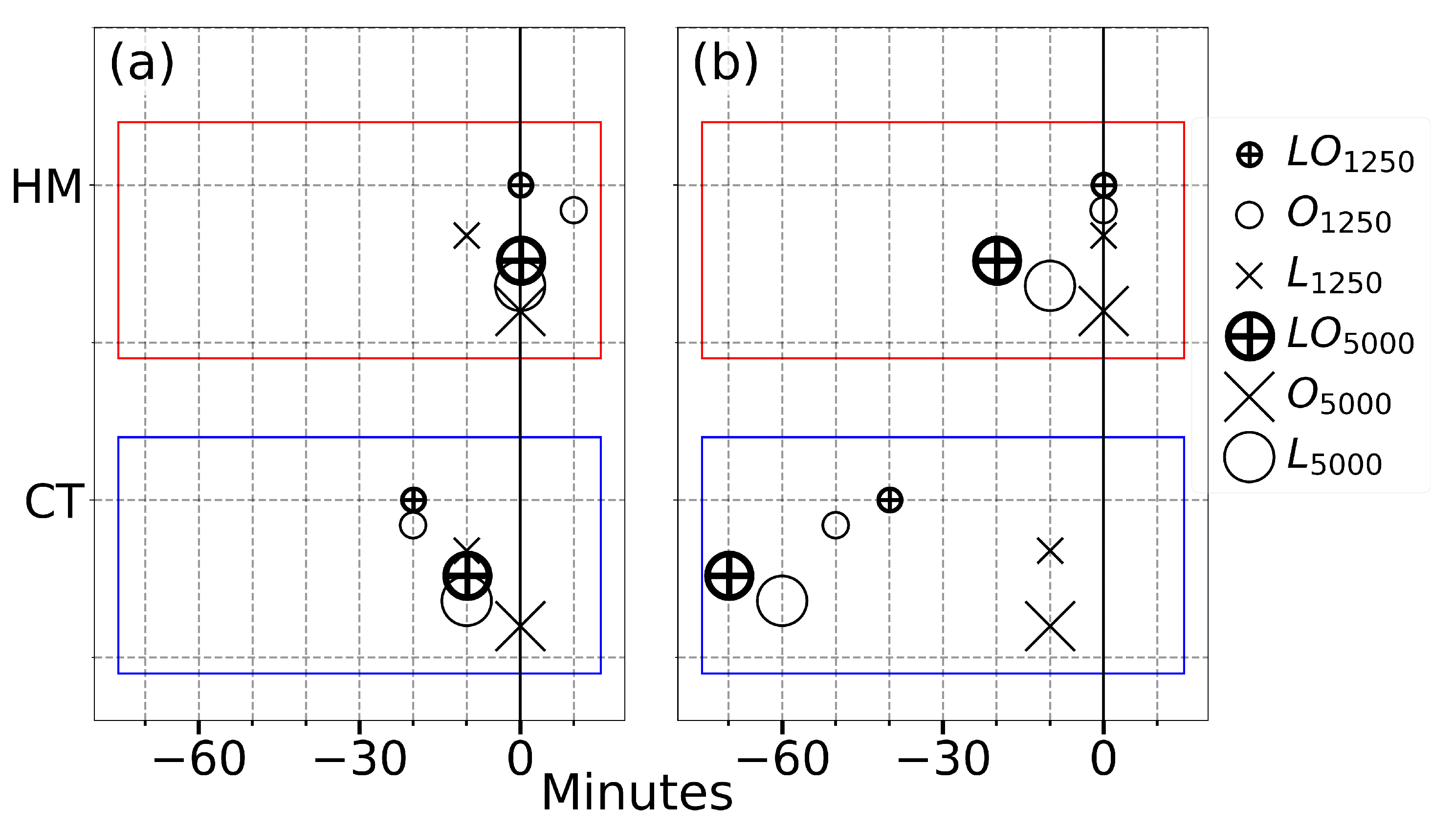
3.1. Areal Means in Dependence of Land-Surface Resolution

Table 1. The areal mean daily precipitation amount in control and sensitivity runs for the Harz mountain (HM) and Black Forest (CT).

Cases	${\mathbf{\Delta }}_{156}$	${\mathit{LO}}_{1250}$	${\mathit{L}}_{1250}$	${\mathit{O}}_{1250}$	${\mathit{LO}}_{5000}$	${\mathit{L}}_{5000}$	${\mathit{O}}_{5000}$
HM (9 June 2018)	0.91	0.92	0.99	0.95	1.06	0.94	1.14
CT (29 May 2017)	2.03	1.93	1.83	1.89	1.68	1.72	1.81

summarises the areal mean daily precipitation amount of the control and sensitivity runs at 156 m model grid spacing for HM and CT. We focus on two cases, in which the resolution of land-surface parameters leads to distinct differences in convective precipitation i.e., 9 June 2018 over HM and 29 May 2017 over CT. Coarsening the land-surface parameters led to relative differences between $L_{1250}$, $O_{1250}$ and $L{O}_{1250}$ and the control run of ≤10% and between $L_{5000}$, $O_{5000}$ and $L{O}_{5000}$ and the control run of ≤25%. There is no consistent impact of land-surface properties or orography on areal mean daily precipitation amount. On average, the relative difference increases with coarser resolution, i.e., is 6% for 1250 m and 15% for 5000 m. Nevertheless, temporal and spatial differences within the model domain between the control and sensitivity runs exist (Figure 3).

Over the Harz mountains, two distinct precipitation events occurred on 9 June 2018 which are shown in Figure 3a,c,e. In all three simulations (${\Delta }_{156}$, $L{O}_{1250}$, $L{O}_{5000}$), the north-western part of the Harz mountains, i.e., the Brocken and its surroundings (Figure 1a), were affected by the first major precipitation event. The accumulated precipitation in $L{O}_{5000}$ is higher than ${\Delta }_{156}$ (Figure 3a,e). The possible reasons for these differences in precipitation are given in Section 3.2.1. The temporal evolution of clouds and precipitation provides additional information. In ${\Delta }_{156m}$, the first convective clouds are simulated around 0920 Coordinated Universal Time (UTC) over the Harz mountain ridge (not shown). Concerning the sensitivity simulations based on coarsening of orography and land-surface properties, the onset of clouds does not differ that much from that in ${\Delta }_{156}$ (in the range of ±15 min, Figure 4a). Precipitation set in shortly after 1100 UTC (not shown), again the differences in onset times are small for all simulations (differences <30 min, Figure 4b). A second precipitation event, less strong and less spatially homogeneous compared to the first one, occurred along a southwest oriented stripe in southwest of the Brocken (Figure 3a,c,e). The Hovmöller plot shows that this precipitation event occurred much later (e.g., in ${\Delta }_{156}$ after 1240 UTC, Figure 5a). Reasons for these two precipitation events are given in Section 3.2.1 and Section 3.2.3.

Concerning the Black Forest mountains, the differences of the areal mean daily precipitation between ${\Delta }_{156}$, $L{O}_{1250}$ and $L{O}_{5000}$ are mainly caused especially by differences in the southern part of the mountains (Figure 3b,d,f). The centre with the most intense precipitation in $L{O}_{5000}$ lies about 20 km to the east of the one in ${\Delta }_{156}$. Furthermore, although cloud formation in $O_{5000}$ and $L{O}_{5000}$ is only slightly earlier (≤20 min) compared to ${\Delta }_{156}$, precipitation in both sensitivity runs on average set in earlier by about 1 h than in ${\Delta }_{156}$ (Figure 4a,b). Thus, in this case, by coarsening the orography, the onsets of cloud and precipitation vary more significantly than does coarsening of the land-surface properties. Therefore, we focus on the reasons causing the differences between ${\Delta }_{156}$ and $O_{5000}$ (Section 3.3).

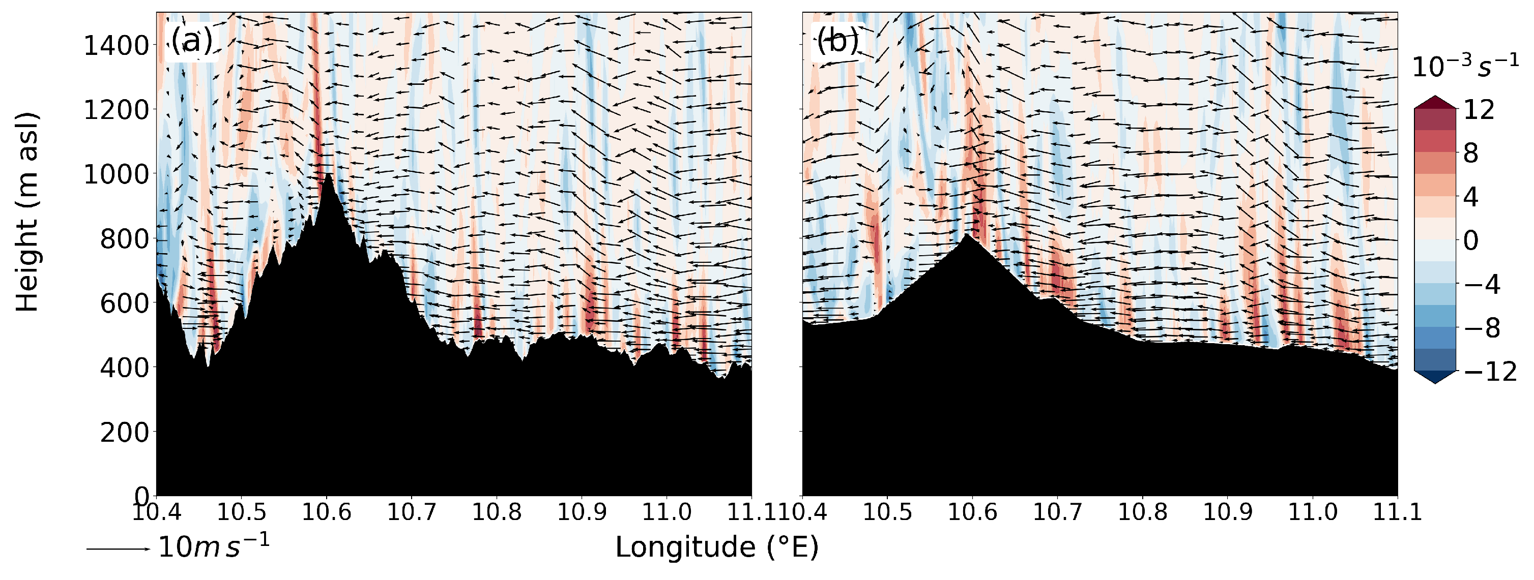
3.2. Processes Causing Convective Precipitation in Dependence on Land-Surface Resolution over an Isolated Mountain Range

In the following Section 3.2.1, we describe and analyse the main processes relevant for the first convective precipitation event over the Harz mountains on 9 June 2018 in the reference run (${\Delta }_{156}$) and in Section 3.2.2 we focus on the differences of the sensitivity run $O_{5000}$ to ${\Delta }_{156}$. Section 3.2.3 discusses the second precipitation event. $O_{5000}$ was selected because the results are similar to $L{O}_{5000}$ and the differences between ${\Delta }_{156}$ and $O_{5000}$ can be attributed to one cause (orography) only.

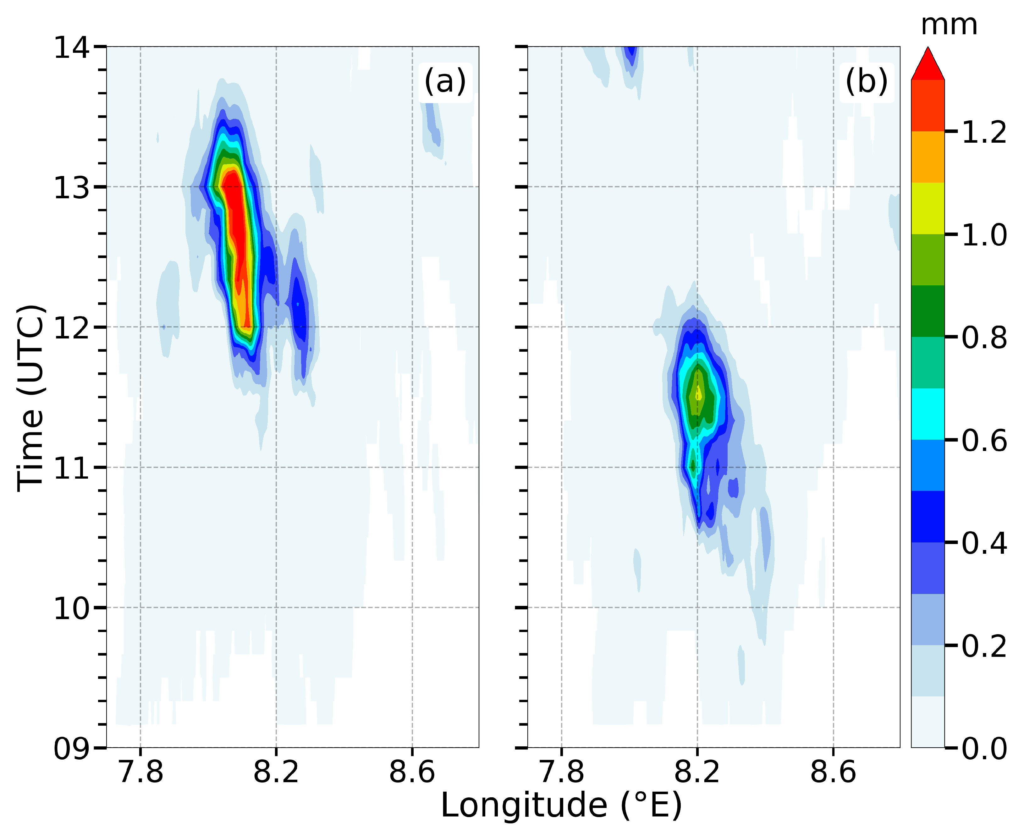
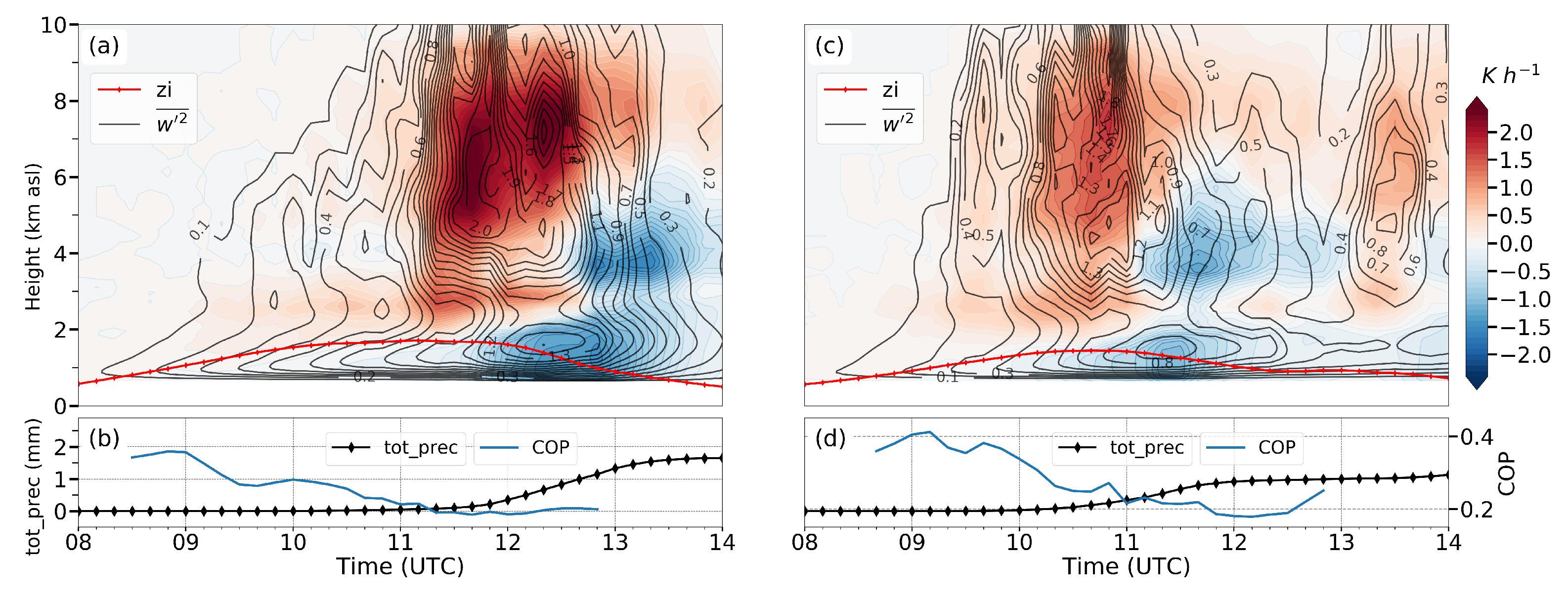
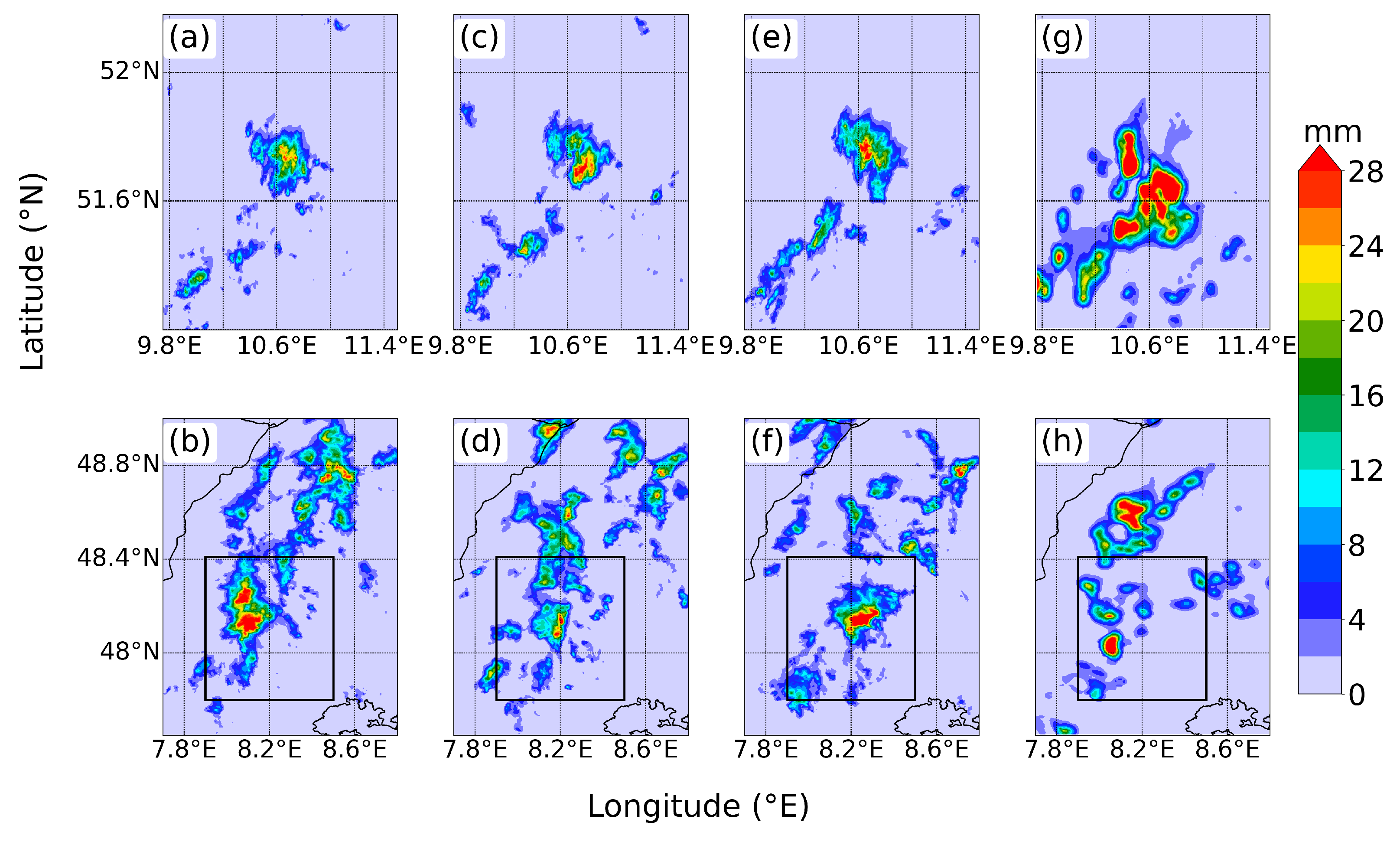
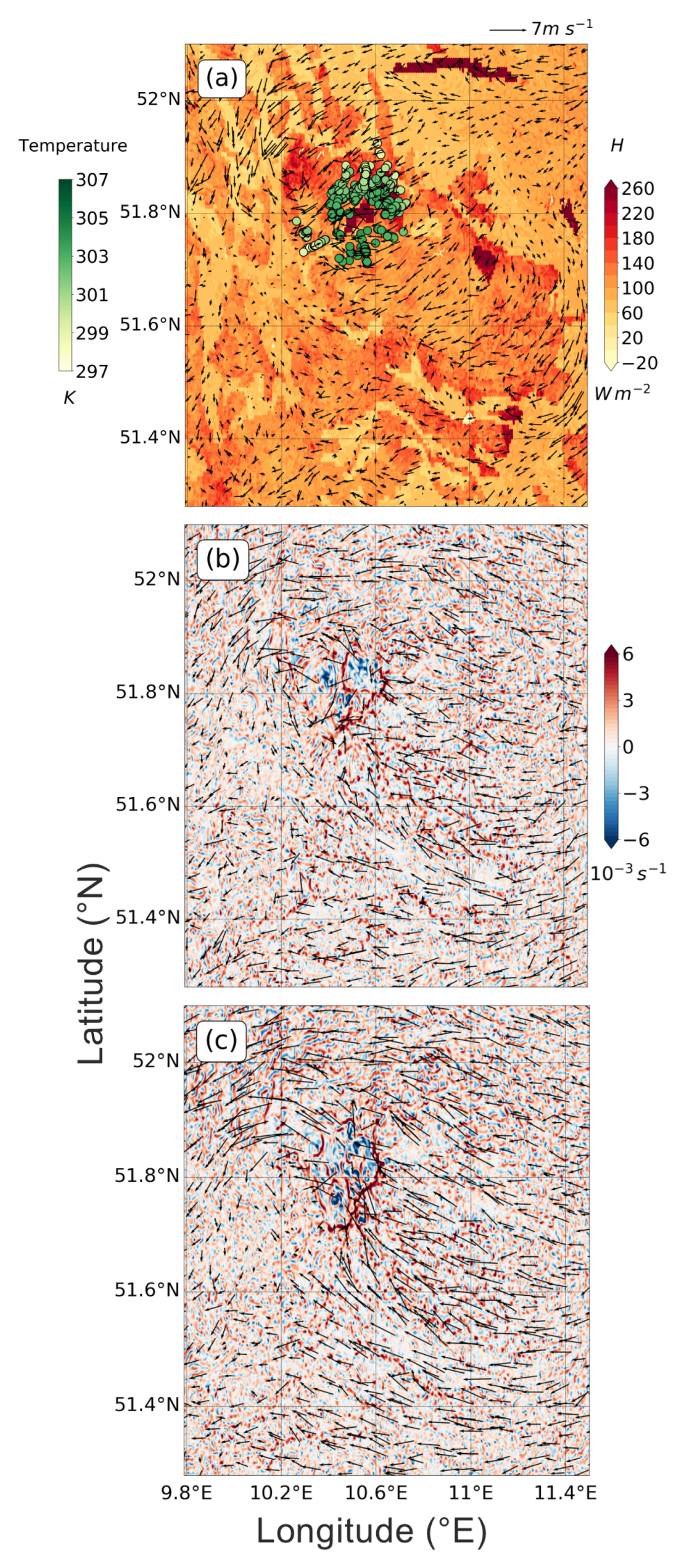
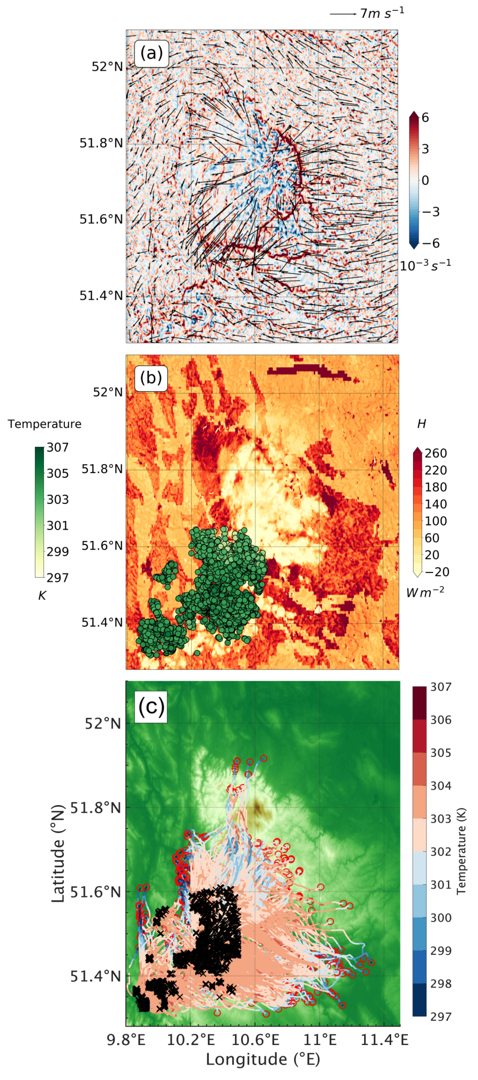
3.2.1. Reference Run—First Precipitation Event

With respect to land-surface heterogeneity, in ${\Delta }_{156}$ the first convection formed not only over the highest peaks of the Harz mountains but also over a region with the soil type of loamy clay and peat. The conditions, which led to the simulated precipitation are as follows: on 9 June 2018, an east-southeasterly large-scale wind prevailed in the Atmospheric Boundary Layer (ABL) (Figure 6a). Already at 0830 UTC, the spatial distribution of the surface-sensible heat flux shows higher values mainly over the higher elevations than over flat land. The surface-sensible heat flux ranges from a maximum value of up to 250 W m${}^{-2}$ over the spot with peat to about 150 W m${}^{-2}$ in the west of the Brocken. Surface-sensible heat flux values of about 100 to 120 W m${}^{-2}$ also prevailed in most of the remaining parts of the model domain (Figure 6a).

The $SMR{C}_H$ index indicates that H is well correlated with orography (≃+0.40) and SMI (≃−0.38), which is also reciprocated with a considerable correlation of E with orography (≃−0.42), SMI (≃+0.40), and TAI (≃+0.38). This means that the orography together with the soil type results in the simulated surface-sensible heat flux pattern with its maximum over the mountain ridge. Hence, these conditions favoured the strongest wind convergence over the northwestern part of this region. The near-surface wind field shows that up-slope winds on the slopes of the Harz mountains had developed already at 0830 UTC as well as up-valley winds in some of the valleys which extend from the foreland to the inner centre of the Harz mountains, such as the one in the southwest (Figure 6a). Within the next hours, these thermally-induced winds intensified resulting in the cloud formation over the Brocken. The horizontal wind convergence at 1100 UTC (Figure 6b) already indicates the onset of precipitation over that area.

The trajectories (not shown) starting at cloud base (≈1700 m asl) at 1100 UTC and then integrated backwards until 0700 UTC confirmed that the air parcels originate from near-surface positions of the surrounding flat forelands of the Harz mountains in the north and south. As transported upwards along the slopes of the Harz mountains by upslope winds, they reached the top of the Harz mountains at 0830 UTC (Figure 6a). At that time, all trajectories are concentrated within an area with a diameter of about 15 km over the Brocken. The convective precipitation that started at about 1110 UTC peaked between 1200 and 1300 UTC and stopped shortly afterwards over the Harz mountains (Figure 5a).

3.2.2. Differences of the Sensitivity Run to the Reference Run

The comparison of the precipitation patterns of ${\Delta }_{156}$ and $O_{5000}$ shows some more intense precipitation in $O_{5000}$ over the Brocken region (Figure 3a,e).

These differences can be mainly attributed to the modified boundary-layer wind field caused by the smoothing of the Harz mountains in $O_{5000}$ (Figure 1a,c and Figure 7). In $O_{5000}$, the southeasterly wind in the Convective Boundary Layer (CBL) was mainly able to flow over the Harz mountains instead of being forced to flow around them (Figure 6c and Figure 7b). This can be explained by the Froude number $Fr=U/\left(N{h}_0\right)$ [53], where U is the horizontal wind speed, $h_0$ the height of the obstacle and the Brunt–Vaisala frequency $N=\sqrt{\frac{g}{\overline{{\theta }_v}}{\theta }_{v}z}$. In $O_{5000}$, the Froude number for the boundary layer on the windward side of the Harz mountains at 1000 UTC is $Fr\approx$ 0.82 while in ${\Delta }_{156}$ is $Fr\approx$ 0.43. That means in $O_{5000}$, the flow above about 90 m agl approaching the Harz mountains had enough kinetic energy to flow over the mountain range, while in ${\Delta }_{156}$ only the flow higher than ≈ 450 m agl was able to do so. Additionally, in $O_{5000}$ the slope winds were deeper and stronger than in ${\Delta }_{156}$ (e.g., compare the slope wind systems west of the Brocken, Figure 7a,b). So, obviously both flows, i.e., the dynamically forced and thermally induced flow, were responsible for the stronger and wider wind convergence lines in $O_{5000}$ compared to ${\Delta }_{156}$ (Figure 6 and Figure 7). This finally caused the stronger convective precipitations over the Brocken region in $O_{5000}$ and $L{O}_{5000}$ compared to the one in ${\Delta }_{156}$ (Figure 3a,c,e and Figure 5a,b).

3.2.3. Reference Run—Second Precipitation Event

The second precipitation event was in continuation with the above-discussed Harz mountains case (Section 3.2.1). The temporal evolution of precipitation along a southwest oriented stripe, the Ohmgebirge (OG, indicated in Figure 1), southwest of the Brocken after 1300 UTC is similar in the ${\Delta }_{156}$ and $O_{5000}$ (Figure 5). As the underlying processes are comparable, we restrict ourselves to the analysis of the ${\Delta }_{156}$ results.

The area around the Ohmgebirge hills comprises of moderately elevated areas with some embedded valleys (Figure 1a). The first clouds established at about 1200 UTC (not shown). Maximum precipitation over this area amounted to ≈ 20 mm (Figure 3a). At 1230 UTC, the near-surface wind field mainly consists of three distinct branches causing wind converging in the southwest of the Harz mountains (Figure 8a). The first branch is the flow coming from southeast, which is the large-scale east-southeasterly wind deflected by the Harz mountains due to a low $Fr$ of ≈ 0.43 at 1000 UTC. The deep convective cell over the Brocken, discussed in the previous subsection, also supports a deflection of the approaching east-southeasterly wind. The second branch consists of the valley winds that blow from the west towards the Ohmgebirge. These valley winds are further assisted by the wind flowing around the Harz mountains in the north and turning into a northwesterly wind at the western tip of the Harz mountains. Finally, the third branch contributing effectively to wind convergence is the cold-pool outflow from the deep convective cell that previously formed over the Brocken. The gust front associated with the cold pool enhanced the wind convergence in the Ohmgebirge and ultimately triggered cloud formations. The role of the three flows, contributing to the wind convergence, becomes evident from the backward trajectories (Figure 8c). The trajectories were started from cloud bases at 1250 UTC and integrated backwards until 0900 UTC. The projections of the positions of the air parcels to the surface at 1230 UTC are shown in Figure 8b. We used air temperature of the air parcels along the trajectories to mark the outflow from the cold pool. The trajectory lines clearly visualise the contributions of the three aforementioned branches. This example quite well demonstrates the superpositioning effect of orography and land-surface properties as to where triggering occurs and the combined effect of dynamically- and thermally-induced wind convergence regarding secondary triggering of convection.

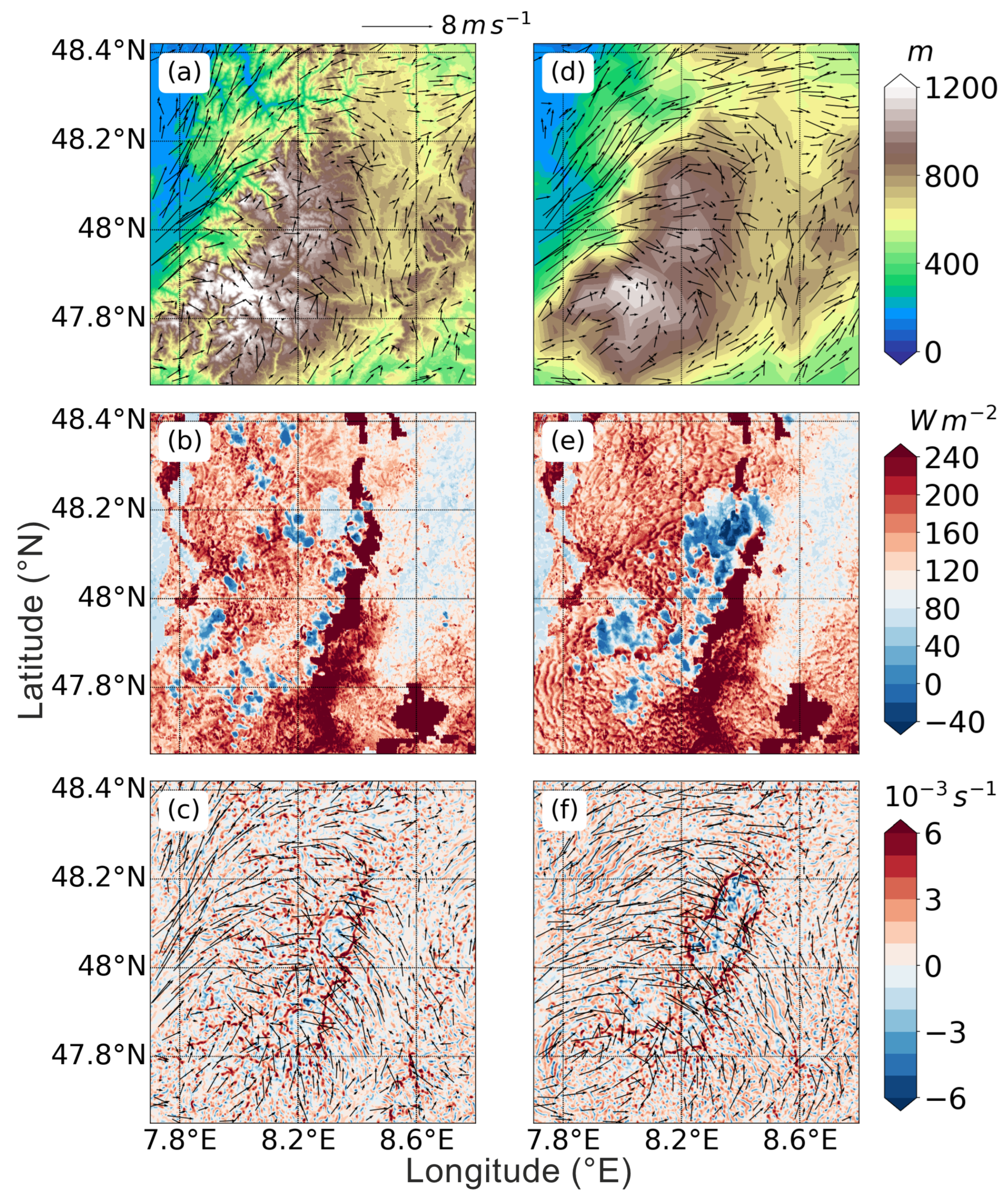
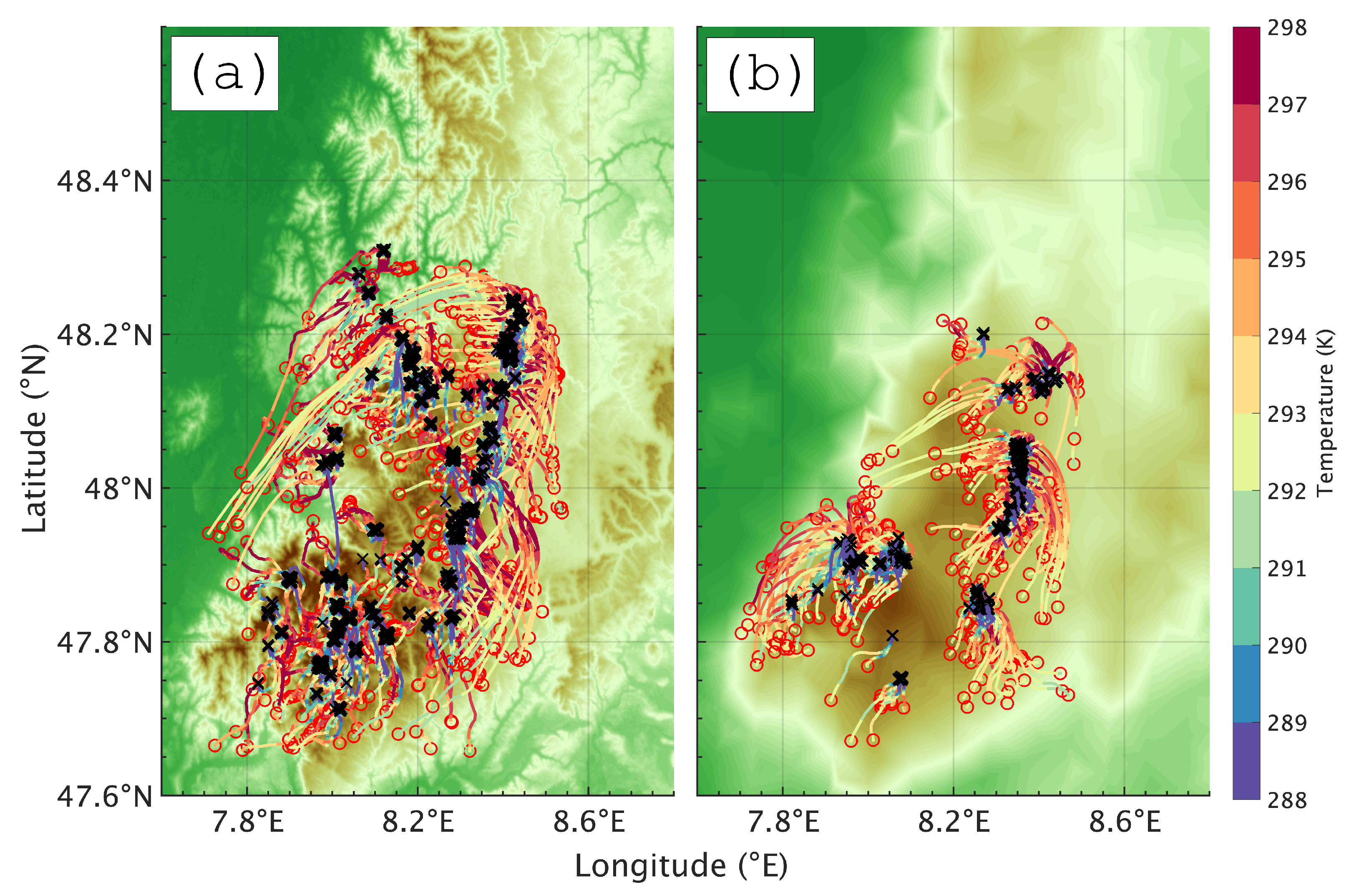
3.3. Processes Causing Convective Precipitation in Dependence on Land-Surface Resolution over Complex Terrain

A closer look at the spatio-temporal behaviour of precipitation in the southern Black Forest mountains (rectangular frame in Figure 3b,d,f) allows the Hovmöller diagram, laterally averaged from 47.650 to 48.417${}^{\circ }$ N (Figure 9). In ${\Delta }_{156}$, the intensive precipitation occurred around 8.1${}^{\circ }$ E at approximately 1140 UTC and in total lasted for about 2 h (Figure 9a). In $O_{5000}$, the precipitation started around 8.4${}^{\circ }$ E, i.e., east of the crests of the southern Black Forest mountains, already at about 1000 UTC (Figure 9b). Then, the maximum intensity of precipitation occurred further to the west reaching 8.2${}^{\circ }$ E at about 1130 UTC and precipitation stopped at approximately 1200 UTC. The precipitation intensity in ${\Delta }_{156}$ was considerably higher than that in $O_{5000}$. The processes relevant for the spatio-temporal evolution of convective precipitation in ${\Delta }_{156}$ are analysed in Section 3.3.1 and the reasons for the differences of $O_{5000}$ to ${\Delta }_{156}$ are presented in Section 3.3.2.

3.3.1. Reference Run

In ${\Delta }_{156}$ at 0900 UTC, southwesterly wind prevailed in the Rhine valley, slope winds were simulated on the southern, western and eastern slopes of the southern Black Forest mountains and, due to the highly resolved orography, valley winds developed in the small valleys of the southern Black Forest mountains (Figure 10a). Most of these mesoscale wind systems led to the formation of small clouds at 1000 UTC, identifiable by low or negative surface-sensible heat fluxes (Figure 10b). Part of these clouds are triggered over the Feldberg. This is also evident from the trajectories, starting at the cloud base (≃2800 m asl) at 1000 UTC and integrated backward until 0600 UTC (Figure 11a). Additionally, a more coherent north-south-oriented cloud band can be found along the lower part of the eastern slopes of the Black Forest mountains and Neckar valley (stretching approximately from 8.2${}^{\circ }$ E, 47.8${}^{\circ }$ N to 8.4${}^{\circ }$ E, 48.2${}^{\circ }$ N). This cloud band is associated with an anomaly of the surface-sensible heat flux, which already reached about 250 W m${}^{-2}$ over a north-south-oriented stripe, while the fluxes are much lower in the remaining part of the investigation area (Figure 10b). These higher surface-sensible heat fluxes occur over the clay soil (Figure 2d). Note that considerable low-level wind convergence and clouds developed over the transition zone from higher to lower surface-sensible heat fluxes (Figure 10b,c). Obviously, the surface-sensible heat flux anomaly is responsible for the offset of cloud formation from the Black Forest mountain ridge further to the east. This finding is supported by the backward trajectories which show that the cloud band is fed by parcels from the east but also from the west of the band with higher surface-sensible heat fluxes (Figure 10b,c and Figure 11a). However, according to the Hovmöller diagram (Figure 9a), these patchy clouds did not cause precipitation at that time and the reason will be explained in the following.

3.3.2. Differences of the Sensitivity Run to the Reference Run

In $O_{5000}$, as the small valleys are not resolved properly, its flow field at 0900 UTC is more homogeneous compared to ${\Delta }_{156}$ (Figure 10a,d). Slope winds are already present in most parts of the $O_{5000}$ model domain at this time. Additionally, the mean barrier height in the northern part of the southern Black Forest in $O_{5000}$ is smaller (650 m agl) compared to ${\Delta }_{156}$ (950 m agl), so that the Froude number in $O_{5000}$ is higher ($Fr=0.57$) than that in ${\Delta }_{156}$ ($Fr=0.37$). This explains the prevailing southwesterly wind between 48.0 and 48.2${}^{\circ }$ N in $O_{5000}$ resulting in a pronounced wind convergence where this southwesterly wind impinges on the southerly wind which exists east of the mountain ridge (Figure 10d,f).

The wind convergence in the boundary layer that is more intense in $O_{5000}$ than in ${\Delta }_{156}$ in the northern part of the southern Black Forest mountains during the morning hours (Figure 10c,f) caused more extended clouds (Figure 10b,e). The backward trajectories confirm that near-surface air from the Rhine valley partly fed these clouds (Figure 11b). Subsequently, the clouds evolved into deep convection and were responsible for the main precipitation event that set in already around 1000 UTC (Figure 9b). As the north-south-oriented stripe with clay soil is still mostly resolved in $O_{5000}$ (Figure 2f), the corresponding surface-sensible heat flux anomaly also creates a line of major low-level wind convergence east of the Black Forest mountain ridge (Figure 10f). The associated clouds are again fed by air parcels from both sides of the surface-sensible heat flux anomaly (Figure 10e and Figure 11b). The third area of main low-level wind convergence and related cloud formation can be found over the Feldberg (Figure 10e). Later on, when the slope winds dominate the wind field of the southern Black Forest, the clouds and precipitation concentrate along the mountain crests, as visible from the Hovmöller diagram, i.e., the precipitation shifts to around 8.2${}^{\circ }$ E (Figure 9b).

The reason for the delayed and westward shifted but more intense precipitation in ${\Delta }_{156}$ than in $O_{5000}$ (Figure 9) was examined based on the microphysical processes in combination with parameters such as the variance of the vertical wind speed, $\overline{w^{\prime 2}}$, and the COP (Figure 12). Note that this figure contains areal means for the region shown in Figure 10. Until 0930 UTC, the evolution in ${\Delta }_{156}$ and $O_{5000}$ is similar, i.e., turbulence developed in the growing CBL and some isolated clouds (COP ≈ 0.38) were formed.

In $O_{5000}$, deep convection already developed in the free troposphere between 0930 UTC and 1000 UTC, indicated by considerable variance of the vertical wind speed up to $\overline{w^{\prime 2}}$ = 0.5 m${}^2$s${}^{-2}$ and latent heat release of up to $MIC{R}_{{\theta }_v}$ = 0.5 K h${}^{-1}$ (Figure 12c). Figure 13b shows a cross section of $MIC{R}_{{\theta }_v}$ at 48.15${}^{\circ }$ N at 0930 UTC. The deep convective cell in the northern part of the southern Black Forest (Figure 10e) is dominated by latent heat release up to 10 km asl, including the cloud top. Negative $MIC{R}_{{\theta }_v}$ values are restricted to a small lateral entrainment zone. After about 1000 UTC, areal means of latent heat release and vertical wind variance increased considerably, COP decreased and precipitation set in (Figure 9b and Figure 12c,d). Convective precipitation occurred between 1000 to 1200 UTC in the northern part of the southern Black Forest mountains.

In contrast, in ${\Delta }_{156}$ after 0930 UTC the vertical wind variance and positive latent heat release in the free troposphere were still restricted to about approximately 3 to 5 km asl (Figure 12a). The net areal negative $MIC{R}_{{\theta }_v}$ values around 4 km asl indicate considerable cloud dissolution due to lateral de- and entrainment processes between the clouds and the dry environment. As reported by [43], this especially holds for conditions when on average, the clouds are small. An example of this microphysical effect is shown in Figure 13a. The diagram shows a vertical cross section at 48.15${}^{\circ }$ N at 0930 UTC, i.e., through the small clouds existing in ${\Delta }_{156}$ (Figure 10b). Entrainment processes active laterally and at the top of the clouds are simulated and prevent the clouds to grow through the dry layer around 4 km asl. The net areal negative $MIC{R}_{{\theta }_v}$ values in this layer indicate that the process of cloud dissolution, i.e., preventing clouds to grow deep, was active in ${\Delta }_{156}$ until about 1100 UTC (Figure 12a). $MIC{R}_{{\theta }_v}$ and $\overline{w^{\prime 2}}$ only increased considerably after approximately 1120 UTC. This is when the slope and valley winds in the southern Black Forest mountains were fully established, causing considerable wind convergence along the mountain ridge so that the clouds aggregated, indicated by a COP value of 0.4 (Figure 12b), and precipitation started (Figure 9a and Figure 12b). Hence, why, where and when moist convection was triggered and developed over complex terrain depended on the land-surface properties and orography while microphysical processes act further down the line to amplify differences between different lower boundary conditions.

4. Summary

In this study, we applied the ICON model in LES physics mode for control runs at a model grid spacing of 156 m (${\Delta }_{156}$). We also performed sensitivity runs at the same grid spacings with different land-surface resolutions (1250 m, 5000 m) both of orography (O) and/or land-surface properties (L). The focus is on understanding the relevant processes responsible for differences in convective precipitation (onset time and amount of precipitation), caused by the resolution of the different land-surface parameters. We focused on two days, when the modification of land-surface resolution resulted in considerable differences of convective precipitation.

In order to analyse the different model results, we used analysis tools such as the multi-regression analysis for determining the dependence of the surface heat fluxes on the environmental conditions (TAI, SMI, near-surface wind speed, radiation and orography), backward trajectories in order to identify the source areas of convection, heat budget of the atmosphere to understand the evolution of the clouds, and COP to estimate the degree of cloud aggregation.

The selected areas were characterised by different complexities in terms of orography and land-surface properties, that is an isolated mountain range (Harz mountains, HM) and complex terrain (Black Forest mountains, CT). The chosen days were characterised by weak synoptic forcing so that initiation of convection could be expected to be dominated by thermally-induced circulations and dynamically-driven flows. The main findings can be summarised as follows:

With regard to the impact of resolution of land-surface parameters on areal (≈15 × 10${}^3$ km${}^2$) mean daily precipitation, the relative difference between the control run and the sensitivity runs $L_{1250}$, $O_{1250}$ and $L{O}_{1250}$ it was ≤10% (6% on average) and the sensitivity runs $L_{5000}$,$O_{5000}$ and $L{O}_{5000}$ it was ≤25% (15% on average). The impact of land-surface properties or orography on areal mean daily precipitation is not consistent for the investigated cases. The onset time of areal mean clouds between sensitivity runs and control run differed by <20 min. However, in the Black Forest mountains the onset time of areal mean precipitation of $O_{5000}$ and $L{O}_{5000}$ differed by 1 h, while in $L_{5000}$ it differed by only 10 min to the control run. The onset time differences of areal mean precipitation could be explained by different processes active in the model domains.

In the case of the Harz mountains, orography and land-surface properties superimposed in a way that the strongest wind convergence developed over the mountain peak Brocken. Therefore, over this area, the clouds were triggered, followed by deep convection and precipitation in the late morning hours. The convection initiation was independent from the resolution of land-surface properties as the governing soil-type anomalies were still resolved at $L_{5000}$. In the case of a flattened orography ($O_{5000}$) the prevailing east-southeasterly wind in the ABL was able to flow over the Harz mountain ridge due to high $Fr=0.82$, while the flow splits into two branches and blew north and south around the Harz mountain in ${\Delta }_{156}$ ($Fr=0.43$). Additionally, in the morning the slope winds were stronger and deeper in $O_{5000}$ than in ${\Delta }_{156}$. Thus, dynamically and thermally-induced winds superimposed in a favourable manner leading to a stronger wind convergence over the Brocken and by this $O_{5000}$ and $L{O}_{5000}$ resulted in heavier precipitation compared to ${\Delta }_{156}$. Another phenomenon, the secondary triggering of convection, was also active on that day. The two branches of dynamically driven flows around the Harz mountains, the one in the north and the one in the south, caused wind convergence in the southwestern part of the Harz mountains (Ohmgebirge). The cold-pool outflow of the previous deep convection over the Brocken then contributed and enhanced the wind convergence over the Ohmgebirge and triggered secondary convection in the early afternoon.

The more complex terrain case, i.e., the Black Forest mountains, revealed significant differences between ${\Delta }_{156}$ and $O_{5000}$ with respect to the onset time of clouds and precipitation along with differences in their spatial occurrence. In $O_{5000}$, clouds and precipitation were simulated about 1 h earlier and about 20 km further east than in ${\Delta }_{156}$. The spatial distribution of the land-surface properties and the smoothed orography could be used for explanation. Especially the north-south elongated stripe with soil-type clay in the Neckar valley east of the Black Forest mountains played a decisive role. The soil-type anomaly, which was the same in ${\Delta }_{156}$ and $O_{5000}$, led to higher surface-sensible heat fluxes compared to the surroundings which caused wind convergence and the first formation of clouds in the morning. In ${\Delta }_{156}$, as the large-scale flow was mainly forced around the Black Forest mountains ($Fr=0.37$), moist convection developed when the slope and valley winds along the mountain ridge reached their mature state around noontime and when cloud aggregation reduced lateral de- and entrainment between the clouds and its dry mid-tropospheric environment. In $O_{5000}$, as the whole Black Forest mountains are flattened ($Fr=0.57$), the large-scale southwesterly wind partly flew over instead of around the main mountain ridge and, by this, enhanced the thermally-induced wind convergence in the east of the Black Forest mountains. Therefore, clouds grew deep and precipitation started already around an hour earlier compared to ${\Delta }_{156}$. Hence, concerning convection initiation both land-surface parameters, soil-type and orography, were active in competition and determined where and when the first clouds formed. Concerning more intense precipitation in ${\Delta }_{156}$ than in $O_{5000}$, cloud aggregation, which was favoured over the Black Forest mountains crests, was the most important factor.

So, it turned out that mesoscale-sized land-surface properties could both act in competition or optimal addition to orography with respect to convection initiation. The resolution of orography on thermally- and dynamically-induced flows had two consequences. In $O_{5000}$, the thermal wind systems were already more developed earlier in the morning than in ${\Delta }_{156}$. Additionally, $O_{5000}$ allowed a deeper layer of the impinging flow to cross the mountain than ${\Delta }_{156}$. Both factors favoured an earlier and stronger boundary-layer wind convergence and initiation of convective clouds in $O_{5000}$ than ${\Delta }_{156}$. Microphysical and cloud aggregation processes have proven to be important for further development from boundary-layer clouds into deep convection.

References

1. Weckwerth, T.M.; Parsons, D.B. A review of convection initiation and motivation for IHOP_2002. Mon. Weather Rev. 2006, 134, 5–22. [Google Scholar] [CrossRef]
2. Bennett, L.J.; Browning, K.A.; Blyth, A.M.; Parker, D.J.; Clark, P.A. A review of the initiation of precipitating convection in the United Kingdom. Q. J. R. Meteorol. Soc. 2006, 132, 1001–1020. [Google Scholar] [CrossRef]
3. Kirshbaum, D.J.; Adler, B.; Kalthoff, N.; Barthlott, C.; Serafin, S. Moist orographic convection: Physical mechanisms and links to surface-exchange processes. Atmosphere 2018, 9, 80. [Google Scholar] [CrossRef] [Green Version]
4. Schneider, L.; Barthlott, C.; Barrett, A.I.; Hoose, C. The precipitation response to variable terrain forcing over low mountain ranges in different weather regimes. Q. J. R. Meteorol. Soc. 2018, 144, 970–989. [Google Scholar] [CrossRef]
5. Heim, C.; Panosetti, D.; Schlemmer, L.; Leuenberger, D.; Schär, C. The influence of the resolution of orography on the simulation of orographic moist convection. Mon. Weather Rev. 2020, 148, 2391–2410. [Google Scholar] [CrossRef] [Green Version]
6. Schädler, G. Triggering of atmospheric circulations by moisture inhomogeneities of the earth’s surface. Bound.-Layer Meteorol. 1990, 51, 1–29. [Google Scholar] [CrossRef]
7. Segal, M.; Arritt, R. Nonclassical mesoscale circulations caused by surface sensible heat-flux gradients. Bull. Am. Meteorol. Soc. 1992, 73, 1593–1604. [Google Scholar] [CrossRef] [Green Version]
8. Taylor, C.M.; Parker, D.J.; Harris, P.P. An observational case study of mesoscale atmospheric circulations induced by soil moisture. Geophys. Res. Lett. 2007, 34, L15801. [Google Scholar] [CrossRef] [Green Version]
9. Kottmeier, C.; Kalthoff, N.; Barthlott, C.; Corsmeier, U.; Van Baelen, J.; Behrendt, A.; Behrendt, R.; Blyth, A.; Coulter, R.; Crewell, S.; et al. Mechanisms initiating deep convection over complex terrain during COPS. Meteorol. Z. 2008, 17, 931–948. [Google Scholar] [CrossRef] [Green Version]
10. Kalthoff, N.; Adler, B.; Barthlott, C.; Corsmeier, U.; Mobbs, S.; Crewell, S.; Träumner, K.; Kottmeier, C.; Wieser, A.; Smith, V.; et al. The impact of convergence zones on the initiation of deep convection: A case study from COPS. Atmos. Res. 2009, 93, 680–694. [Google Scholar] [CrossRef]
11. Klüpfel, V.; Kalthoff, N.; Gantner, L.; Taylor, C.M. Convergence zones and their impact on the initiation of a mesoscale convective system in West Africa. Q. J. R. Meteorol. Soc. 2012, 138, 950–963. [Google Scholar] [CrossRef] [Green Version]
12. Schlemmer, L.; Hohenegger, C. The formation of wider and deeper clouds as a result of cold-pool dynamics. J. Atmos. Sci. 2014, 71, 2842–2858. [Google Scholar] [CrossRef] [Green Version]
13. Hirt, M.; Craig, G.C.; Schäfer, S.A.; Savre, J.; Heinze, R. Cold-pool-driven convective initiation: Using causal graph analysis to determine what convection-permitting models are missing. Q. J. R. Meteorol. Soc. 2020, 146, 2205–2227. [Google Scholar] [CrossRef]
14. Clark, D.B.; Taylor, C.M.; Thorpe, A.J. Feedback between the land surface and rainfall at convective length scales. J. Hydrometeorol. 2004, 5, 625–639. [Google Scholar] [CrossRef]
15. Barthlott, C.; Kalthoff, N. A numerical sensitivity study on the impact of soil moisture on convection-related parameters and convective precipitation over complex terrain. J. Atmos. Sci. 2011, 68, 2971–2987. [Google Scholar] [CrossRef]
16. Adler, B.; Kalthoff, N.; Gantner, L. Initiation of deep convection caused by land-surface inhomogeneities in West Africa: A modelled case study. Meteorol. Atmos. Phys. 2011, 112, 15–27. [Google Scholar] [CrossRef]
17. Hohenegger, C.; Schlemmer, L.; Silvers, L. Coupling of convection and circulation at various resolutions. Tellus A 2015, 67, 26678. [Google Scholar] [CrossRef] [Green Version]
18. Panosetti, D.; Böing, S.; Schlemmer, L.; Schmidli, J. Idealized large-eddy and convection-resolving simulations of moist convection over mountainous terrain. J. Atmos. Sci. 2016, 73, 4021–4041. [Google Scholar] [CrossRef]
19. Liu, S.; Shao, Y.; Kunoth, A.; Simmer, C. Impact of surface-heterogeneity on atmosphere and land-surface interactions. Environ. Model. Softw. 2017, 88, 35–47. [Google Scholar] [CrossRef]
20. Heinze, R.; Dipankar, A.; Henken, C.C.; Moseley, C.; Sourdeval, O.; Trömel, S.; Xie, X.; Adamidis, P.; Ament, F.; Baars, H.; et al. Large-eddy simulations over Germany using ICON: A comprehensive evaluation. Q. J. R. Meteorol. Soc. 2017, 143, 69–100. [Google Scholar] [CrossRef] [Green Version]
21. Stevens, B.; Acquistapace, C.; Hansen, A.; Heinze, R.; Klinger, C.; Klocke, D.; Rybka, H.; Schubotz, W.; Windmiller, J.; Adamidis, P.; et al. The added value of large-eddy and storm-resolving models for simulating clouds and precipitation. J. Meteorol. Soc. Jpn. 2020, 98, 395–435. [Google Scholar] [CrossRef] [Green Version]
22. Weisman, M.L.; Skamarock, W.C.; Klemp, J.B. The resolution dependence of explicitly modeled convective systems. Mon. Weather Rev. 1997, 125, 527–548. [Google Scholar] [CrossRef]
23. Honnert, R. Representation of the grey zone of turbulence in the atmospheric boundary layer. Adv. Sci. Res. 2016, 13, 63–67. [Google Scholar] [CrossRef]
24. Wyngaard, J.C. Toward numerical modeling in the “Terra Incognita”. J. Atmos. Sci. 2004, 61, 1816–1826. [Google Scholar] [CrossRef]
25. Honnert, R.; Efstathiou, G.A.; Beare, R.J.; Ito, J.; Lock, A.; Neggers, R.; Plant, R.S.; Shin, H.H.; Tomassini, L.; Zhou, B. The Atmospheric Boundary Layer and the “Gray Zone” of Turbulence: A critical review. J. Geophys. Res. 2020, 125, e2019JD030317. [Google Scholar] [CrossRef]
26. Zhou, B.; Simon, J.S.; Chow, F.K. The convective boundary layer in the terra incognita. J. Atmos. Sci. 2014, 71, 2545–2563. [Google Scholar] [CrossRef]
27. Chow, F.K.; Weigel, A.P.; Street, R.L.; Rotach, M.W.; Xue, M. High-resolution large-eddy simulations of flow in a steep Alpine valley. Part I: Methodology, verification, and sensitivity experiments. J. Appl. Meteorol. Climatol. 2006, 45, 63–86. [Google Scholar] [CrossRef] [Green Version]
28. Barthlott, C.; Hoose, C. Spatial and temporal variability of clouds and precipitation over Germany: Multiscale simulations across the “gray zone”. Atmos. Chem. Phys. 2015, 15, 12361–12384. [Google Scholar] [CrossRef] [Green Version]
29. Singh, S. Convective Precipitation Simulated with ICON over Heterogeneous Surfaces in Dependence on Model and Land-Surface Resolution; Karlsruhe Institute of Technology (KIT) Scientific Publishing: Karlsruhe, Germany, 2021; p. 200. [Google Scholar] [CrossRef]
30. Zängl, G.; Reinert, D.; Rípodas, P.; Baldauf, M. The ICON (ICOsahedral Non-hydrostatic) modelling framework of DWD and MPI-M: Description of the non-hydrostatic dynamical core. Q. J. R. Meteorol. Soc. 2015, 141, 563–579. [Google Scholar] [CrossRef]
31. Dipankar, A.; Stevens, B.; Heinze, R.; Moseley, C.; Zängl, G.; Giorgetta, M.; Brdar, S. Large eddy simulation using the general circulation model ICON. J. Adv. Model. Earth Syst. 2015, 7, 963–986. [Google Scholar] [CrossRef] [Green Version]
32. Bartels, H.; Weigl, E.; Reich, T.; Lang, P.; Wagner, A.; Kohler, O.; Gerlach, N. Projekt RADOLAN–Routineverfahren zur Online-Aneichung der Radarniederschlagsdaten mit Hilfe von automatischen Bodenniederschlagsstationen (Ombrometer). Dtsch. Wetterdienst, Hydrometeorol. 2004, 5. [Google Scholar]
33. Berrisford, P.; Dee, D.; Poli, P.; Brugge, R.; Fielding, K.; Fuentes, M.; Kallberg, P.; Kobayashi, S.; Uppala, S.; Simmons, A. The ERA-Interim archive, version 2.0. ERA Rep. Ser. 2011, 1, 23. Available online: https://www.ecmwf.int/node/8174 (accessed on 10 May 2022).
34. Dee, D.P.; Uppala, S.M.; Simmons, A.; Berrisford, P.; Poli, P.; Kobayashi, S.; Andrae, U.; Balmaseda, M.; Balsamo, G.; Bauer, d.P.; et al. The ERA-Interim reanalysis: Configuration and performance of the data assimilation system. Q. J. R. Meteorol. Soc. 2011, 137, 553–597. [Google Scholar] [CrossRef]
35. Schulz, W.; Diendorfer, G.; Pedeboy, S.; Poelman, D.R. The European lightning location system EUCLID–Part 1: Performance analysis and validation. Nat. Hazards Earth Syst. Sci. 2016, 16, 595–605. [Google Scholar] [CrossRef] [Green Version]
36. Schrodin, R.; Heise, E. The Multi-Layer Version of the DWD Soil Model TERRA_LM; COSMO Technical Report No. 2; Deutscher Wetterdienst (DWD): Offenbach, Germany, 2001. [Google Scholar] [CrossRef]
37. Heise, E.; Ritter, B.; Schrodin, R. Operational implementation of the multilayer soil model. Consort. Small-Scale Model. (COSMO) Tech. Rep. 2006, 9, 20. [Google Scholar]
38. Raschendorfer, M. The new turbulence parameterization of LM. Proc. Cosmo Newsl. 2001, 1, 89–97. Available online: http://www.cosmo-model.org/content/model/documentation/newsLetters/newsLetter01/newsLetter_01.pdf (accessed on 10 May 2022).
39. Lilly, D.K. On the numerical simulation of buoyant convection. Tellus 1962, 14, 148–172. [Google Scholar] [CrossRef]
40. Honnert, R.; Masson, V. What is the smallest physically acceptable scale for 1D turbulence schemes? Front. Earth Sci. 2014, 2, 27. [Google Scholar] [CrossRef] [Green Version]
41. Cuxart, J. When can a high-resolution simulation over complex terrain be called LES? Front. Earth Sci. 2015, 3, 87. [Google Scholar] [CrossRef] [Green Version]
42. DWD-PAMORE. PArallel MOdel Data REtrieve from Oracle Databases (PAMORE); Deutscher Wetterdienst (DWD): Offenbach, Germany, 2015. [Google Scholar]
43. Singh, S.; Kalthoff, N.; Gantner, L. Sensitivity of convective precipitation to model grid spacing and land-surface resolution in ICON. Q. J. R. Meteorol. Soc. 2021, 147, 2709–2728. [Google Scholar] [CrossRef]
44. Asensio, H.; Messmer, M.; Lüthi, D.; Osterried, K. External Parameters for Numerical Weather Prediction and Climate Application EXTPAR v5_0. User and Implementation Guide. 2020. Available online: http://www.cosmo-model.org/content/support/software/ethz/EXTPAR_user_and_implementation_manual_202003 (accessed on 10 May 2022).
45. Prill, F. DWD ICON Tools Documentation; Deutscher Wetterdienst (DWD): Offenbach, Germany, 2014. [Google Scholar]
46. Siegel, A. Practical Business Statistics; Academic Press: Cambridge, MA, USA, 2016; ISBN 978-0-12-811175-8. [Google Scholar]
47. Wernli, B.H.; Davies, H.C. A Lagrangian-based analysis of extratropical cyclones. I: The method and some applications. Q. J. R. Meteorol. Soc. 1997, 123, 467–489. [Google Scholar] [CrossRef]
48. Sprenger, M.; Wernli, H. The Lagrangian analysis tool LAGRANTO-version 2.0. Geosci. Model Dev. Discuss. 2015, 8, 1893–1943. [Google Scholar] [CrossRef] [Green Version]
49. Stull, R.B. An Introduction to Boundary Layer Meteorology; Kluwer Academic Publication: Dordrecht, The Netherlands, 1988; Volume 13, ISBN 978-9-02-772769-5. [Google Scholar]
50. Grams, C.M.; Jones, S.C.; Marsham, J.H.; Parker, D.J.; Haywood, J.M.; Heuveline, V. The Atlantic inflow to the Saharan heat low: Observations and modelling. Q. J. R. Meteorol. Soc. 2010, 136, 125–140. [Google Scholar] [CrossRef]
51. Bradski, G.; Kaehler, A. Learning OpenCV: Computer Vision with the OpenCV Library; O’Reilly Media, Inc.: Sebastopol, CA, USA, 2008; ISBN 978-0-59-651613-0. [Google Scholar]
52. White, B.; Buchanan, A.; Birch, C.; Stier, P.; Pearson, K. Quantifying the effects of horizontal grid length and parameterized convection on the degree of convective organization using a metric of the potential for convective interaction. J. Atmos. Sci. 2018, 75, 425–450. [Google Scholar] [CrossRef] [Green Version]
53. Smith, R.B. Hydrostatic airflow over mountains. In Advances in Geophysics; Elsevier: Amsterdam, The Netherlands, 1989; Volume 31, pp. 1–41. [Google Scholar] [CrossRef]
Figure 1. (ac) Orography, (df) soil type and (gi) transpiration area index (TAI) at resolutions of 156 m, 1250 m and 5000 m over the Harz mountains (HM). BR marks the position of the Brocken and OG the Ohmgebirge.
Meteorology 01 00017 g001
Figure 2. (ac) Orography, (df) soil type and (gi) transpiration area index (TAI) at resolutions of 156 m, 1250 m and 5000 m over the complex terrain (CT) of the Black Forest mountains. FB marks the position of the Feldberg. Solid lines indicate borders of Federal States of Germany.
Meteorology 01 00017 g002
Figure 3. Daily precipitation (a,c,e) from simulations at Δ 156 , L O 1250 , L O 5000 and (g) observation (RADOLAN) for area HM on 9 June 2018 and (b,d,f) simulations and (h) observation for area CT on 29 May 2017. The rectangular frames indicate the region discussed in Section 3.3. Solid lines indicate borders of Federal States of Germany.
Meteorology 01 00017 g003
Figure 4. (a) Onset time difference of convective clouds and of (b) precipitation in minutes across selected sensitivity runs with respect to Δ 156 . All values are based on means for the whole domain of HM and CT shown in Figure 3.
Meteorology 01 00017 g004
Figure 5. Hovmöller diagram of instantaneous precipitation in (a) Δ 156 and (b) O 5000 for the case over HM on 9 June 2018. Precipitation is latitudinally averaged from 51.280 to 52.177 N.
Meteorology 01 00017 g005
Figure 6. (a) Surface-sensible heat flux (colour-coded), trajectory points with air temperature (shaded green colour) and horizontal wind vectors at ≈300 m above ground level (agl) at 0830 UTC of Δ 156 ; horizontal wind convergence (colour-shaded) and wind vectors at ≈500 m agl at 1100 UTC of (b) Δ 156 and (c) O 5000 over the Harz mountains on 9 June 2018.
Meteorology 01 00017 g006
Figure 7. Vertical cross section of wind convergence (colour-coded) and wind vector (u,w) along the Harz mountains between 10.34 E, 51.87 N and 11.1 E, 51.58 N in (a) Δ 156 m and (b) O 5000 at 1100 UTC on 9 June 2018.
Meteorology 01 00017 g007
Figure 8. (a) Horizontal wind vectors and wind convergence (colour-coded) at ≈500 m agl at 1230 UTC, (b) surface-sensible heat flux (colour-coded) and trajectory points with air temperature (shaded green colour) at 1230 UTC and (c) backward Lagrangian trajectories in Δ 156 m of case over the Harz mountain, dated 9 June 2018. (c) The black crosses denote the starting points at the cloud base at 1250 UTC and the red circles denote the end points of trajectory integration until 0900 UTC. The colours along the trajectories indicate the air temperature and the colour in the x-y plane denotes orography.
Meteorology 01 00017 g008
Figure 9. Hovmöller diagram of instantaneous precipitation in (a) Δ 156 and (b) O 5000 for case over CT on 29 May 2017. Precipitation is latitudinally averaged from 47.650 to 48.417 N.
Meteorology 01 00017 g009
Figure 10. (a,d) Orography (colour-shaded) and horizontal wind vectors at ≈ 200 m agl at 0900 UTC, (b,e) surface-sensible heat flux at 1000 UTC and (c,f) horizontal wind convergence (colour-shaded) and wind vectors at ≈200 m agl at 1000 UTC. Left from Δ 156 and right from O 5000 for case over CT, dated 29 May 2017.
Meteorology 01 00017 g010
Figure 11. Backward Lagrangian trajectories using LAGRANTO in (a) Δ 156 m and (b) O 5000 over CT, dated 29 May 2017. The black crosses denote the starting points at the cloud base at (a) 1000, (b) 0900 UTC. The red circles denote the end points of trajectories integration until 0600 UTC. (a,b) The colour along the trajectories indicates air temperature and the colour in the x-y plane denotes orography.
Meteorology 01 00017 g011
Figure 12. Time-height cross section of areal mean M I C R θ v , (colour-coded) overlaid with vertical wind variance, w 2 ¯ (black contours) in (a) Δ 156 and (c) O 5000 , respectively, for CT on 29 May 2017. The red curves indicate the areal mean CBL height ( z i ). Accumulated areal mean precipitation (black) and COP (blue) are given in (b) Δ 156 and (d) O 5000 , respectively. All data are derived for the area shown in Figure 10.
Meteorology 01 00017 g012
Figure 13. Longitudinal vertical cross section of M I C R θ v (colour-coded) overlaid with the 0.01 g kg 1 isoline of cloud liquid water content Q c (black line) at the latitude of 48.15 N in (a) Δ 156 and (b) O 5000 at 0930 UTC on 29 May 2017.
Meteorology 01 00017 g013