Probabilistic Evaluation of the Multicategory Seasonal Precipitation Re-Forecast

Abstract

The Meteo-France seasonal forecasting system 7 provides a 7-month forecast range with 25 ensembles. The seasonal precipitation re-forecast (from May to November 1993–2015) was evaluated by the Brier score in terms of accuracy and reliability based on tercile probabilities. Multiple analyses were performed to assess the robustness of the score. These results show that the spatial distribution of the Brier score depends significantly on tercile thresholds, reference data, sampling methods, and ensemble types. Large probabilistic errors over the dry regions on land and the Nino regions in the Pacific can be reduced by adjusting the tercile thresholds. The forecast errors were identified when they were insensitive to different analysis methods. All the analyses detected that the errors increase/decrease with the lead time over the tropical Indian/Pacific Ocean. The intra-seasonal analysis reveals that some of these errors are inherited from monthly forecasts, which may be related to large-scale, short-term variability modes. A new confidence interval calculation was formulated for the “uncertain” case in the reference data. The confidence interval at a 95% level for the mean Brier score over the entire tropical region was quantified. The best estimations are ~6% the mean Brier score for both the above and below-normal terciles.

1. Introduction

The seasonal precipitation forecast has important values for social and economic development and activities. For instance, low precipitation during the growing season and heavy precipitation during the harvest season have the potential to damage crops. Therefore, the quality of the forecast, in particular about excessive rainfall or drought, is crucial to sectors such as agriculture and insurance [1,2,3,4].

The seasonal forecast is now regularly produced by major operational forecast centers around the world. These forecast systems are generally based on dynamical ensemble predictions (e.g., https://climate.copernicus.eu/seasonal-forecasts, accessed on 30 May 2022. The prediction utilizes a set of initial conditions and/or numerical models to compute a set of deterministic forecasts. Each of the ensemble members represents a possible outcome in the future. The dynamical ensembles, combined with observations and a statistical model, form a typical probabilistic forecast. However, because of biases in the initial conditions and in the dynamical prediction models, the real-time seasonal forecasts need to be complemented by ensemble hindcasts to take into account the model uncertainties [5,6]. In this regard, a set of long term hindcasts are necessary, and its quality is critical to the estimation of the model uncertainties.

The deterministic scores, such as bias, correlation, and root mean squared error, provide information only about the accuracy of forecasted precipitation intensity, but not the probability, which can be described as a binary event with a probability of 1 (precipitation) or 0 (no precipitation). For an ensemble forecast system, probabilistic properties, such as accuracy, skill, and reliability, are essential, especially at different intensity levels, e.g., heavy precipitation or low precipitation. The Brier score (BS) [7,8] is commonly used to measure accuracy of probabilistic forecasts by the mean squared errors of probabilities from the forecast. It can be decomposed to reliability, resolution, and uncertainty [9]. Kharin and Zwiers [10] use the BS to assess the accuracy of the probability forecasts issued by the Canadian Centre for Climate Modelling and Analysis (CCCma). They found that forecast probabilities estimated by the statistical model using the parametric Gaussian distribution estimator have smaller mean square errors than the nonparametric counting estimator on seasonal timescales. The Brier skill score (BSS) indicates the degree of improvement of BS relative to the BS of a climatological forecast. The BSS can be improved by adjusting the mean and standard deviation with two scaling factors to match the observed distribution when the Gaussian estimator is used [10]. Tippett et al. [11] attempted to improve the forecast of seasonal precipitation over land based on ensemble simulation of the general circulation model ECHAM4.5 [12] at the International Research Institute for Climate and Society (IRI). They made comparisons of the nonparametric counting estimator with two parametric estimators for tercile probabilities, but the comparison were assessed by the ranked probability skill score (RPSS), or the multicategory BSS, which is the weighted average of squared error skill scores across categories [13]. They found that the that the RPSS varies with the probability estimators too. The tercile category probability of these estimators is a function of the ensemble size, mean, and variance. However, the RPSS possesses a special property for reliable forecasts: it is only associated with the squared correlation between forecast probabilities and occurrences, and it is insensitive to the number of categories [14]. Becker and Van Den Dool [15] examine the performance of the global seasonal probabilistic forecast based on the North American multi-model ensemble forecasting system. Their study suggests that model diversity is a more important source for the improvement of the evaluation score than the ensemble size.

A reliability diagram is one of the tools used to assess the reliability of a seasonal forecast [16]. It is a graph of the observed frequency of an event against the forecast probability. More reliable forecasts can be achieved through setting the category thresholds, which are determined by fitting the transformed Gaussian distribution/estimator of the forecasted precipitation anomalies to count for the biases in the ensemble mean and variance [15]. Its shortcoming lies in the graph interpretation, which relies on visualization only [17].

The ranked probability score (RPS) is the sum of several BSs evaluated at several probability thresholds [18]. Compared to RPS, the continuous ranked probability score (CRPS) can be seen as an RPS with an infinite number of classes, each of zero width or as the integral of the Brier score over all possible threshold values [18]. The score calculation is not based on any specific intervals. The continuous ranked probability skill score (CRPSS) [19] is suitable for probabilistic evaluation and comparisons of different versions of the forecast systems. The comparison of the 5th generation of the operational European Centre for Medium Weather Forecast (ECMWF) seasonal forecast systems (SEAS5) to the 4th version is made using CRPSS [20]. The SEAS5 is a state-of-the-art, coupled atmospheric, ocean, sea ice, and wave modeling system. Compared to version 4, SEAS5 is improved through a substantial upgrading of atmosphere and ocean models at higher resolutions, and an addition of the new prognostic sea-ice model [20]. Other improvements include a large ensemble forecast with 51 members, advanced initialization techniques, and bias corrections. The system is verified and calibrated by comparing a set of seasonal hindcasts to the observed historical record. The improvement of SEAS5 in the seasonal precipitation forecast over the tropical Pacific, in particular for JJA, is identified by the CRPSS.

The most distinctive feature of SEAS5 is the high El Niňo and the Southern Oscillation (ENSO) forecast skill. ENSO is the most important source of seasonal predictability [21]. It is a combined ocean–atmosphere mode of interannual climate variability, manifesting mostly by sea surface temperature (SST). Palmer [22] showed that the residence time in the regimes of the Lorenz attractor [23] can change in a predictable way by including a forcing in the Lorenz equations. This means that the response of the climate system is predictable when there exists an external forcing. As the forcing from the ocean changes slowly, the predictability of the forecast system resides partly in the oceans [24]. The impact of ENSO on seasonal precipitation is through direct effects or remote teleconnections from SST anomalies [25,26]. The forecast qualities are, thus, strongly related to forecast errors in the large-scale modes driving seasonal and interannual climate internal variabilities such as ENSO [21].

Soil moisture is another important memory component of the climate system, thus, it is a useful source of predictability for seasonal forecasting [27,28]. The interactions of atmosphere and land surface transform the signal with larger variability and less predictability in precipitation to a more predictable soil moisture signal [29]. Components contained in the atmospheric initial conditions are particularly important for shorter intra-seasonal timescales, but information such as heat fluxes contained in the large-scale atmospheric circulation has also been shown to be important for processes such as ENSO on the seasonal time scale [21].

Numerous observational studies have shown that the Madden–Julian Oscillation (MJO) is the dominant mode on the intra-seasonal timescale. The interannual warming of the equatorial sea surface (ENSO) in the central and eastern Pacific is commonly due to the advancement of the western Pacific warm pool associated with the MJO [30]. The MJO is considered a dominant constituent of stochastic forcing for ENSO. Their interaction through exchanges of heat, moisture, and momentum regulates intra-seasonal SST variations. The momentum transfer can drive upper ocean surface currents and, for particularly strong and long-lived westerly wind events, excite oceanic Kelvin waves. Kelvin waves are sometimes associated with ENSO initiation [31]. The results from multi-model ensembles indicate that forecast skill of subseasonal precipitation predictability has a modest but statistically significant relation with ENSO and MJO [32]. Vigaud et al. [33] found that the subseasonal forecast skill is related to the parameter fitting of the extended logistic regression model when it is assessed by RPSS.

As shown by previous studies, probabilistic forecasts can be improved not only by upgrading the dynamic ensemble model and its simulation method, but also by reducing uncertainty sources in the statistical model. Large uncertainties arise from, for example, the choice of probability estimators, the adjustment of their parameters, number of forecast categories, and sampling methods. They can directly alter the forecasts and evaluation scores.

The Meteo-France seasonal ensemble forecasting system is a state-of-the-art coupled climate modelling system. It has been in the operational mode since 1990s [6]. The current system 7 has been extensively evaluated against observations by deterministic scores (available at http://seasonal.meteo.fr/content/PS-scores-cartes, accessed on 30 May 2022), but it still needs rigorous probabilistic evaluation. The current study uses the BS for the evaluation of the accuracy and reliability of precipitation hindcast, especially at low and high intensity levels for the application of seasonal and monthly precipitation products. As numerous uncertainties in the statistical model are not fully and explicitly investigated in the previous research, this study aims to assess the robustness of the BS at the seasonal time scale. Multiple analyses were carried out to detect and to investigate the forecast errors as well as to demonstrate the sensitivity of the BS to different analysis methods. The uncertainty of the BS derived from the analysis was quantified by the confidence interval, considering not only the classical binary precipitation event, but also the uncertain event. This article has 4 sections. Section 2 introduces the forecast system, the observation data, the methods of evaluation in this study. Section 3 describes and compares the results for seasonal and intra-seasonal analyses. Section 4 summarizes the main findings and conclusions obtained in this study.

2. Model, Data, and Methods

2.1. Dynamical Seasonal Ensemble Forecast

The Meteo-France seasonal forecasting system 7 (System 7) uses the coupled National Centre for Meteorological Research Climate Model version 6 (CNRM-CM6) [34]. It has four component models which are coupled together by the OASIS-MCT (Model Coupling Toolkit) version 3.0 coupler [35] to dynamically exchange fields between models. The Atmosphere model is ARPEGE version 6.4 [36], SURFEX version 8.1 including ISBA land surface model [37] and ISBA-CTRIP river routing model [38,39], ocean model NEMO version 3.6 [40], sea ice model GELATO version 6 [41]. The system uses stochastic perturbations in the dynamics [42] and the initial conditions by nudging technique to generate ensemble members. The observations/references for the nudging are 6 hourly ERA5 prognostic variables. The systematic biases are partly corrected by computing the forecast anomalies with respect to the model climatology. The resolution of ARPEGE is 1° × 1° at the horizontal direction, and 91 levels at the vertical direction. System 7 produces 7-month lead forecast, with 12 months (from January to December) as starting months (0 lead month). The hindcast spans from 1993 to 2016 (24 years) with 25 ensemble members (24 ensembles with nudging and one control simulations). The initial condition is the ERA5 reanalysis data archived at ECMWF for atmosphere, and for land surface [43], and Mercator-Ocean [44] for ocean and sea-ice. The system is operated and managed by the Environment for Climate Simulation (ECLIS). The precipitation is forecasted every 12 h on a 1° × 1° regular grid with the global coverage.

2.2. Observation Data

The Global Precipitation Climatology Project data (GPCP) version 2 [45] contains monthly mean precipitation rates with 2.5° × 2.5° resolution from January 1979 to August 2016. It is a merged analysis that incorporates precipitation estimates from low-orbit satellite microwave data, geosynchronous-orbit satellite infrared data, and surface rain gauge observations. The current existing GPCP data at CNRM is rescaled from 2.5° × 2.5° to 1° × 1° resolution, from 1993 to 2016. The GPCP data provides global coverage, and it is widely applied for climate variability studies and model validation. It was used by other evaluation metrics for the System 7. To be consistent, monthly mean data of the GPCP version 2, instead of the more recent versions, was applied for the probabilistic assessment of the precipitation hindcast. However, the mean precipitation from the GPCP data is likely under-estimated possibly due to missing light rain over ocean (especially the Southern Ocean) and orographic precipitation over land, through interpolation of the data to other coordinates using the conservative remapping method.

The Multi-Source Weighted-Ensemble Precipitation (MSWEP) version 1.2 [46] was also involved in this study. It combines various precipitation sources: satellite data, World Meteorological Organization Global Telecommunication System rain gauges and reanalysis. The monthly mean precipitation data is available for the period 1979–2015 and covers the global at 0.25° × 0.25° horizontal resolution. The current existing data was aggregated to 1° × 1° regular grid through conservative remapping.

2.3. Probabilistic Evaluation Method

The Brier Score (BS) is the mean squared differences between pairs of forecast probabilities f and the binary observations x. N is the total forecast number. It measures the total probability error, considering that the observation is 1 if the event occurs, and 0 if the event does not occur (dichotomous events).

$$\mathrm{BS}=\frac{1}{N}{\sum }_i^N{\left( f_{i }-x_i\right)}^2$$

(1)

The BS takes values in the range of 0 to 1. Perfect forecasts receive 0 and less accurate forecasts receive higher scores. Under the condition that x is 0.5 when the observation data is uncertain, the mean squared differences between the forecast probabilities and observation at 0.5 is calculated. In the R software package s2dverification [47], the BS is decomposed to

BS = reliability − resolution + uncertainty

The reliability measures the degree of correspondence between the forecast probability and the observed frequency for an event or outcome that is being predicted. It summarizes the conditional bias of the forecasts for a given event and is equal to the weighted average of squared differences between the forecast and conditional observed probabilities. If the reliability is 0, the forecast is perfectly reliable. To observe the frequency distribution, the forecast probability, from 0 to 1, is divided into 100 bins to compare to the observed frequency in each of the same bin in this study. The resolution characterizes the amplitude of the deviations of the conditional probability from the climatological frequency. The higher this term is the better. The uncertainty measures the inherent uncertainty in the outcomes of the event. It is the variance of observation’s frequency. For binary events, it is 0 if an outcome always occurs or never occurs, and it is maximum if the probability of the event is 0.5. As such the uncertainty characterizes the properties of the observed system only.

A probabilistic forecast may be characterized by the full probability distribution such as CRPS or by giving the probabilities of an event falling into classified categories. Tercile category contains the above-normal (TerA), near-normal (TerN), and below-normal (TerB) three categories. Each category or tercile takes 33.3% of the total sample number. The probability based on the tercile category is referred to as the tercile probability. Counting the number of ensemble member falling into each category divided by the total ensemble numbers is a simple method of using a forecast ensemble to estimate categorical probabilities. Due to the inhomogeneous of precipitation probability density functions (pdf) at each grid point on a global scale, some pdf curves are skewed or asymmetric, others may have several peaks. Therefore, the counting estimator instead of parametric estimator was applied in this study. The two tercile thresholds were determined by the values at 1/3 and 2/3 of the total number of the climatological samples in an ascending order.

2.4. Experiment Design for Seasonal and Intra-Seasonal Hindcasts

This study evaluated precipitation hindcast, from May to November, with an emphasizes on the summer precipitation on a global scale produced by System 7. The data used is the monthly averaged precipitation. Note that all monthly data were averaged from ensemble daily data. The daily precipitation data is not involved because it is more suitable for the subseasonal assessment over small regions [48]. The spatial distribution of the BS was generated from the probability based on the ensemble hindcast at each grid point during 1993–2015, with the GPCP as the reference data.

There are two types of ensembles for probability estimations. The single initialization ensemble has 25 ensemble members initialized from May. Each member is the monthly mean of the hindcast daily precipitation. The mixed initialization ensemble has seven ensemble members because of the 7-month seasonal forecast range in each year. Each member is the monthly 25 ensemble mean, initialized by 12 months, from January to December.

To test the sensitivity of spatial distribution patterns and values of the BS to the basic elements in the statistical model, multiple analyses were designed with the combinations of different sample types, sample sizes, the way to determine the tercile thresholds (TTs), ensemble types, reference data, and number of the data sets.

Table 1. Summary of the six analysis methods.

	Method 1	Method 2, 3, and 4		Method 5	Method 6
Samples	3-months precipitation anomalies	3-months mean precipitation		3-months mean precipitation	3-months precipitation anomalies
Initialization	May	May		May	mixed months
Ensemble Members	25	25		25	7
Reference Data	GPCP	GPCP		GPCP MSWEP	GPCP
Sets of Terciles	1	2	1 for Method 4	2	2
Tercile Threshold for Observation	GPCP climatology	GPCP climatology		GPCP MSWEP ensemble climatology	GPCP climatology
Tercile Threshold for Hindcast	GPCP climatology	ensemble climatology/mean climatology for Method 2/3	GPCP climatology for Method 4	ensemble climatology	ensemble mean climatology

summarizes the features of these six analysis methods. Intra-seasonal analysis is not included in the Table 1, because it can be viewed as an extension of the seasonal analysis by Method 1. If the probabilistic errors are insensitive to the analysis methods, it suggests that they are more related to the forecast system than to the evaluation methods.

The forecast lead time at 0, 1, 2, 3, or 4 months corresponds to the forecast seasons of MJJ, JJA, JAS, ASO, and SON, and the forecast months of May, June, July, August, and September, respectively. For the seasonal hindcast, results in MJJ at the lead time at 0 months are excluded. The evaluation period is 23 years (1993–2015) because the 1° × 1° GPCP observation is available till August 2016.

2.5. Confidence Interval

The uncertainty of the BS derived by different analysis methods was further quantified by the 95% confidence interval (CI95%), which was estimated by the multiple resampling approaches and analytical expressions of the method of moments. The multiple resampling method with a replacement is usually referred to as the bootstrap method [49]. This method is suitable for a wide range of samples disregarding the underlying distribution type. The BSs were initially calculated for those resampled 25 ensemble members with the GPCP as the reference. For 80 bootstrap resamples of the mean difference, the 2nd value and 78th value of the ranked mean differences are the low and upper boundaries of the CI95%, equivalent to the 2.5 and 97.5 percentile of the resampling distribution.

The bootstrap resampling involves n repeated trials of simple random sampling with a replacement. This method may not result in samples that are equally informative [50]. The sample size, following the sequential bootstrap resampling scheme, is kept as a constant, which is equal to the preassigned value 0.632n [51]. To select the sample,

(m + 1) ≈ n (1 − e⁻¹) + 1

(2)

where m is bootstrap samples, and n is the ensemble members. For the n equal to 25, m is 15.8, so 15 samples are taken each time. The sample size for 15 out of 25 ensemble members is 375 (15 × 23 years). The advantage of this percentile confidence interval is that due to the central limit theorem, the distribution from resampling should be close to a normality, except that the BS is a non-linear function of probabilities. The disadvantage is that its computation cost is high, because sometimes it is difficult to converge to the forecast mean.

An alternative way is to calculate the CI95% for the BS by the analytical approach proposed by Bradley et al. [52], which is limited to the probability forecast for a dichotomous event. Let observation x be a Bernoulli variable that equals to 1 if the event occurs and 0 if it does not. Let f be a probability forecast of the occurrence of the event; f is either a discrete or continuous random variable, and the BS can be expressed as a sample estimator of the mean squared error (MSE),

$$\widehat{MSE}\left(f,x\right)=\frac{1}{N}{\sum }_i^N{\left( f_{i }-x_i\right)}^2$$

(3)

The expected value of MSE is

$$E[\widehat{MSE}\left(f,x\right)]=\frac{1}{N}{\sum }_i^{N}E{[\left( f_{i }-x_i\right)]}^2$$

(4)

Because $x_i^2=x_i$ for a Bernoulli random variable, the Equation (4) reduces to

$$E[\widehat{MSE}\left(f,x\right)]={\mu }_{\left(2\right)f}^{\prime }+{\mu }_x\left(1-2{\mu }_{f|x=1}\right)$$

(5)

where ${\mu }_{\left(2\right)f}^{\prime }$ is the second-order noncentral moment for the forecast, ${\mu }_{f|x=1}$ is the first conditional moment and observation is 1 for the forecast, and ${\mu }_x$ is the first moment (mean) of the observation, equivalent to the climatological probability of the event occurrence.

$${\widehat{\mu }}_x=\frac{1}{N}{\sum }_i^N{x}_i$$

(6)

The sample estimator for the m order’s noncentral moment for the forecasts is

$${\widehat{\mu }}_{\left(m\right)f}^{\prime }=\frac{1}{N}{\sum }_i^N{f}_i^m$$

(7)

The conditional mean, ${\mu }_{f|x=0 }$, is estimated using subsamples, {$f_j^0$, k = 1, …, N₀} when x is 0, and the conditional mean ${\mu }_{f|x=1}$ is estimated using subsamples, {$f_k^1$, k = 1, …, N₁} when x is 1, in a similar way as above.

The analytical approaches are derived only for binary events within the distribution-oriented framework [53], assuming that each forecast–observation pair is independent and identically distributed. The extended analytical equation for the case when x is uncertain (0.5) is presented in Appendix A. It can be generalized to non-binary cases in the same fashion as above.

3. Results and Discussion

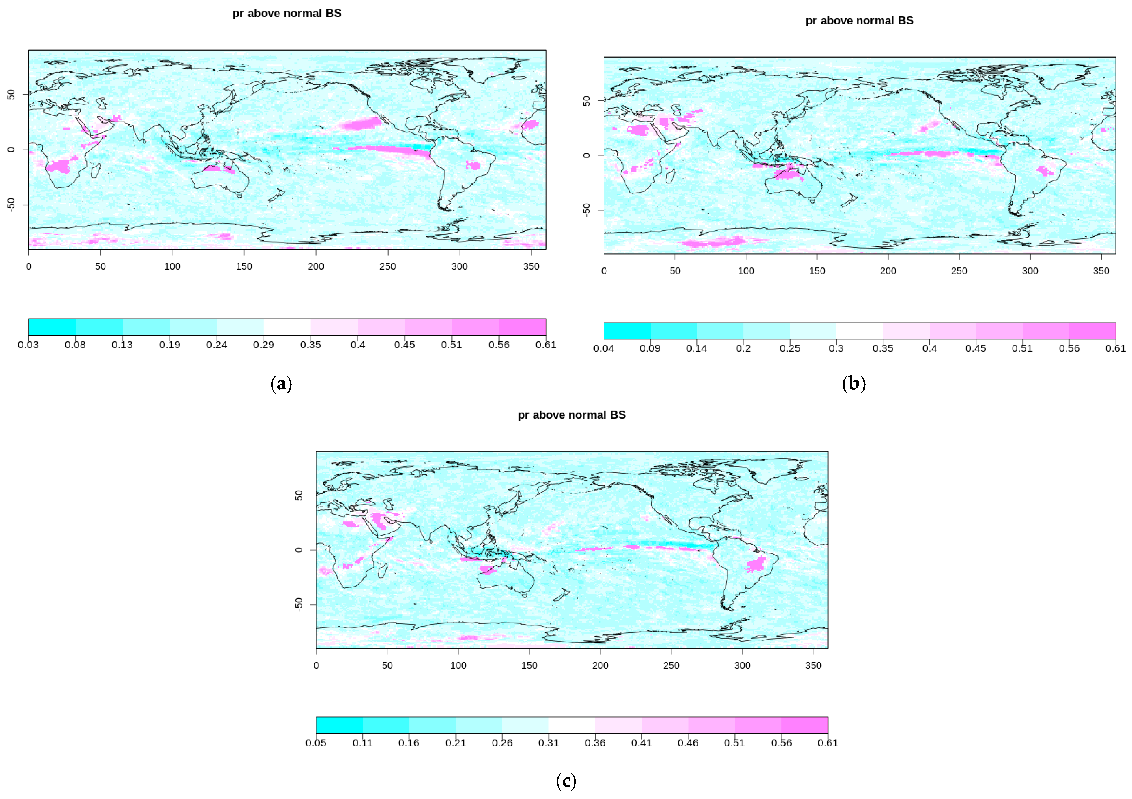
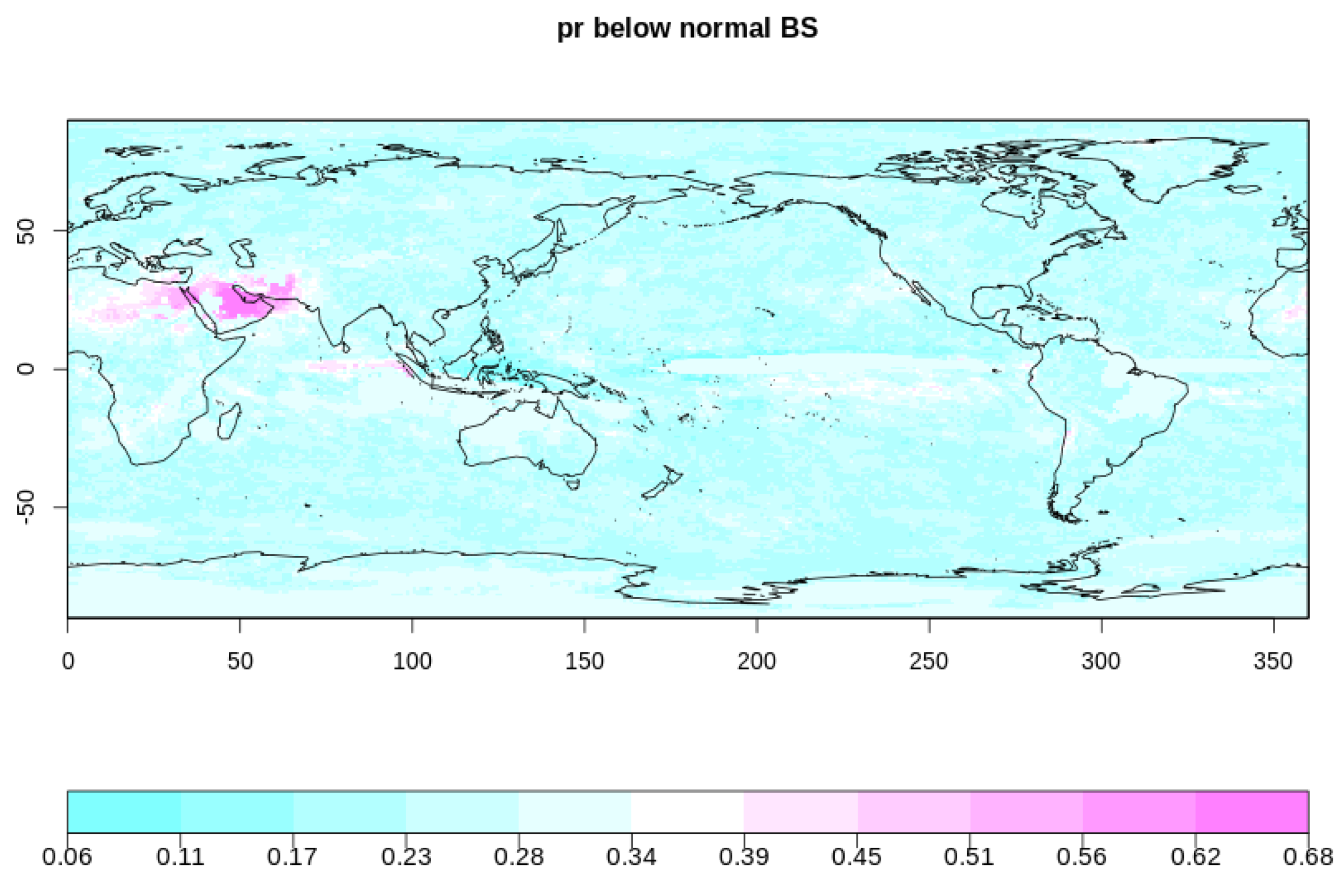
3.1. Probabilistic Evaluation of Seasonal Precipitation Hindcast

In seasonal and decadal forecasts, imperfect initial conditions and model physics and dynamics, as well as long lead time, have large impacts on the long-term mean drift in the model climate. The seasonal precipitation forecast or hindcast often has an asymptote drift, which is that the mean forecast bias is of the same sign but smaller than the long-term bias [54]. By replacing precipitation with precipitation anomaly, it partly corrects the systematic bias in the mean, for instance, the systematic difference between the climatology of the model and the observation. It also removes the trends due to aspects such as seasonal cycle, focusing on variability.

Figure 1 displays the BS spatial distribution patterns from JJA to SON, generated by Method 1. The feature of this method is that it evaluates the probabilistic accuracy of the seasonal precipitation variability, as the sample is a precipitation anomaly. Another important feature of this method is that the hindcast and the reference data share the observed TTs. To ensure a wide sample range, the climatological samples of 3 months instead of the 3-month mean were used. For TerB and TerA, the BS ranges generally fell between 0 and 0.55. The BSs greater than 0.3 (>~0.3), which are visible on the map, are distributed mostly in the tropical or sub-tropical region, and in the Antarctic. The high BS value is set to be around or more than 0.45 (>~0.45). The high BSs are found in both terciles, for TerB in particular, over the extremely dry Sahara Desert in North Africa. This indicates the probabilistic error is significant for a low precipitation forecast. The BS distribution pattern shows seasonal features in this region. Large BS (>~0.45) distribution patterns in TerA and TerB appear in JJA. As the lead time increases, they remain in JAS, and are reduced in ASO and SON. The high BS in TerB is more persistent than that in TerA. These errors may be related to the West Africa monsoon circulation. During the monsoon (June to September), the south westerly wind is strong, pushing the ITCZ northward. The very dry and hot Harmattan retreats toward the north.

Seasonal features also can be seen in the BS spatial distribution in the Arabian Peninsula, which is also a desert region. A high BS in JJA and JAS gradually reduces, and it reaches the minimum in SON. For TerB, a high BS remains even in SON. This is possibly related to the subsidence of the Indian summer monsoon flow during June to September [55], which superimposes on the impact of ENSO. In the southwest of the peninsula, a north–south-oriented mountain range (>1500 m) is bordering the Red Sea. It plays an important role in uplifting the Indian monsoon flow from the Red Sea [56] to produce heavy precipitation [57]. The recent study identifies that the large biases exist in daily maximum and minimum land surface temperatures in North Africa and the Arabian Peninsula [58]. The under-estimation can have a direct impact on latent and sensible heat fluxes and their feedback from the atmosphere, leading to too-low moisture transport and precipitation in arid regions. The precipitation rates for these two regions from System 7 indeed have negative biases (−1 mm/day), especially in JJA and JAS, as shown by the bias chart. A low anomaly correlation coefficient (ACC) frequently appears in the region where the BS is located. Charts are available at http://seasonal.meteo.fr/content/PS-scores-cartes (accessed on 30 May 2022).

Tropical rainforests have a significant impact on precipitation due to high moisture flux exchange rates between land and atmosphere. Soil moisture is also a slow varying variable at a seasonal time scale, and acts as a low boundary forcing factor of the model. A high BS distribution pattern can be observed initially in JJA for both terciles over the tropical rainforest in the Kongo Basin, but it disappears gradually after summer. The precipitation is very low there (~100 mm monthly) during the dry season from May to September, with the lowest precipitation being in July [59]. Similar conditions also can be found near the southeast of the Amazon rainforest in South America.

The continent of the Antarctic is also extremely dry (it is technically a desert). Almost all Antarctic precipitation falls as snow. West Antarctica is mostly covered by a massive ice sheet. The greenhouse-gases-induced global warming causes strong ice loss along the area 50° W–90° W. This is possibly not totally captured by the hindcast as the BS, especially for TerA, which starts to increase in ASO in the West Antarctic. The high BS pattern expands till SON when the warm season starts in the southern hemisphere (SH).

The tropical Pacific Ocean is the main region with large probabilistic errors due to its heavy precipitation in summer. Over the Nino 1 (80°–90° W and 0°–10° S) to 3.4 region (170°–120° W and 5° N–5° S) in the eastern tropical Pacific Ocean, the potential predictability for SST forcing is highest where natural variability is comparatively low, and the atmosphere responds directly to the change in SST [21]. It is true that this region has the highest ensemble mean ACC for precipitation. Nevertheless, a high BS distribution pattern along the equator in TerA can be seen in JJA. It gradually extends to the west, and it shifts further to the Nino 3 (90°–150° W and 5° N–5°S) and 4 regions (150°–160° E and 5°N–5° S) till SON, as the heavy precipitation center is moving in the same direction. Similar conditions occur for TerB with a lower BS. Marine precipitation depends greatly on SST and the moisture flux from the ocean. As the coupled system is able to capture the SST variation quite well, e.g., high ACC (see http://seasonal.meteo.fr/content/PS-scores-cartes, accessed on 30 May 2022), discrepancies in the precipitation anomalies are possibly also associated with other tropical atmospheric and oceanic short-term forcing, which propagates eastward from the Indian Ocean or westward from the Pacific Ocean in summer. In the eastern Pacific adjacent to the west coast of the US, a high BS distribution pattern in JJA gradually disappears after JAS.

Some high BSs in TerA and TerB are found to be distributed over the northwest coast of Australia in JJA. This is a northwest cloud-bands (NWCB) active region. During the dry season (May to October) in the SH, the heaviest rain often occurs from May to July due to NWCB [60]. This is a complicated process due to the influences from multiple large-scale variability modes. High BS distribution patterns in TerA and TerB subsequently emerge over the adjacent Indian Ocean in JAS during the transition of maximum and minimum frequencies of NWCB [61], expanding over the Indian Ocean till SON. This seasonal feature and/or lead time feature is particularly strong over the tropical Indian Ocean. It is worth noticing that the equatorial Indian Ocean is the origin of the MJO [30]. This suggests that intra-seasonal precipitation anomalies should be also analyzed.

Figure 2 is the same as Figure 1 but is generated by Method 2. This method uses the 3-month mean precipitation as samples, so the reference data has a smaller sample size. The most distinct feature of Method 2 is that the hindcast and the GPCP reference data each defines their own TTs. The hindcast takes advantage of the availability of the large amount of ensemble climatological samples to define TTs. Usually, it is more likely for a large number of samples to capture the distribution of a small set of samples. It can be seen that there is a significant improvement in the BS compared to that in Figure 1. The high BS distribution patterns over land shown by Figure 1 all disappeared. This indicates that the hindcast has a very good agreement with the GPCP observation over North Africa, the Arabian Peninsula, and the West Antarctic, as well as those around the Amazon and Kongo Basin during all seasons. The evaluation Method 2 demonstrates that System 7 ensemble hindcast climatology is capable of reproducing the observed precipitation probability accurately, even under drought conditions.

Compared to Figure 1, high BSs are reduced significantly, but are still visible over the tropical oceans and oceans in SH, more clearly in TerA than in TerB. They decrease over the Nino regions and increase over the Indian Ocean with the lead time, exhibiting seasonal features as well as lead time features. The similar evolution also can be observed in Figure 1. This is because the climate variability of large-scale modes like ENSO is also seasonally dependent [21]. A few errors are persistent over the tropical Atlantic during all seasons, similar to those in Figure 1 Over the tropical western Pacific (north of Australia), errors in TerA are discerned in JJA and JAS in Figure 2 but not in Figure 1.

There are some contradictions in the distribution patterns between the BS, the bias, and the ACC over the tropical ocean, where the high BS, ACC, and bias can be seen (http://seasonal.meteo.fr/content/PS-scores-cartes, accessed on 30 May 2022). The precipitation ACC is the highest over the tropical ocean, the Pacific Ocean in particular, but the negative correlations appear below the high values over the Nino 1 to 3 regions from JJA to SON. This pattern can be found in the BS distributions generated by Method 2. Indeed, the lowest BS exists in that region too. However, the negative ACC does not show any moving features, while the high BS patterns show clear moving features for both terciles. This is partly because ACC reflects the relevancy between forecast and observed anomalies. It is calculated by all samples. The BSs for TerA and TerB zoom into the samples with high or low precipitation rates to measure how well the forecast of precipitation/anomaly frequencies is achieved. It is worth pointing out that for the BS in TerN, there are few errors in the tropical Pacific by Method 2 (not shown). It is obvious that the BS is related to the bias to some extent. However, the bias in the tropical ocean increases significantly with the lead time as the season progresses, while the BS does not. The probabilistic errors, along with the highest ACC in the JJA seasonal precipitation hindcast, are also identified over the Nino 1 to 2 regions by Johnson et al. [20], with the ECMWF’s SEAS5, using the CRPSS evaluation score.

Figure 3 is the same as Figure 2 but is created by Method 3. The only difference between Method 2 and 3 is that the hindcast in Method 3 defines its TTs by the ensemble’s mean climatological samples. Only the results in JJA are presented in Figure 3. The BS spatial distribution for TerA is very close to the pattern generated by Method 2, except the slight differences in North Africa and the Arabian Peninsula. However, the BS spatial distribution for TerB in Figure 3a is significantly different from that in Figure 2a over the arid regions. It is similar to the BS distribution pattern for TerB in Figure 1a, but the errors are larger. Method 3 also estimated some high BSs for TerA and TerB distributed over tropical oceans, for example, the high BS over the western Pacific adjacent to the northwest of Australia. Note the sample size for the hindcast is the same for Method 2 and 3, but Method 2 uses more samples to define the hindcast TTs, while the hindcast and reference in Method 3 have the same sample number to define the TTs. This implies that the BS is more sensitive to TTs than to the ensemble size, although a larger ensemble size may also affect the hindcast TTs.

Figure 4 is the same as Figure 2 but is generated by Method 4. The only difference between Method 4 and 2 is that the hindcast and the reference data in Method 4 share the TTs defined by the GPCP observations, like Method 1. Only the results in JJA are presented in Figure 4. Compared to Figure 2, the most noticeable difference is the high BS for TerB over North Africa and the Arabian Peninsula. The BS spatial distribution pattern for TerA is similar to that in Figure 2b, except for over North Africa and the Arabian Peninsula, and the slightly higher BS (~0.3) distribution pattern can be discerned. It means that the BS in TerB is more sensitive to the TTs. Compared to Figure 1, the probabilistic errors in Figure 4 grow quickly with the seasons/lead time using Method 4 (not shown), although the BS for TerA is closer or even better than that in Figure 1b in JJA.

Figure 5 is the same as Figure 2 but is generated by Method 5, in which two observation data sets were used. Only the results in JJA and SON are presented. The ensemble of the GPCP and the MSWEP observation data increases the observed climatological sample size and slightly the observed sample range, which may result in changes of the observed TTs. It is more important that one more outcome, “uncertain”, was added to the observed binary events. The BS calculation still follows its definition. The resulted BS distribution patterns for TerA and TerB are very similar. Compared to Method 2, the BS shows an overall improvement in all seasons, ranging between 0 and 0.44. The most noticeable change is that the high BS for TerA and TerB are eliminated over the Nino region in the tropical Pacific. A little high BS (>~0.36) was still visible in the tropical western Pacific adjacent to the northeast of Australia in JJA and JAS. This is possibly due to the sampling method for the hindcast in Method 2, 3, and 4. The high BS (>~0.36) distribution patterns over the Indian Ocean for TerA and TerB in JJA gradually become larger in summer, reaching the maximum till SON. This is similar to those shown by Figure 1g,h and Figure 2g,h, indicating the high BS over the Indian Ocean is insensitive to different analysis methods. This is also true for small errors over the tropical Atlantic, shown by very slight BS distributions in that region, as in Figure 1 and Figure 2. The implication of this analysis is that the ensemble hindcast may generate tercile probabilities closer to 0.5 than to 0 or 1, such as over the tropical Pacific. However, the BS spatial distributions are similar when either the GPCP or MSWEP is used as the reference (not show). Note that Method 5 may have a disadvantage to the grid which has a probability closer to 0 or 1.

Figure 6 presents the BS spatial distribution in JJA generated by Method 6. Method 6 uses 3-month precipitation anomalies as samples like Method 1, but the hindcast defines its TTs by the ensemble mean climatological samples, like Method 3. The most special feature of this method is the ensemble construction. Each ensemble member starts from a different month, rather than a fixed month May, so that more ensemble data were involved. Generally, the BS in TerB is significantly higher than that generated by other methods. Although the BS spatial distribution for TerA is similar to that in Figure 3b and Figure 4b, it is significantly higher than that in Figure 5b. This analysis demonstrates the importance of the ensemble type in the statistical model for the evaluation.

The above analyses show that the errors over the tropical land in the BS maps for TerB, and for TerA as well, were detected by Method 1, 3, 4, and 6, not by Method 2 and 5 due to the TTs effects. Errors over the tropical Pacific were detected by Method 1, 2, 3, 4, 5, and 6, as Method 5 can correct those over the Nino regions with an additional probability of 0.5 in the reference data, but not over the western Pacific (north of Australia). Those over the Indian Ocean were derived from all methods, supported by the large negative precipitation bias of System 7.

3.2. Reliability

Figure 7 is the reliability decomposed from the BS for JJA using ensemble observations (Method 5) shown by Figure 5. The overall reliability, ranging from 0 to 0.33, is more satisfactory than the corresponding BS. Locations with a high BS due to large probabilistic errors are mostly caused by low reliabilities over the tropical western Pacific and the Indian Ocean. The strong correlations between reliability and the BS are also found in the analyses using other methods (not shown). Consequently, their spatial distribution patterns are similar, such as in Figure 5a,b and Figure 7a,b. Generally, high reliability leads to a good BS, but resolution may also affect the BS. Reliability is important to an ensemble prediction system as it is crucial to an accurate forecast, as well as the predictability of the system [14].

3.3. Probabilistic Evaluation of the Intra-Seasonal Precipitation Hindcast

The analyses of the seasonal precipitation hindcast detected probabilistic errors mostly over the tropical region, in particular, over the Indian Ocean and the Pacific Ocean. Precipitation forecast in the tropical region depends significantly on ENSO at seasonal to interannual time scales. By far, ENSO is the most successfully predicted large-scale mode and a known source of predictability. This leads to the intra-seasonal probabilistic evaluation in order to improve our understanding about intra-seasonal to seasonal precipitation variations, which are dominated by large-scale nature variability modes and their interactions, such as MJO and ENSO. As shown by several recent studies, it is evident that ENSO also has influences on the subseasonal precipitation forecast [62,63].

Figure 8 is the BS spatial distribution for TerA in June, July, and August. The 23-year monthly precipitation anomalies were assessed for these three months using Method 1 as an extension of the seasonal analysis of JJA. The sample size was decreased from the 3-month data in Method 1 to the monthly data. The BS has a general increase, as it is sensitive to the sample size. In addition, this is because the intra-seasonal precipitation is more affected by short-term and random forcings, which may be difficult to capture by the dynamic model. It can be also attributed to the reduced observed climatological sample range, which determines TTs. Generally, large BSs distribute at the same locations as those in the BS maps in JJA, displayed in Figure 1a,b. They remain or diverge in the tropical region and in the subtropical eastern Pacific. Compared to the BS for the seasonal precipitation anomalies (Figure 1), a significant increase of the BS for TerA occurs over the eastern equatorial Pacific Nino 1 to 3 regions in June (Figure 8a). It gradually shifts westward to the Nino 3 to 4 regions till September. This feature manifests in the seasonal BS maps shown by Figure 1, as the heavy precipitation center displaces westward. The seasonal precipitation variability in the tropical Pacific is closely associated with ENSO activity through SST [64], while MJO is more responsible for the subseasonal precipitation variability [65]. Unlike the stationary ENSO, MJO has a slow eastward-moving character, affecting the convective processes and precipitation in the tropical Pacific. Vigaud et al. [32] found that the intra-seasonal probabilistic forecast of precipitation, assessed by RPSS, is related to La Nina and El Nino, and is significantly correlated with MJO during Asian and West Africa monsoons. Over the northwest coast of Australia and the nearby equatorial Indian Ocean, the error of the monthly hindcast for TerA persists and is stronger than that in the JJA map. It suggests that the probabilistic error in this region is possibly more related to intra-seasonal short-term forcing. Figure 9 shows the pattern of the high BS emerging over the Indian Ocean for TerB in September. This is consistent with the seasonal analysis. Note that over the tropical Indian and Pacific Ocean monsoon areas in July and August, the maximum SST zone is away from Equator. Thus, the strong SST gradients initiate the convection and cross equatorial low-level jet streams, which grow through a positive feedback process [66]. In a more recently study, tropical shallow convection is identified as one of the main sources of biases in the tropical precipitation [67].

The intra-seasonal analysis reveals that the probabilistic errors in the JJA seasonal forecast are the manifestation of the deficiency mostly in the intra-seasonal forecast for June, July, and August, such as over the equatorial oceans. The decrease of forecast sample size may also have an impact on the BS.

3.4. Quantification of Uncertainties by Confidence Intervals

The uncertainty of the averaged BS over the entire tropical region (30° S–30° N and 0°–360°) was quantified by the CI95%, as more errors indicated by higher BSs were detected there. The CI95%s was initially estimated by the resampling approach for the relative comparisons of the different methods. Although the averaged BS estimated by Method 5 is the best, mostly due to the ensemble of the two observation data sets, it has a larger CI95% than that for the BSs by other methods, such as Method 2. The results for the averaged BSs in JJA are displayed in

Table 2. The CI95%, lower (LB) and upper (UB) bounds, and the percentage of the mean, calculated using the bootstrap resampling approach, are displayed for the relative comparison of Method 2 and 5. The analytical approach was applied for the Brier scores by Method 1, 2, and 3, averaged over the tropical region (30° S–30° N) in JJA. TerB and TerA represents the below- and above-normal terciles.

	resampling
TerB	forecast mean	bootstrap	CI95% LB	CI95% UB	CI95%	%
Method 2	0.2122	0.2242	0.1808	0.2656	0.0848	39.96%
Method 5	0.1398	0.1517	0.1174	0.185	0.0676	48.35%
TerA
Method 2	0.2356	0.248	0.2021	0.2915	0.0894	37.95%
Method 5	0.1521	0.1644	0.1283	0.1992	0.0709	46.61%
	method of moments
TerB	forecast mean		CI95% LB	CI95% UB	CI95%	%
Method 1	0.25		0.2423	0.2578	0.0155	6.20%
Method 2	0.2122		0.1914	0.233	0.0416	19.60%
Method 3	0.2523		0.2339	0.2708	0.0369	14.63%
TerA
Method 1	0.2451		0.2377	0.2526	0.0149	6.08%
Method 2	0.2356		0.2146	0.2566	0.042	17.83%
Method 3	0.2374		0.2168	0.258	0.0412	17.35%

under “the bootstrap resampling approach”. The analytical approach with a non-central moment estimator [13] was then applied to the accurate estimations of the CI95% for the BSs by Method 1, 2, and 3. Table 2 also lists the CI95%s for the averaged BSs over the entire tropical region in JJA, estimated by the method of moments. Using the extended analytical approach (see Equations (A5)–(A8)) for Method 5 with the observation x being uncertain, the CI95% for the BS is smaller than that estimated by the bootstrap approach (~25%). Since Method 4 uses observed TTs and precipitation as samples, it is similar but less favored than Method 1. While Method 6 produces the highest BS for TerB, it has less possibilities to be applied for the evaluation.

The CI95% for the BS in JJA, estimated by Method 1, is the highest at about 6% of the forecast mean. This is partly because the precipitation anomalies were bias-corrected to minimize the difference between the hindcast and the observation, so that the spread of its BS is narrower. It may be also because the confidence interval is disproportional to the sample size. The number of the samples used in Method 1 are three times more than those applied in Method 2 and 3. The BS estimated by Method 3 has a better CI95% than the one for the BS by Method 2 for both TerA (14.6% vs. 19.6%) and TerB (17.4% vs. 17.8%). Since the sample size of the ensemble hindcast is the same for Method 2 and 3, the difference is caused by TTs only.

With 80 drawings, the resampling approach generated bootstrap mean BS is too higher than the forecast mean BS. Experiments were performed to test the effects of different sample sizes and the total numbers of resampling. The CI95% changes very little when the bootstrap resampling increased more than 80 times. The CI95% can be calculated with much simplicity by the analytical approach with a moment estimator [13]. The samples of the BS are assumed to be normally distributed according to the central limit theorem, with the critical value of the t distribution at a significance level of 0.05 because of the unknown true standard deviation.

Table 3. The averaged CI95%s, lower (LB) and upper (UB) bounds, and percentage of the mean, estimated by the analytical approach for the seasonal evaluation of the Brier score (Method 2), over the entire tropical region (30° S–30° N). TerB and TerA represents the below- and above-normal terciles.

TerB	Forecast Mean	CI95% LB	CI95% UB	CI95%	%
MJJ	0.2018	0.1811	0.2224	0.0413	20.46%
JJA	0.2122	0.1914	0.233	0.0416	19.60%
JAS	0.216	0.1953	0.2366	0.0413	19.12%
ASO	0.2168	0.1967	0.2369	0.0402	18.54%
SON	0.2132	0.1939	0.2326	0.0387	18.15%
TerA
MJJ	0.225	0.2033	0.2468	0.0435	19.33%
JJA	0.2356	0.2146	0.2566	0.042	17.83%
JAS	0.2399	0.219	0.2609	0.0419	17.47%
ASO	0.2415	0.2211	0.2619	0.0408	16.89%
SON	0.239	0.2194	0.2586	0.0392	16.40%

lists the CI95%s for the averaged BS estimated by Method 2 over the tropical region. The CI95%s for all seasons were calculated by the analytical approach. The averaged values of the CI95% in TerB and TerA are very close to each other, about 0.04. Converting the absolute value to the percentage of the mean BS, TerA has better CI95%s (16–18%) than TerB does (18–19%) for all seasons. It is interesting to see that the CI95% decreases with the lead time, while the hindcast mean BS increases with the lead time till ASO, then it drops slightly down in SON. For TerA and TerB, the mean BS in SON achieves the best CI95%s: 0.0392 or 16.4% and 0.0387 or 18.15%, respectively. The evolution of the mean BS shows that the probabilistic errors are affected by strong seasonal features of large-scale modes like ENSO, which is strong from November to January. This is consistent with previous analysis for the BS spatial distribution. The changes in the mean BS and its CI95% with the lead time are different. There is no simple and direct relationship between the mean BS and CI95% over the tropical region.

4. Conclusions

The probabilistic evaluation in terms of accuracy and reliability was performed for 23 year (1993–2015) seasonal precipitation re-forecast, from May to November, using the BS and its decomposition. The re-forecast was produced by the Meteo-France operational seasonal forecasting system 7, with 25 ensemble members, perturbed model dynamics and initial conditions. This is a new evaluation score, in addition to the existing deterministic metrics for the seasonal and intra-seasonal forecast products.

The BS was estimated based on tercile probabilities using the non-parametric counting estimator, with the GPCP observation data as the reference. Six analyses for the seasonal hindcast were carried out to assess the robustness of the evaluation score. It is found that BS spatial distributions change significantly with sampling methods, TTs, reference data, and ensemble types. The 3-month mean precipitation and 3-month precipitation anomalies were used as samples. TTs were determined for the hindcast by (1) observed climatological samples, (2) hindcast ensemble climatological samples, (3) and hindcast mean ensemble climatological samples, for the reference by (1) the GPCB climatological samples (2), the ensemble of GPCP, and MSWEP ensemble climatological samples. The ensembles were formed by both single- and multiple-month initializations. The analysis results show that the significant probabilistic errors indicated by high BSs in TerB, and some in TerA over the dry regions, such as North Africa, the Arabian Peninsula, the Antarctic, Kongo Basin, South America, and Australia, can be corrected by taking hindcast ensemble climatological samples. Large errors, especially for TerA over the tropical ocean, were detected by all analyses. Those over the Nino region in the Pacific Ocean can be reduced in the same way. The errors over the tropical Pacific Ocean/Indian Ocean generally decrease/increase with lead time, respectively, showing seasonal and/or lead time features. The ensemble of observation data can significantly reduce the overall BS, in particular, over the tropical ocean, except over the western Pacific. This analysis method creates a new outcome, “uncertain”, for the precipitation events so that the BS is reduced. It implies that the tercile probability from the ensemble hindcast is often closer to 0.5 than either 0 or 1. Under such a condition, the increase of ensemble size is not very effective. However, the increase of BS to the maximum in SON over the tropical Indian Ocean can be seen even with different analysis methods. A few small errors persist over the Atlantic Ocean.

The intra-seasonal analysis reveals that the BS spatial distribution patterns in the intra-seasonal precipitation hindcast are similar to those in the seasonal hindcast, but the BSs are higher partly due to reduced sample size. This is also possibly related to MJO and tropical shallow convection, which can be improved by the implementation of a more sophisticated physics algorithm and the improved ensemble initial conditions for the ocean, as well as the high-resolution model configuration. The high BS patterns are mostly manifested in the JJA seasonal hindcast, except those over northwest Australia, which can be eliminated in the seasonal analysis when the sample size was increased and TTs were changed.

Since there are more probabilistic errors in the tropical region, and they change significantly with the analysis methods, the CI95% was used to quantify the uncertainty for the averaged BS over the entire tropical region. The CI95% was initially estimated by the bootstrap resampling approach for relative comparisons. Note that it is not an accuracy estimation. The CI95% was further estimated by the analytical approach of the moment estimator, which was extended to cases of non-binary outcomes and non-Bernoulli random variables. The BS calculated by Method 1 is generally the highest, but the CI95% is about 6–7% of the mean BS. The BS calculated by Method 2 was improved, but the CI95% is about 17–19% of the mean. The BS calculated by Method 3 has a relatively higher BS compared to that calculated by Method 2, but the CI95% is better, about 14–17% of the mean BS. For Method 5, the CI95%s for the averaged BS is not comparable to that calculated by Method 1, though the estimated BS is the lowest.

The averaged BS and its CI95% are not linearly correlated. The CI95% was subsequently estimated using an analytical approach for the averaged BS by Method 2 in MJJ, JJA, JAS, ASO, and SON. The CI95% is around 0.03–0.04, about 16–19% of the forecast mean, which decreases with the lead time. However, the averaged BS does not change linearly with the lead time. Generally, the BS varies with different analysis methods, and CI95% changes accordingly. However, the impact of the sample and sample size on the confidence interval should not be neglected. The increase of forecast ensemble members will certainly affect the confidence level.

To enhance the reliability of the forecast products, to provide more objective evaluations, and to detect the forecast system deficiencies, it is necessary to reduce the uncertainties in the evaluation method. As the uncertainty in the statistic model is quite large, in the future, this kind of assessment should also be applied to other evaluation scores, including the forecast skill score and the relative operative characteristic (ROC).

References

1. Ceglar, A.; Toreti, A. Seasonal climate forecast can inform the European agricultural sector well in advance of harvesting. NPJ Clim. Atmos. Sci. 2021, 4, 42. [Google Scholar] [CrossRef]
2. Miller, S.; Mishra, V.; Ellenburg, W.L.; Adams, E.; Roberts, J.; Limaye, A.; Griffin, R. Analysis of a short-term and a seasonal precipitation forecast over Kenya. Atmosphere 2021, 12, 1371. [Google Scholar] [CrossRef]
3. Osgood, D.E.; Suarez, P.; Hansen, J.; Carriquiry, M.; Mishra, A. Integrating Seasonal Forecasts and Insurance for Adaptation among Subsistence Farmers: The Case of Malawi. In Policy Research Working Paper, No. 4651; World Bank: Washington, DC, USA, 2008. [Google Scholar]
4. Daron, J.D.; Stainforth, D.A. Assessing pricing assumptions for weather index insurance in a changing climate. Clim. Risk Manag. 2014, 1, 76–91. [Google Scholar] [CrossRef] [Green Version]
5. Kharin, V.V.; Boer, G.J.; Merryfield, W.J.; Scinocca, J.F.; Lee, W.S. Statistical adjustment of decadal predictions in a changing climate. Geophys. Res. Lett. 2012, 39, L19705. [Google Scholar] [CrossRef]
6. Batte, L.; Dorel, L.; Ardilouze, C.; Gueremy, J.F. Documentation of the METEO-FRANCE Seasonal Forecasting System 7. 2019. Available online: 2018/C3S_330_Meteo-France/SC1 (accessed on 30 May 2022).
7. Brier, G.W. Verification of forecasts expressed in terms of probability. Mon. Weather Rev. 1950, 78, 1–3. [Google Scholar] [CrossRef]
8. Wilks, D. Statistical Methods in the Atmospheric Sciences; Academic Press: Cambridge, MA, USA, 2006; 627p. [Google Scholar]
9. Murphy, A.H. A new vector partition of the probability score. J. Appl. Meteor. 1973, 12, 595–600. [Google Scholar] [CrossRef] [Green Version]
10. Kharin, V.V.; Zwiers, F.W. Improved seasonal probability forecasts. J. Clim. 2003, 16, 1684–1701. [Google Scholar] [CrossRef]
11. Tippett, M.; Barnston, A.G.; Robertson, A.W. Estimation of seasonal precipitation tercile-based categorical probabilities from ensembles. J. Clim. 2007, 20, 2210–2228. [Google Scholar] [CrossRef] [Green Version]
12. Roeckner, E.; Arpe, K.; Bengtsson, L.; Christoph, M.; Claussen, M.; Dümenil, L.; Esch, M.; Giorgetta, M.; Schlese, U.; Schulzweida, U. The atmospheric general circulation model ECHAM-4: Model description and simulation of present-day climate. Max Planck Inst. Meteorol. Tech. Rep. 1996, 218, 90. [Google Scholar]
13. Bradley, A.A.; Schwartz, S.S. Summary verification measures and their interpretation for ensemble forecasts. Mon. Wea. Rev. 2011, 78, 1–3. [Google Scholar] [CrossRef]
14. Tippett, M.K.; Ranganathan, M.; Heureux, M.L.; Barston, A.G.; DelSole, T. Assessing probabilistic predictions of ENSO phase and intensity from the North American Multimodel Ensemble. Clim. Dyn. 2017, 53, 7497–7518. [Google Scholar] [CrossRef] [PubMed] [Green Version]
15. Becker, A.; Van Den Dool, H. Probabilistic seasonal forecasts in the North America multimodel ensemble: A baseline skill assessment. J. Clim. 2016, 29, 3015–3026. [Google Scholar] [CrossRef]
16. Weisheimer, A.; Palmer, T.N. On the reliability of seasonal climate forecasts. J. R. Soc. Interface 2014, 11, 20131162. [Google Scholar] [CrossRef] [PubMed]
17. Brocker, J.; Smith, L.A. Increasing the reliability of reliability diagrams. Weather Forecast. 2007, 22, 651–661. [Google Scholar] [CrossRef]
18. Hersbach, H. Decomposition of the continuous ranked probability score for ensemble prediction systems. Weather Forecast. 2000, 15, 559–570. [Google Scholar] [CrossRef]
19. Wilks, D. Diagnostic verification of the climate prediction center long-lead outlooks. J. Climate 2000, 13, 2389–2403. [Google Scholar] [CrossRef]
20. Johnson, S.J.; Stockdale, T.N.; Ferranti, L.; Balmaseda, M.A.; Molteni, F.; Magnusson, L.; Tietsche, S.; Decremer, D.; Weisheimer, A.; Balsamo, G.; et al. SEAS5: The new ECMWF seasonal forecast system. Geosci. Model Dev. 2019, 12, 1087–1117. [Google Scholar] [CrossRef] [Green Version]
21. Stockdale, T.N.; Alves, O.; Boer, G.; Deque, M.; Ding, Y.; Kumar, A.; Kumar, K.; Landman, W.; Mason, S.; Nobre, P.; et al. Understanding and Predicting Seasonal-to-Interannual Climate Variability—The Producer Perspective. Procedia Environ. Sci. 2010, 1, 55–80. [Google Scholar] [CrossRef] [Green Version]
22. Palmer, T.N. Extended-range atmospheric prediction and the Lorenz model. Bull. Am. Meteorol. Soc. 1993, 74, 49–65. [Google Scholar] [CrossRef] [Green Version]
23. Lorenz, E.N. Deterministic nonperiodic flow. J. Atmos. Sci. 1963, 20, 130–141. [Google Scholar] [CrossRef] [Green Version]
24. Slingo, J.; Palmer, T. Uncertainty in weather and climate prediction. Phil. Trans. R Soc. A 2011, 369, 4751–4757. [Google Scholar] [CrossRef] [PubMed]
25. Barston, A.G.; Li, S.; Mason, S.J.; DeWitt, D.G.; Goddard, L.; Gong, X. Verification of the first 11 years of IRI’s seasonal climate forecast. J. App. Meteoro. Clim. 2010, 49, 493–520. [Google Scholar] [CrossRef]
26. Lenssen, N.J.; Goddard, L.; Mason, S. Seasonal forecast skill of ENSO teleconnection maps. Weather Forecast. 2020, 35, 2387–2406. [Google Scholar] [CrossRef]
27. Koster, R.D.; Suarez, M.J. Soil moisture memory in climate models. J. Hydrometeorol. 2001, 2, 558. [Google Scholar] [CrossRef]
28. Seneviratne, S.I.; Koster, R.D.; Guo, Z.; Dirmeyer, P.A.; Kowalczyk, E.; Lawrence, D.; Liu, P.; Mocko, D.; Lu, C.H.; Oleson, K.W.; et al. Soil moisture memory in AGCM simulations: Analysis of Global Land–Atmosphere Coupling Experiment (GLACE) data. J. Hydrometeo. 2006, 7, 1090. [Google Scholar] [CrossRef] [Green Version]
29. Esit, M.; Kumar, S.; Pandey, A.; Lawrence, D.M.; Rangwala, I.; Yeager, S. Seasonal to multi-year soil moisture drought forecasting. NPJ Clim. Atmos. Sci. 2021, 4, 16. [Google Scholar] [CrossRef]
30. Zhang, C. Madden-Julian Oscillation. Rev. Geophys. 2005, 43, 1–36. [Google Scholar] [CrossRef] [Green Version]
31. DeMotte, C.A.; Klingaman, N.P.; Woolnough, S.J. Atmosphere-ocean coupled processes in the madden Julian oscillation. Rev. Geophy. 2015, 53, 1099–1154. [Google Scholar] [CrossRef]
32. Vigaud, N.; Robertson, A.W.; Tippett, M.K.; Acharya, N. Subseasonal predictability of boreal summer monsoon rainfall from ensemble forecasts. Front. Env. Sci 2017, 5, 67. [Google Scholar] [CrossRef] [Green Version]
33. Vigaud, N.; Robertson, A.W.; Tippett, M.K. Multimodel Ensembling of subseasonal precipitation forecasts over North America. Mon. Wea Rev. 2017, 45, 3913–3928. [Google Scholar] [CrossRef]
34. Voldoire, A.; Saint-Martin, D.; Sénési, S.; Decharme, B.; Alias, A.; Chevallier, M.; Colin, J.; Guérémy, J.; Michou, M.; Moine, M.; et al. Evaluation of CMIP6 DECK Experiments with CNRM-CM6-1. J. Adv. Model. Earth Syst. 2019, 11, 2177–2221. [Google Scholar] [CrossRef] [Green Version]
35. Larson, J.; Jacob, R.; Ong, E. The model coupling toolkit: A new Fortran90 toolkit for building Multiphysics parallel coupled models. Inter. J. High Perform. Comput. Appl. 2005, 19, 277–292. [Google Scholar] [CrossRef]
36. Déqué, M.; Reveton, C.; Braun, A.; Cariolle, D. The ARPEGE/IFS atmosphere model: A contribution to the French comunitu climate modelling. Clim. Dyn. 1994, 10, 249–266. [Google Scholar] [CrossRef]
37. Noilhan, J.; Planton, S. A simple parameterization of land surface processes for meteorological models. Mon. Weather Rev. 1989, 117, 536–549. [Google Scholar] [CrossRef]
38. Voldoire, A.; Decharme, B.; Pianezze, J.; Brossier, C.L.; Sevault, F.; Seyfried, L.; Garnier, V.; Bielli, S.; Valcke, S.; Alias, A.; et al. SURFEX v8.0 interface with OASIS3-MCT to couple atmosphere with hydrology, ocean, waves and sea-ice models, from coastal to global scales. Geosci. Model Dev. 2017, 10, 4207–4227. [Google Scholar] [CrossRef] [Green Version]
39. Decharme, B.; Delire, C.; Minvielle, M.; Colin, J.; Vergnes, J.-P.; Alias, A.; Saint-Martin, D.; Séférian, R.; Sénési, S.; Voldoire, A. Recent Changes in the ISBA-CTRIP Land Surface System for Use in the CNRM-CM6 Climate Model and in Global Off-Line Hydrological Applications. J. Adv. Model. Earth Syst. 2019, 11, 1207–1252. [Google Scholar] [CrossRef]
40. Madec, G.; The NEMO Team. NEMO Ocean Engine (V3.6); Scientific Notes of Climate Modelling Center, Institute Pierre-Simon Laplace (IPSL): Guyancourt, France, 2016; ISSN 1288-1619. [Google Scholar]
41. Salas y Mélia, D. A global coupled sea ice-ocean model. Ocean. Model 2002, 4, 137–172. [Google Scholar] [CrossRef]
42. Batte, L.; Deque, M. Randomly correcting model errors in the ARPEGE-Climate v6.1 component of CNRM-CM: Application for seasonal forecasts. Geosci. Model Dev. 2016, 9, 2055–2076. [Google Scholar] [CrossRef] [Green Version]
43. Boisserie, M.; Decharme, B.; Descamps, L.; Arbogast, P. Land surface initialization strategy for a global re-forecast dataset. Q. J. Roy. Meteor. Soc. 2016, 142, 880–888. [Google Scholar] [CrossRef] [Green Version]
44. Dubois, C.; Mercator-Ocean, Toulouse, France. Initial Condition from Mercator-Ocean. Personal communication, 2016. [Google Scholar]
45. Adler, R.F.; Huffman, G.J.; Chang, A.; Ferraro, R.; Xie, P.P.; Janowiak, J.; Rudolf, B.; Schneider, U.; Curtis, S.; Bolvin, D.; et al. The Version-2 Global Precipitation Climatology Project (GPCP) Monthly Precipitation Analysis (1979–Present). J. Hydrometeorol. 2003, 4, 1147–1167. [Google Scholar] [CrossRef]
46. Beck, H.E.; van Dijk, A.I.J.M.; Levizzani, V.; Shellekens, J.; Miralles, D.G.; Martens, B.; de Roo, A. MSWEP: 3-hourly 0.25 global grided precipitation (1979–2015) by merging gauge, satellite, and reanalysis data. Hydrol. Earth Syst. Sci. 2017, 21, 589–615. [Google Scholar] [CrossRef] [Green Version]
47. Manubens, N.; Caron, L.-P.; Hunter, A.; Bellprat, O.; Exarchou, E.; Fučkar, N.S.; García-Serrano, J.; Massonnet, F.; Ménégoz, M.; Sicardi, V.; et al. An R package for climate forecast verification. Environ. Model. Softw. 2018, 103, 29–42. [Google Scholar] [CrossRef]
48. Specq, D.; Batte, L. Improving subseasonal precipitation forecasts through a statistical-dynamical approach: Application to the southwest tropical Pacific. Clim. Dyn. 2020, 55, 1913–1927. [Google Scholar] [CrossRef]
49. Efron, B. Better Bootstrap Confidence Intervals; Technical Report, No. 14; Stanford University: Stanford, CA, USA, 1984. [Google Scholar]
50. Pathak, P.K. Sufficiency in sampling theory. Ann. Math Stat. 1964, M43, 508–515. [Google Scholar] [CrossRef]
51. Pathak, P.K.; Rao, C.R. The Sequential Bootstrap. Handb. Stat. 2013, 31, 2–18. [Google Scholar] [CrossRef]
52. Bradley, A.; Schwartz, S.S.; Hasino, T. Sampling uncertainty and confidence intervals for the Briere score and Brier skill score. Weather Forecast. 2008, 23, 992–1006. [Google Scholar] [CrossRef]
53. Murphy, A.H.; Winkler, R.L. Diagnostic verification of probability forecasts. Int. J. Forecast. 1992, 7, 435–455. [Google Scholar] [CrossRef]
54. Hermanson, L.; Ren, H.L.; Velligna, M.; Dunstone, N.D.; Hyder, P.; Ineson, S.; Scaife, A.A.; Smith, D.M.; Thomson, V.; Tian, B.; et al. Different types of drifts in two seasonal forecast systems and their dependence on ENSO. Clim. Dyn. 2018, 51, 1411–1426. [Google Scholar] [CrossRef] [Green Version]
55. Attada, R.; Dasari, H.P.; Parekh, A.; Chowdary, J.S.; Langodan, S.; Knio, O.; Hoteit, I. The role of the Indian summer monsoon variability on Arabian Peninsula summer climate. Clim. Dyn. 2018, 52, 3389–3404. [Google Scholar] [CrossRef]
56. Chakraborty, A.; Behera, S.K.; Mujumdar, M.; Ohba, R.; Yamagata, T. Diagnosis of tropospheric moisture over Saudi Arabia and influences of IOD and ENSO. Mon. Weather Rev. 2006, 134, 598–617. [Google Scholar] [CrossRef]
57. Almazroui, M. Sensitivity of a regional climate model on the simulation of high intensity rainfall events over the Arabian Peninsula and around Jeddah (Saudi Arabia). Theor. Appl. Climatol. 2011, 104, 261–276. [Google Scholar] [CrossRef] [Green Version]
58. Xu, Y. Global Root Zone Soil Moisture: Assimilation and Impact; CNRM, Meteo-France: Toulouse, France, 2022; (To be submitted). [Google Scholar]
59. Juarez, R.I.N.; Li, W.; Fu, R.; Fernandes, K.; Cardoso, A.D.O. Comparison of Precipitation Datasets over the Tropical South American and African Continents. J. Hydrometeorol. 2009, 10, 289–299. [Google Scholar] [CrossRef]
60. Telcik, N.; Pattiaratch, C. Influence of Northwest Cloudbands on Southwest Australian Rainfall. J. Climatol. 2014, 2014, 671394. [Google Scholar] [CrossRef] [Green Version]
61. Reid, K.J.; Simmonds, I.; Vincent, C.; King, A.D. The Australia northwest cloudband: Climatology, mechanisms, and association with precipitation. J. Clim. 2019, 32, 6665–6684. [Google Scholar] [CrossRef]
62. Specq, D.; Batte, L.; Deque, M.; Ardilouze, C. Multimodel forecasting of precipitation at subseasonal timescales over the Southwest tropical Pacific. Earth Space Sci. 2020, 7, e2019EA001003. [Google Scholar] [CrossRef]
63. Andrade, F.M.D.; Coelho, C.A.S.; Cavalcanti, I.F.A. Global precipitation hindcast quality assessment of the subseasonal to seasonal (S2S) prediction project models. Clim. Dyn. 2018, 52, 5451–5475. [Google Scholar] [CrossRef]
64. Yun, K.-S.; Lee, J.-Y.; Timmermann, A.; Stein, K.; Stuecker, M.F.; Fyfe, J.C.; Chung, E.-S. Increasing ENSO–rainfall variability due to changes in future tropical temperature–rainfall relationship. Commun. Earth Environ. 2021, 2, 43. [Google Scholar] [CrossRef]
65. Recalde-Coronel, G.C.; Zaitchik, B.; Pan, W.K.Y. Madden-Julian Oscillation influence on sub-seasonal rainfall variability on the west of South America. Clim. Dyn. 2020, 54, 2167–2185. [Google Scholar] [CrossRef]
66. Sabin, T.P.; Babu, C.A.; Joseph, P.V. SST-convection relationship over tropical oceans. Int. J. Climatol. 2012, 33, 1424–1435. [Google Scholar] [CrossRef] [Green Version]
67. Good, P.; Chadwick, R.; Holloway, C.E.; Kennedy, J.; Lowe, J.A.; Roehig, R.; Rushley, S.S. High sensitivity of tropical precipitation to local sea surface temperature. Nature 2020, 589, 408–414. [Google Scholar] [CrossRef]
Figure 1. The spatial distribution of the Brier score for the seasonal hindcast of precipitation anomalies based on the terciles determined by the GPCP observation (Method 1). From top, each row represents the Brier scores for the below, (a,c,e,g), and the above₋normal terciles, (b,d,f,h), at lead times of 1, 2, 3, and 4 months, corresponding to JJA, JAS, ASO, and SON, respectively.
Meteorology 01 00016 g001aMeteorology 01 00016 g001b
Figure 2. The spatial distribution of the Brier score for the seasonal hindcast of a 3₋month mean precipitation, using the hindcast tercile thresholds determined by the ensemble climatology (Method 2). The reference is the GPCP observations. The Brier scores for the below, (a,c,e,g), and the above₋normal terciles, (b,d,f,h), at 1, 2, 3, and 4 lead months correspond to JJA, JAS, ASO, and SON, respectively.
Meteorology 01 00016 g002aMeteorology 01 00016 g002b
Figure 3. The spatial distribution of the Brier scores for the seasonal hindcast of a 3₋month mean precipitation in JJA, using the hindcast tercile thresholds derived from the ensemble mean climatological samples, with the GPCP data as references (Method 3). The Brier scores for the below (a) and the above₋normal terciles (b) at 1 lead month correspond to JJA.
Meteorology 01 00016 g003
Figure 4. The spatial distribution of the Brier scores for the seasonal hindcast of a 3-month mean precipitation in JJA, using the hindcast tercile thresholds derived from the GPCP climatological samples (Method 4). The Brier scores for the below (a) and the above₋normal terciles (b) at 1 lead month correspond to JJA.
Meteorology 01 00016 g004
Figure 5. The spatial distribution of the Brier score for the seasonal hindcast of precipitation using the GPCP and the MSWEP ensemble observation as the reference data (Method 5). The Brier scores for the below, (a,c), and the above₋normal terciles, (b,d), at lead times of 1 and 4 months correspond to JJA and SON, respectively.
Meteorology 01 00016 g005
Figure 6. The spatial distribution of the Brier scores for the 3₋month precipitation anomalies in JJA, using the tercile thresholds for the hindcast derived from ensemble mean climatological samples, with a mixed month initialization ensemble (Method 6). The Brier scores for the below (a) and the above₋normal terciles (b) at 1 lead month correspond to JJA.
Meteorology 01 00016 g006
Figure 7. The reliability decomposed from the Brier score for precipitation in JJA using the GPCP and the MSWEP ensemble observation as the reference, in the above₋normal (a) and the below₋normal terciles (b).
Meteorology 01 00016 g007
Figure 8. The evaluation of the monthly precipitation anomalies (1993–2015) by the Brier score in the above₋normal terciles using the GPCP observed tercile thresholds. The spatial distributions for June, (a), July, (b), and August, (c), are displayed.
Meteorology 01 00016 g008
Figure 9. Same as Figure 8 but for the below₋normal tercile in September.
Meteorology 01 00016 g009