1. Introduction
Over the past 150 years, atmospheric methane (CH
4) concentrations have more than doubled, significantly contributing to climate change [
1]. Mitigating CH
4 emissions, due to its short atmospheric lifetime compared to carbon dioxide (CO
2), offers an effective strategy for short-term climate stabilization [
2], while accurate emissions measurements are crucial for assessing environmental impact, minimizing product losses, and identifying large emission sources. CH
4 emissions can be measured using top-down (TD) or bottom-up (BU) approaches [
3,
4]. TD approaches employ satellites, aircraft, drones, or ground-based instruments (fixed or mobile) to measure atmospheric CH
4 enhancements over a geographic region or a given site, inferring total emissions using various methods such as mass balance, micrometeorological techniques, inverse dispersion modeling, mobile flux plane, or tracer gas approaches. BU approaches, on the other hand, estimate emissions at regional, state, or national levels by aggregating direct measurements from individual equipment, operations, or facilities. High costs and limited source specificity constrain TD studies, while BU methods, despite providing source-specific data, face accessibility challenges in large facilities, potentially biasing facility-level emission rate (FLER) estimates [
3,
4,
5,
6].
Building on the limitations of both TD and BU approaches, recent research has highlighted the inherent complexity of CH
4 emissions from natural gas infrastructure, which further complicates accurate quantification [
3,
7]. Emissions arise from a wide range of sources, including production sites, processing plants, compressor stations, and distribution networks, each exhibiting distinct operational characteristics and regional variability [
8,
9]. This heterogeneity is compounded by the presence of disproportionately high-emitting sources, or “super-emitters,” and the temporal variability of emissions, which can lead to significant discrepancies in FLER estimates [
10,
11]. To address these challenges, a variety of measurement techniques have been developed [
12]. Static methods include eddy covariance towers and autochambers [
13], while mobile methods employ vehicle-mounted analyzers using tracer correlation methods (TCM) and cavity ring-down spectrometry (CRDS) [
4,
6,
14,
15]. small Unmanned Aerial System (sUAS) integrate technologies such as quantum cascade laser absorption spectrometer (QCLAS), active AirCore samplers, and miniaturized infrared analyzers to quantify methane emissions from diverse sources, offering high spatial resolution and adaptable flight patterns for targeted plume sampling in complex environments [
16,
17,
18]. An emerging line of research has demonstrated the use of lightweight open-path sensors, such as tunable diode laser absorption spectroscopy (TDLAS) and laser methane detectors, mounted on sUAS to detect, map, and quantify methane plumes in real time, showing promise for rapid emissions localization across complex terrain and infrastructure [
19,
20,
21]. Manned aircraft integrate technologies like flame ionization detectors (FIDs) and LiDAR for large-scale assessments [
22], whereas optical gas imaging (OGI) and airborne mass balance techniques refine urban CH
4 flux estimates [
5]. Satellite-based approaches leverage imaging spectroscopy and machine learning to enable large-scale emission monitoring [
12,
23]. Despite these advancements, traditional BU inventories often underrepresent actual emissions, underscoring the need for more spatially and temporally resolved measurement strategies [
3,
24].
One widely adopted technique for facility-level or area source CH
4 quantification is the Tracer Flux Ratio (TFR) method [
6,
25,
26,
27,
28]. This method involves the controlled release of a tracer gas at a known flow rate, strategically positioned near the target source. This proximity minimizes the need for dispersion modeling by ensuring similar atmospheric transport conditions. The TFR method is particularly advantageous because it enables accurate estimation of total facility-level CH
4 emissions without relying on meteorological measurements or complex dispersion models [
4,
15]. It is especially useful in complex environments where direct measurements are challenging.
While the TFR method offers a robust solution for quantifying CH
4 emissions in complex environments, recent advancements in sUAS-based monitoring have further expanded the toolkit for facility-level assessments [
29]. sUAS equipped with high-precision sensors can complement TFR deployments by providing flexible, high-resolution spatial coverage, especially in areas where ground-based access is limited. The effectiveness of these aerial platforms, however, is closely tied to the optimization of their flight paths [
30,
31,
32]. For example, Ref. [
31] demonstrated that standardized and strategically designed sUAS trajectories significantly improve the accuracy of CH
4 quantification during field campaigns in Alberta. Similarly, Ref. [
30] found that flight path variations can greatly influence detection sensitivity at compressor stations, underscoring the importance of trajectory planning in capturing spatial emission variability. Further innovations by [
33] in 3D path planning have shown promise in navigating complex terrains, enhancing data completeness and reducing uncertainty. Ref. [
32] further emphasizes the versatility of sUAS in high-density spatial mapping and hazard detection, noting that the ability to capture volumetric emissions data enables a more precise understanding of facility-specific emissions profiles—an advancement with direct implications for shaping regulatory frameworks aimed at reducing greenhouse gas impacts. These developments highlight the growing role of sUAS not only as standalone measurement tools but also as integral components of hybrid monitoring strategies that combine different quantification methods with sUAS sensing to achieve more comprehensive and reliable emissions assessments.
Discrepancies and frequent underestimations in CH
4 emission measurements from oil and gas facilities, whether using TD or BU approaches [
3,
12], can be mitigated by improving the accuracy and frequency of emission measurements, capabilities that recent advancements in sUAS based sensing offer [
12,
29,
34]. sUAS offers unique advantages, including unrestricted access to road-inaccessible areas, high-resolution measurements at lower altitudes than manned aircraft, cost efficiency, and the ability for frequent deployment to capture temporal variations in emissions [
35,
36]. Their use in monitoring CH
4 emissions offers a significant advantage over traditional methods by enabling more detailed assessments, informing and facilitating continuous monitoring, and providing real-time data on emission variations across different times and locations due to their ease of deployment and maneuverability [
29,
37,
38]. In this study, we apply the TFR method using sUAS to assess CH
4 emissions at natural gas facilities, focusing on optimizing flight patterns to improve quantification accuracy and operational efficiency. By enhancing downwind concentration measurements and extending sUAS battery life, optimized flight pattern offers a promising approach for achieving more precise and frequent CH
4 emissions quantification, thereby advancing current capabilities in facility-scale CH
4 monitoring.
2. Methods
2.1. Tracer Flux Ratio
The TFR method quantifies CH
4 emissions by relating its downwind concentration enhancement,
, to that of a simultaneously released tracer gas with a known release rate. This ratio-based approach eliminates the need to estimate a transport proportionality coefficient,
, which is often difficult to constrain without applying simplifying assumptions [
4,
6,
39,
40]. Here,
represents the enhancement of CH
4 concentrations observed downwind of the emission source or target facility relative to ambient background levels. The background concentration is characterized from upwind measurements taken outside of the plume influence. This approach enables identification of plume-impacted regions and supports emission quantification by focusing on areas where CH
4 is elevated above the regional background. The proportionality coefficient
is influenced by meteorological factors such as wind speed, turbulence, solar irradiance, atmospheric boundary layer height, local topography, and downwind distance. The relationship is as expressed in Equation (
1):
To bypass the need for explicitly determining
, a known tracer gas with a defined release rate,
, is introduced near the CH
4 source. The downwind concentration enhancements of both
and tracer gas
are then measured. Assuming uniform dispersion and transport conditions, the emission rate can be calculated as expressed in Equation (
2):
Previous studies suggest that TFR-based facility-level emission estimates typically exhibit uncertainties of approximately
[
6,
41,
42].
2.2. Tracer Drone System
A custom-built tracer drone system was developed to optimize high-resolution concentration measurements. The system integrates Aeris Technologies’ MIRA Strato series laser gas analyzers with the Harris Aerial Carrier H6 Electric heavy-lift hexacopter. The H6 Electric platform provides a flight time of approximately 35 min with an maximum payload, from fully charged to about 50% battery, and a maximum operational wind speed of , making it suitable for varied environmental conditions.
The MIRA Strato analyzers employ mid-infrared laser absorption spectroscopy to measure CH4, ethane (C2H6), nitrous oxide (N2O), and CO2 with reported 1-s integrated detection sensitivities of 1 ppb CH4, 500 ppt C2H6, 200 ppt N2O, and 200 ppb CO2. The analyzers operate over a concentration range of 10 ppb to 100,000 ppm with a data acquisition rate of up to 10 Hz (standard 1–2 Hz), and during field deployment, they were operated at 1 Hz resolution. To ensure minimal measurement interference, the analyzers’ sampling port was mounted approximately 40 cm below the rotor plane on a downwind-facing drone leg.
Data are collected and processed onboard a Raspberry Pi, which appends GPS coordinates and altitude metadata to each data point before transmitting them to ground control via MAVLink and LoRa communication modules. This setup enables real-time monitoring of CH
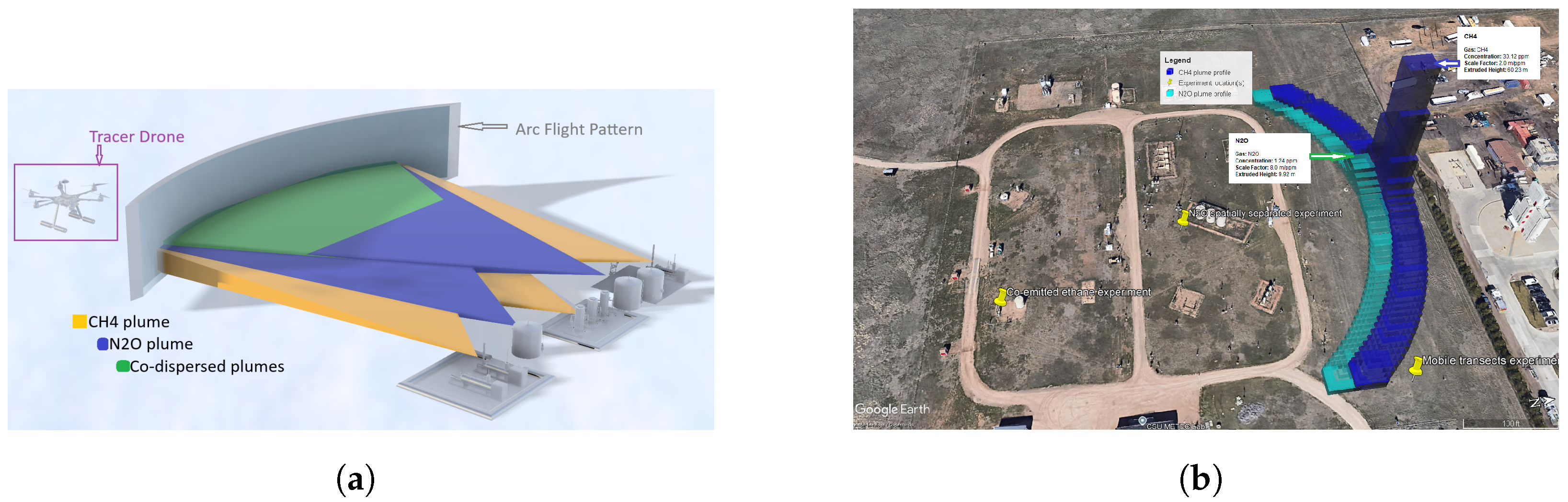
4 and tracer gas plumes and facilitates precise flight adjustments to optimize plume capture. The modeled plume from a facility with tracer release and an aerial view of the METEC facility, overlaid with gas concentration profiles for CH
4 and N
2O, are illustrated in
Figure 1. The arc sampling method was employed to capture spatial distributions of gas plumes, with CH
4 concentrations shown in blue and N
2O in green. Yellow markers denote the locations of specific experimental setups, including the co-emitted C
2H
6 experiment, N
2O spatially separated experiment, and mobile transects experiment. The curved arcs illustrate the flight paths or sampling trajectories used to detect and map the gas plumes across the facility.
Flights were conducted at altitudes ranging from 6 to 25 m above ground level (AGL), depending on the concentration boundary layer. The sUAS has a maximum speed of 15 m/s; however, during planned flight missions, it typically travels at a steady speed of 3 m/s. When operated manually by the Remote Pilot in Control (RPiC), the sUAS travels at speeds ranging from 3 to 5 m/s during plume interception maneuvers. Each flight began with an upwind transect at the highest planned altitude to characterize background concentrations, defined as stable measurements with no detectable plume enhancement. To confirm plume edges, we extended horizontal flight paths laterally until CH4 concentrations returned to background values for at least 10 consecutive seconds. This ensured that the outer edges of the flight transects captured the full lateral extent of the plume. Downwind passes were executed 40–80 m from the source, with arc radii determined from real-time wind direction to optimize coverage of the plume centerline.
This flight procedure was repeated across multiple plume transects and downwind distances to enable robust plume mapping and emission quantification.
2.3. Experimental Setup
Experiments were conducted at the Methane Emissions Technology Evaluation Center (METEC) to assess the TFR method’s accuracy under both controlled and real-world conditions. Located at Colorado State University, METEC is a unique outdoor laboratory designed to simulate realistic oil and gas facility operations, offering a controlled environment where CH4 emissions can be released from a variety of equipment types and configurations. The facility includes over 200 leak points across mock well pads, separators, tanks, and compressor stations, enabling researchers to test detection technologies under conditions that closely mimic those encountered in the field. This level of realism is critical for evaluating the performance of emission quantification methods like TFR, as it allows for systematic testing across a range of environmental variables and operational scenarios. By validating measurement techniques at METEC prior to field deployment, researchers can identify potential limitations, refine methodologies, and improve confidence in emissions data collected from actual oil and gas facilities. Three experimental configurations were implemented to assess TFR performance under ideal and non-ideal tracer-source alignment scenarios:
Natural Gas Release with Co-Emitted Ethane as Tracer: In this setup, whole natural gas was released from a point source, with C2H6 acting as a co-emitted tracer gas. Since C2H6 is naturally present in the gas mixture and emitted simultaneously with CH4, this configuration satisfies key TFR assumptions regarding spatial and temporal co-location of tracer and target gases. The whole gas release averaged (standard liters per minute, referenced to 25 °C and 1 atm, per Alicat flow controller specifications), with CH4 contributing and C2H6 contributing , as determined from gas chromatography (GC) analysis.
Controlled Release of Methane and Separate Nitrous Oxide Tracer: A second configuration involved controlled releases of CH4 paired with N2O as an externally released tracer gas. Measurements were taken at sufficiently long downwind distances to promote plume mixing and co-dispersion, simulating less ideal but more realistic field conditions where tracer and target sources are not spatially coincident. In the controlled release experiment, CH4 and N2O were released at identical rates of and , respectively, as in the natural gas release with co-emitted C2H6 as tracer.
Separated Tracer and Emission Source Configuration: A third experimental configuration examined the performance of the TFR method when the tracer gas N2O was released from a location spatially offset from the CH4 emission source. CH4 was released from the thief hatch of a storage tank at a height of approximately 5.2 m, while N2O was released from a gas cylinder positioned roughly 8 m away horizontally, with a release height of approximately 3 m. Concentration measurements were collected at downwind distances closer to the release points (<60 m) than in the co-dispersion case, with sUAS flying pre-programmed curtain and arc patterns. This setup was designed to test the sensitivity of sUAS-based sampling strategies and concentration ratio estimation approaches under non-ideal conditions. Two different CH4 release rates were used: and . The tracer release rate remained constant at for both CH4 release conditions.
A summary of the controlled CH
4 emission experiments and tracer configurations is provided in
Table 1. These configurations were designed to systematically evaluate the sensitivity of the TFR method to tracer gas selection and spatial alignment with the emission source. The first setup, in which CH
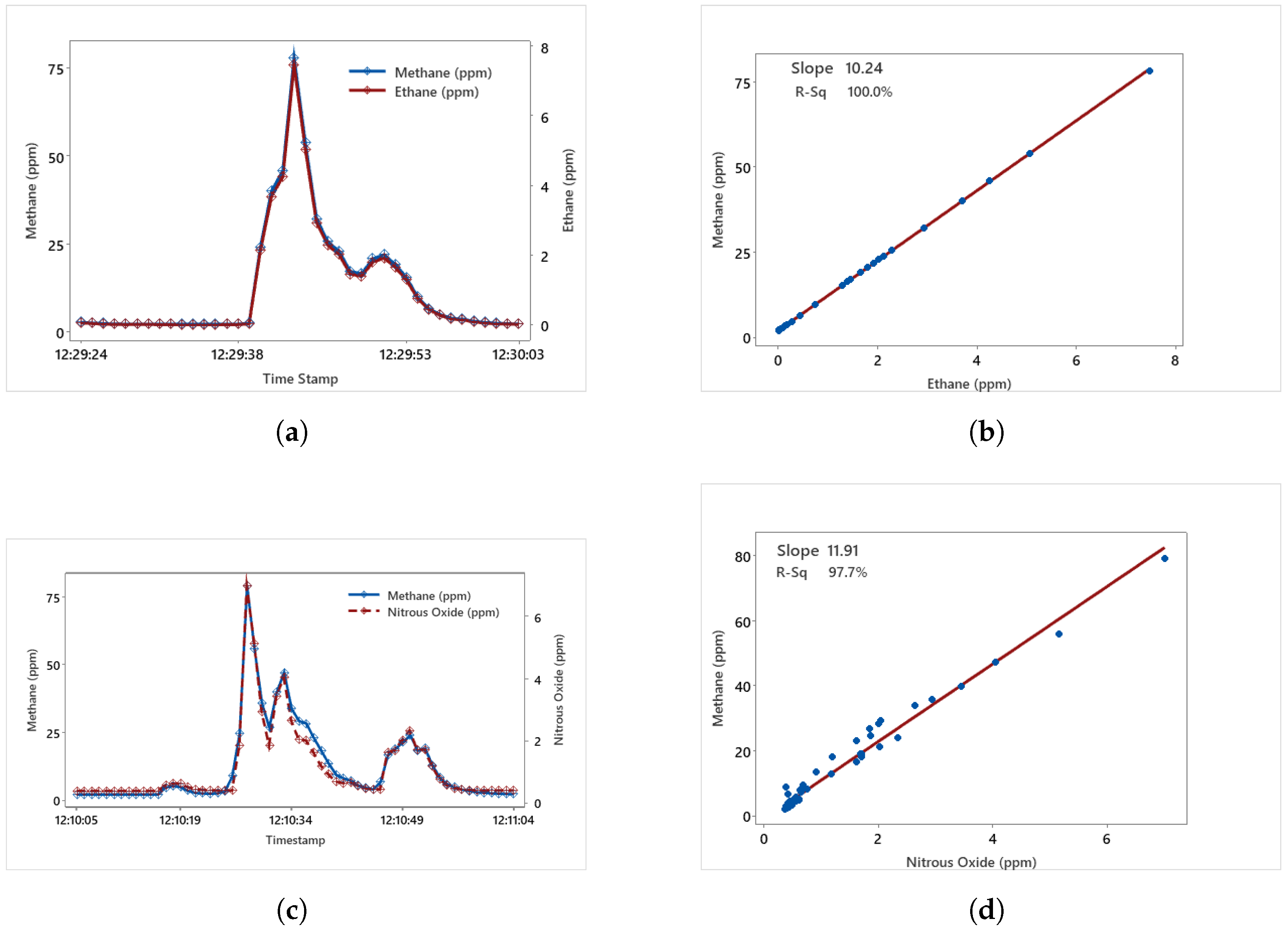
4 and the tracer gas were co-emitted from the same point, serves as a controlled benchmark for method accuracy under ideal conditions. While this configuration is not representative of typical field deployments, where tracer gases and emission sources are rarely co-located, it provides a lower-bound estimate of uncertainty and highlights the method’s potential under optimal conditions. Comparisons across all configurations allow for a robust assessment of how deviations from ideal tracer-source alignment affect quantification accuracy and uncertainty. These dynamics are illustrated in
Figure 2, which presents time series and regression plots for both the natural gas configuration with co-emitted C
2H
6 and the controlled CH
4 release with a separate N
2O tracer.
2.4. Flight Pattern Optimization
To maximize spatial resolution and capture CH4 concentration gradients effectively, we investigated the impact of flight pattern on TFR-based quantification. Traditional mobile transect methods, such as vehicle-mounted sensors, are limited in their ability to resolve vertical and lateral plume structure, particularly for elevated emission sources. Two primary flight patterns were evaluated:
Curtain Pattern: The tracer drone executes multiple horizontal passes at multiple altitudes perpendicular to the wind direction to construct a vertical cross-sectional concentration profile of the plume.
Arc Pattern (Proposed Optimization): The tracer drone follows a semi-circular arc at a fixed downwind distance and varying heights, aligning with the expected Gaussian dispersion of the plume to cover the concentration boundary layer.
The arc pattern was introduced to provide a more accurate approximation of the plume’s true spatial structure, improving quantification accuracy by ensuring uniform sampling across the plume width. Additionally, this method mitigates uncertainties related to variable wind conditions and non-uniform CH
4–tracer co-dispersion, particularly from elevated sources such as vents and exhaust stacks, because of the ability to sample at varying height using sUAS. The arc pattern can effectively cover shifts in plume width due to changing wind directions, as long as the wind does not shift by more than 20 degrees.
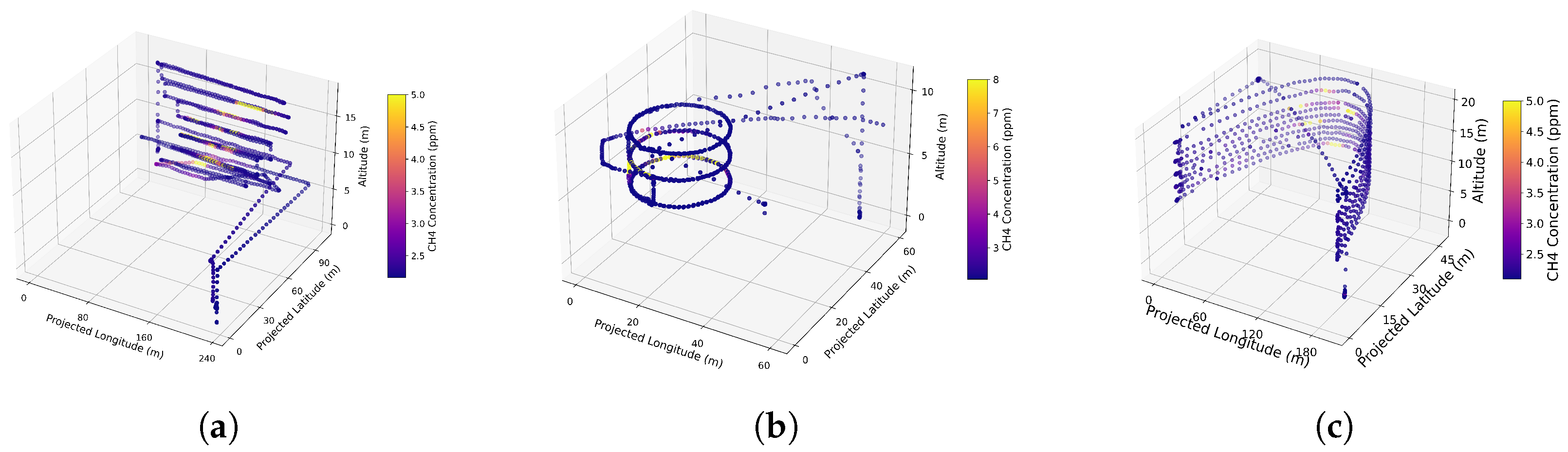
Figure 3 illustrates the curtain, cylindrical, and arc flight patterns.
The flight path optimization addresses a key limitation of sUAS-based methods: the conflict between battery duration and payload weight. By using an arc flight pattern instead of a cylindrical one, which primarily addresses plume lateral dispersion and shifting wind, battery life is improved, allowing for more extensive plume measurements. Rather than capturing the plume’s normal distribution through a control volume analysis with a cylindrical pattern, we have introduced a control surface analysis using the arc flight pattern [
34]. The CH
4 and tracer gas plumes are traversed multiple times (more than 10) to minimize measurement variability. The simultaneous rise, peak, and fall times of the target and tracer gases indicate adequate mixing and are used to assess measurement quality.
2.5. Methane-to-Tracer Concentration Ratios Estimation
Several methodologies exist for estimating the CH
4-to-tracer gas ratio from downwind concentration data [
4,
6,
39,
42,
43,
44]. Studies have moved beyond the standard slope method and single tracer release by employing multiple approaches, such as integrated inverse-dispersion and dual analysis techniques, respectively, to capture plume variability without solely relying on a linear slope [
4,
45]. We evaluated the following approaches as in [
42]:
Plume Integration: The total integrated area of the CH4 and tracer plumes is used to compute their ratio.
Peak Height Ratio: The maximum observed concentrations of CH4 and tracer gas are used to determine their ratio.
Scatter Plot Regression: A linear regression is performed on the scatter plot of measured CH4 and tracer concentrations.
Gaussian Plume Model: CH4 emissions are estimated using a Gaussian dispersion model.
Each method has distinct advantages and limitations. Plume integration minimizes sensitivity to incomplete mixing, while peak height ratio is robust to background variability [
42]. Scatter plot regression provides a statistical basis for ratio estimation but assumes fully mixed plumes [
42]. The Gaussian model approach incorporates atmospheric transport dynamics but requires precise meteorological input [
4,
42]. Various methods for analyzing downwind tracer plumes to estimate facility-level CH
4 emission rates using dual tracer gases to simulate emission sources have been outlined by [
4]. These methods include dual correlation, dual area analysis, single correlation, and linear combination of tracer plumes. Dual correlation involves plotting concentrations of overlapping plumes and performing linear regression to determine emission rates. Dual area analysis integrates plume areas when spatial overlap is insufficient. Single correlation is used when CH
4 correlates strongly with only one tracer. Linear combination uses a mix of tracers for intermediate-distance transects. Each method has specific criteria for plume acceptance based on correlation coefficients and tracer ratios [
4].
2.6. Data Analysis and Emission Rate Estimation
Downwind plume profiles were acquired using a tracer drone flown through the concentration boundary layer at the METEC facility. Data were collected via two dynamic flight patterns, curtain and arc, as well as stationary hovering within the plume for 1–3 min. These sampling strategies enabled a comparative analysis of spatial plume coverage and concentration gradients under real-world dispersion conditions.
Emission rates were estimated using the TFR methodology with two distinct tracer gas configurations:
Ethane, co-emitted from a whole gas release, served as the tracer gas for benchmark scenarios. Because C2H6 and CH4 originate from the same emission source in this configuration, it satisfies the spatial and temporal co-location requirements of TFR. This setup represents an ideal scenario, establishing a lower-bound estimate of TFR uncertainty attributable to atmospheric variability and flight sampling strategy, rather than tracer-source separation or gas dissimilarity.
Nitrous oxide was deployed as an independent tracer in controlled methane release experiments. This configuration introduces controlled spatial separation between tracer and target emissions and is used to evaluate the additional uncertainty introduced by tracer deployment geometry and gas-specific dispersion properties.
Multiple downwind plumes were sampled under varying meteorological conditions to enhance statistical robustness. For each plume encounter, CH
4-to-tracer concentration ratios were computed and used to estimate emission rates. The average emission rate was then calculated following the methodology of [
40,
46], using inverse variance weighting
to consolidate individual plume-based estimates. The relative deviation of each plume’s estimate from the average emission rate was computed, and the standard deviation of these deviations, corrected using Bessel’s correction, was used to quantify the relative uncertainty. This value was then scaled by the average emission rate to yield the absolute uncertainty in emission rate units.
In addition to plume-level aggregation, a second approach was applied in which all valid concentration data from multiple plume encounters were concatenated into a single composite dataset. CH4-to-tracer concentration ratios were calculated from this combined dataset using several methods, including linear regression (slope), cumulative sum, integrated area, and peak value ratios. The composite dataset was treated as a unified measurement of the entire sampling period, yielding a single emission rate estimate per method. To quantify uncertainty in these estimates, a non-parametric bootstrapping procedure was used. In this method, the original concentration time series was repeatedly resampled with replacement to generate 1000 synthetic datasets. Each resample was used to recompute the CH4-to-tracer ratio, which was then multiplied by the known tracer release rate to derive a distribution of CH4 emission estimates. The standard deviation of this distribution was taken as the absolute uncertainty, and was also expressed as a relative percentage of the bootstrapped mean to assess relative uncertainty.
3. Results
This section presents findings from controlled point source release experiments designed to evaluate the performance of flight patterns and concentration ratio estimation techniques. Relative errors are presented with sign conventions to indicate estimation bias: negative values denote underestimation, whereas positive or unsigned values represent overestimation of emission rates. A follow-up study will present facility-level emission quantification results and address additional complexities such as gas-specific dispersion properties.
3.1. Flight Pattern Comparison: Arc vs. Curtain Sampling
To evaluate spatial coverage and sampling efficiency, two sUAS-based flight strategies, arc and curtain patterns, were tested during C2H6-tagged point source CH4 release experiments. Arc flights maintained a consistent downwind radius of 50 m from the emission source, whereas curtain flights varied in downwind distance, ranging approximately from 40 m to 70 m along the crosswind transect. The arc flight pattern consistently outperformed the curtain method, capturing higher average CH4 concentrations and reducing sampling gaps across the lateral extent of the plume. Under relatively consistent atmospheric conditions with minimal wind variability during the same experimental campaign, arc sampling at a 50 m radius and 16 m altitude yielded average CH4 concentrations of , compared to from curtain sampling conducted at the same altitude and 50 m downwind distance. These results suggest that the arc pattern may offer better alignment with the observed plume centerline, as evidenced by the consistently higher concentrations near the midpoint of the arc and smoother lateral gradients across the flight path. This spatial consistency more closely resembled the expected lateral dispersion pattern of a point-source emission.
During the natural gas release experiment, where ethane served as a co-emitted tracer, the arc and curtain flight patterns were compared to establish a best case scenario for TFR under ideal conditions. Emission estimates derived from curtain sampling overestimated the actual release rate due to increased signal noise at the longer downwind distance, which was exacerbated by the small fraction of C2H6 in the gas mixture. This noise inflated and destabilized CH4:C2H6 ratios, leading to higher and inconsistent emission estimates. Additionally, the curtain pattern’s limited spatial overlap with the tracer-enhanced core of the plume, combined with under-sampling near the centerline, contributed to the overestimation bias.
In contrast, the arc configuration employed sampling radii of 10, 15, 20, 30, and 35 m, with vertical sampling from 6 to 15 m, and a total flight time of 50 min., five arc-transects were analyzed across varying radii and altitudes. Measurements above 15 m were consistently near background and excluded from analysis, effectively defining the top of the concentration boundary layer. This configuration provided higher spatial resolution and better coverage of vertical gradients. As shown in
Table 2, in this ideal experimental setup, arc sampling with the cumulative sum estimation approach yielded a relative error of 3.31% and an absolute uncertainty of
. The slope method produced the lowest absolute uncertainty
but the highest relative error (–21.91%), primarily due to high uncertainty in the gas chromatograph (GC) measurement of C
2H
6 concentration in the natural gas mixture. Overall, arc sampling delivered robust results where curtain sampling failed.
To benchmark against a traditional TFR approach, the arc experiment was replicated using data from a mobile transect configuration, in which N
2O served as the tracer gas for a controlled CH
4 release. Sampling in this case occurred at a fixed altitude of 1.6 m across nine downwind transects. The lowest observed relative error was –15.94%, with an absolute uncertainty of
(see
Table 2).
In a third experimental scenario, CH
4 and N
2O were released at spatially separated locations to test the system’s ability to quantify emissions under non-ideal tracer-source configurations. The total flight time for this experiment exceeded 90 min. Curtain sampling in this setup resulted in the highest relative error (–59.17%) and the lowest error of –38.22%. In contrast, arc sampling in the same scenario produced a relative error range from –39.93% to +8.8%, indicating greater robustness even under challenging spatial separation conditions. These results, summarized in
Table 3, reinforce arc sampling as the preferred strategy for accurate emission quantification, especially when ideal co-dispersion conditions are not met.
Given the arc sampling method’s superior performance, a final comparison was made between two arc-based experiments to evaluate the influence of vertical sampling extent. Both experiments shared the same sampling radius and tracer release rate (N2O), but differed in CH4 release rates and vertical sampling range. One flight covered 9–12 m in altitude, while the other extended from 9 to 20 m. The extended vertical sampling yielded a lower relative error of 0.38%, compared to 8.8% for the narrower vertical range. This result highlights the importance of vertical profiling to capture the full extent of the concentration boundary layer, a capability uniquely enabled by sUAS platforms.
The arc sampling pattern demonstrated consistent advantages across all experimental configurations. It provided more accurate plume characterization, improved alignment with peak concentration zones, and enhanced quantification performance, particularly in scenarios involving tracer–target separation or complex vertical structure. These results underscore the critical role of flight pattern design and vertical coverage in the effectiveness of sUAS-based tracer flux measurements.
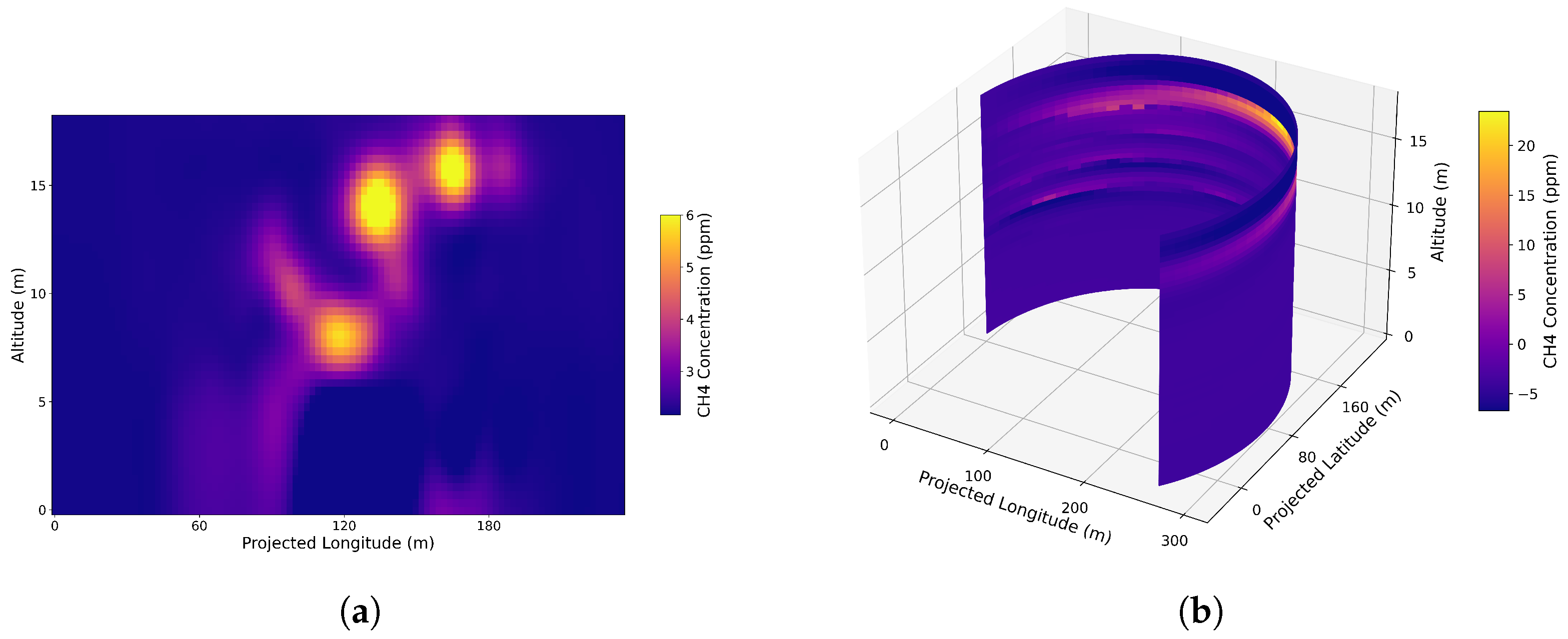
Figure 4 contrasts the curtain and arc heat maps, illustrating the spatial distribution of concentration measurements.
3.2. Comparison of Concentration Ratio Estimation Methods
The TFR method is a widely used approach for estimating CH4 emission rates using co-emitted or colocated tracer gases. This method relies on two critical assumptions: (1) the tracer gas must be released in close proximity to the emission source, and (2) concentration measurements of both the target and tracer gases must be collected at a downwind location where the plumes are fully co-dispersed. Satisfying the second condition typically requires sampling at considerable downwind distances, on the order of hundreds of meters, where the plumes have had sufficient time to merge.
When both of these conditions are reasonably satisfied, the slope method is traditionally used as the preferred concentration ratio estimation technique due to its simplicity and effectiveness. However, in many real-world applications, particularly for near-field measurements with sUAS, meeting both conditions is often infeasible due to logistical, regulatory, or spatial constraints. As such, this study investigates how alternative estimation approaches perform under scenarios where one or both TFR assumptions are violated.
To evaluate the robustness of different concentration ratio estimation techniques under these limitations, two experimental scenarios were designed:
Partial condition met: Condition 1 was satisfied—i.e., tracer and CH4 were co-emitted—but condition 2 was intentionally violated by collecting concentration measurements at relatively short downwind distances (tens of meters), rather than at the traditional hundreds of meters.
No conditions met: Neither condition was satisfied. Tracer and target gas sources were spatially separated, and concentration measurements were taken at near-field distances using sUAS to assess the impact of the estimation technique (slope, cumulative sum, integrated area, and peak value).
The performance of each concentration ratio method was assessed using both the relative error and the absolute uncertainty of the estimated CH4 emission rate. This evaluation provides insight into which approaches are most reliable when TFR assumptions are not feasible and helps inform optimal method selection for practical deployment in sUAS-based monitoring systems.
Results and Comparative Evaluation
In the whole gas release experiment, C2H6 was used as the tracer gas. Among the tested concentration ratio estimation methods, the cumulative sum approach yielded the lowest relative error of 3.31%, while the slope method provided the lowest absolute uncertainty at . This result suggests that both methods are viable under conditions where the tracer is co-emitted with the target gas and plume overlap is reasonably achieved.
In the mobile transect experiment, CH4 and N2O were co-emitted, and sampling was conducted using a ground-based mobile configuration. The slope method demonstrated the lowest relative error of −13.88%, while the cumulative sum method achieved the lowest absolute uncertainty, recorded at . This indicates that even with traditional ground-based sampling, the cumulative sum method remains a strong candidate when assessing emission rates at moderate downwind distances.
For the controlled release scenario involving spatially separated CH
4 and N
2O sources, the concentration ratio method performance varied depending on the sUAS flight pattern employed. In the curtain sampling configuration as summarized in
Table 3, the slope method produced both the lowest relative error (−38.22%) and the lowest absolute uncertainty
, highlighting its effectiveness under structured vertical flight sampling when conditions are moderately aligned with traditional TFR assumptions.
In contrast, the arc sampling method for the same spatially separated release showed different trends. As summarized in
Table 3, the peak value method yielded the lowest relative error at 8.8%, while the cumulative sum method resulted in the lowest absolute uncertainty at
. This shift underscores the sensitivity of each method to plume shape, overlap, and sampling strategy.
Two additional arc sampling experiments were conducted to assess the effect of vertical coverage. The first flight pattern covered an altitude range of 9–12 m. In this case, the peak value method again gave the lowest relative error (8.8%), and the cumulative sum method achieved the lowest absolute uncertainty . The second pattern extended the vertical coverage from 9 to 20 m. Here, the peak value method showed marked improvement in relative error, reducing it to 0.38%, while the cumulative sum method greatly lowered the absolute uncertainty to just .
These results collectively demonstrate that when full plume co-dispersion cannot be guaranteed, either due to downwind limitations or spatially separated releases, alternative methods such as the peak value and cumulative sum approaches offer more robust performance than the slope method. Moreover, as shown in
Table 4, increasing vertical coverage significantly improves estimation accuracy, reinforcing the advantage of sUAS sampling in real-world applications. Notably, for the slope method, plume segments were only included in the analysis if the correlation coefficient (
) exceeded 60%, ensuring the integrity of the linear regression.
In an alternative approach to evaluating tracer-based emission estimates, data from multiple individual plumes were concatenated and treated as a single composite dataset per flight pattern. This method was applied exclusively to sUAS-based experiments under both curtain and arc sampling configurations. Instead of analyzing each plume separately, this approach assumes the aggregated transects collectively represent a single, more robust measurement of the downwind signal. The curtain flight pattern produced notably lower relative errors and uncertainties for most estimation methods when compared to the arc. The slope method yielded a relative error of
with an uncertainty of
, while the cumulative sum and integrated area methods produced identical relative errors of
and uncertainties of
. The peak value method, while delivering the lowest relative error
, exhibited the highest uncertainty at
. For the arc configuration, the cumulative sum and integrated area again yielded consistent results (relative error:
; uncertainty:
), but the slope method was more biased (
) and uncertainty (
). Interestingly, the peak value method provided the best relative accuracy among arc estimates (
), but with the highest associated uncertainty (
), consistent with its volatility across trials. The effect of increased vertical sampling range was evident in the arc flights. Extending the flight ceiling from 12 m to 20 m significantly improved the slope method’s performance, reducing the relative error from
to
, and the uncertainty from 66.71 to
. The peak method also experienced a decrease in uncertainty (from 78 to
), albeit with a slightly worsened relative error (
). The cumulative sum and integrated area methods showed only slight changes in bias but benefited substantially in uncertainty, which dropped from
to just
. These results suggest that enhanced vertical coverage allows for better resolution of the plume’s spatial distribution, stabilizing the estimation metrics, especially for integration-based methods. These results are further illustrated in
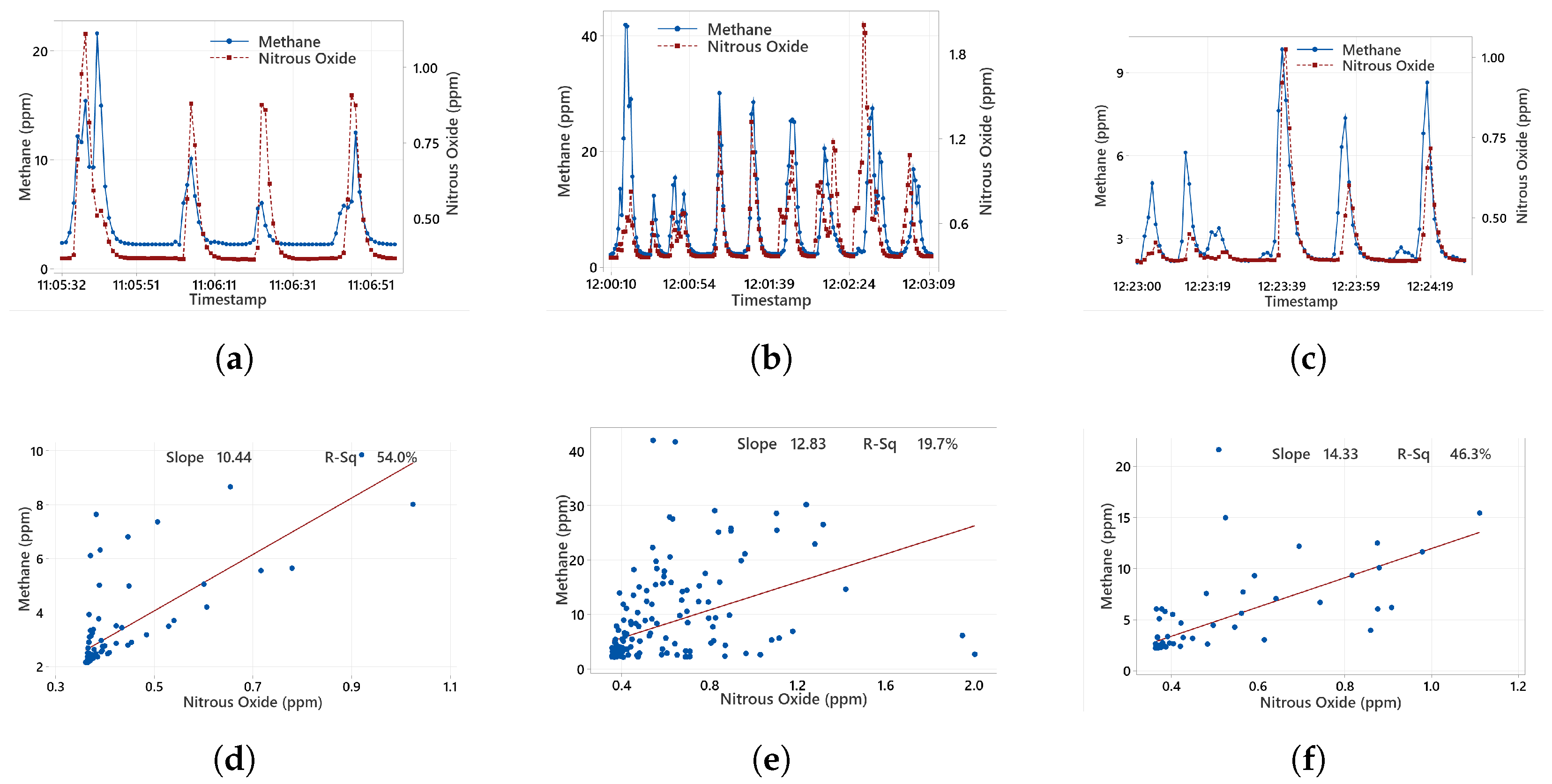
Figure 5, which shows time series data (
Figure 5a–c) for CH
4 and tracer concentrations across the curtain and arc flight patterns, as well as the corresponding regression fits (
Figure 5d–f). The curtain configuration, sampled at greater distances downwind, produced a more linear CH
4–tracer relationship (
Figure 5d), as indicated by a higher
value. In contrast, the arc pattern at 9–20 m altitude (
Figure 5e) exhibited weaker correlation, likely due to limited plume co-dispersion at the downwind sampling location, while the arc flight at 9–12 m (
Figure 5f) demonstrated improved linearity but resulted in higher uncertainty.
4. Discussion
This study demonstrates the effectiveness of using optimized sUAS-based methodologies to quantify CH4 emissions from natural gas facilities with high precision. By evaluating multiple flight configurations and ratio estimation methods across different tracer release scenarios, we identified operational tradeoffs and conditions that influence measurement accuracy. The arc flight pattern consistently outperformed the curtain approach, capturing the full lateral and vertical extent of the plume and enabling more robust integration of tracer and CH4 signals.
The accuracy of concentration ratio methods depended strongly on whether the two foundational TFR assumptions—co-located tracer release and full co-dispersion at the measurement location—were satisfied. Under ideal conditions, the slope method provided the lowest absolute uncertainty; however, in near-field scenarios or when plumes were not co-dispersed, cumulative sum and peak value approaches often yielded better relative accuracy. These results suggest that while the slope method remains a standard in field quantification, alternative methods are necessary when practical constraints prevent optimal sampling.
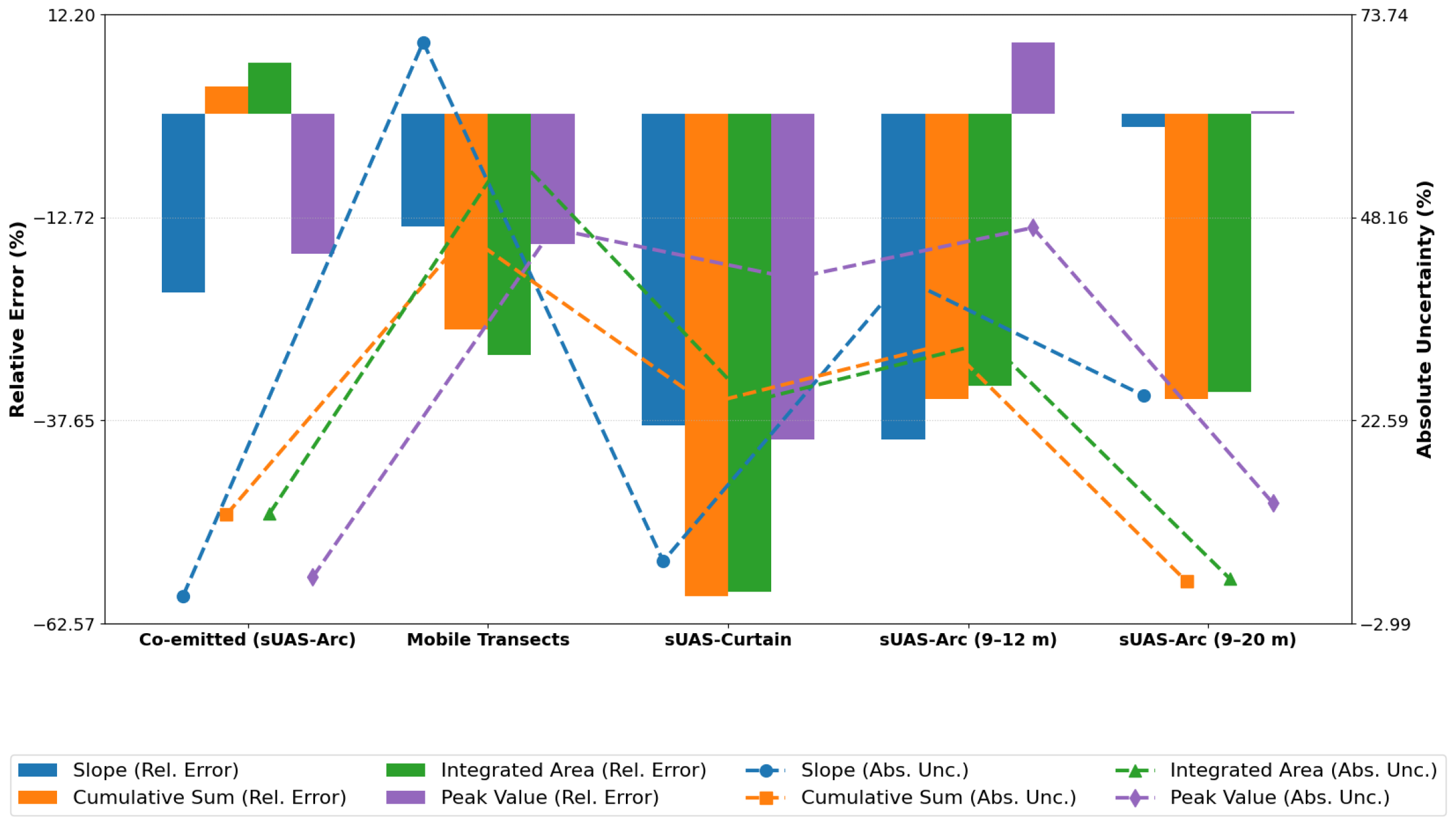
Figure 6 illustrates the variability in both relative error and absolute uncertainty across different measurement strategies. Notably, sUAS-based methods show a wide range of performance, highlighting the importance of method selection and operational parameters in achieving accurate emission estimates.
When comparing the composite approach to the original method of averaging across multiple plume-based estimates, several trends emerge. First, the bootstrapped composite method generally yields tighter uncertainty bounds, especially for integration-based estimators (cumulative sum and area), likely due to increased statistical power from the larger sample size. Second, the relative errors from the composite method tend to be more negative, particularly for the slope estimator, indicating a possible aggregation bias when combining plumes of varying shapes or magnitudes. However, for methods like peak value, the composite approach sometimes produces misleadingly low relative errors alongside inflated uncertainties, pointing to the sensitivity of this metric to noise and signal outliers. In contrast, the multiple-plume averaging approach tends to deliver more stable relative error metrics at the expense of slightly higher uncertainty due to variability between plume samples.
Ultimately, the composite method provides a compelling alternative when the assumption of a spatially and temporally coherent plume field is met. It offers enhanced uncertainty quantification through bootstrapping and highlights how flight geometry and vertical coverage influence estimator performance. These findings reinforce the importance of aligning flight strategy with the plume’s structure and the estimator’s mathematical assumptions.
Limitations and Future Work
Despite these promising results, several limitations warrant further attention. First, the temporal variability of emissions was not fully captured in short-duration flights. Incorporating longer-term monitoring campaigns will help assess diurnal and operational variability in emissions. Additionally, expanding the tracer framework to include isotopic signatures or co-emitted hydrocarbons could improve source attribution capabilities. Finally, future deployments should integrate automated flight planning based on real-time meteorological inputs to further reduce operator-induced uncertainty.
5. Conclusions
This study demonstrates a refined sUAS-based methodology for quantifying CH4 emissions from point source releases using the TFR technique. By combining optimized sampling strategies with controlled tracer deployment, we identified key drivers of uncertainty and bias in emission rate estimation.
In addition to traditional plume-by-plume analyses, we introduced a composite approach in which multiple transects collected during a single flight were aggregated and treated as a unified dataset. This method allowed for a more statistically robust evaluation of emission estimates by leveraging bootstrapping to quantify uncertainties across random subsets of the full data. The results showed that this composite strategy offers complementary insights to conventional averaging methods. In particular, integration-based estimators (e.g., cumulative sum and integrated area) benefited from tighter uncertainty bounds when applied to the aggregated data, while peak-based estimates continued to exhibit greater variability due to their sensitivity to transient spikes and outliers.
The arc flight pattern emerged as particularly effective for capturing the plume’s full spatial structure, especially when the vertical sampling range was extended from 9–12 m to 9–20 m. This expanded vertical coverage significantly reduced both relative errors and absolute uncertainties, underscoring the importance of altitude design in enhancing the accuracy of emission quantification. The curtain flight pattern, sampled at farther downwind distances, yielded higher values in regression fits and consistently performed well with slope-based estimators—suggesting improved alignment with Gaussian plume assumptions at greater distances.
Ethane, as a co-emitted tracer, was used to establish benchmark conditions and evaluate methodological tradeoffs. These benchmarks supported subsequent experiments using N2O, which showed improved ratio fidelity when tracer and CH4 plumes were closely aligned in space and time. Overall, our findings underscore the value of tailoring flight geometry, tracer selection, and estimation methodology to specific release conditions. The bootstrapped composite approach introduced here offers an additional layer of robustness by integrating uncertainty quantification directly into the estimation workflow. This makes it especially valuable for low-signal or noisy datasets where conventional plume-by-plume methods may struggle.
Looking ahead, future work will focus on the following:
Together, these advances aim to improve regulatory monitoring, bolster emissions reporting, and enable more effective CH4 mitigation strategies in the oil and gas sector.


 ,
, 
