SCADA-Based Comparative Assessment of Power Curve Modeling Methods for a Low-Power Vertical-Axis Wind Turbine

Abstract

Accurate modeling of wind turbine power curves is essential for performance assessment, energy forecasting, condition monitoring, and operational optimization in wind energy systems. This study presents a SCADA-based comparative assessment of established power curve modeling approaches through a single-site case study conducted on a low-power Vertical Axis Wind Turbine (VAWT) operating under real environmental conditions at the University of the Isthmus, located in the Isthmus of Tehuantepec, Oaxaca, Mexico. The evaluated methods included the maximum power curve, an aerodynamic model based on Blade Element Momentum Theory (BEMT), parametric approaches using polynomial and logistic regressions, and non-parametric data-driven methods based on Random Forest (RF), Gaussian Process Regression (GPR), and Kernel Density Estimation (KDE). One year of SCADA data, including wind speed and generated power measurements, was analyzed, while model performance was assessed using RMSE, MAE, and R² metrics. The results showed that the machine learning approaches achieved the lowest prediction errors among the evaluated models, with RF providing the best overall performance (RMSE = 7.4%, MAE = 4.8%, R² = 0.9814), followed by GPR and KDE under the investigated operating conditions. Additionally, Weibull analysis yielded parameters of k = 1.887 and c = 7.875 m/s, while the largest prediction errors were observed within the partial-load operating region (approximately 4–10 m/s) and as the turbine approached the rated operating condition (approximately 10–12 m/s). These findings indicate that, for the investigated low-power VAWT operating at the experimental site, non-parametric approaches provided the most accurate representation of the power curve among the evaluated models, highlighting the potential of SCADA-based data-driven techniques for comparative model assessment under similar operating conditions.

1. Introduction

The current population growth has led to an increasing demand for energy resources, which are often supplied through the use of fossil fuels such as oil, natural gas, and coal [1]. This energy model, besides being finite, generates significant environmental impacts and contributes substantially to climate change. In response to this challenge, renewable energy sources have gained a key role in the transition toward more sustainable, secure, and efficient power systems [2]. 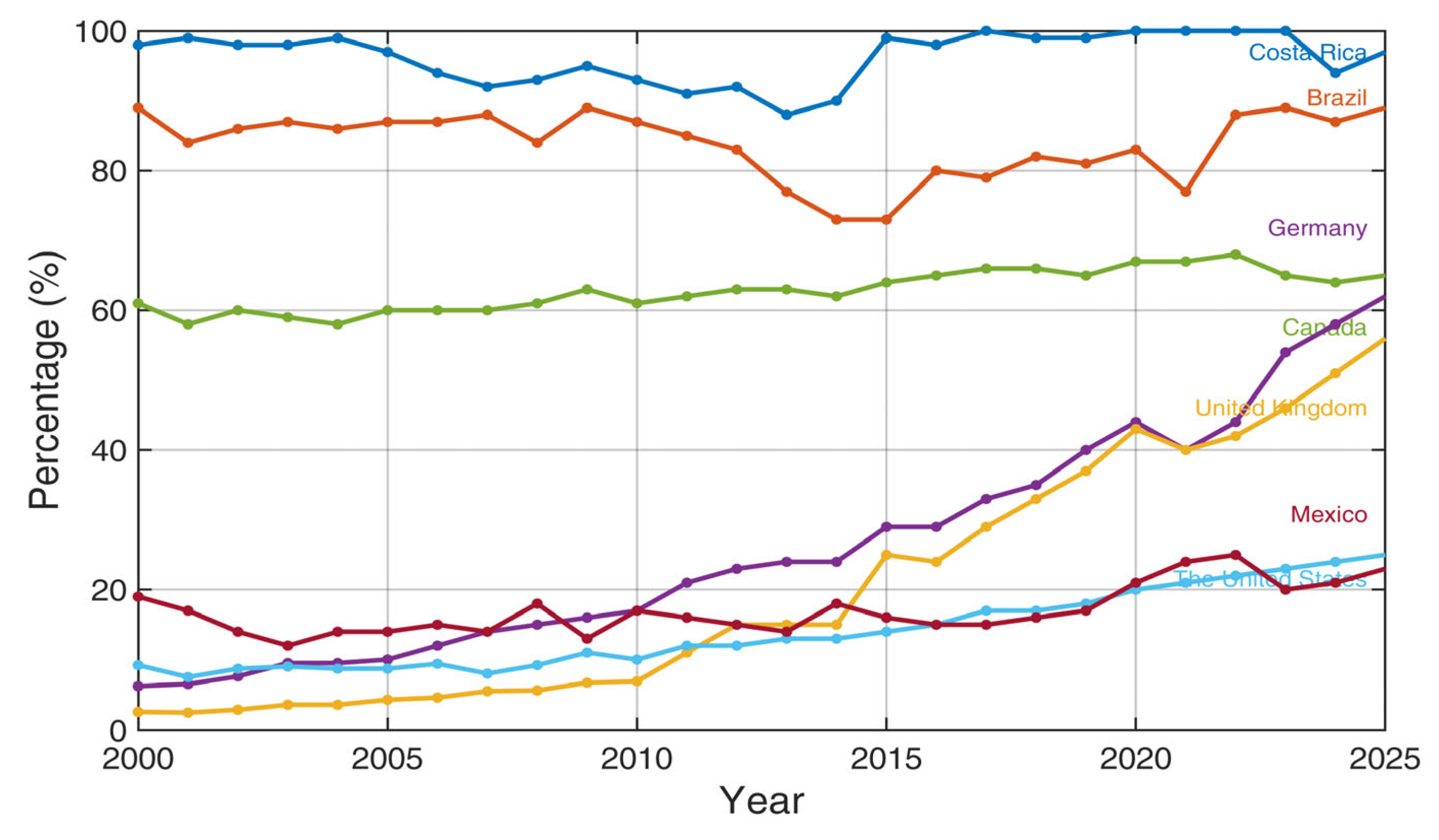Figure 1 illustrates the evolution of the share of renewable energy in global electricity generation during the period 2000–2025. At the global level, an increasing trend can be observed, particularly since 2010, reaching values above 30% in recent years, mainly driven by the expansion of wind and solar energy.

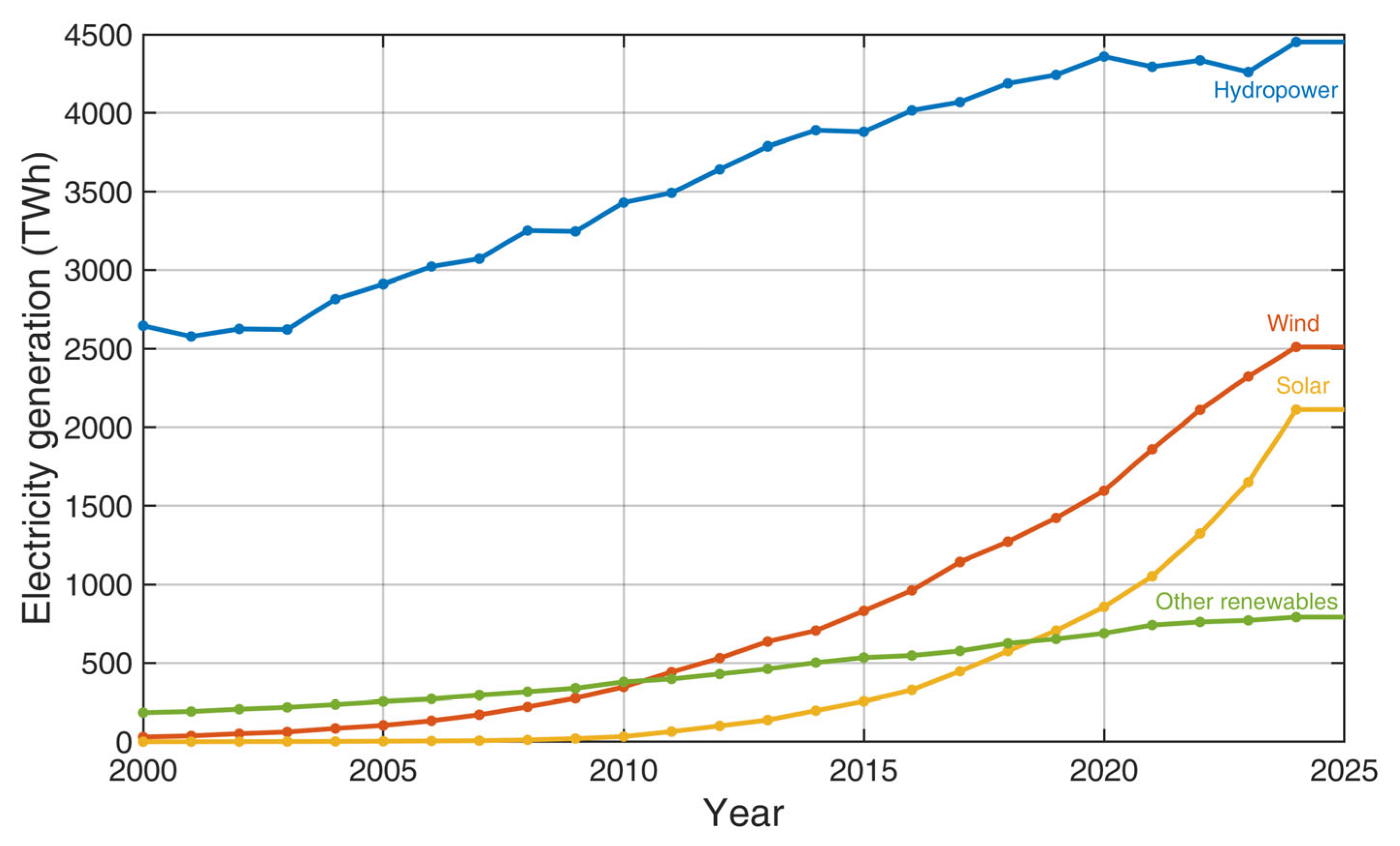
Figure 2 illustrates the evolution of global renewable electricity generation by technology between 2000 and 2025. While hydropower has remained the dominant renewable source, wind and solar energy have experienced the fastest growth over the last decade. In particular, wind energy has become a key component of the global energy transition due to its increasing installed capacity, technological maturity, and contribution to reducing greenhouse gas emissions [4,5,6].

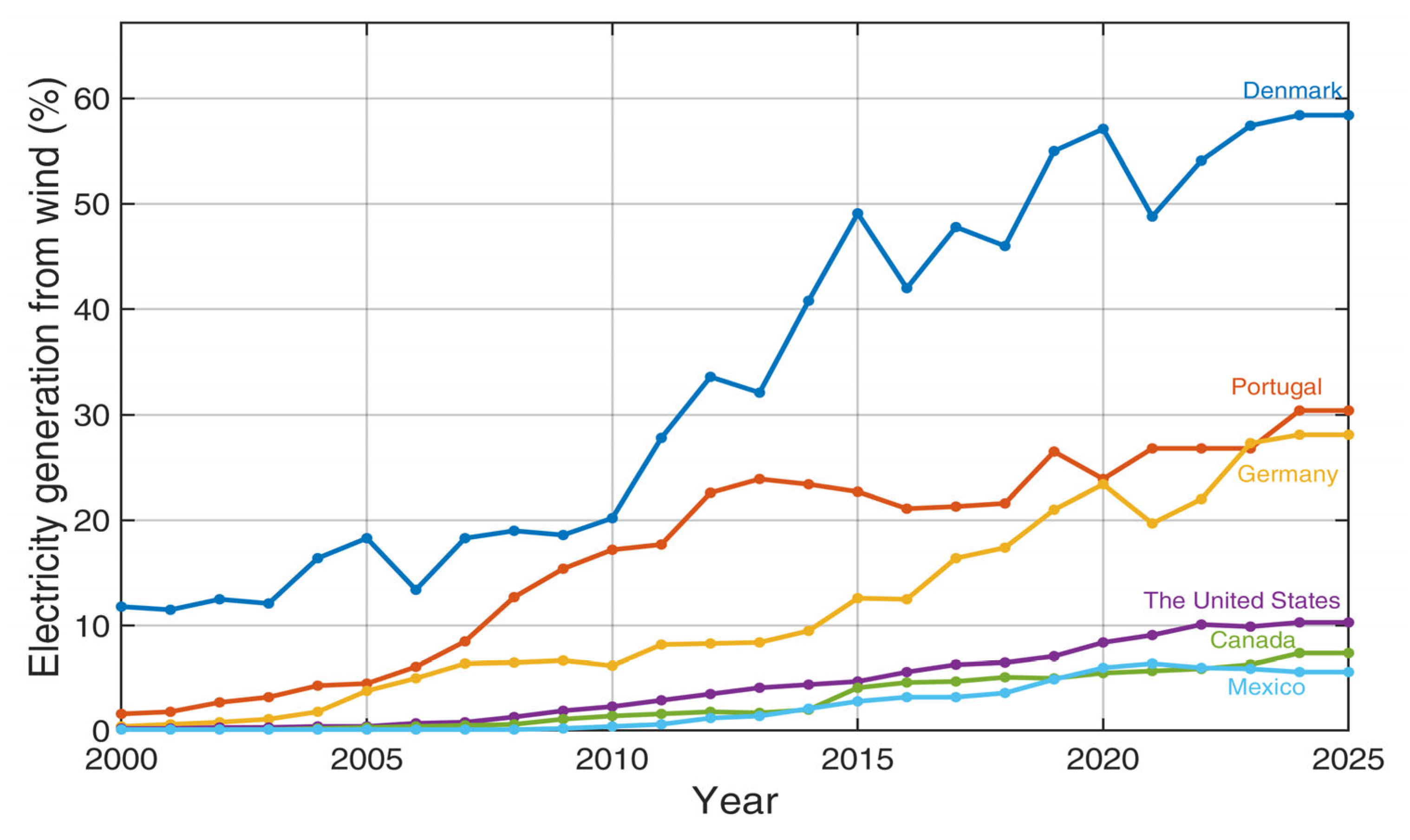
Figure 3 compares the evolution of wind power penetration in representative countries between 2000 and 2025. The results illustrate the sustained global expansion of wind energy, with countries such as Denmark, Portugal, and Germany achieving high levels of electricity generation from wind resources, while Mexico has shown continuous growth over the last decade. These trends highlight the increasing relevance of wind energy worldwide and the need for accurate performance assessment methods capable of supporting wind turbine operation under diverse environmental conditions.

Wind power forecasting is particularly challenging because it depends not only on wind speed but also on several additional factors. Turbulence phenomena can significantly alter the instantaneous power generated by a wind turbine, thereby complicating the development of stable predictive models [7,8]. Furthermore, variations in wind speed at different heights significantly affect turbine operation and, consequently, forecasting accuracy [9,10].

In this context, the accurate evaluation of wind turbine performance is essential to ensure the efficiency of wind power generation systems. Traditionally, energy generation forecasting for wind turbines has been based on the corresponding power curve [11]. However, previous studies have shown that this simplified approach may lead to forecasting errors ranging from 5% to 10% [12]. Within the rapidly expanding wind energy sector, wind turbine power curves play a crucial role in assessing both operational status and system performance [13,14]. The power curve represents the performance characteristics of a wind turbine and serves as an important indicator for evaluating its operational condition [14]. Moreover, it is widely used for operational monitoring, fault diagnosis, energy production estimation, and performance analysis under real operating conditions.

Therefore, selecting an appropriate modeling approach is critical to obtaining reliable evaluations and supporting decision-making processes.

Currently, the development of wind turbine power curves is mainly based on the standards established by the International Electrotechnical Commission (IEC 61400-12-1) [15,16]. However, under real operation and maintenance conditions in wind farms, factors such as turbine installation site, altitude, meteorological conditions, and environmental characteristics may significantly affect the accuracy of the power curve. Overestimation may negatively impact the service life of wind turbines, whereas underestimation can substantially affect power generation performance [14]. In vertical-axis wind turbines (VAWTs), power curve estimation presents additional challenges due to the pulsating nature of rotor motion, the dynamic effects of the incoming flow, and their sensitivity to turbulence. Furthermore, variations in wind speed at different heights also significantly influence turbine operation.

The wind turbine power curve describes the relationship between wind speed and generated electrical power and constitutes the primary indicator for evaluating turbine performance under operating conditions. Although manufacturer power curves are obtained under standardized test conditions, real operating environments are affected by turbulence, wind shear, air density, wind direction, and site-specific atmospheric conditions, leading to deviations from the nominal behavior [17,18,19,20,21,22,23]. Consequently, numerous statistical, analytical, and data-driven approaches have been proposed to improve power curve estimation under real operating conditions [23,24,25,26].

Despite the rapid development of wind energy, accurately representing the relationship between wind speed and power output under real operating conditions remains a significant challenge. The variability introduced by turbulence, atmospheric conditions, and site-specific effects limits the applicability of standardized power curves and motivates the development of more robust modeling approaches. Consequently, identifying the most suitable method for power curve estimation under realistic operating conditions has become an important research topic.

Traditionally, power curve modeling has been based on standardized approaches, with the method proposed in the IEC 61400-12-1 standard [16] being one of the most widely adopted in the wind energy industry. This method is based on grouping wind data into discrete intervals (binning) and calculating average power values for each interval. Although this approach provides a common framework for comparing wind turbine performance, its accuracy may be limited by data dispersion and the influence of variable atmospheric conditions.

In response to these limitations, several alternative methods have been developed for power curve modeling, which can generally be classified into statistical methods, analytical methods, and data-driven approaches. Statistical methods include polynomial regressions, sigmoid functions, logistic functions, and probability density-based models. In contrast, analytical methods are typically based on aerodynamic principles and physical models of wind turbine operation. Finally, data-driven approaches, such as artificial neural networks, support vector machines, and other machine learning algorithms, have gained increasing attention due to their ability to capture complex nonlinear relationships in real operational data.

Despite the wide variety of available methods, there is still no universal consensus regarding which approach provides the highest accuracy under different operating conditions. The accuracy of power curve models depends largely on factors such as the quality and quantity of available data, installation environment, model complexity, and the ability to generalize under unseen operating conditions [27,28]. Therefore, comparative evaluations are essential to analyze the performance of different power curve modeling approaches, identify their advantages and limitations, and establish objective criteria for their selection using real wind data.

This work presents a comparative evaluation of the main power curve modeling approaches applied to a vertical-axis wind turbine (VAWT) using real site data. The study considers the manufacturer’s power curve, aerodynamic models based on Blade Element Momentum Theory (BEMT), parametric models, machine learning-based non-parametric approaches, and statistical methods based on Kernel Density Estimation (KDE).

Although numerous studies have compared parametric, non-parametric, and machine learning-based power curve models, most of these investigations have focused on horizontal-axis wind turbines (HAWTs) or utility-scale wind farms operating under relatively stable wind conditions. In contrast, limited attention has been given to small-scale vertical-axis wind turbines (VAWTs) operating under highly turbulent wind regimes. The Isthmus of Tehuantepec, Mexico, is recognized as one of the world’s most energetic wind corridors, characterized by strong seasonal winds, high turbulence intensity, and frequent gust events. These challenging aerodynamic conditions may significantly influence the predictive performance of different power curve modeling approaches. Therefore, a comprehensive comparative assessment of conventional, statistical, and machine learning-based power curve models for small-scale VAWTs under these operating conditions remains insufficiently explored in the literature.

To address this research gap, this study comparatively evaluates the performance, predictive accuracy, and robustness of conventional, parametric, statistical, and machine learning-based power curve modeling approaches for a small-scale vertical-axis wind turbine operating under the highly turbulent wind conditions of the Isthmus of Tehuantepec, Mexico. By assessing these methods using one year of real operational data, this study aims to identify the most suitable modeling approach for VAWT performance evaluation while providing new insights into the behavior of different modeling techniques under complex atmospheric conditions. The findings contribute to filling the existing research gap regarding power curve modeling for small-scale VAWTs and provide a useful reference for future monitoring, performance assessment, and optimization of wind energy systems.

This work presents a SCADA-based comparative case study conducted on a low-power vertical-axis wind turbine installed at the University of the Isthmus, Tehuantepec campus. The objective is to evaluate and compare the predictive capability of established analytical, parametric, statistical, and machine learning power curve models under the specific operating conditions of the experimental site. Therefore, the findings and conclusions of this study are limited to the investigated turbine and the corresponding measurement conditions.

2. Materials and Methods

This study evaluates seven representative power curve modeling approaches using the same experimental SCADA dataset acquired from a small-scale vertical-axis wind turbine (VAWT). The evaluated approaches include the manufacturer’s reference power curve, the Blade Element Momentum Theory (BEMT) model, polynomial regression, logistic regression, Random Forest (RF), Gaussian Process Regression (GPR), and Kernel Density Estimation (KDE). All methods were implemented under identical preprocessing, training, validation, and evaluation conditions to ensure a fair comparison of their predictive performance. The following subsections briefly describe the implementation of each modeling approach adopted in this study.

In this study, Blade Element Momentum Theory (BEMT) was implemented as the physics-based reference model for power curve estimation. The model was applied using the aerodynamic characteristics of the studied vertical-axis wind turbine (VAWT), considering its geometric parameters and operating conditions. Although BEMT provides a physically interpretable representation of wind turbine performance, its application to VAWTs remains challenging because of dynamic stall effects, large variations in the angle of attack during rotor rotation, and complex wake interactions [16,25].

Polynomial and logistic regression models were implemented as representative parametric approaches. Both models were fitted using the experimental wind speed and power measurements obtained from the SCADA database. These methods provide computationally efficient approximations of the power curve and serve as reference parametric models for comparison with the machine learning approaches evaluated in this study [29].

Random Forest (RF) and Gaussian Process Regression (GPR) were implemented as non-parametric machine learning models. Both algorithms were trained using the same experimental dataset and identical preprocessing conditions to evaluate their capability to model the nonlinear relationship between wind speed and generated power. Their performance was subsequently compared with that of the analytical and parametric approaches using the same evaluation metrics [30,31].

Kernel Density Estimation (KDE) was implemented as a probabilistic statistical approach to estimate the conditional distribution of wind turbine power output. This method was evaluated using the same SCADA dataset and preprocessing procedure adopted for all other models, allowing a direct comparison under identical experimental conditions.

2.1. Manufacture’s Power Curve

As a starting point for the comparative evaluation of the different modeling approaches, the power curve of the manufacturer of the SX-2000W vertical axis commercial wind turbine, from a commercial supplier in China, was considered as a baseline reference for the comparison of model. This curve represents the nominal performance of the turbine under standardized testing conditions and is widely used as a reference in energy performance studies and model validation.

The power curves provided in turbine catalogs are based on a theoretical model consistent with the IEC 61400-12-1 standard [16], which can be expressed as follows:

$$\mathit{P}={\displaystyle \frac{1}{2}}\rho A{v}^3{C}_p$$

(1)

where ρ is the air density $(\mathrm{k}\mathrm{g}/{\mathrm{m}}^3$); A is the rotor swept area (${\mathrm{m}}^2$); v is the wind speed (m/s); and C_p is the power coefficient (dimensionless).

In the particular case of vertical-axis wind turbines (VAWTs), the swept area is defined as the projected area of the rotor and can be calculated as follows:

A = DH = 2RH

(2)

where D is the rotor diameter (m), R is the rotor radius (m), and H is the rotor height (m). This formulation differs from horizontal-axis wind turbines (HAWTs), in which the swept area is circular. Furthermore, the mechanical power can be related to the aerodynamic torque Q and the angular velocity (N m) as follows:

P = wQ

(3)

which is particularly useful for the dynamic characterization of vertical-axis rotors.

In theory, the amount of power generated by a wind turbine is modeled as a function of the rotor swept area, air density, and the kinetic energy flux incident on the turbine rotor. Turbine designers optimize design parameters, such as blade geometry, rotor diameter, and generator power rating, based on the annual wind forecast at the installation site and subsequently provide the power curve of the designed turbine [12].

In practical terms, the manufacturer’s power curve is typically expressed as a deterministic function of wind speed, defined by distinct operating regions: (i) the cut-in region, where the generated power is zero below the cut-in wind speed; (ii) the power growth region, where power increases nonlinearly with wind speed; (iii) the rated power region, where the generated power remains approximately constant; and (iv) the cut-out region, where turbine operation is stopped for safety reasons.

However, the manufacturer’s power curve is obtained under standardized conditions that differ significantly from real operating environments, particularly in the case of vertical-axis wind turbines (VAWTs). Factors such as wind variability, turbulence, unsteady aerodynamic losses, and site-specific conditions may lead to significant discrepancies between the nominal power curve and the actual power produced in field operation [32].

In this study, the manufacturer’s power curve is used exclusively as a theoretical baseline reference against which the different power curve modeling approaches are compared. Its inclusion enables the evaluation of the degree of deviation between nominal performance and the actual behavior of the wind turbine, as well as the quantification of improvements achieved through advanced modeling approaches adapted to real operating conditions.

2.2. Aerodynamic Models Based on Blade Element Momentum Theory (BEMT)

The conventional BEMT model was included to provide a physics-based analytical baseline for comparison rather than an optimized aerodynamic representation of VAWT performance. Accordingly, its purpose in this study is not to compete with data-driven models, but to provide a well-established analytical reference for evaluating the predictive capabilities of different power curve modeling approaches under identical operating conditions.

In the present study, a simplified BEMT implementation was adopted to provide a consistent analytical benchmark for comparison with the parametric and machine learning approaches. The implemented model considers the rotor geometry (swept area), air density, maximum power coefficient, cut-in wind speed, and rated operating conditions to estimate the generated power. However, detailed blade-element discretization, airfoil-specific aerodynamic coefficients, dynamic stall modeling, rotational induction corrections, and other advanced aerodynamic effects were not incorporated, since the objective was to establish a common physics-based reference rather than to develop a high-fidelity aerodynamic model.

Aerodynamic modeling of vertical-axis wind turbines (VAWTs) using BEMT-based approaches has been widely addressed in the literature [33,34]. In these models, aerodynamic forces are calculated from the lift and drag coefficients, which depend on the instantaneous angle of attack and the relative flow velocity [33,35]. However, the periodic variation in the angle of attack and unsteady aerodynamic effects introduce limitations in model accuracy, particularly under turbulent wind conditions [36,37]. Despite these limitations, BEMT models continue to be used as a physics-based reference for power curve estimation in VAWTs. This method combines the principles of linear and angular momentum conservation with the local aerodynamic analysis of blade elements, enabling the estimation of the aerodynamic forces acting on the rotor and, consequently, the generated mechanical power.

From a theoretical perspective, BEMT divides each wind turbine blade into a set of differential elements distributed along its span. For each element, the aerodynamic forces are calculated from the lift and drag coefficients, which depend on the local angle of attack and the airfoil characteristics. The differential aerodynamic force acting on a blade element can be expressed as follows:

$$\mathit{dF} = {\displaystyle \frac{1}{2}}\rho v_{\mathit{rel}}^{2}c\left(C_L{e}_L + C_D{e}_D\right)\mathit{dr}$$

(4)

where ρ is the air density, $v_{rel}$ is the relative flow velocity over the blade element (m/s), c is the airfoil chord length (m), $C_L$ and $C_D$ are the lift and drag coefficients (dimensionless), respectively, $e_L$ and $e_D$ are the unit vectors associated with the lift and drag directions (dimensionless), and r is the radial coordinate of the blade element.

In vertical-axis wind turbines (VAWTs), the relative velocity v(rel) and the angle of attack vary periodically with the azimuthal position of the blade. The relative velocity can be expressed as a combination of the incoming wind speed v and the tangential velocity of the blade [33,38].

$$V_{\mathrm{rel}}=\sqrt{(v\mathrm{Cos}\theta {)}^2+(\mathit{wr}+v\mathrm{Sin}\theta {)}^2}$$

(5)

where is the azimuthal angle of the blade and w is the angular velocity of the rotor.

The instantaneous angle of attack α, a key parameter in the determination of aerodynamic coefficients, is calculated as follows:

$$\mathsf{\alpha } = \arctan \left({\displaystyle \frac{v \mathrm{Cos} \theta }{\mathit{wr}+\mathrm{v} \mathrm{Sin} \theta }}\right)- \beta$$

(6)

where β represents the blade pitch angle.

The aerodynamic forces calculated for each blade element are projected onto the tangential direction of the rotor to obtain the differential aerodynamic torque, expressed as follows:

$$\mathrm{d}Q=rd{F}_t$$

(7)

where ${\mathrm{dF}}_{\mathrm{t}}$, is the tangential component of the aerodynamic force (N). The total rotor torque is obtained by integrating the differential torque along the blade span and over the complete rotation cycle [18,38].

$$\mathrm{Q}={\int }_0^{2\mathsf{\pi }}{\int }_{{\mathrm{r}}_{\min }}^{{\mathrm{r}}_{\max }}\mathrm{d}Q \mathrm{d}r \mathrm{d}\theta$$

(8)

Finally, the power coefficient of the model is defined as follows:

$$C_p = {\displaystyle \frac{P}{\frac{1}{2}\rho A{v}^3}}$$

(9)

Although BEMT has been widely applied to horizontal-axis wind turbines, its application to vertical-axis wind turbines introduces additional challenges, including large variations in the effective angle of attack during each rotor revolution, pronounced dynamic stall effects, and complex wake interactions.

For this reason, the conventional BEMT model was not intended to represent the most advanced aerodynamic model for VAWTs. Instead, it was included as a physics-based baseline to provide a common analytical reference for comparing conventional analytical modeling with data-driven approaches under identical operating conditions. Consequently, the objective of this comparison is not to demonstrate the superiority of machine learning over BEMT, but rather to quantify the predictive capability of different modeling paradigms when applied to the same experimental dataset.

2.3. Parametric Power Curve

Parametric power curve models are based on approximating the relationship between wind speed and generated power using predefined mathematical functions characterized by a finite number of parameters. This approach has been widely used in wind turbine performance assessment studies due to its computational simplicity, interpretability, and ease of implementation [39,40,41].

From a physical perspective, the power generated by a wind turbine mainly depends on the cubic behavior of wind speed, as derived from

$$P(v) = {\displaystyle \frac{1}{2}}\rho C_p(v\left)\right(v^3)$$

(10)

where A corresponds to the rotor swept area. In vertical-axis wind turbines (VAWTs), this area is defined as A = 2RH, which introduces a linear geometric dependence on the rotor height. However, under real operating conditions, the power coefficient C_p exhibits saturation effects, losses, and smooth transitions between operating regions; therefore, the cubic relationship is modified. Parametric models aim to empirically approximate this nonlinear response.

In general, the parametric power curve can be expressed as follows:

P(v) = f(v;θ)

(11)

where v is the wind speed (m/s), P(v) is the estimated power output (W), and θ is the vector of model parameters.

Two main groups of parametric models are considered: polynomial models and sigmoid-type logistic models, which enable the representation of the gradual transition between the cut-in, partial-load operation, and rated operating regions of the wind turbine.

2.3.1. Polynomial Models

The polynomial model constitutes one of the simplest and most widely used approaches. In this model, power is expressed as a linear combination of wind speed powers and has been extensively applied in the literature for wind turbine power curve estimation. Its general form is defined as follows [39,40,41]:

$$P\left(v\right) = {\sum }_{i=0}^n{a}_i{v}^i$$

(12)

where a_i are the polynomial coefficients and n is the order of the model. Small values of n lead to smooth and stable models, whereas higher orders increase flexibility, although they may induce spurious oscillations and overfitting.

This model has been widely used to approximate empirical power curves due to its ability to fit measured data within a limited wind speed range [40]. However, higher-order polynomials may introduce non-physical oscillations and overfitting problems, particularly in regions with high data dispersion [41].

For this reason, low- and medium-order polynomials were evaluated in this study, and the optimal model was selected based on fitting accuracy and numerical stability.

2.3.2. Sigmoid-Type Logistic Models

Logistic functions provide a more realistic description of the characteristic S-shaped power curve, naturally capturing power saturation within the rated operating region of the wind turbine [42,43,44].

The four-parameter logistic function is expressed as follows:

$$P(v) = {\displaystyle \frac{P_{\mathit{max}}}{1 + \mathit{exp}[-k\left(v - V_o\right)]}}$$

(13)

where P_max is the maximum power output (W), k controls the transition slope, and ${\mathrm{v}}_{\mathrm{o}}$ represents the wind speed associated with the inflection point of the curve (m/s).

In some studies, a five-parameter formulation is employed to improve model flexibility [45].

$$P(v) = P_{\mathit{min}}{\displaystyle \frac{P_{\mathit{max}}-P_{\mathit{min}}}{1+\mathit{exp}[-k\left(v-V_o\right)]}}$$

(14)

This type of formulation has demonstrated good performance in modeling power curves derived from SCADA data and field measurements for both vertical-axis and horizontal-axis wind turbines [44,45].

To improve fitting flexibility, a generalized formulation is considered:

$$P\left(v\right) = P_r(1 + \mathit{exp}[-k\left(v-v_o\right)]{)}^{-m}$$

(15)

where m controls the asymmetry of the transition (dimensionless).

Logistic functions generally exhibit greater numerical stability than polynomial models and produce smoother curves, which are desirable characteristics for forecasting and control applications.

2.3.3. Parameter Estimation

The parameters of the polynomial and logistic models were estimated using the least-squares method by minimizing the sum of squared errors between the measured power values and the model-estimated values [39,40].

$$\mathit{min}{\displaystyle {\sum }_{j=1}^N}(P_{\mathit{med}}\left(\mathit{vj}\right)-P (\mathit{vj}; \theta ){)}^2$$

(16)

where N is the number of available observations (dimensionless) and ${\mathrm{P}}_{\mathrm{med}}$ represents the power measured in field operation (W).

2.4. Non-Parametric Machine Learning Models

To capture the complex nonlinear relationships and high statistical dispersion present in wind turbine field data, non-parametric machine learning models were employed. Unlike parametric approaches, these methods do not impose a predefined functional form for the power curve; instead, they directly infer the relationship between variables from the observed data. This characteristic makes them particularly suitable for real operating conditions, where turbulence, flow dynamic effects, and aerodynamic losses introduce behaviors that are difficult to represent using simple analytical functions [46,47].

In this study, two approaches widely used in the recent literature were implemented: Gaussian Process Regression (GPR) and Random Forest (RF).

In general, the modeling problem can be formulated as follows:

$$P=\mathit{f}\left(x\right)+\epsilon$$

(17)

where P is the generated power output (W), x represents the input variable vector, f is an unknown function to be estimated, and ε is a random noise term.

Non-parametric methods are particularly suitable when the relationship between wind speed and generated electrical power exhibits complex structures, multimodal behavior, or heterogeneous variability across different wind turbine operating regimes.

2.4.1. Gaussian Process Regression (GPR)

Gaussian Process Regression (GPR) constitutes a Bayesian probabilistic approach for estimating unknown functions. Within this framework, the latent function f(x) is assumed to follow a Gaussian process defined by a mean function m(x) and a covariance function k(x, x′) [46,47,48]

$$P_i=f \left(v_i\right)+{\epsilon }_i, {\epsilon }_i\sim N \left(0, {\sigma }_n^2\right)$$

(18)

and the latent function is assumed to be distributed as follows:

$$f\left(x\right)\sim \mathit{GP}\left(m\right(x\left)\right), k \left(x, x’\right)$$

(19)

A zero-mean function, m(x) = 0, is commonly adopted; therefore, the model behavior is entirely determined by the kernel function. Given a training dataset D = {(x_i, P_i)}_i=1^N, predictions for a new input point x follow a Gaussian distribution.

In practice, the Radial Basis Function (RBF) kernel is commonly employed:

$$k (x, x^{\prime }) ={ \sigma }_f^2\mathit{exp}(-{\displaystyle \frac{{\Vert x-x^{\prime }\Vert }^2}{2l^2}})$$

(20)

where ${\mathsf{\sigma }}_{\mathrm{f}}^2$ is the process variance and l is the length scale controlling the smoothness of the estimated function. The hyperparameters (${\mathsf{\sigma }}_{\mathrm{f}}, \mathrm{l}, {\mathsf{\sigma }}_{\mathrm{n}})$ are estimated by maximizing the marginal likelihood of the training data.

This probabilistic approach has proven to be particularly effective for modeling power curves with high operational variability and noise in real-world data, providing more robust estimations than traditional parametric methods [49].

2.4.2. Random Forest (RF)

The Random Forest (RF) algorithm is a non-parametric ensemble learning method that constructs multiple decision trees using randomly sampled subsets of the training data and subsequently averages their predictions to obtain a more stable and robust estimate. Formally, if ${\mathrm{T}}_{\mathrm{b}}(\mathrm{v})$ represents the prediction of tree b (W), the final prediction is given by:

$$\widehat{P}(v) = {\displaystyle \frac{1}{B}}{\sum }_{\mathrm{b}=1}^{\mathrm{B}}{T}_b\left(\mathrm{v}\right)$$

(21)

where B is the total number of trees in the model (dimensionless). Each tree is trained using a bootstrap sample of the training dataset and a random subset of variables at each node split, thereby reducing the correlation among trees and improving generalization performance.

Random Forest is particularly useful when strong nonlinearities, interactions among variables, and data noise are present, as commonly occurs in field measurements of wind turbines operating under real environmental conditions. Furthermore, this method is less susceptible to overfitting and is robust against outliers, which are typical challenges in SCADA datasets [50,51].

In this study, the Random Forest regression model was implemented using MATLAB’s R2021 b TreeBagger function. The model consisted of 300 regression trees generated through bootstrap aggregation. Since wind speed was the only predictor variable considered in this study, it was used at each node split during tree construction. A minimum leaf size of five observations was adopted as the stopping criterion to reduce overfitting while preserving the model’s generalization capability. The maximum tree depth was not explicitly constrained; instead, tree growth was automatically terminated according to the minimum leaf size criterion.

2.4.3. Kernel Density Estimation (KDE)

Kernel Density Estimation (KDE) is a non-parametric statistical method used to estimate the probability density function of a random variable from observed data without assuming a predefined parametric distribution [52,53,54]. In the context of power curve modeling, KDE enables the characterization of the conditional distribution of generated power as a function of wind speed, making it particularly suitable for datasets with high variability and noise, which are commonly observed in vertical-axis wind turbines operating under real-world conditions.

The conditional power density for a given wind speed v is estimated as follows:

$$\left(P\right|\mathrm{v}) = {\displaystyle \frac{1}{\mathit{Nh}}}{\sum }_{i=1}^{N}K \left({\displaystyle \frac{P-P_i}{h}}\right)$$

(22)

where N is the number of observations (dimensionless), h is the bandwidth parameter controlling the smoothness of the estimated density (W), and K is the kernel function (dimensionless).

In the proposed implementation, wind speed acts as the conditioning variable in the KDE framework. For each target wind speed, Gaussian kernel weights are assigned to the neighboring training observations according to their distance from the target value. The conditional probability density f(P∣v) is then estimated using these weighted observations, allowing the expected power output to be obtained as a smooth non-parametric function of wind speed.

A Gaussian kernel is commonly adopted:

$$K(u) = {\displaystyle \frac{1}{\sqrt{2\pi }}}\mathit{exp}(-{\displaystyle \frac{u^2}{2}})$$

(23)

The bandwidth h is a critical parameter that governs the trade-off between estimator bias and variance. In this study, the optimal bandwidth was selected using Silverman’s rule [54].

$$H = 1.06\widehat{\mathsf{\sigma }}{\mathit{N}}^{-1/5}$$

(24)

where $\widehat{\mathsf{\sigma }}$ is the standard deviation of the data. The expected power curve is then obtained as the conditional mean of the estimated density:

$$\widehat{P}\left(v\right) = \int P\widehat{f}\left(P\right|v) \mathrm{d}P$$

(25)

This approach provides a flexible and robust representation of the power curve, capturing multimodal behavior and asymmetric distributions that are difficult to represent using conventional parametric or deterministic methods.

2.5. Model Evaluation and Comparison Metrics

To objectively compare the performance of the different power curve modeling methods, including the BEMT-based aerodynamic approach, parametric models, non-parametric machine learning models, and the probabilistic quantile-based approach, a comprehensive set of statistical metrics was defined to evaluate both deterministic accuracy and the quality of probabilistic predictions. The adoption of multiple indicators is necessary due to the highly dispersed and heteroscedastic nature of field-measured power data, particularly in vertical-axis wind turbines, where variability induced by turbulence, local wake effects, and dynamic phenomena generates non-Gaussian errors [31,54].

Recent studies on power curve modeling based on SCADA data recommend combining metrics based on average error, global fitting performance, and probabilistic reliability to achieve a more robust evaluation of predictive performance [54,55,56].

Deterministic Metrics

Deterministic metrics are applied to models that provide point estimates, ${\widehat{\mathrm{P}}}_{\mathrm{i}}$, such as BEMT, polynomial models, logistic functions, and Random Forest.

The Root Mean Square Error (RMSE) is widely used in wind power modeling studies due to its sensitivity to large deviations and its ability to strongly penalize high-magnitude errors [30,57].

$$\mathit{RMSE} = \sqrt{{\displaystyle \frac{1}{N}}{\displaystyle {\sum }_{i=1}^N}(P_i-{\widehat{P}}_i{)}^2 }$$

(26)

where ${\mathrm{P}}_{\mathrm{i}}$ and ${\widehat{\mathrm{P}}}_{\mathrm{i}}$, correspond to the measured and estimated power values, respectively.

The Mean Absolute Error (MAE) provides a more robust measure against outliers and asymmetric error distributions, which are common characteristics in real wind turbine measurements [57].

$$\mathit{MAE} = {\displaystyle \frac{1}{N}}{\displaystyle {\sum }_{i=1}^N}\left|P_i-{\widehat{P}}_i\right|$$

(27)

The coefficient of determination (R²) evaluates the proportion of variance explained by the model and is frequently used to quantify the overall descriptive capability of the fitted curve [57].

$$R^{2 }=1 - {\displaystyle \frac{{\displaystyle {\sum }_{i=1}^N}{(P_i-{\widehat{P}}_i)}^2}{{\displaystyle {\sum }_{i=1}^N}{(P_i-P)}^2}}$$

(28)

where $\stackrel{\mathrm{-}}{\mathrm{P}}$ is the mean value of the observed data.

3. Data Description

3.1. Experimental Site

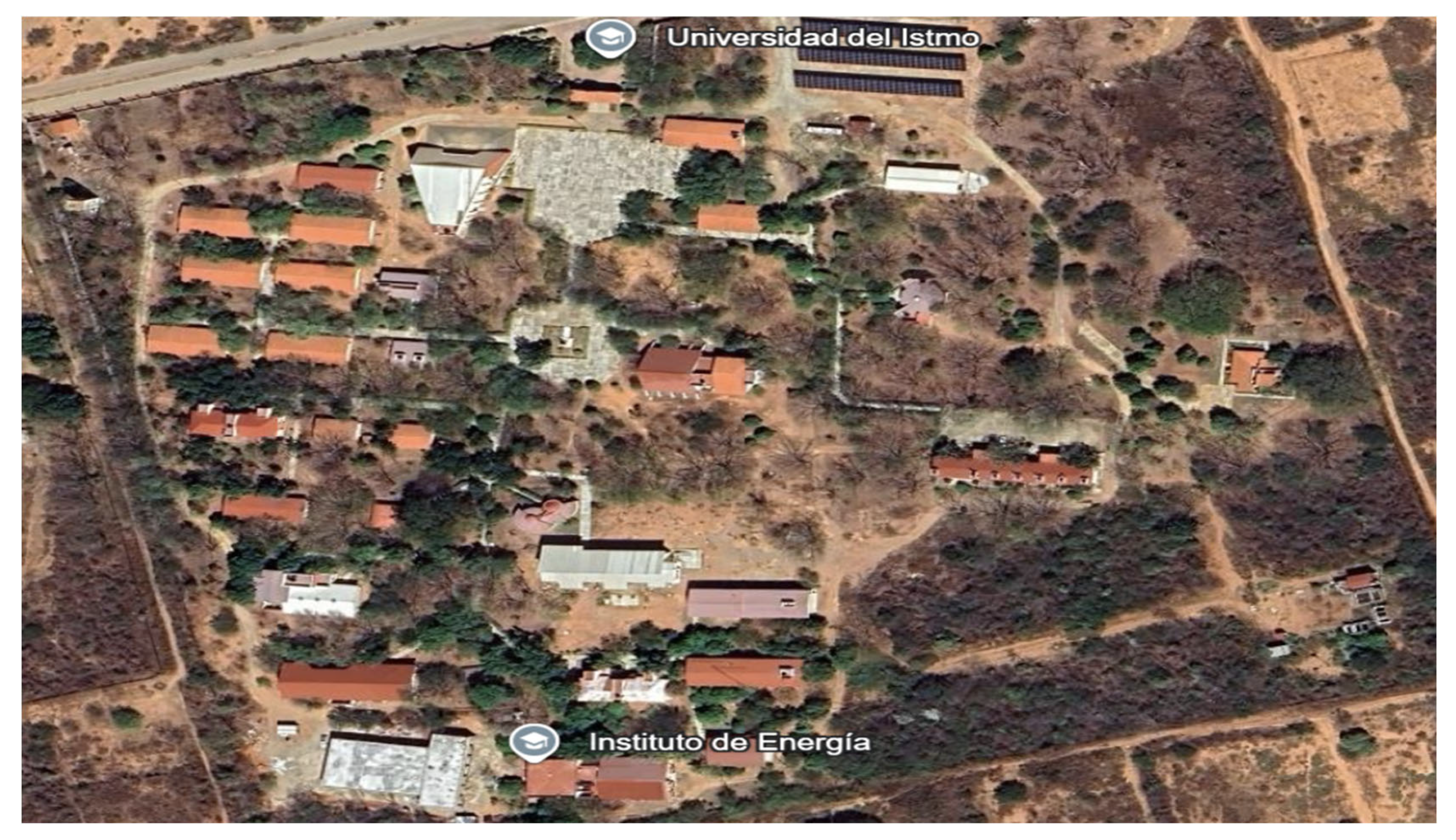
The experimental campaign was conducted at the University of the Isthmus (UNISTMO), Tehuantepec campus, Oaxaca, Mexico, located within the Isthmus of Tehuantepec, one of the world’s most important wind corridors. The site is characterized by persistent northerly winds, high wind resource availability, and atmospheric conditions representative of real operating environments for vertical-axis wind turbines.

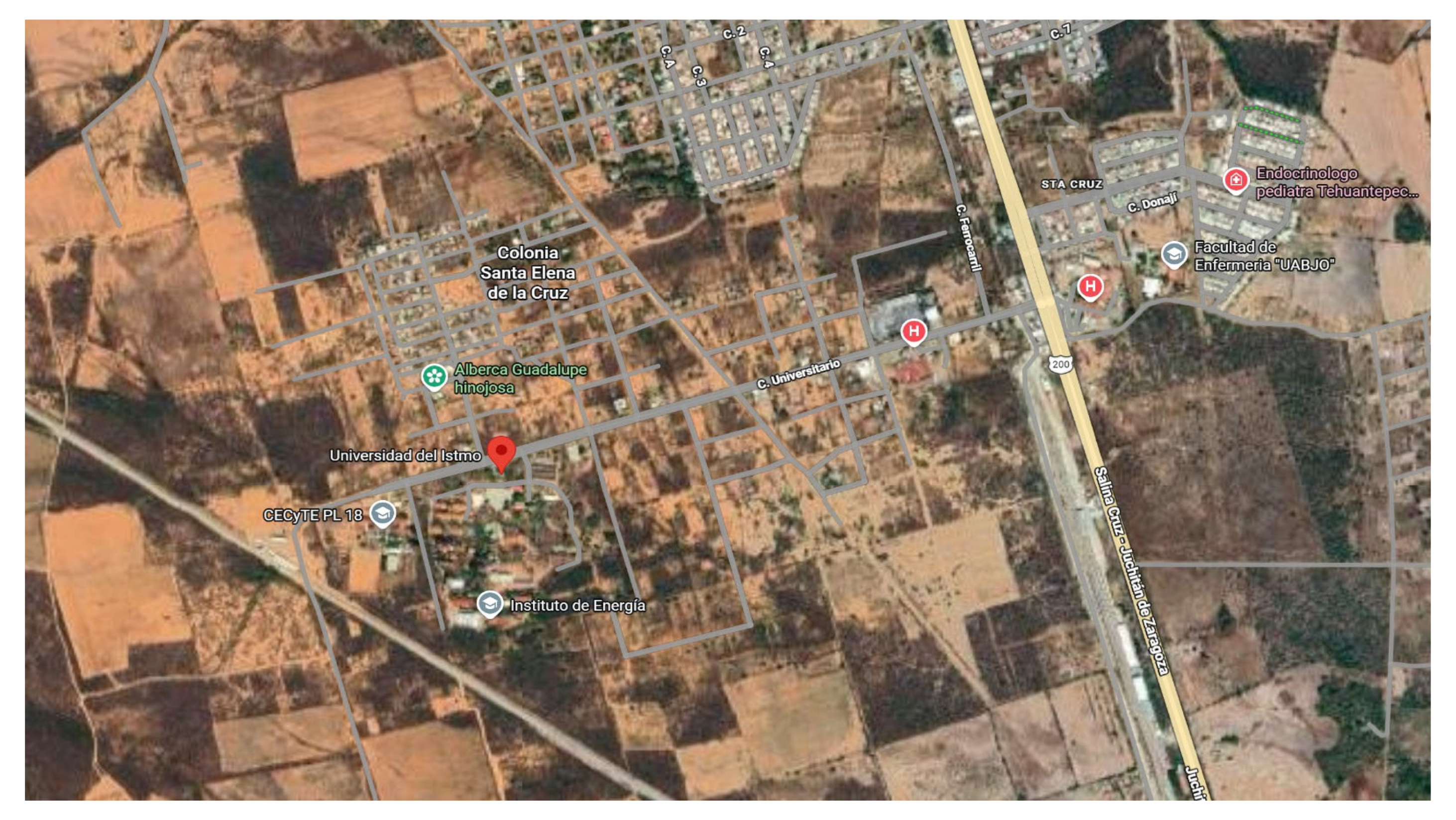
Figure 4 and Figure 5 illustrate the geographical location of the experimental site. The relatively flat terrain and the regional pressure gradients between the Gulf of Mexico and the Pacific Ocean promote strong and persistent wind conditions characteristic of the Tehuantepec wind phenomenon.

The experimental site exhibits variable wind speeds and turbulence levels representative of real operating conditions. These characteristics are particularly suitable for evaluating the aerodynamic performance and power curve modeling of vertical-axis wind turbines, whose aerodynamic response is highly sensitive to variations in wind direction and speed, as well as to unsteady phenomena of the incoming flow.

The site provides representative atmospheric conditions for evaluating wind turbine performance under realistic operating scenarios. These characteristics make it suitable for the comparative assessment of analytical, parametric, statistical, and machine learning-based power curve models.

The experimental infrastructure includes a vertical-axis wind turbine, meteorological sensors, and a SCADA-based monitoring system for continuous acquisition of wind speed, electrical power, and environmental variables. The resulting long-term database was used for model development, training, and comparative evaluation under representative operating conditions.

3.2. Experimental System and Wind Turbine Installation

The data used in this study were obtained from field measurements conducted on a vertical-axis wind turbine (VAWT) operating under real conditions. The analyzed turbine corresponds to the commercial SX-2000W model of Chinese origin; however, the effective rated power considered during operation was 1500 W. The system was installed and evaluated in Santo Domingo Tehuantepec, Oaxaca, Mexico, a region characterized by high wind energy potential and the influence of the Tehuantepec winds. The site presents representative wind speed variability and turbulence conditions suitable for energy performance assessment and wind power curve modeling. These conditions enabled the development of the database used to compare physical, parametric, and machine learning-based models. The main technical, geometric, and operating characteristics of the tested wind turbine are summarized in

Table 1. Technical and Geometric Characteristics of the Wind Turbine.

Parameter	Value	Unit
Install. range	2–12	m
Survival wind speed	40	m/s
Cut-in wind speed	3	m/s
Rated wind speed	12	m/s
Maximum power	1650	W
Rated power	1500	W
Rated voltage	48	V
Rotor diameter	1.10	m
Rotor height	1.64	m
Swept area	1.80	${\mathrm{m}}^2$
Generator type	PMSG	-

.

The installation range reported in Table 1 corresponds to the manufacturer’s recommended installation specifications for the commercial wind turbine. Wind speed measurements used in this study were acquired by the SCADA system through an anemometer installed above the Graduate Studies building at the experimental site. The same wind measurements were consistently used throughout the monitoring campaign for the preprocessing, modeling, and validation stages.

In addition to the electrical specifications, Table 1 summarizes the main geometric and operating characteristics of the tested VAWT, including rotor diameter, rotor height and swept area. These parameters directly influence the aerodynamic performance of the turbine and provide the information necessary to reproduce the experimental setup and the power curve modeling methodology adopted in this study.

The selection of a vertical-axis wind turbine (VAWT) was motivated by both practical and scientific considerations. Unlike horizontal-axis wind turbines (HAWTs), VAWTs are capable of operating under highly variable wind directions without requiring active yaw control, making them particularly suitable for turbulent environments such as the Isthmus of Tehuantepec. Furthermore, the complex aerodynamic behavior of VAWTs, characterized by dynamic stall, cyclic variations in the angle of attack, and stronger nonlinear effects, represents a more challenging scenario for power curve modeling. Therefore, evaluating different physical, parametric, statistical, and machine learning approaches using a VAWT provides a rigorous benchmark for assessing the predictive capability of different power curve modeling approaches under realistic operating conditions.

The monitoring system continuously recorded the operational variables through a SCADA platform. For the present study, the recorded measurements were aggregated into hourly time intervals, resulting in a database of 8760 observations corresponding to one complete year of operation. All analyses presented in this study were performed using this same SCADA dataset, thereby ensuring consistency among the wind resource characterization, power curve modeling, and model evaluation stages.

The VAWT is instrumented with a data acquisition system that enables continuous monitoring of the main operational and meteorological variables. The variables considered in this study primarily include incident wind speed and generated electrical power, recorded at regular time intervals. Wind speed is measured using anemometric instrumentation installed near the VAWT at a height representative of the rotor plane, whereas electrical power is obtained from measurements of the power generation system. Additionally, complementary environmental variables, such as ambient temperature, air density, solar radiation percentage, among others, are also recorded, as they directly influence the energy conversion process.

Prior to the analysis, the dataset was subjected to a systematic data quality verification procedure to ensure consistency and reliability. A rule-based physical consistency criterion was adopted instead of a purely statistical outlier detection method. Specifically, the dataset was checked for negative wind speed values, wind speeds exceeding the operating range of the studied turbine (20 m/s), negative power measurements, incomplete records, and observations acquired during turbine shutdown or scheduled maintenance periods. All 8760 hourly records satisfied these criteria; therefore, no observations were removed during preprocessing. This quality control procedure ensured that the complete annual SCADA dataset was preserved for subsequent model training and evaluation while confirming its physical consistency.

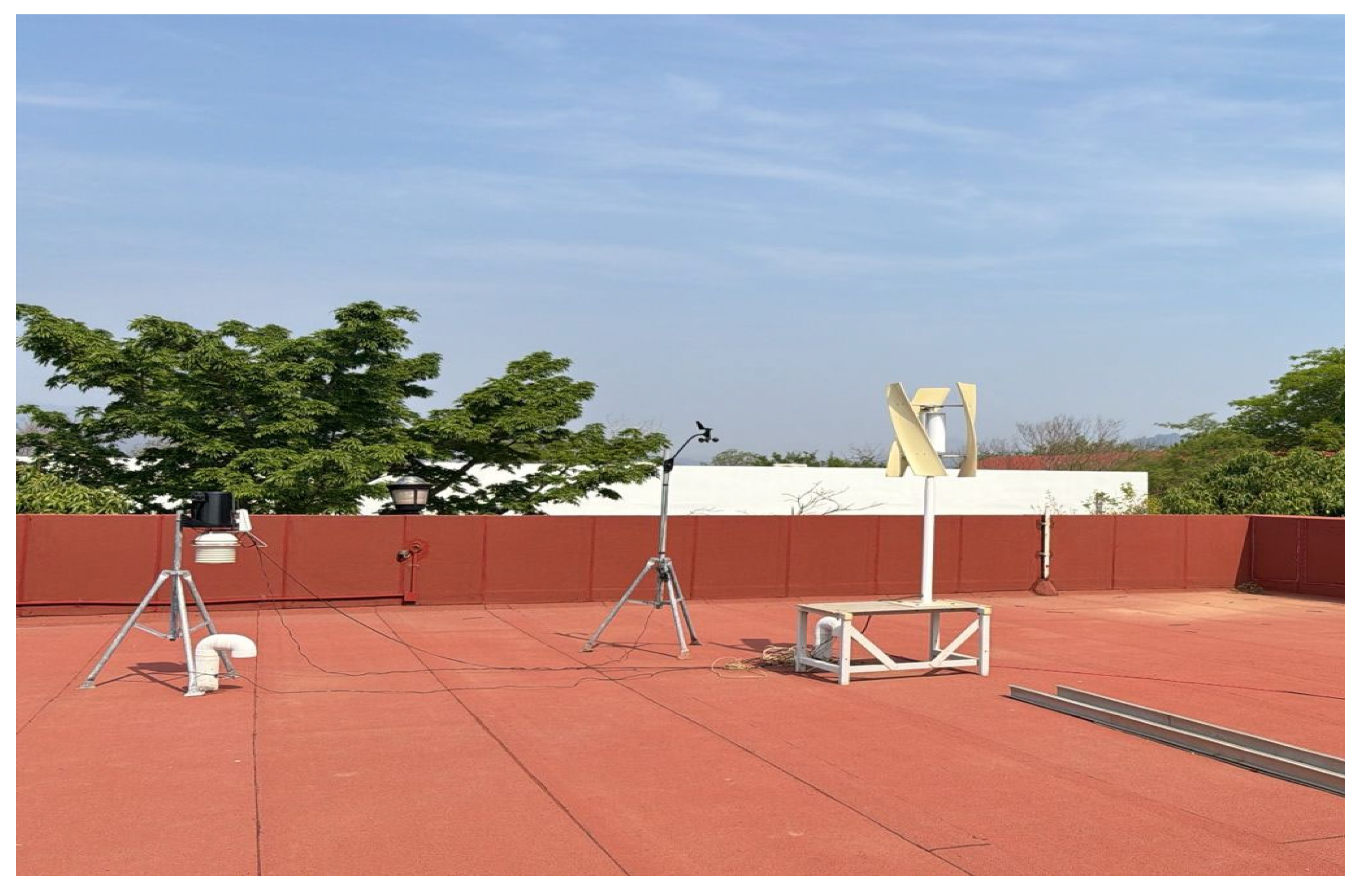
Figure 6 presents the experimental system installed on the rooftop of the research building at the University of the Isthmus. The system consists of a vertical-axis wind turbine (VAWT), meteorological instrumentation, and auxiliary devices for the continuous acquisition of environmental and electrical variables.

The wind turbine operates under real wind exposure conditions and is complemented by meteorological sensors located near the rotor, enabling the simultaneous monitoring of wind speed and environmental variables required for power curve construction.

The experimental configuration also incorporates auxiliary power supply and energy monitoring components integrated within the research platform installed at the site.

3.3. Experimental Bench and Data Acquisition

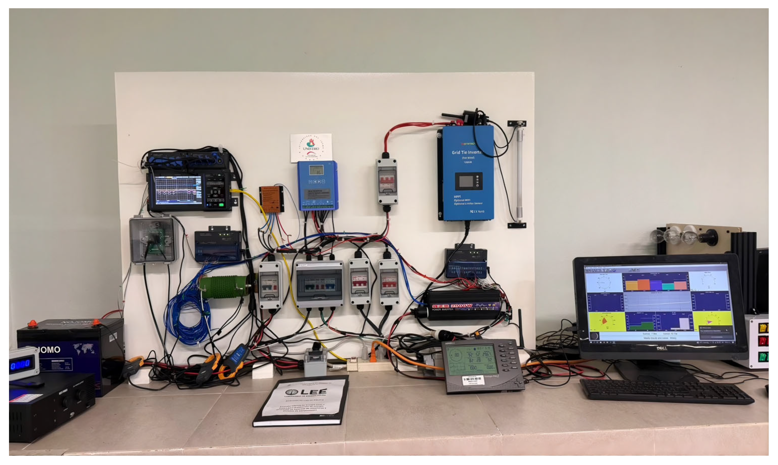
Figure 7 shows the experimental bench and monitoring infrastructure implemented for the acquisition and storage of operational data. The system integrates power electronic converters, protection devices, signal conditioning modules, measurement instrumentation, and a SCADA-based supervision platform intended for real-time recording of the meteorological and electrical variables of the system. The experimental architecture enabled the continuous acquisition of wind speed, generated power, and operational variables, constituting the database used for the evaluation and comparison of the power curve modeling methods.

The measurement instruments employed in the experimental platform were selected to ensure reliable long-term monitoring of both electrical and meteorological variables.

Table 2. Measurement Instruments and Accuracy.

Instrument	Measured	Measurement Range	Accuracy
Hioki PQ3198	Voltage/Power	According to sensor	±0.1 rdg.
Hioki LR8450	Data adquisition	-	16-bit resolution
Hioki CT7731	Current	100 A	±0.3 rdg.
Hioki CT7126	Current	60 A	±0.3 rdg.
Cup Anemometer	Wind speed	0–40 m/s	Mfr. spec.

summarizes the main specifications and measurement accuracies of the sensors and data acquisition devices used in this study. The use of calibrated instrumentation with known performance characteristics contributes to reducing measurement uncertainty and supports the reliability and reproducibility of the experimental dataset employed for power curve modeling and validation.

The SCADA system continuously recorded the electrical and environmental variables required for the present study throughout the measurement campaign. Prior to model development, the acquired dataset was subjected to a quality-control procedure to verify the physical consistency of the recorded measurements.

Table 3. Summary of the SCADA Dataset and Data Quality Verification.

Item	Value
Measurement period	January–December
Sampling interval	1 h
Raw SCADA observations	8760
Data quality verification	0 ≤ Wind Speed ≤ 20 m/s; Power ≥ 0 W
Invalid observations removed	0
Final observations used for modeling	8760

summarizes the main characteristics of the dataset together with the validation criteria applied before the comparative analysis.

As shown in Table 3 all recorded observations satisfied the predefined quality-control criteria. Consequently, the complete dataset of 8760 hourly measurements was retained for model training, testing, and validation, ensuring the consistency and reproducibility of the comparative assessment.

3.4. Wind Resource Characterization

To characterize the wind resource behavior at the experimental site, a statistical analysis of wind speed and wind direction recorded during the study period was carried out.

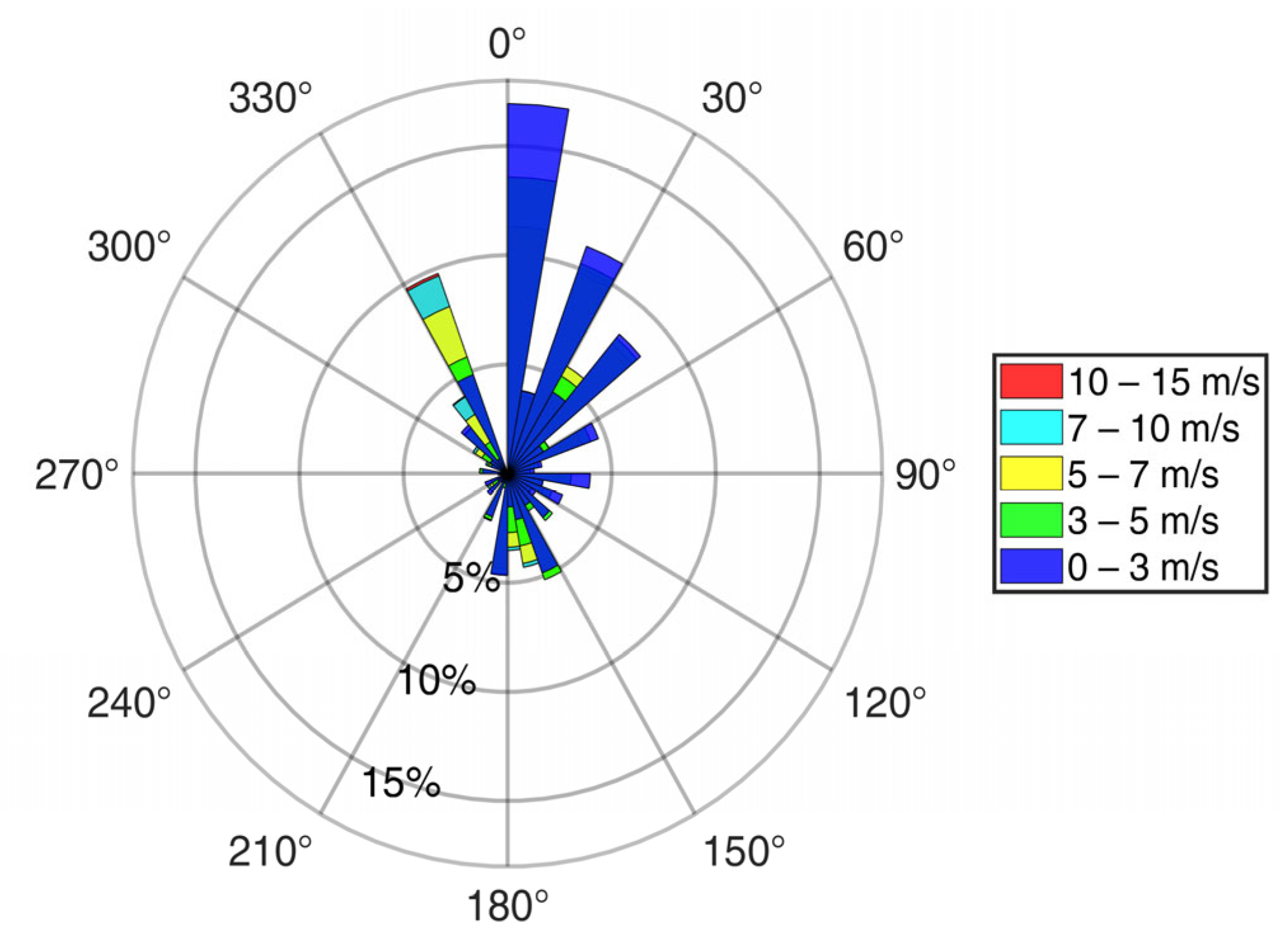
Figure 8 presents the wind rose derived from wind measurements recorded by the SCADA system at the experimental site located in the vicinity of the University of the Isthmus (UNISTMO), in the Isthmus of Tehuantepec region, Oaxaca, Mexico. The wind data were acquired using the anemometer installed above the Graduate Studies building. The angular distribution reveals a marked predominance of winds originating from the northern and northeastern sectors, mainly between 0° and 60°, which is consistent with the characteristic behavior of the Tehuantepec winds, recognized for their high intensity and persistence in this region.

It can be observed that the highest frequency corresponds to the wind speed interval between 0 and 3 m/s, represented in blue, indicating that a large proportion of the records are concentrated within low and moderate wind speed ranges. However, significant contributions are also identified in the 3–5 m/s and 5–7 m/s ranges, particularly for the predominant northern directions. Wind speeds above 7 m/s exhibit a lower relative frequency, although they maintain the same directional trend.

The concentration of frequencies in specific directions reflects the atmospheric channeling effect characteristic of the Isthmus of Tehuantepec, where the geographical configuration and the Chivela Pass favor the accelerated flow of air masses from the Gulf of Mexico toward the Pacific Ocean. This behavior has been widely reported as one of the main factors responsible for the high wind energy potential of the region.

From a quantitative perspective, the wind rose shows that the prevailing wind directions are concentrated between 0° and 60°, while most wind speed observations are distributed within the 0–7 m/s intervals, with progressively lower frequencies at higher wind speeds. These operating conditions are particularly relevant because they correspond to the transition and partial-load regions of the wind turbine power curve, where the relationship between wind speed and generated power is highly nonlinear. Consequently, the experimental dataset provides a representative basis for evaluating the capability of the analytical, parametric, and machine learning models to accurately capture power curve behavior under realistic atmospheric conditions.

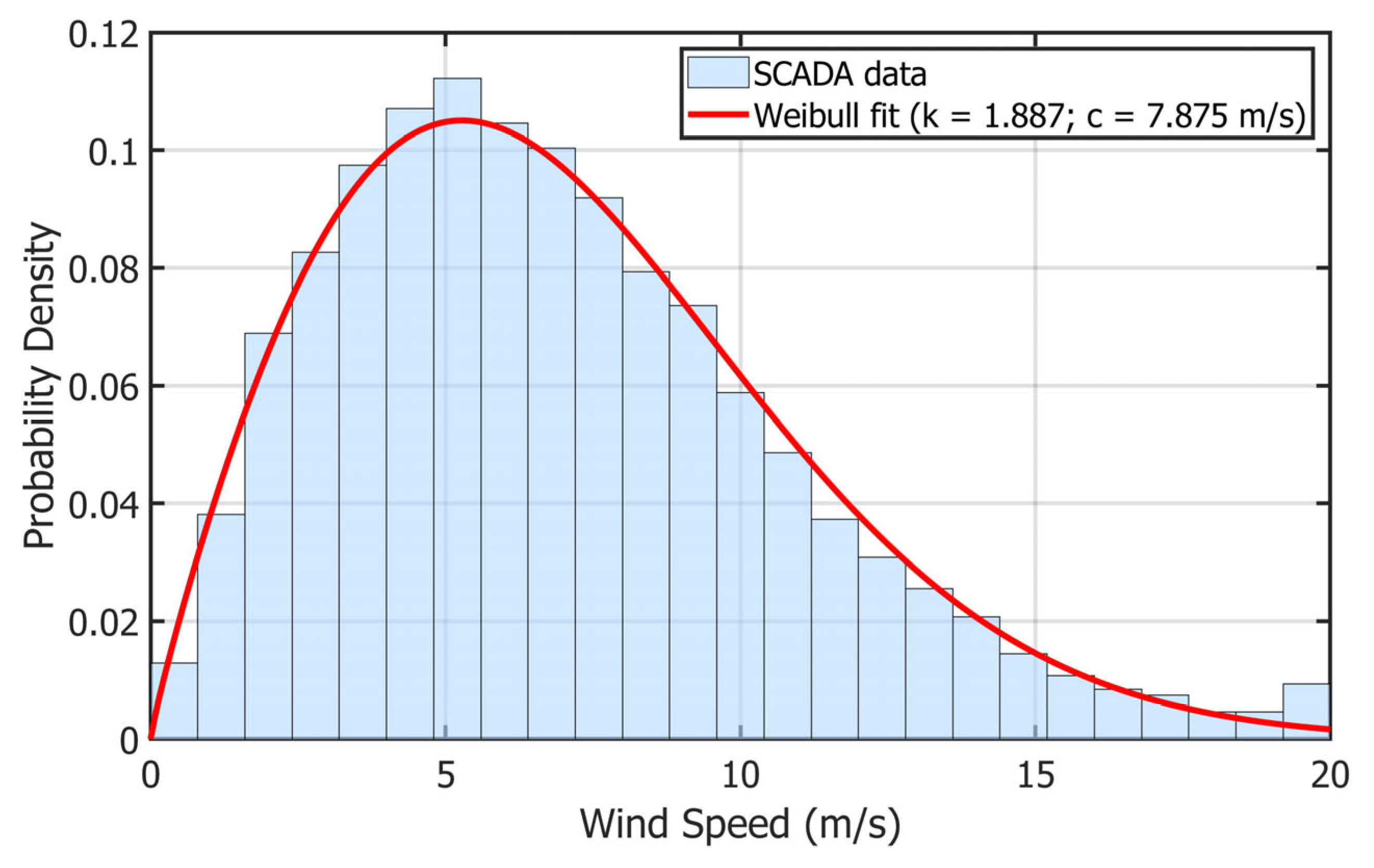
Figure 9 presents the statistical distribution of wind speed obtained from the SCADA monitoring system at the experimental site, together with the fitted Weibull distribution. The wind speed measurements were acquired using the anemometer installed above the Graduate Studies building. The histogram represents the probability density of the wind speeds recorded during the analysis period, whereas the red line corresponds to the Weibull distribution fitted using the maximum likelihood estimation method.

The estimated distribution parameters were k = 1.887 for the shape parameter and c = 7.875 m/s for the scale parameter. The value k < 2 indicates moderate variability of the wind resource and an asymmetric distribution characteristic of wind regimes with noticeable fluctuations, whereas the scale parameter reflects a relatively high characteristic wind speed, consistent with the wind energy potential of the Isthmus of Tehuantepec.

It can be observed that the highest frequency of wind speed occurrence is concentrated approximately between 3 and 9 m/s, reaching a maximum density around 5–6 m/s, indicating that moderate wind speeds predominate during the analyzed period. Furthermore, the distribution exhibits an extended tail toward higher wind speeds, evidencing the occasional occurrence of more intense wind events.

The Weibull fit adequately reproduces the experimental behavior, showing good agreement with the histogram both in the region of maximum probability and in the progressive decrease observed for wind speeds above 10 m/s. This confirms the capability of the Weibull distribution to statistically represent the wind resource at the experimental site.

Furthermore, the low frequency of extreme wind speeds above 15 m/s indicates that the wind turbine operates most of the time within the growth and transition regions of the power curve, a condition that is particularly relevant for the comparative analysis and validation of the different modeling methods evaluated in this study.

3.5. Descriptive Statistical Analysis of the Data

Prior to modeling, a descriptive statistical analysis of the dataset was performed to characterize the behavior of the wind resource and the energy response of the wind turbine at the experimental site.

Table 4. Descriptive Statistics.

Variable	Min	Max	Mean	Std. Dev.
Wind speed (m/s)	0.02	20.00	6.98	3.87
Generated Power (W)	0.00	1650	528.47	537.97
Ambient Temperature (°C)	20.23	33.09	27.00	2.60

presents the main descriptive statistics of the primary variables considered in this study.

The results show that the wind speed at the experimental site presents a mean value of 6.98 m/s, with values ranging from 0.02 m/s to 20.00 m/s, reflecting the variable wind regime characteristic of the Isthmus of Tehuantepec. The generated power exhibits high dispersion, with a standard deviation of 537.97 W, which is consistent with the pulsating nature of the incoming flow in vertical-axis wind turbines.

In the present study, wind speed was intentionally selected as the only predictor variable for all evaluated models. This decision was made to ensure a fair and unbiased comparison among analytical, parametric, statistical, and machine learning approaches by providing exactly the same input information to every model. Although additional variables such as air density, turbulence intensity, wind direction, and atmospheric stability are known to influence the aerodynamic behavior of vertical-axis wind turbines, incorporating these variables would modify the objective of the study from a comparative assessment of modeling methodologies to the development of multivariate predictive models. Therefore, the present work focuses exclusively on evaluating the predictive capability of different power curve modeling techniques under identical input conditions.

3.6. Model Training, Validation, and Hyperparameter Configuration

To ensure a fair and reproducible comparison among all power curve modeling approaches, the experimental dataset was randomly divided into two independent subsets using a fixed random seed (rng = 1). A total of 70% of the observations were assigned to the training dataset, while the remaining 30% were reserved exclusively for model testing and validation. This partitioning strategy ensured that model evaluation was performed using previously unseen data, thereby providing an unbiased assessment of predictive performance.

The training dataset was used to estimate the parameters of all power curve models, including the Manufacturer’s Curve adaptation, BEMT, Polynomial Regression, Logistic Regression, Random Forest (RF), Gaussian Process Regression (GPR), and Kernel Density Estimation (KDE). The testing dataset was employed solely to evaluate the predictive capability of each model. Consequently, all reported performance metrics, including the Root Mean Square Error (RMSE), Mean Absolute Error (MAE) and Coefficient of Determination (R²), were computed exclusively from the independent testing dataset.

A hold-out validation strategy was adopted by randomly partitioning the dataset into independent training (70%) and testing (30%) subsets. This approach was selected to provide a consistent and reproducible evaluation framework for all compared models using previously unseen observations.

For the machine learning models, the Random Forest regression model was implemented using MATLAB’s TreeBagger function with 300 regression trees, bootstrap aggregation, out-of-bag (OOB) prediction enabled, and a minimum leaf size of five observations. Since wind speed was the only predictor variable considered in this study, it was used at every node split during tree construction, while tree depth was automatically determined according to the stopping criterion. The Gaussian Process Regression (GPR) model employed a Squared Exponential kernel with standardized input data, and the kernel hyperparameters, including the characteristic length scale and signal variance, were automatically optimized during model training by maximizing the marginal likelihood. For the Kernel Density Estimation (KDE) model, a Gaussian kernel with a bandwidth of 0.5 m/s was adopted to estimate the conditional probability density of wind power generation. The configuration parameters of all evaluated power curve models are summarized in

Table 5. Configuration Parameters of the Evaluated Power Curve Models.

Model	Configuration
Manufacturer	Commercial manufacturer’s power curve used as reference.
BEMT	ρ = 1.225 kg/m3; Rotor radius = 0.55 m; Swept area = 1.80 m2; Cp,max = 0.40; Cut-in wind speed = 2.5 m/s; Rated wind speed = 11 m/s.
Polynomial	Third-order polynomial regression fitted using the training dataset.
Logistic	Three-parameter logistic regression initialized with [Pmax, 0.8, 9]; parameters estimated by nonlinear least squares.
Random Forest	300 regression trees; Bootstrap aggregation; Minimum leaf size = 5; One predictor sampled per split; Out-of-Bag prediction enabled.
Gaussian Process Regression	Squared Exponential kernel; Standardized input data; Hyperparameters optimized by maximizing the marginal likelihood.
Kernel Density Estimation	Gaussian kernel; Bandwidth = 0.5 m/s; Conditional estimation based on wind speed observations.

.

Although chronological data partitioning or blocked cross-validation can be advantageous for strongly autocorrelated SCADA time-series, the primary objective of the present work was to compare the predictive capability of different power curve modeling approaches under a common and reproducible evaluation framework. Therefore, the same fixed random hold-out partition was consistently applied to all evaluated models under identical experimental conditions. Accordingly, a single fixed random hold-out partition was adopted to ensure a fair, consistent, and fully reproducible comparison among all evaluated models.

4. Results

This section presents the comparative analysis of the different models employed for wind turbine power curve estimation using real SCADA data. The evaluation is performed with the objective of identifying the capability of each method to reproduce the physical behavior of the system, particularly within the cut-in, transition, and rated power operating regions.

4.1. Manufacturer-Provided Power Curve

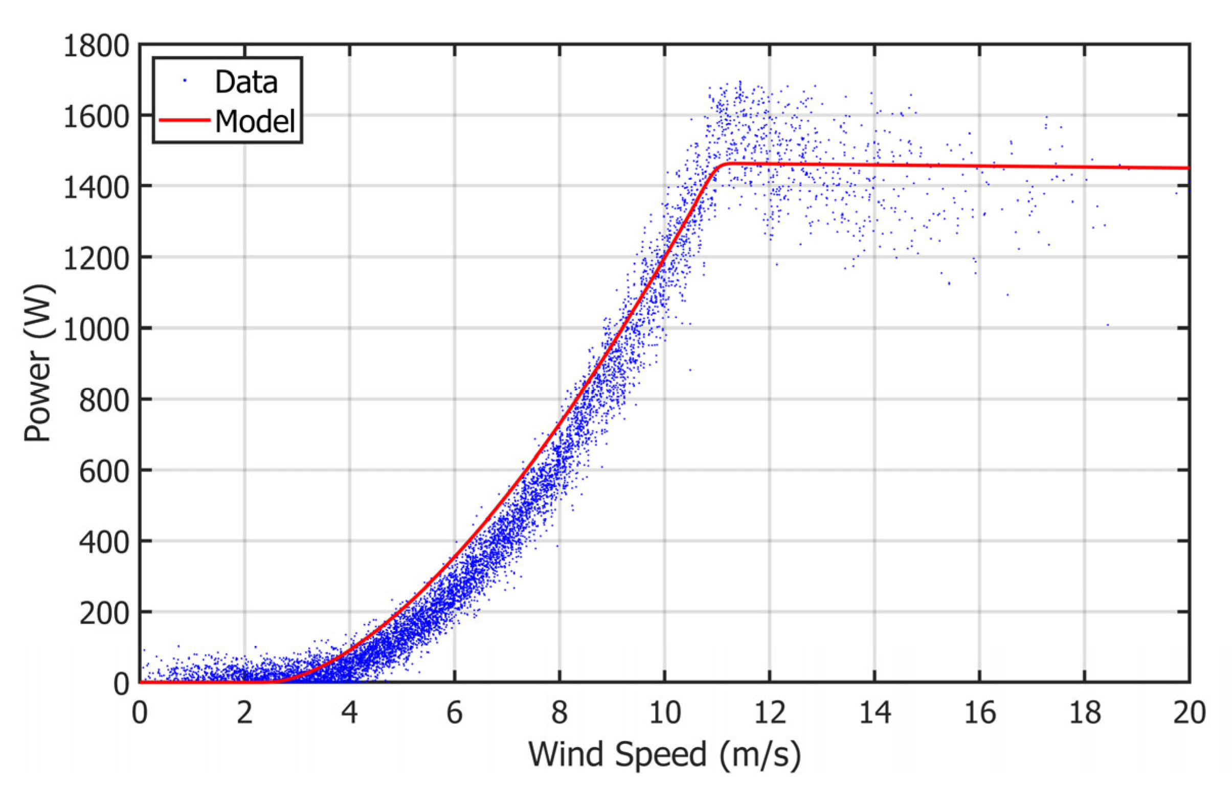
The manufacturer-provided power curve is used as a reference to establish a baseline representation of turbine performance. Figure 10 shows the comparison between the power curve provided by the manufacturer and the scatter plot obtained from the experimental wind speed and generated power data. It can be observed that the power output remains close to zero for wind speeds below approximately 3 m/s, corresponding to the cut-in region of the wind turbine. Subsequently, the power output increases progressively between 4 and 10 m/s, following a nonlinear trend characteristic of the aerodynamic energy conversion process.

Rated power is reached at approximately 11 m/s, with values close to 1450 W, remaining nearly constant up to wind speeds close to 20 m/s. Likewise, the scatter plot shows a higher concentration of observations within the 4–8 m/s interval, reflecting the predominant wind speed distribution recorded at the study site. For wind speeds above the rated condition, a greater dispersion of the experimental data around the manufacturer power curve is observed, associated with operational variations and environmental conditions present during data acquisition.

In summary, the manufacturer power curve provides a simplified and idealized representation that is insufficient for accurate performance analysis and power curve modeling under real operating conditions.

4.2. BEMT Model

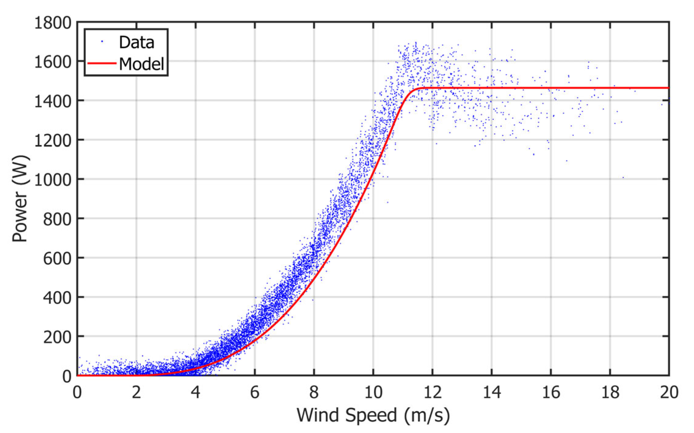
Figure 11 presents the power curve estimated using the BEMT method and its comparison with the experimental scatter plot obtained at the study site. It can be observed that the model adequately reproduces the characteristic aerodynamic behavior of the wind turbine, identifying three main operating regions: an initial region with practically null power generation for wind speeds below approximately 3 m/s, a progressive power increase region between 4 and 10 m/s, and a stabilization region associated with rated power operation.

The power increase predicted by the BEMT model exhibits a continuous trend that is physically consistent with the wind kinetic energy extraction process, reaching values close to 1450 W at approximately 11 m/s. Subsequently, the curve remains nearly constant up to 20 m/s, representing the rated power operating condition of the system.

Likewise, the experimental distribution exhibits a higher density of observations within the 4–8 m/s range, whereas a wider dispersion with respect to the theoretical model is observed for wind speeds above 12 m/s. This behavior may be associated with operational variations, turbulence effects, and environmental conditions recorded during data acquisition.

The BEMT model enabled the representation of the physical behavior of the wind turbine through aerodynamic principles, constituting a theoretical reference for comparison with the statistical and machine learning methods implemented in this study.

4.3. Polynomial Model

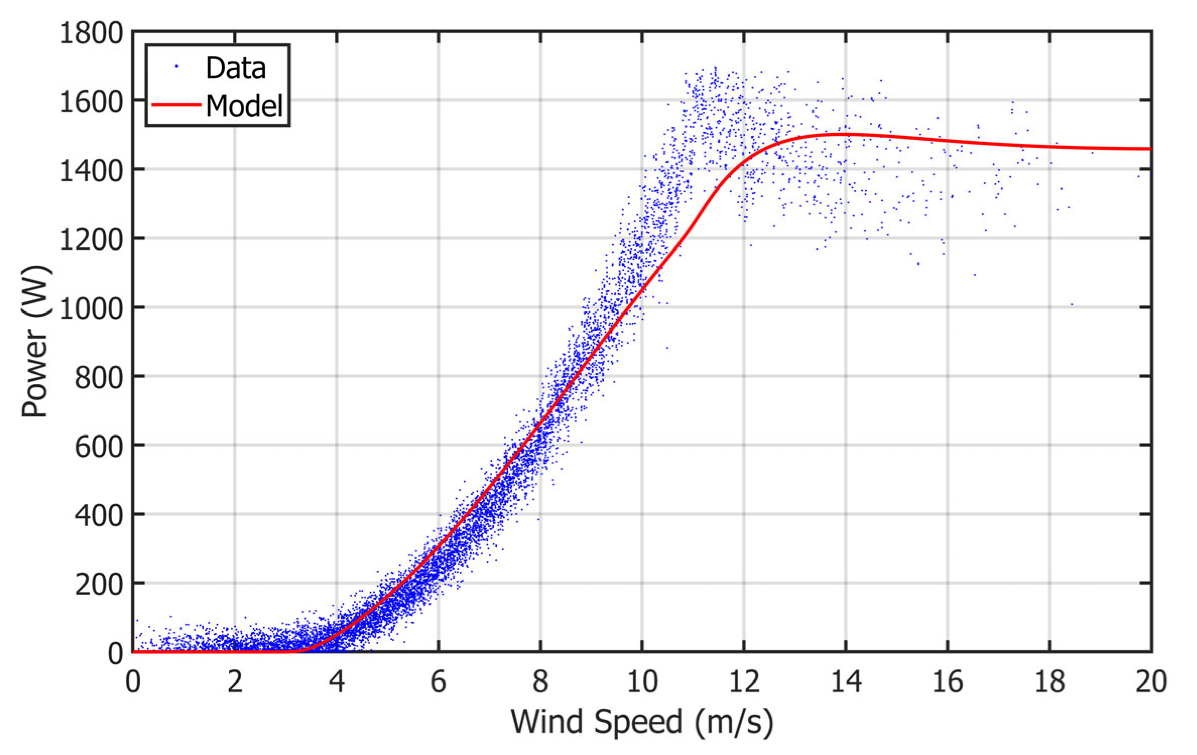
Figure 12 presents the power curve estimated using the polynomial fitting approach and its comparison with the experimental data recorded at the study site. It can be observed that the model adequately reproduces the increasing trend of power within the operating region approximately between 4 and 10 m/s, following the main distribution of the scatter plot.

The polynomial curve describes the progressive increase in power associated with the increase in wind speed, reaching values close to the rated power at approximately 12–13 m/s. Subsequently, the model exhibits a slight overestimation in the transition region followed by a gradual reduction in power for wind speeds above 14 m/s, evidencing the characteristic behavior of the applied empirical fitting approach.

Likewise, the highest concentration of experimental observations is located within the 4–8 m/s range, whereas a greater dispersion of the data with respect to the fitted curve is identified for higher wind speeds. This behavior reflects the operational variability observed in the system and the environmental conditions recorded during data acquisition.

In contrast to the BEMT model, which is founded on aerodynamic principles, the polynomial model represents an empirical approximation directly derived from the observed relationship between wind speed and power generation.

4.4. Logistic Model

Figure 13 shows the power curve estimated using the logistic model and its comparison with the experimental data obtained at the study site. It can be observed that the model adequately reproduces the nonlinear relationship between wind speed and generated power, describing a sigmoidal response characteristic of wind power curves.

For wind speeds below approximately 3 m/s, power generation remains close to zero, corresponding to the cut-in region of the wind turbine. Subsequently, the model exhibits a progressive increase between 4 and 10 m/s, coinciding with the highest density of experimental observations recorded in the scatter plot.

The transition region develops around 8–11 m/s, where the slope of the curve reaches its maximum growth, until approaching the rated power of approximately 1450 W. For wind speeds above 12 m/s, the curve exhibits a stabilization trend, remaining nearly constant up to 20 m/s and reproducing the expected rated operating behavior.

Likewise, a greater dispersion of the experimental data is observed for higher wind speeds, whereas the model maintains a smooth and continuous transition, evidencing the capability of the logistic fitting approach to represent the overall behavior of the power curve.

In contrast to the polynomial model, the logistic model incorporates a sigmoidal representation capable of continuously describing the cut-in, growth, and stabilization regions of power generation.

4.5. Gaussian Process Regression Model

Figure 14 shows the power curve estimated using the Gaussian Process Regression (GPR) model and its comparison with the experimental data obtained at the study site. It can be observed that the model adequately reproduces the nonlinear behavior of the wind turbine, describing the evolution of generated power from the cut-in region to the rated operating zone.

For wind speeds below approximately 3 m/s, power generation remains close to zero, corresponding to the cut-in wind speed of the wind turbine. Subsequently, between 4 and 10 m/s, the curve exhibits a progressive increase in power, following the predominant distribution of experimental observations recorded within this wind speed interval.

Likewise, the GPR model exhibits a slight overestimation around 11–12 m/s, reaching values close to 1500 W before converging toward the rated operating region. For wind speeds above 13 m/s, the curve shows stabilization near 1450 W, reproducing the expected turbine behavior under rated operating conditions.

4.6. Random Forest Model

Figure 15 presents the power curve estimated using the Random Forest model and its comparison with the experimental scatter plot obtained at the study site. It can be observed that the model adequately reproduces the overall behavior of the wind turbine, describing the transition from the cut-in region to the rated power operating condition.

For wind speeds below approximately 3 m/s, the generated power remains close to zero, whereas a progressive increase associated with the main energy conversion region is identified between 4 and 10 m/s. Within this interval, the model consistently follows the predominant distribution of the experimental data.

Likewise, the Random Forest model exhibits a slight overestimation as the turbine approaches the rated operating condition (approximately 11–12 m/s), reaching values close to 1500 W. Subsequently, the curve gradually converges toward a stable operating condition near the rated power of approximately 1450 W for wind speeds above 13 m/s.

The scatter plot evidences a higher concentration of observations within the 4–8 m/s range, whereas a wider dispersion with respect to the fitted curve is observed for higher wind speeds. Nevertheless, the model maintains a continuous and stable representation of the overall behavior of the power curve throughout the entire analyzed interval.

The Random Forest model enabled the representation of the relationship between wind speed and generated power through a machine learning approach based on ensemble decision trees, capturing the nonlinear nature of the system.

4.7. Kernel Density Estimation Model

Figure 16 shows the power curve estimated using the Kernel Density Estimation (KDE) method and its comparison with the experimental scatter plot obtained at the study site. It can be observed that the model adequately reproduces the nonlinear relationship between wind speed and generated power, following the main trend of the experimental data.

For wind speeds below approximately 3 m/s, the power output remains close to zero, corresponding to the cut-in region of the wind turbine. Subsequently, between 4 and 10 m/s, the curve exhibits a progressive increase in power, coinciding with the region of highest concentration of experimental observations.

Likewise, the KDE model exhibits a smooth approach to the rated operating condition, reaching values close to 1500 W around 11–12 m/s. Subsequently, the curve gradually converges toward a stable operating condition near 1450 W for wind speeds above 13 m/s, maintaining a slight decrease before stabilization.

The experimental distribution evidences a higher data density within the interval between 4 and 8 m/s, whereas a greater dispersion around the fitted curve is observed for higher wind speeds. Nevertheless, the KDE model maintains a continuous representation of the power curve and preserves the overall trend observed experimentally.

The KDE method enabled the estimation of the power curve through a non-parametric approach based on kernel functions, providing a smooth representation of the experimental data distribution.

4.8. Global Comparison of Models

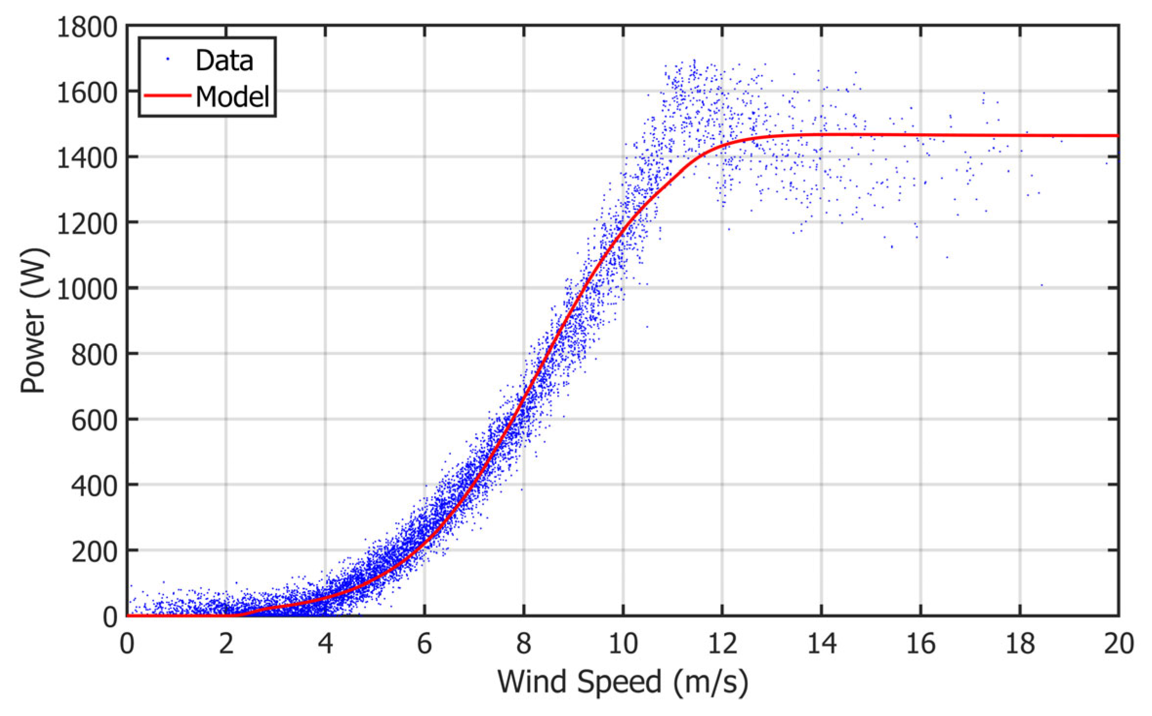
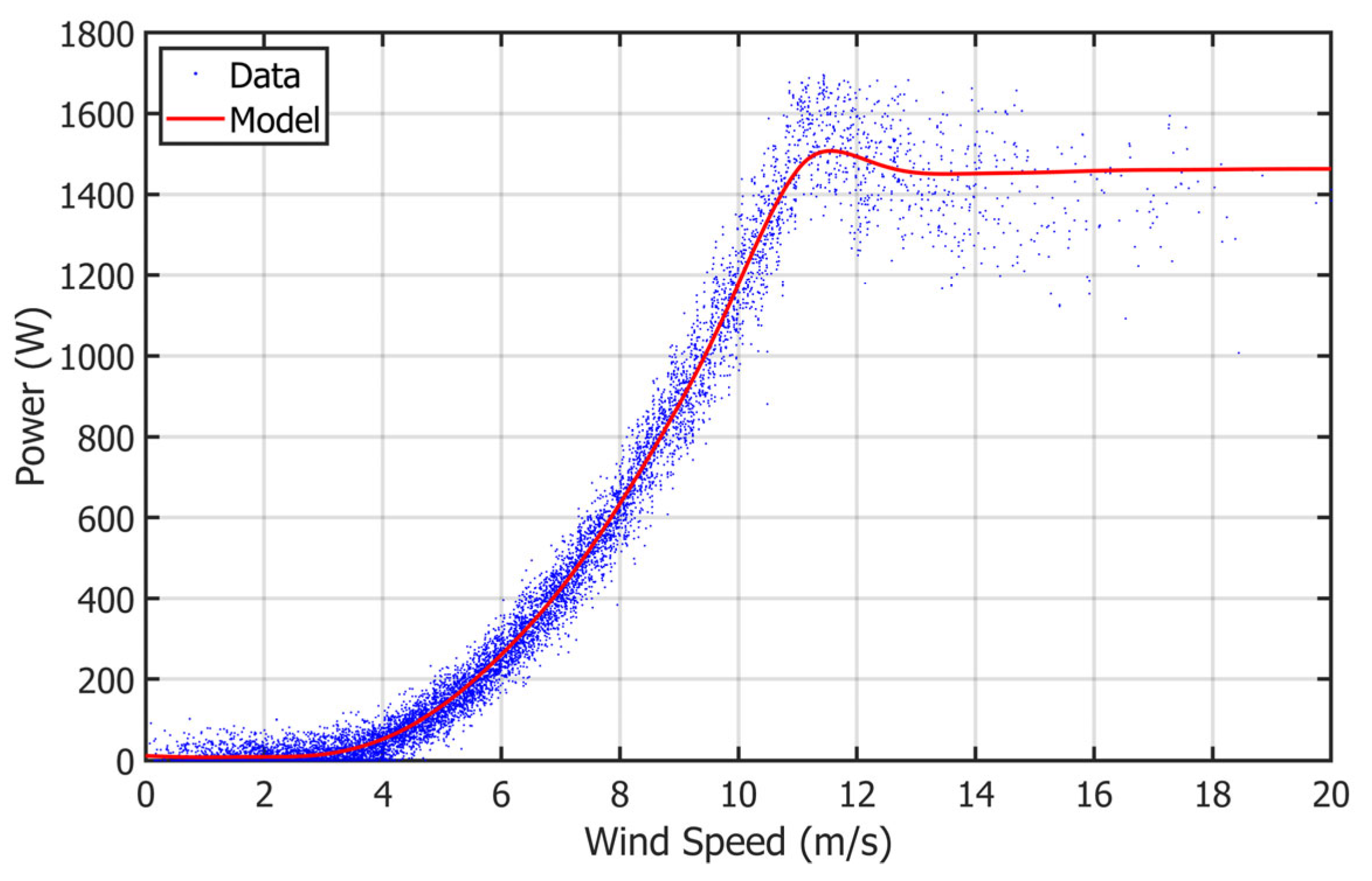
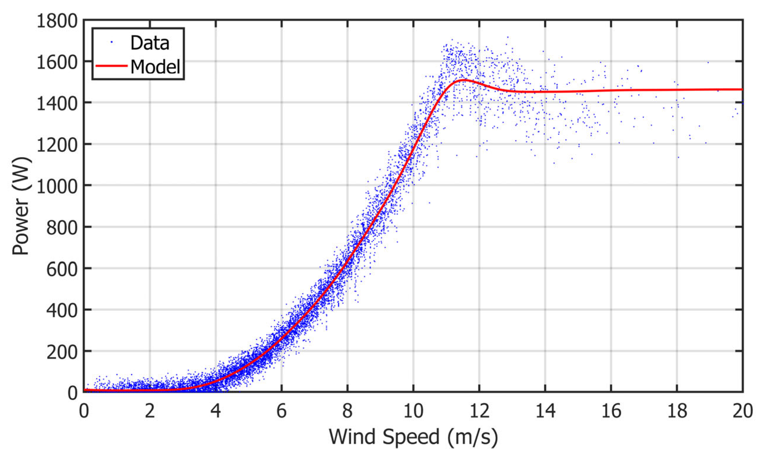
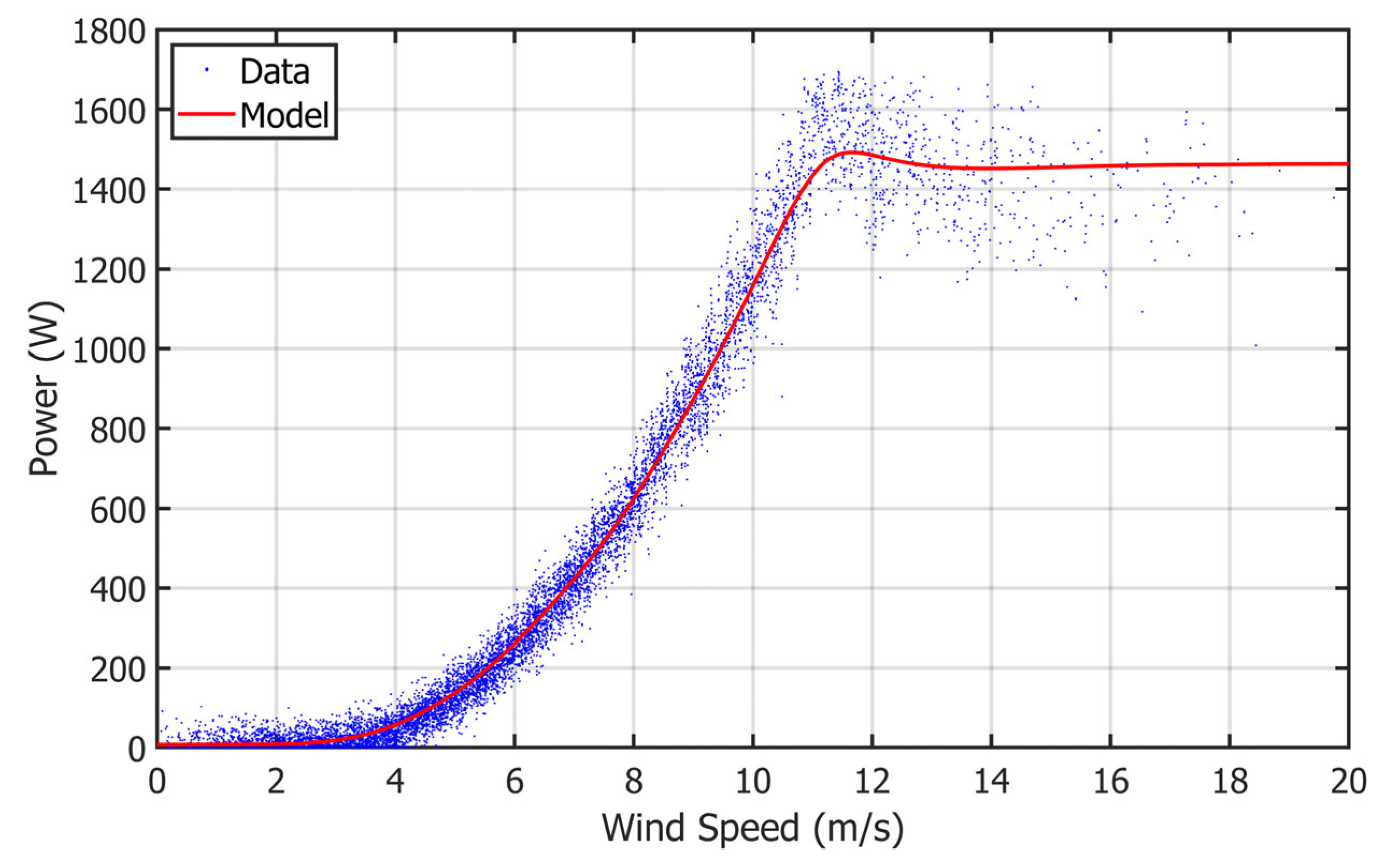
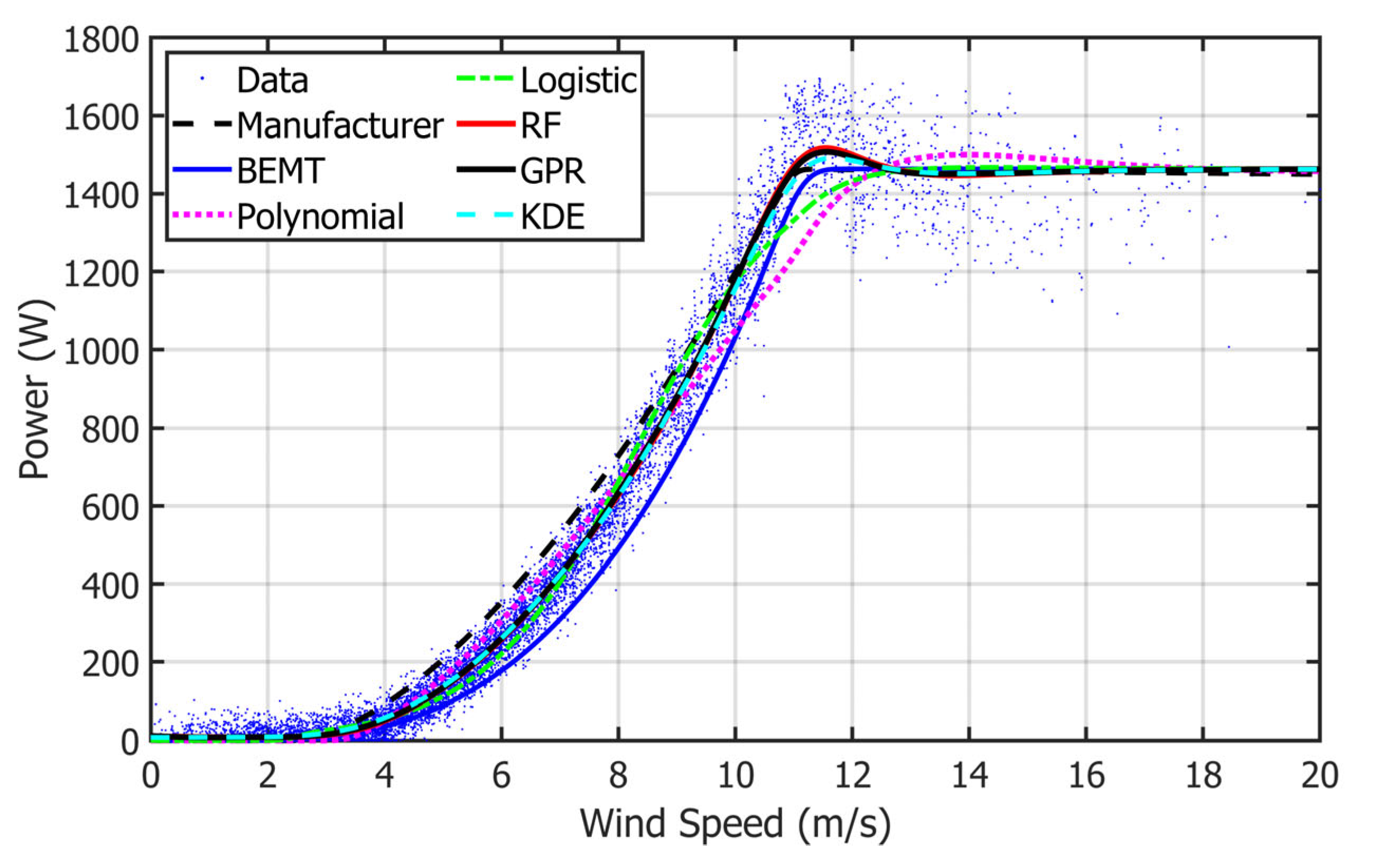
Figure 17 presents the comparison between the manufacturer power curve and the models developed using BEMT, polynomial fitting, logistic model, Random Forest (RF), Gaussian Process Regression (GPR), and Kernel Density Estimation (KDE), together with the experimental scatter plot obtained at the study site.

It can be observed that all methods reproduce the overall behavior of the wind turbine power curve, identifying the cut-in region for wind speeds below approximately 3 m/s, a progressive increase region between 4 and 10 m/s, and a stabilization zone corresponding to the rated power of approximately 1450 W.

The manufacturer model exhibits an earlier increase in power output and a continuous evolution until reaching the rated operating condition. In contrast, the BEMT model shows a steeper slope within the growth region, slightly shifting the power increase toward higher wind speeds. The polynomial fitting approach presents a smoother increase in power output and a gradual approach toward the rated operating condition.

Likewise, the logistic, RF, GPR, and KDE models show better agreement with the experimental scatter plot within the partial-load operating region. As the turbine approaches the rated operating condition (approximately 11–12 m/s), the RF, GPR, and KDE models exhibit a slight overestimation before converging toward the rated power, reproducing more closely the main distribution of the experimental observations.

The scatter plot evidences a higher data density within the 4–8 m/s range, whereas a greater experimental dispersion around the estimated curves is observed for wind speeds above 12 m/s. Nevertheless, all models maintain a consistent representation of the overall turbine behavior throughout the analyzed interval.

The differences observed among the models were subsequently evaluated using statistical performance indicators, including RMSE, MAE, and R², with the objective of quantifying the predictive capability of each approach.

4.9. Quantitative Performance Evaluation

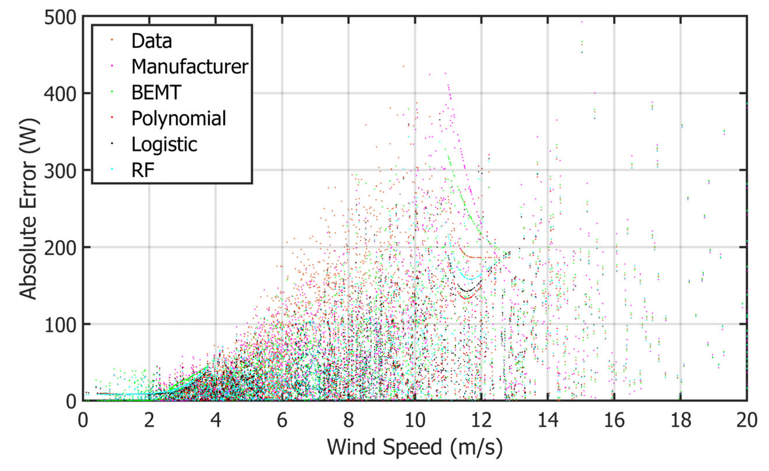
Figure 18 shows the distribution of the absolute error associated with the different power curve estimation methods as a function of wind speed. It can be observed that the errors remain relatively low for wind speeds below approximately 4 m/s, since the generated power in this region is close to zero.

Between 4 and 10 m/s, a progressive increase in the absolute error is identified as generated power and the dispersion of the experimental data increase. Within this interval, the models exhibit differences in their fitting capability with respect to the experimental scatter plot. The polynomial method shows a greater error dispersion, particularly around 10–12 m/s, where values exceeding 400 W are observed, associated with the approach to the rated operating condition.

On the other hand, the logistic, Random Forest (RF), and BEMT models show a more concentrated error distribution around intermediate values, maintaining a more stable behavior compared to the polynomial fitting approach. Likewise, it is observed that the error dispersion increases for wind speeds above 12 m/s, where the experimental variability of generated power is higher.

The figure also evidences that the highest concentration of observations is located within the 4–8 m/s range, coinciding with the predominant wind speed interval recorded at the study site. In general, machine learning-based methods and probabilistic approaches exhibit a more uniform error distribution compared to traditional empirical models.

Table 6. Comparison of Statistical Performance.

Methods	RMSE (W)	RMSE (%)	MAE (W)	MAE (%)	${\mathbf{R}}^2$
Manufacturer	99.925	6.66	76.539	5.10	0.96606
BEMT	112.800	7.52	81.856	5.46	0.95674
Polynomial	103.010	6.87	65.990	4.40	0.96393
Logistic	87.561	5.84	57.171	3.81	0.97394
RF	74.007	4.93	48.122	3.21	0.98138
GPR	74.430	4.96	48.511	3.23	0.98117
KDE	75.479	5.03	49.439	3.30	0.98063

Note: Normalized RMSE (%) and MAE (%) were calculated with respect to the rated turbine power of 1500 W.

presents the statistical performance obtained for the evaluated methods, including the manufacturer power curve, the BEMT model, polynomial fitting, logistic model, Random Forest (RF), Gaussian Process Regression (GPR), and Kernel Density Estimation (KDE). The evaluation was performed using the RMSE, MAE, and coefficient of determination (R²) metrics.

The Random Forest (RF) model achieved the lowest RMSE (74.007 W), MAE (48.122 W), and the highest coefficient of determination (R² = 0.9813) among the evaluated methods. However, the differences with the Gaussian Process Regression (GPR) and Kernel Density Estimation (KDE) models were relatively small, indicating that these three machine learning approaches exhibited comparable predictive performance under the evaluated operating conditions.

Similarly, the Gaussian Process Regression (GPR) model exhibited comparable performance, with RMSE = 74.430 W, MAE = 48.511 W, and R² = 0.98117, indicating that probabilistic approaches enable an adequate representation of the uncertainty and dispersion present in operational data. Likewise, the KDE method showed competitive results (RMSE = 75.479 W, MAE = 49.439 W, and R² = 0.98063), confirming its potential as a non-parametric alternative for power curve estimation.

The logistic model exhibited intermediate performance, achieving RMSE = 87.561 W and R² = 0.97394. Although the model adequately reproduced the characteristic sigmoidal shape of the wind power curve, its simplified functional structure limited the representation of local variations as the turbine approached the rated operating condition.

On the other hand, the manufacturer power curve and the BEMT model showed higher errors compared to the machine learning-based methods. The manufacturer power curve yielded RMSE = 99.925 and R² = 0.96606, evidencing the differences between the ideal operating conditions considered by the manufacturer and the real operating conditions observed at the study site.

The BEMT model exhibited the lowest predictive performance among the evaluated methods (RMSE = 112.800 W, MAE = 81. 856 W, and R² = 0.95674). This behavior may be attributed to the aerodynamic simplifications inherent to the model and to its limited capability to fully represent the specific operating conditions of the study site.

The polynomial fitting approach achieved slightly better results than the BEMT model (RMSE = 103.010 W and R² = 0.96393); however, it exhibited larger deviations compared to the machine learning-based models, particularly as the turbine approached the rated operating condition.

In general, the machine learning-based approaches (RF, GPR, and KDE) consistently produced lower prediction errors than the conventional analytical and empirical models evaluated in this study. Among these methods, the Random Forest model achieved the lowest observed error metrics; however, its performance was comparable to that of the GPR and KDE models. Therefore, the results should be interpreted as a comparative assessment of predictive performance rather than evidence of statistical superiority among the machine learning approaches.

The relatively small differences between the RMSE and MAE values across all evaluated models indicate that the prediction errors are reasonably homogeneous and are not dominated by a small number of extreme residuals. This behavior is consistent with the data quality verification procedure, which confirmed the physical consistency of the complete SCADA dataset prior to model training and evaluation. Although a formal residual normality analysis was beyond the scope of this comparative study, the RMSE and MAE values suggest that no model was disproportionately affected by extreme prediction errors.

Although the quantitative performance metrics demonstrate the predictive capability of the evaluated models,

Table 7. Comparison of Methods.

Methods	Operation	Advantages	Disadvantages	Performance
Manufacturer Power Curve	Based on ideal operating conditions	Easy implementations; serves as a baseline reference; widely used in technical specifications	Does not consider turbulence, aging effects, mechanical losses, or actual site operating conditions	Exhibited evident discrepancies with respect to the measured scatter plot, particularly within the transition (partial-load) region (4–10 m/s) and at high wind speeds
BEMT	Based on momentum theory and blade element theory	Represents the physical principles of energy conversion; useful for aerodynamic simulations	Sensitive to geometric parameters and model simplifications; limited capability to represent the actual variability of SCADA data	Showed a behavior consistent with the turbine physics, although with higher errors at medium and high wind speeds
Polynomial	Fits a polynomial function to the experimental power data	Simple implementation; low computational cost	Prone to overfitting or loss of stability in extreme regions	Reasonably fitted the intermediate region, but exhibited significant deviations near rated power
Logistic	Uses a sigmoidal function to represent the gradual increase in power up to rated saturation	Smooth and physically consistent curve; good representation of the power increase region	Lower flexibility for highly nonlinear behaviors	Significantly improved the performance compared to the polynomial model and adequately represented the saturation region
GPR	Based on kernel functions and statistical correlation	High accuracy; captures uncertainty and complex nonlinearities	Higher computational cost; sensitive to kernel selection	Exhibited excellent agreement with the experimental data cloud and high stability throughout the entire operating region
RF	Ensemble of decision trees based on supervised learning	Robust to noise; excellent predictive capability; good generalization	Lower physical interpretability	Achieved the best overall performance and the lowest error dispersion
KDE	Estimates the power distribution using kernel functions and local data weighting	Represents complex distributions; provides good statistical smoothness	Dependent on the selected bandwidth	Exhibited stable behavior and results comparable to GPR and RF.

provides a qualitative comparison of the methods, summarizing their operating principles, key advantages, limitations, and observed performance.

4.10. Error Analysis as a Function of Wind Speed

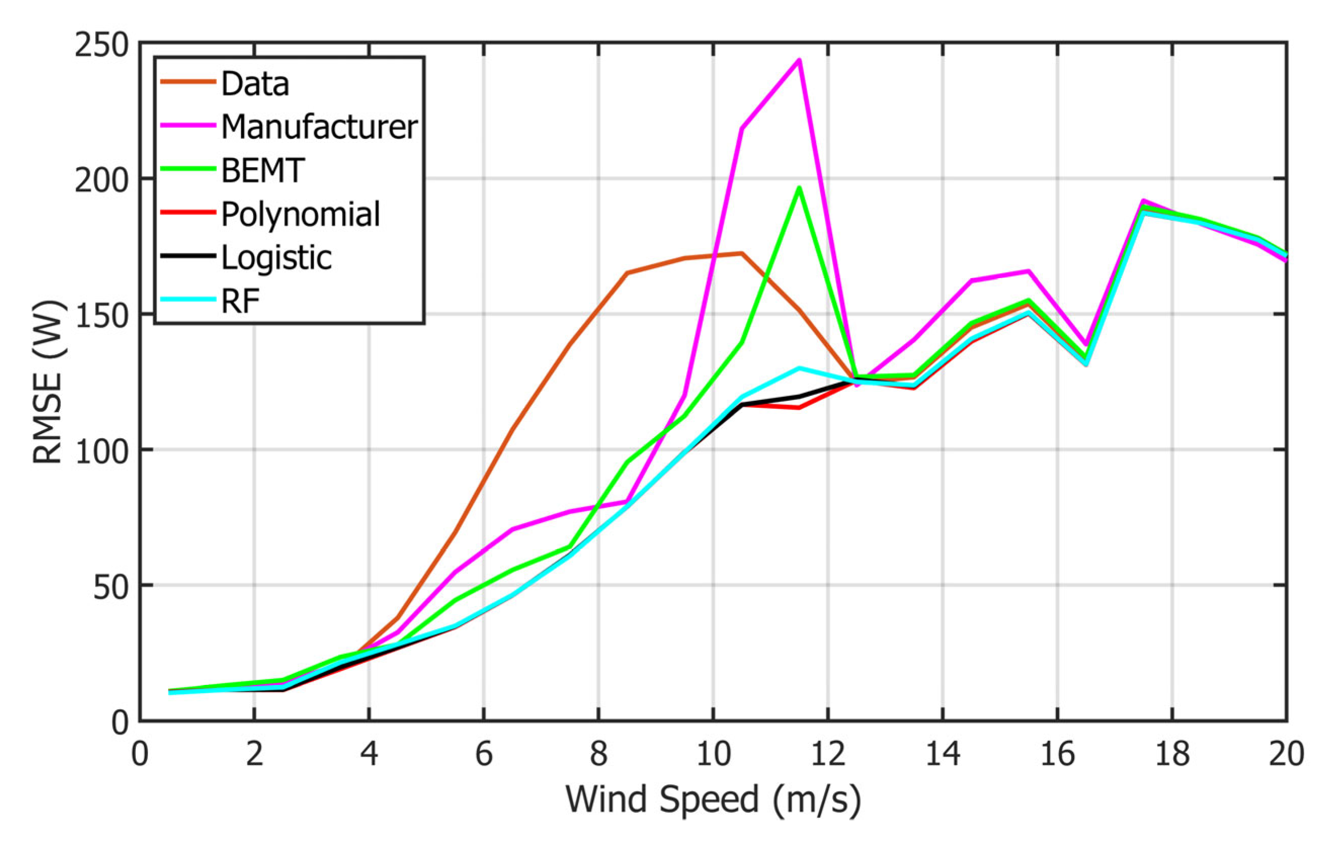
Figure 19 presents the variation in the Root Mean Square Error (RMSE) as a function of wind speed for the different methods employed in power curve estimation, including the manufacturer power curve, BEMT, polynomial fitting, logistic model, and Random Forest (RF).

It can be observed that the RMSE increases progressively with wind speed, particularly within the partial-load operating region (approximately 4–10 m/s), where the generated power increases rapidly with wind speed. The pronounced error peak observed as the turbine approaches the rated operating condition (approximately 10–12 m/s) is associated with increasingly complex aerodynamic behavior rather than with data sparsity. In this operating region, the turbine experiences rapid variations in aerodynamic efficiency caused by continuously changing angles of attack, dynamic stall phenomena, and wake interactions. These effects produce greater stochastic variability in the measured power output, making the relationship between wind speed and generated power more difficult to represent accurately. Consequently, all evaluated models exhibit their highest prediction errors as the turbine approaches the rated operating condition.

The manufacturer power curve exhibits the highest error values, reaching approximately 245 W around 11–12 m/s, evidencing a lower capability to represent real operating conditions with respect to the measured data. Similarly, the BEMT model shows a significant increase in error, with values close to 200 W within the same wind speed region.

On the other hand, the logistic, Random Forest (RF), and polynomial fitting models exhibit relatively lower RMSE values and a more stable behavior, remaining around 115–130 W as the turbine approaches the rated operating condition. In particular, the RF model exhibits the lowest error variability throughout a large portion of the analyzed wind speed range. This behavior further indicates that data-driven models are more capable of adapting to the highly nonlinear aerodynamic conditions occurring as the turbine approaches the rated operating condition, where deterministic analytical models experience greater prediction uncertainty.

Likewise, for wind speeds above 12 m/s, the errors tend to stabilize around 125–190 W, coinciding with the rated power region where the power curve exhibits lower variation in electrical generation. However, localized increases are observed for wind speeds close to 17–18 m/s, associated with the lower density of experimental observations and the dispersion present in the operational data.

In general terms, the figure demonstrates that machine learning-based methods exhibit a more stable response and lower errors compared to traditional analytical and empirical approaches, particularly within the partial-load operating region of the power curve.

5. Discussion

The results obtained in this study confirm that the selection of an appropriate modeling approach is essential for accurately representing the power curve of a vertical-axis wind turbine (VAWT) under real operating conditions. The discrepancies observed between the manufacturer power curve and the measured SCADA data highlight the limitations of standardized power curves, which are generally derived under controlled conditions and do not consider site-specific variability, turbulence intensity, or atmospheric effects [12,18,27]. This behavior is particularly evident in the transition and rated regions, where the dispersion of the measured data increases significantly.

Parametric models, such as polynomial and logistic formulations, provide a better approximation compared to the manufacturer power curve, particularly in the sub-rated region. However, their performance remains limited by their predefined mathematical structure. Polynomial models tend to exhibit limitations in highly nonlinear regions, often leading to overfitting or reduced generalization capability, as previously reported in the literature [35,36,37]. This behavior is mainly attributed to the global nature of polynomial functions, which attempt to represent the entire power curve using a single mathematical expression. Consequently, local variations associated with turbulence, rapid changes in aerodynamic efficiency, and the partial-load operating region cannot be accurately represented without increasing the polynomial order, which may introduce overfitting and reduce model robustness. In contrast, the logistic model provides a smoother transition between the partial-load and rated operating regions due to its sigmoidal nature, resulting in better agreement with the overall shape of the power curve. Nevertheless, both approaches fail to fully capture the inherent variability of SCADA data, particularly in regions with high dispersion, because they are constrained by predefined functional forms that cannot adapt locally to stochastic fluctuations under real operating conditions.

Non-parametric and machine learning-based models, including Random Forest (RF) and Gaussian Process Regression (GPR), demonstrated superior predictive performance with respect to the manufacturer reference, parametric models, and the conventional BEMT baseline across all evaluated metrics. This superior performance can be attributed to their ability to learn complex nonlinear relationships directly from experimental data without relying on predefined functional forms. Although RF and GPR are based on fundamentally different mathematical principles, both models are highly flexible non-parametric approaches capable of accurately approximating the nonlinear relationship between wind speed and power output. Because wind speed was the only predictor variable considered in this study, both methods were able to effectively learn the underlying functional dependence, resulting in nearly identical predictive performance. The slightly lower prediction error achieved by the RF model is likely associated with its ensemble decision-tree structure, which partitions the input space into localized regions and is therefore better suited to capture abrupt changes occurring within the partial-load operating region, where turbulence-induced fluctuations and rapid variations in aerodynamic efficiency produce localized nonlinearities. Similar findings have been reported in recent studies, where ensemble learning methods and probabilistic approaches outperform traditional models in wind energy applications [45,46,48,58].

Although previous studies [45,46,48,58] have reported RMSE, MAE, and R² values for different power curve modeling techniques, direct numerical comparison should be interpreted with caution because these studies were conducted using different wind turbines, rated powers, datasets, sampling intervals, and environmental conditions. Therefore, the comparison presented in this work focuses on the relative behavior of the modeling approaches rather than on absolute error values. Under the common experimental conditions adopted in this study, the proposed comparison provides a fair assessment of the predictive capability of the evaluated methods.

An interesting finding of this study is the competitive performance achieved by the Kernel Density Estimation (KDE) model despite its relatively simple mathematical formulation. Unlike supervised machine learning algorithms, KDE estimates the conditional probability distribution of power output for each wind speed interval without explicitly learning a predictive function. In the present study, wind speed was the only explanatory variable, resulting in an essentially univariate relationship between the input and output variables. Under these conditions, KDE effectively captures the dominant probabilistic structure of the experimental data, allowing it to produce prediction errors that are only slightly higher than those of RF and GPR. This result suggests that, when the power curve is primarily governed by a single predictor variable, probabilistic density estimation can provide predictive performance comparable to that of more sophisticated supervised learning techniques while preserving a straightforward statistical interpretation.

Beyond its competitive predictive performance, KDE provides valuable probabilistic information that cannot be directly obtained from deterministic regression models. By estimating the conditional probability distribution of power output, KDE facilitates the characterization of uncertainty associated with each wind speed interval. This characteristic makes KDE particularly useful for applications involving probabilistic forecasting, uncertainty quantification, and risk assessment in wind energy systems [49,52].

An important aspect revealed by this study is the dependence of model performance on wind speed. The partial-load operating region (approximately between 4 and 10 m/s), together with the approach to the rated operating condition (approximately 10–12 m/s), presents the highest prediction errors for all evaluated models. This behavior is expected because, within these operating conditions, the turbine experiences rapid changes in aerodynamic efficiency, flow separation, and dynamic stall effects, which increase the stochastic variability of the measured power output. Consequently, these operating conditions represent the greatest challenge for both analytical and data-driven models. Despite these challenges, the machine learning-based models maintain relatively stable performance compared to the parametric approaches, reinforcing their suitability for modeling complex operating conditions.

Although additional environmental variables such as air density, turbulence intensity, wind direction, and atmospheric stability can influence the aerodynamic behavior and power output of vertical-axis wind turbines, they were intentionally excluded from the comparative analysis to ensure that all evaluated models were trained and assessed using exactly the same input information. This common-input framework allows differences in predictive performance to be attributed exclusively to the modeling approach rather than to differences in the available predictor variables. Therefore, the reported results should be interpreted as a comparative evaluation of the modeling methodologies under identical operating information rather than as the maximum achievable predictive performance of each individual model.

From a broader perspective, the present results are consistent with the current trend in wind energy research, where data-driven and probabilistic approaches have progressively complemented conventional analytical models for power curve modeling. The superior performance achieved by Random Forest, Gaussian Process Regression, and Kernel Density Estimation demonstrates that flexible non-parametric techniques are capable of accurately representing the nonlinear relationship between wind speed and power generation under highly turbulent operating conditions. At the same time, the inclusion of the conventional BEMT model provides a valuable physics-based analytical baseline that facilitates the interpretation of the comparative performance of different modeling paradigms. Consequently, the results of this study highlight the complementary roles of physics-based and data-driven approaches, suggesting that their combined use may provide a promising direction for future research on small-scale vertical-axis wind turbines operating under complex atmospheric conditions.

Despite the strong performance of the proposed models, certain limitations should be considered. The analysis is based on data from a single turbine and location, which may affect the generalization of the results. Furthermore, only wind speed was used as an input variable, whereas other factors such as air density, turbulence intensity, and wind direction may also influence energy production [26,39]. The incorporation of these variables could further improve model accuracy and robustness.

Future research should focus on extending the analysis to multiple sites and turbine types, as well as integrating additional environmental variables into the modeling framework. The use of advanced machine learning techniques, including deep learning and hybrid physics-informed data-driven models, represents a promising direction for improving predictive performance. In particular, the combination of aerodynamic models with data-driven approaches may provide a more comprehensive representation of wind turbine behavior under real operating conditions. Such hybrid approaches could combine the physical interpretability of analytical aerodynamic models with the predictive flexibility of machine learning techniques, thereby improving both model robustness and generalization under highly turbulent operating conditions.

6. Conclusions

This study presented a comprehensive comparative analysis of different modeling approaches for estimating the power curve of a vertical-axis wind turbine using real SCADA data. The results demonstrate that the manufacturer power curve, although useful as a reference, does not adequately represent the actual operating behavior of the turbine, particularly in regions with high variability, such as the transition and rated operating regimes.

Parametric models, including polynomial and logistic formulations, provide a better approximation of the power curve compared to the manufacturer reference. The polynomial model captures the general nonlinear trend but exhibits limitations in highly variable regions due to its global structure. The logistic model offers a more physically consistent representation through its sigmoidal behavior, enabling smoother transitions between operating regions. However, both approaches still present limitations in capturing the dispersion and stochastic nature of real SCADA data.

Non-parametric and machine learning-based models, particularly Random Forest and Gaussian Process Regression, exhibited superior predictive performance with respect to the manufacturer reference, parametric models, and the conventional BEMT baseline under the operating conditions considered. These methods achieve the lowest prediction errors and the highest coefficients of determination, demonstrating their capability to model complex nonlinear relationships without relying on predefined functional forms. The Kernel Density Estimation approach also provides competitive results, offering the additional advantage of capturing the probabilistic characteristics of the data.

The analysis of prediction error as a function of wind speed reveals that the transition region represents the most demanding operating condition for all models. In this region, characterized by rapid changes in power output and greater data dispersion, machine learning-based approaches maintain lower error levels and higher stability compared to parametric models. This confirms their robustness under highly variable operating conditions.

Overall, the results of this study indicate that non-parametric and data-driven methods provide a more accurate and reliable representation of wind turbine performance than conventional analytical and parametric approaches for the experimental conditions investigated in this work.

Future work should focus on extending the analysis to multiple turbines and locations in order to evaluate model generalization. In addition, the incorporation of other relevant variables, such as turbulence intensity, air density, and wind direction, could further improve model accuracy. The development of hybrid approaches combining physical modeling with data-driven techniques also represents a promising direction for enhancing both interpretability and predictive performance.