A Comprehensive Analysis of Wind Availability and Power Rating System for Prioritization of Potential Sites Across the Indian States

Abstract

The success of wind energy projects depends on reliable site selection and cost-effective operation. Existing studies largely focus on either resource potential or standalone economic feasibility, while a unified wind power rating framework for site prioritization across India remains lacking. This study proposes a multi-criteria wind power assessment framework and investigates the spatial and scale-dependent variability of wind speed (WS) and wind power density (WPD) over six major regions of India. Hourly WS data were at diurnal, monthly and annual scales to capture atmospheric and seasonal influences. The results reveal significant temporal variabilities in WS and WPD, especially over the southern and western coastal and high-altitude regions during the monsoon months (June–August). The spatial analysis revealed a non-linearly increasing trend for WS with altitude, contrary to the simplifying assumptions. Regions such as the Southern Peninsular States (SPSs) and western middle states (WMSs) show high suitability for large-scale deployment, whereas the Northeastern States (NESs) and parts of northern border states (NBS) exhibit lower potential. The site suitability is further evaluated using wind variability indices such as the wind variability index (WVI) and Windy Site Identifier (WSI), along with the plant capacity factor (PCF), cost of energy (COE), and greenhouse gas (GHG) emissions, enabling a comprehensive and decision-oriented framework for wind energy planning.

1. Introduction

The global economic recovery after the COVID-19 pandemic has been extremely rapid and unprecedented, creating a massive rebound in energy-related carbon emissions, reaching 38.1 billion tons in 2025 at an average global growth rate of 1.1% [1]. Several major economies are allocating more budgetary provisions for clean energy projects as they move towards the ambitious target of net-zero carbon emissions for the global energy sector by 2050. Being the fourth-largest growing economy in the renewable energy market, India has showcased accelerated growth in the commissioning of renewable energy projects in recent years, with strong policy support and increased investments to reach non-fossil fuel production of 500 GW by 2030 [2]. However, the effective production and economic transition often undergo undue limitations due to a lack of integration between the technological infrastructure, economic framework and social acceptance. In addition, the increase in energy demand, combined with adverse weather conditions and changing market trends, results in supply disruptions, extreme price volatility, and heightened energy security risks [3]. It is also critical to accurately estimate the reliability of proposed renewable energy sources for specific regions/locations to meet the future energy needs amidst these challenges.

Wind energy is considered the largest, cheapest, cleanest and most abundant renewable energy source. Unlike other natural energy resources, wind energy is only mildly dependent on water footprint, fuel requirements, climate adaptability, land reusability and cost-saving for installation, operation and maintenance. However, the potential for exploring wind energy at a specific location does not yield a consistent estimate and varies significantly due to the inherent fluctuations in the airflow profile across different terrains, heights, and time scales [4,5,6,7,8]. This variability means that production strategies are highly dependent on topographic undulations, climatic vagaries, and economic incongruities within demographic boundaries. Apart from the technological constraints and seasonality effects in efficient harvesting, wind energy projects, being capital-intensive, face financial risks regarding investment, debt and service coverage. For a large and diversified country like India, it is highly imperative to reach a consensus on estimating a reliable production potential and to develop strategies for the appropriate rating of wind power projects for an effective transition to off-grid, small-scale, low-cost applications to ensure safe and reliable operation [9,10].

1.1. Global Trends in Wind Energy Production

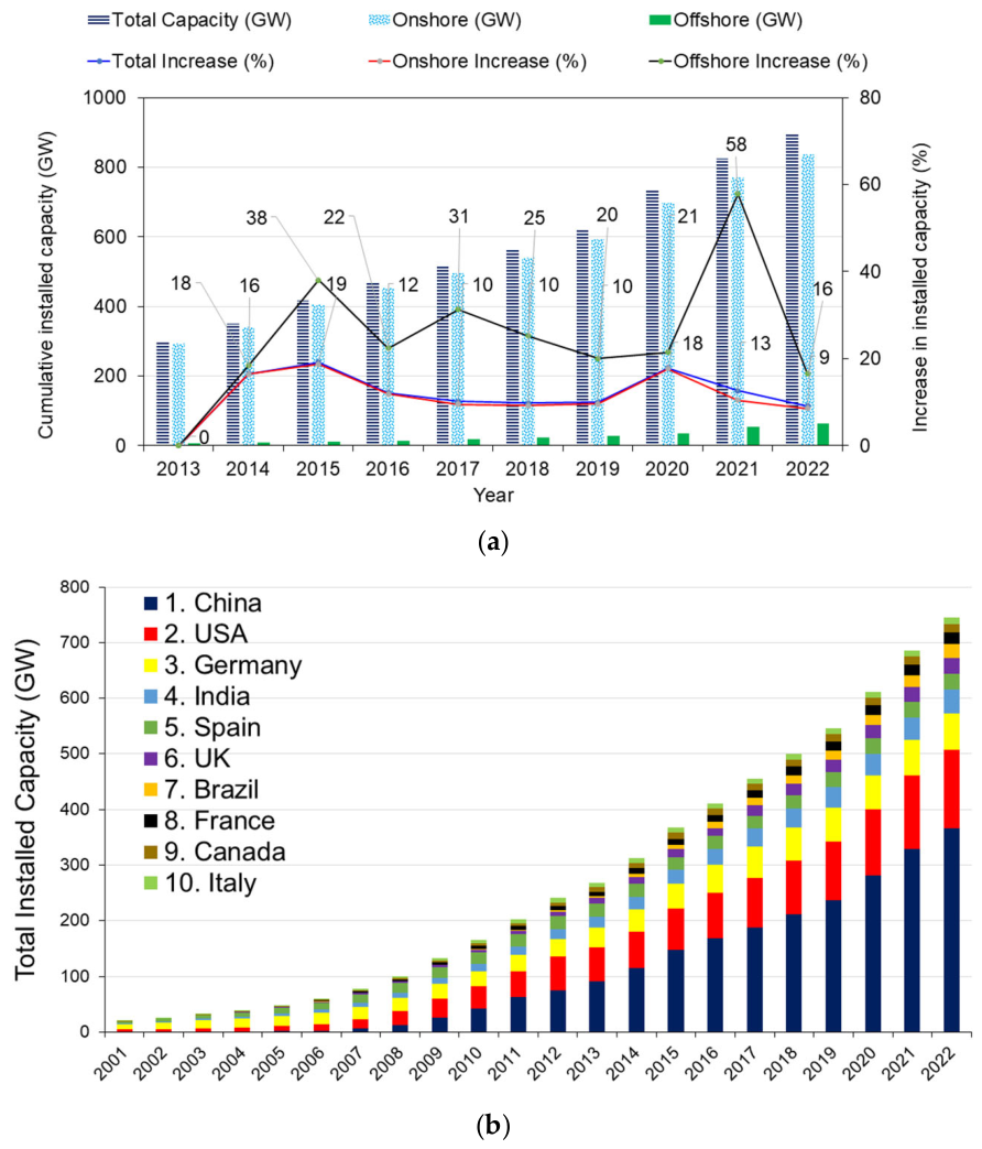
The global wind energy market is steadily increasing, with an annual growth rate of 15%, and is expected to reach an ambitious contribution of 2 TW by 2030 from a total installed capacity of 1320 GW in 2025 [11,12,13]. The projected capacity enhancements during 2020–2025 illustrate significant growth from 86 GW (2022), 121 GW (2023), 120 GW (2024), to 150 GW (2025). By 2027, a total of 60 GW of onshore wind capacity is expected to be added in North America, 26.5 GW in Latin America, and 17 GW in Africa and the Middle East. It is important to note that the apparent market share of the developing countries in terms of total installed capacity has improved significantly over the past two decades, as China, the USA, Germany, India and Brazil form the top five nations as of 2025 (Figure 1). A direct reflection of the deceptive developments in energy investment as well as international energy trade policies can be observed in the increasing number of wind farms being established with leading turbine manufacturers across the globe (Tables S1 and S2).

1.2. Wind Energy Exploration in the Indian Scenario

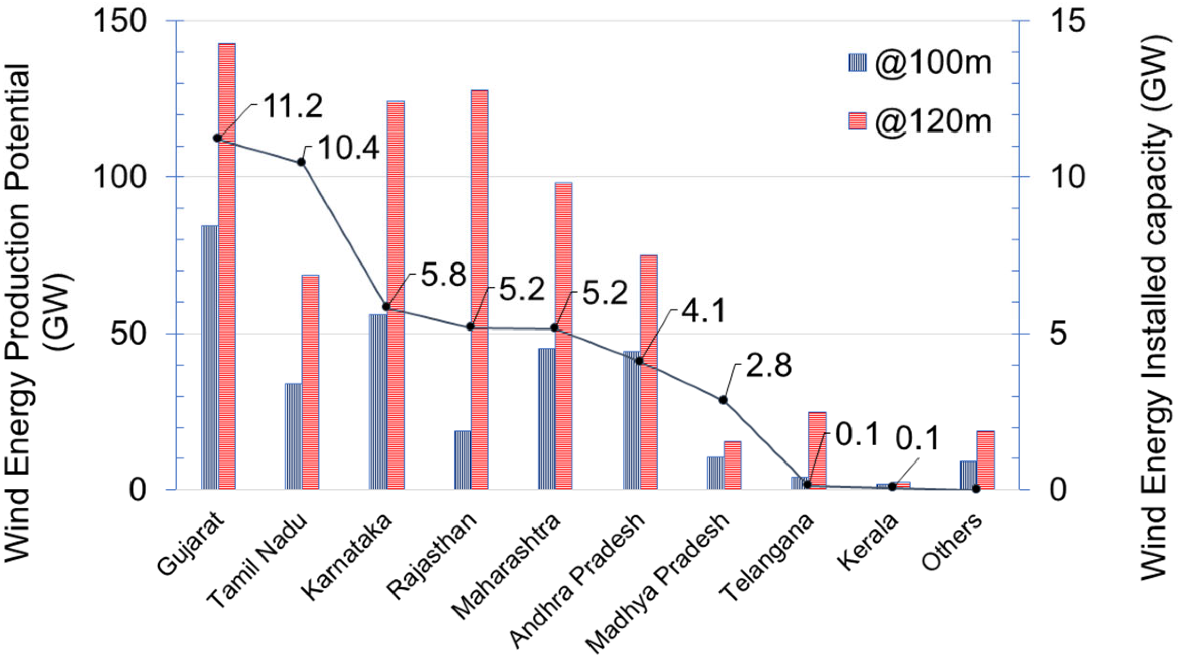
India reached the highest-ever renewable energy share in electricity generation in 2025. The non-fossil energy sources (excluding large-scale hydroelectric projects) currently account for 46.87% (236.71 GW) of India’s overall installed power capacity of 505.01 GW, of which wind energy holds the second-largest portion (10.61%) after solar energy (25.73%) with an installed capacity of 53.6 GW (as of 31 October 2025) [14]. The government of India has assumed an ambitious target production of 500 GW of renewable energy by 2030, of which 140 GW is expected from wind energy. However, out of the 28 administrative states and eight union territories in India, only seven states have significantly contributed so far to wind energy production (Figure 2). In terms of installed capacity, Gujarat and Tamil Nadu are the leading states, while Karnataka, Rajasthan, Maharashtra and Andhra Pradesh indicate substantial production potential, at least 50 GW each, thus making them ideal for further explorations (Table S3). Based on the estimates by the National Institute of Wind Energy (NIWE), the onshore wind production potential of India varies exponentially with the hub height, typically assessed as 49 GW at 50 m, 102 GW at 80 m, 302 GW at 100 m, and 695 GW at 120 m [15]. Considering the geographical diversities and the prevailing climatic attributes, it is not surprising to see that the exploration of onshore wind energy to reach the target production scale requires considerable upscaling of existing wind farms.

The moderated wind profile circulating over peninsular India shows nearly 35% of the annual mean wind speed falls under class 7 (poor), with an average wind speed record of about 2.8 ± 0.7 km/h. Only Gujarat and south Tamil Nadu have reported a consistent average annual wind speed greater than 15 km/h, while some parts of Karnataka, Andhra Pradesh, Maharashtra, Madhya Pradesh and Rajasthan achieve an average wind speed of 10–15 km/h [16]. As the expansion of the Indian wind market is at a rapid rate, with more avenues open for global investments and indigenous technology developments, a reliable estimate of the apparent wind energy production potential based on the wind speed distribution (WSD) is crucial in this regard.

Several challenges exist in exploring the medium- and micro-scale wind energy potentials of India. From a technical perspective, the available data may not be sufficient to conclusively explore the possibilities of promoting large-scale wind energy projects for other states owing to their typical climatological and economic conditions. This scenario highlights the necessity for a comprehensive analysis to predict the wind energy potential across India, aiming to identify both opportunities and commonalities that can lead to a unified rating system for wind energy producers. These estimates are typically based on statistical predictions on account of the projected frequency distribution attributes developed using various analytical methodologies.

1.3. Wind Energy Prediction Strategies

Most of the earlier studies were asymptotically limited to providing only a screening-type analysis using historical climate data for estimating the feasibility of establishing wind energy as an attractive alternative resource. Typically, the wind energy potential (in terms of WPD) depends on the prevailing wind speed frequency distributions, and the corresponding probability distribution function is used to evaluate the trend of data. Among the popular models, the two-parameter and three-parameter Weibull functions are widely used as reference distributions in many wind data analysis systems. In one of the earlier studies, Akpinar and Akpinar [17] compared the feasibility of locations and turbine characteristics for Turkey based on the data collected during the period of 1998–2003. Delina et al. [18] proposed a reliable capacity factor of 0.35 for wind turbines based on seasonal climatic data for the Hong Kong islands. Jowder et al. [19] reported an exponential correlation between the average annual WPD (from 114.5 W/m² to 816.7 W/m²) with turbine height (10 m to 60 m) for the Kingdom of Bahrain based on hourly wind speed data during 2003–2005.

Recent studies focus more on optimizing the infrastructure for harvesting wind energy at identified locations, as well as proposing newer locations and heights for enhancing productivity and sustainable operation. For example, Gao et al. [20] provided a techno-economic feasibility study confirming and validating the proposed offshore wind energy projects for Australia. Apart from the technical design aspects, financial security, fair supply-chain market and political will are summarized as the key factors for encouraging wind energy projects in developing countries [21]. On a closer look, the social acceptance factor is not sufficiently addressed in most of the earlier studies owing to a lack of convincing evidence based on realistic estimations of economic benefits and sustainable outcomes [22]. In fact, the existing operational conditions largely comprise suboptimal results even in developed countries. Therefore, it is critical to obtain a comprehensive view, from understanding wind flow patterns to the operational strategies of wind farms.

For the Indian scenario, however, only a few studies have been conducted at the regional level addressing local needs, based on a limited database. Researchers have studied the wind energy potential of Tamil Nadu, one of the windiest states in India, using various datasets over different periods [23]. Rehman et al. [24] assessed the wind energy potential of three sites located at different elevations (Chennai, Coimbatore and Erode) based on data collected from 1980 to 2017. The average power density along the coastal regions of Tamil Nadu ranges from 208.6 W/m² to 684.2 W/m² as reported by Boopathi et al. [25]. Chandel et al. [26] determined the WPD from the cumulative wind distributions by evaluating suitable Weibull parameters for 12 locations in the western Himalayan region of India using data collected between 2008 and 2012.

In the Indian scenario, most of the research works focus only on the identification and selection of suitable distribution models for wind predictions [27,28]. In a recent study, Sakuru and Ramana [29] identified the region-wise abundance of wind resources in the mainland of India using the Weibull distribution model with the help of remote sensing data collected over four decades. They suggested that land use modifications can help improve the harnessing of wind energy from sparsely vegetated areas. In this context, it is imperative to determine whether many locations in the country have a sufficiently strong wind profile but fail to report it due to insufficient measurement coverage. The latest wind energy assessment reports [1,2] substantiate this fact by stating that the cumulative national potential can become more than what is estimated so far by considering the scope of exploration.

Despite attempts to balance the continuously increasing energy demand with sustainable development goals, significant techno-economic challenges still hinder the rapid deployment and utilization of renewable energy resources and the establishment of reliable, clean, and sustainable energy production systems. One major technical issue is the variability of vertical wind speed profiles, which directly affects the selection of turbine hub height and turbine capacity. This challenge can be partially addressed by developing appropriate discrete-distribution models and using reliable large-scale datasets to evaluate wind speed distributions at different heights more accurately. Secondly, there is a global market-associated financial risk in the project investment, management and operational aspects, which necessitates measures to ensure debt service coverage and other risk mitigation plans. This necessitates the formulation of a comprehensive wind power rating system based on the operational parameters, such as capacity utilization and the effectiveness in energy transition, aimed at longer periods of operation. Many earlier studies address either the potential of harnessing or the stand-alone economic feasibility of renewable energy projects; however, a comprehensive wind power rating system for the prioritization of potential sites across the states of India has yet to be explored.

Several studies report the complexities of Indian wind systems, but in localized purviews for the purpose of simulation, with arguably “unifying distribution models.” The myriad of WPD estimates available in the literature, therefore, severely lacks comparability and compatibility for further analysis. Based on these remarks, the present study aims to evaluate the WPD for selected locations throughout the Indian states based on their topographic features and techno-economic operational parameters. Based on the estimated wind power potential and economic factors, a comprehensive rating method is formulated for prioritizing the potential sites and comparing their feasibility for future explorations. The novelty lies in the development of a framework that combines the evaluation of advanced probability distribution functions beyond conventional models, such as the Weibull distribution, with rating and variability indices to improve the accuracy and site-specific assessment of wind energy potential. This study is the first of its kind to provide the most extensive data on wind power calculations for the country, based on recorded wind speed data from 87 locations over 43 years.

2. Materials and Methods

2.1. Description of the Study Area

The study area comprises the peninsular Indian subcontinent, considering 28 administrative states and 8 union territories covering the entire landscape of geographical distributions. As evident from the previous section, the most preferred regions (in terms of capacity utilization factor, CUF) are located in the coastal border states, especially Gujarat, Tamil Nadu, Karnataka, Maharashtra and Andhra Pradesh, while there are pockets of scattered wind power potential in Kerala, Madhya Pradesh, Telangana, Jammu & Kashmir, and Rajasthan. It has also been observed from the reports of the NIWE that there are locations of moderate wind power potential in the states of Punjab, Haryana, Uttarakhand, Bihar, West Bengal, Odisha and the Northeastern States. In addition, there may be a few pockets of recirculating air flows in many parts of the country where the wind is strong due to local effects, but this cannot be captured in the report due to the absence of absolute measurements.

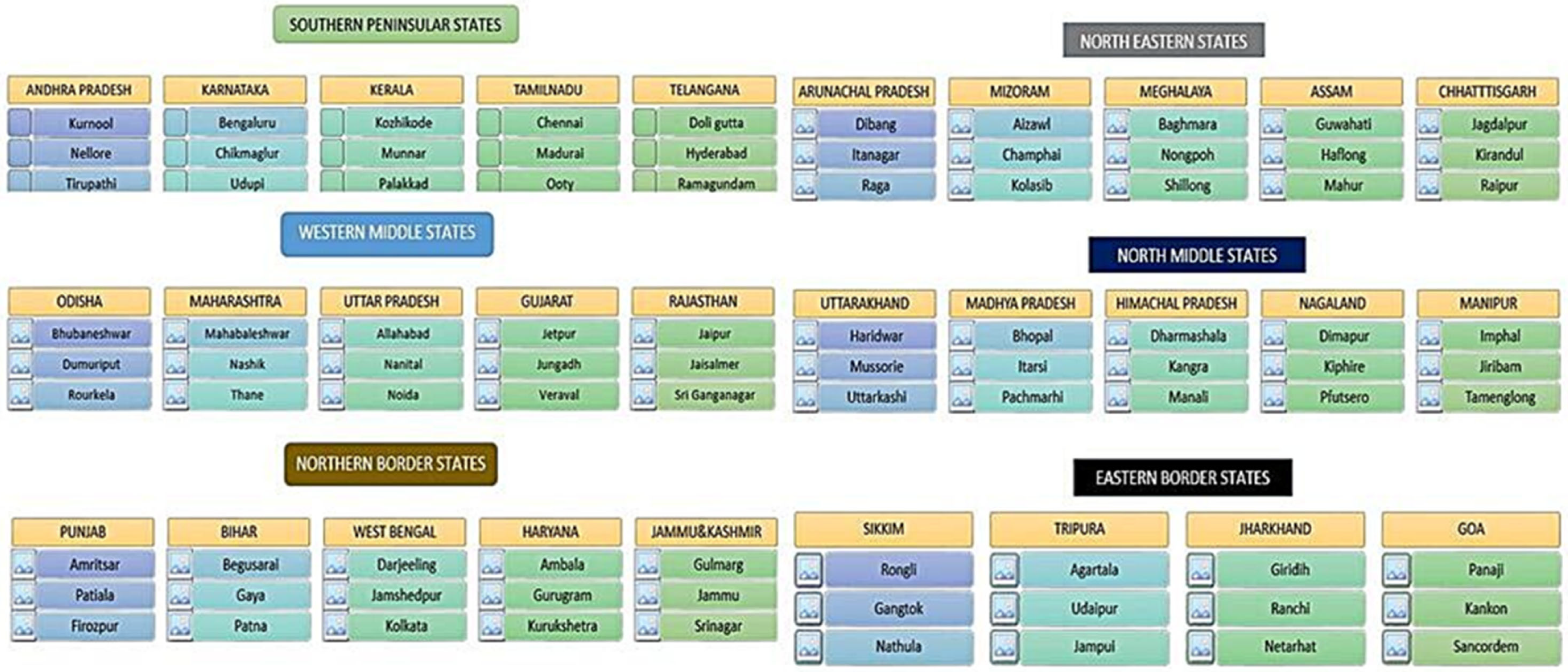
For the purpose of data collection and analysis, we have divided the country into six regions, namely the Southern Peninsular States (SPSs), Western Middle States (WMSs), Northern Border States (NBSs), Northeastern States (NESs), North Middle States (NMSs), and Eastern Border States (EBSs). Each of the regions contains 4–5 states taken together based on the similarity in their wind speed profiles, in addition to the local climatic and geographical conditions. Three unique locations were chosen from each of the states to estimate the wind energy production potential based on altitude, defined as low, medium and high. The rationale for choosing these locations may be attributed to the available records pertaining to the local climatic and geographical conditions. More specifically, the exact locations for the present study sites were chosen by considering the (i) terrain elevation features (representing low, medium, and high within the state’s average elevation ranges), (ii) land use/development features (avoiding unsuitable sites such as urbanized plots, reserved forests, etc., and prioritizing developing regions with direct accessibility and land leasing potential), and (iii) interpolated wind speed values (showing consistent records of significant deviation between low and high flow patterns). Though we have not employed analytical models for site selection, the suitability of a location is attributed to the cognitive interpretation, verifying whether it satisfies the above three conditions or not. In addition, some of the union territories are excluded from the study due to various administrative and security reasons of national interest. A summary of the study area and locations is represented in Figure 3.

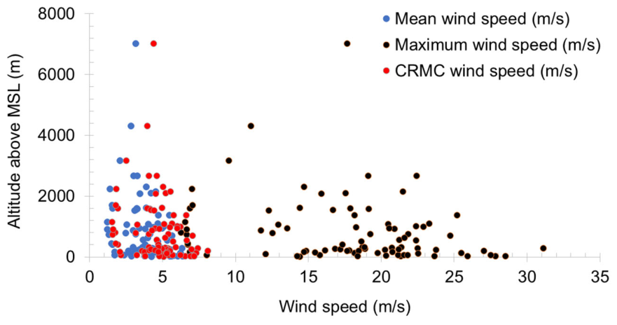
Among the classified regions, at least 10 locations are at an altitude greater than 2000 m above mean sea level (MSL), the top three highest locations being Mussoorie in Uttarakhand (which comes under the NMSs), Nathula in Sikkim (which comes under the EBSs), and Dibang in Arunachal Pradesh (NESs). The lowest locations are identified to be along the coastal belt of India, the lowest being Kozhikode in Kerala (which comes under the SPSs), Chennai in Tamil Nadu (which also comes under the SPSs), and Veraval in Gujarat (which comes under the WMSs). Most of the other selected locations have a moderate elevation, making them accessible to the prevailing wind flows emanating from oceans, following southwest as well as northeast directions through the two major monsoon wind systems. As mentioned above, the selection of locations is indifferent to their topographic altitudes, as altitude alone does not exert a strong linear control on wind speed characteristics across the study area (Figure 4).

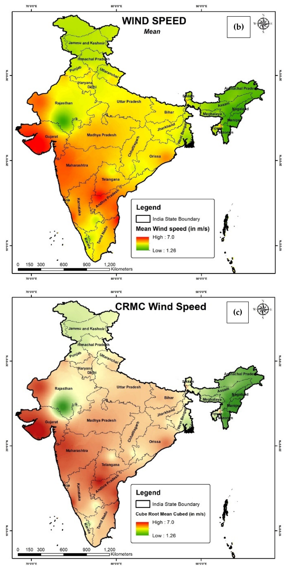
Mean wind speed values are predominantly concentrated between 2 and 6 m/s over a wide range of elevations, suggesting that local topographic features, terrain roughness, and regional atmospheric circulation patterns may influence wind behavior more strongly than elevation itself. Similarly, Cube-Root Mean Cubed (CRMC) wind speeds generally follow the trend of mean wind speeds but exhibit slightly higher values because of the greater weighting assigned to stronger wind events. The close clustering of mean and CRMC wind speeds indicates that most locations experience relatively stable wind regimes without frequent extreme wind occurrences. This may be attributed to the fact that the diversification of wind flow patterns over different terrains has dissipated the initial energy, resulting in an undulating wind profile across the elevations. This is further subjected to localized variations owing to the spatio-temporal changes in temperature and pressure within the land regions.

In contrast, maximum wind speed displays considerably greater variability, ranging from approximately 7 to over 30 m/s across the elevation spectrum. High maximum wind speeds are observed at both low and moderate altitudes, indicating that extreme wind events are not confined to higher elevations. Several locations below 500 m MSL exhibit maximum wind speeds exceeding 20 m/s, while some high-altitude locations show only moderate maximum wind speeds. It is interesting to note that out of the selected 87 locations, about 40% of the sites have recorded a maximum wind speed value above 20 m/s, of which 60% are from the non-windy states as identified earlier (Figure 2). Hence, the present study elaborates on comparing the wind energy potential across different locations that have distinct wind flow patterns, thereby contributing towards further considerations.

The Cube-Root Mean Cubed (CRMC) wind speed is an energy-equivalent wind speed that accounts for the cubic dependence of wind power on wind speed. It is computed as the cube root of the mean of the cubed wind speed observations:

$$v_{CRMC}={\left({\displaystyle \frac{1}{n}}{\displaystyle {\sum }_{i=1}^n}{v}_i^3\right)}^3$$

(1)

where v_i represents individual wind speed measurements, and n is the total number of observations. Because wind power density varies with the cube of wind speed, CRMC provides a more realistic indicator of the wind energy resource than the arithmetic mean wind speed. Higher-wind-speed events, which contribute disproportionately to energy production, are appropriately reflected in this metric. Consequently, CRMC is widely used to characterize the energy potential of a site and to support wind energy system design and evaluation.

2.2. Data Collection and Brief Methodology

The topographical features of the selected locations are compiled by using data collected from various government agencies, ensuring that the most up-to-date and reliable data are used. The wind speed data and related parameters (direction, temperature and humidity) are extracted from satellite data provided by the ERA5 source for a period from 1980 to 2023 (43 years). The hourly distribution of wind speed data was curated and further processed to compute monthly and yearly average values. Considering the statistical distribution of the frequency data, the variability in the wind speed was analyzed using standard deviations and specific variability indices. To estimate the potential of wind for economic extraction, the WPD is computed using hourly average wind speed data. The state-of-the-art Windographer software (https://ul-renewables.com/windographer/ accessed on 21 August 2025), meant for wind data analysis, has been used for statistical analysis and wind power estimation. The wind speed index (WSI) is calculated using the percent frequency occurrences of WPD above 250 W/m². The data was checked for completeness and erroneous values using visual inspection. In our observations, the data was complete and free from errors. A value of 250 W/m² was chosen for the entire analysis, keeping in view the overall availability of the wind speed, which was 5 to 6 m/s in general. This falls under a wind power class of 2 (2− and 2+), and the corresponding WPD density lies around 250 W/m².

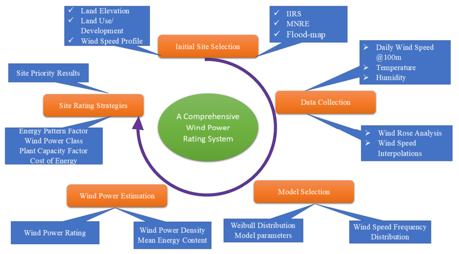
The gross wind power and annual energy yield are further evaluated using WPD values. In order to study the economic feasibility of the wind farms, the plant capacity (in terms of plant load factor, PLF and capacity utilization factor—CUF) and cost of energy (COE) are calculated based on the total investments. The critical steps involved in the analysis of wind data to achieve consensus in wind power estimation and a comprehensive wind power rating system for India are summarily presented in Figure 5.

2.3. Wind Speed Characteristics

An understanding of the variations in wind speed across time scales (diurnal, monthly, annual) is important for an accurate assessment of wind power resources. Based on the collected wind speed data, the basic characteristics of the distribution can be defined as follows.

$$\overline{V}={\displaystyle \frac{1}{N}}{\displaystyle \sum _{i=1}^N{V}_i}$$

(2)

$$\sigma =\sqrt{{\displaystyle \frac{1}{N-1}}{\displaystyle \sum _{i=1}^N{\left(V_i-\overline{V}\right)}^2}}$$

(3)

$$V_{h_2}=V_{h_1}{\left({\displaystyle \frac{h_2}{h_1}}\right)}^{\alpha }$$

(4)

where $\overline{V}$ is the average wind speed (m/s), σ is the standard deviation, V_h1 and V_h2 are the wind speeds at h₁ and h₂ heights (m), α is the wind shear exponent, and N is the number of data points. In the present case, a value of 0.14 is assigned for α [7].

The WPD is defined as the power availability per unit rotor swept area and is independent of the turbine specifications, as given below:

$$WPD={\displaystyle \frac{1}{2}}\rho {\overline{V}}^3$$

(5)

where WPD is the wind power density (W/m²), and ρ is the air density (kg/m³).

2.4. Statistical Distribution Analysis

The Weibull probability distribution model is considered in this study to analyze the variability of wind speed data over the study period. The Weibull distribution was selected because of its demonstrated capability to accurately represent wind speed frequency distributions while maintaining computational simplicity and parameter interpretability. Compared with alternative models, such as the Rayleigh, lognormal, and gamma distributions, the Weibull model offers greater flexibility through its shape and scale parameters, allowing it to capture a wide range of wind regimes.

$$P(V)={\displaystyle \frac{k}{A}}{\left({\displaystyle \frac{V}{A}}\right)}^{k-1}{e}^{\left[{\left(\frac{-V}{A}\right)}^k\right]}$$

(6)

where k and A are the shape and scale factors of the Weibull model, respectively. These parameters can be determined by using the following approximations.

$$k={\left({\displaystyle \frac{\sigma }{\overline{V}}}\right)}^{-1.086}$$

(7)

$$A={\displaystyle \frac{\overline{V}}{\mathsf{\Gamma }\left(1+\raisebox{1ex}{$1$}\!\left/ \!\raisebox{-1ex}{$k$}\right.\right)}}$$

(8)

where Γ is the gamma function, which can be defined by the following integral:

$$\mathsf{\Gamma }(V)={\displaystyle {\displaystyle \underset{-\infty }{\overset{\infty }{\int }}}{t}^{V-1}{e}^{t}dt}$$

(9)

The average wind speed and WPD values obtained from Equations (1) and (4) are considered to find the best-fit distribution by estimating Weibull parameters A and K using Equations (6)–(8).

2.5. Determination of Wind Variability Indices

The existence of extremities in the wind energy production values across the monthly frequencies is evaluated using the monthly wind variability index (MWVI), as suggested by Gonçalves et al. [30].

$$MWVI={\displaystyle \frac{WP{D}_{MEM}-WP{D}_{LEM}}{WP{D}_{MEP}}}$$

(10)

where WPD_MEM, WPD_LEM, and WPD_MEP are the wind power densities for the most energetic months (June and February), the least energetic months (January, November and December), and the mean over the entire period of data collection (1980 to 2023), respectively. Lower values of these indices represent reduced wind turbulence and hence indicate uninterrupted service life of wind turbines.

Similarly, the annual wind variability index (AWVI) is calculated using the following equation:

$$AWVI={\displaystyle \frac{WP{D}_{MEY}-WP{D}_{LEY}}{WP{D}_{MEP}}}$$

(11)

where WPD_MEY, WPD_LEY, and WPD_MEP are the WPDs for the most energetic years, the least energetic years, and the mean over the entire period of data collection, respectively. For the present dataset, between 1980 and 2023, the years 2000 and 2003 were the most energetic years, whereas the years 1997, 2014 and 2019 were the least energetic years.

The consistency of WPD above a certain magnitude is important for continuous power production at a site. As mentioned by El Khchine et al. [31], exploitation of wind power is reliable if WPD is above 200 W/m². Based on this consideration, an index called the WSI is defined to determine the percent frequency of occurrences of WPD above a certain target value. Considering the local meteorological conditions, the target of WPD is taken as 250 W/m² for the present study. The WSI is calculated using the following equation (Kamranzad et al. [32]):

$$WSI={\displaystyle \frac{WP{D}_{MEP}F}{MWVI}}$$

(12)

where F is the percent frequency of WPD occurrences above a fixed value (i.e., 200 W/m²) over the entire data collection period at each site.

2.6. Wind Energy and Cost Estimation

The wind power produced by a wind turbine and the annual energy yield are calculated as follows:

$$WP=WPD\times A$$

(13)

$$AEY=WP\times 8760$$

(14)

where WP and AEY are the gross wind power (kWh) and annual energy yield (kWh/y), A is the wind turbine rotor swept area (m²), and 8760 is the conversion for the number of hours in a year [33]. The efficiency of energy utilization by the wind farm is defined by the PCF, which can be calculated as follows:

$$PCF={\displaystyle \frac{AEY}{IPC\times 8760}}$$

(15)

where IPC is the installed plant capacity (kWh).

In order to evaluate the financial efficiency of the wind farm during the operation period, the corresponding COE in currency/kWh is calculated using the following formula:

$$COE={\displaystyle \frac{PIC}{AEY}}$$

(16)

where PIC is the plant investment cost (currency). The total investment cost includes the capital, installation, civil work, engineering, management, operation, maintenance, etc.

3. Results and Discussion

3.1. Scale-Dependent Variability Trends of Wind Speed

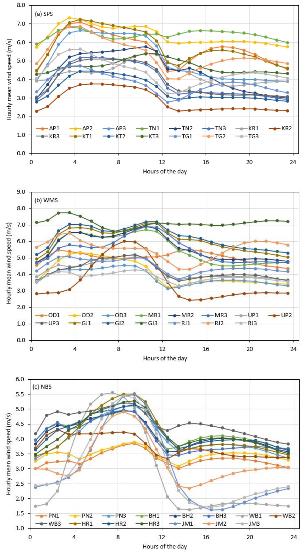
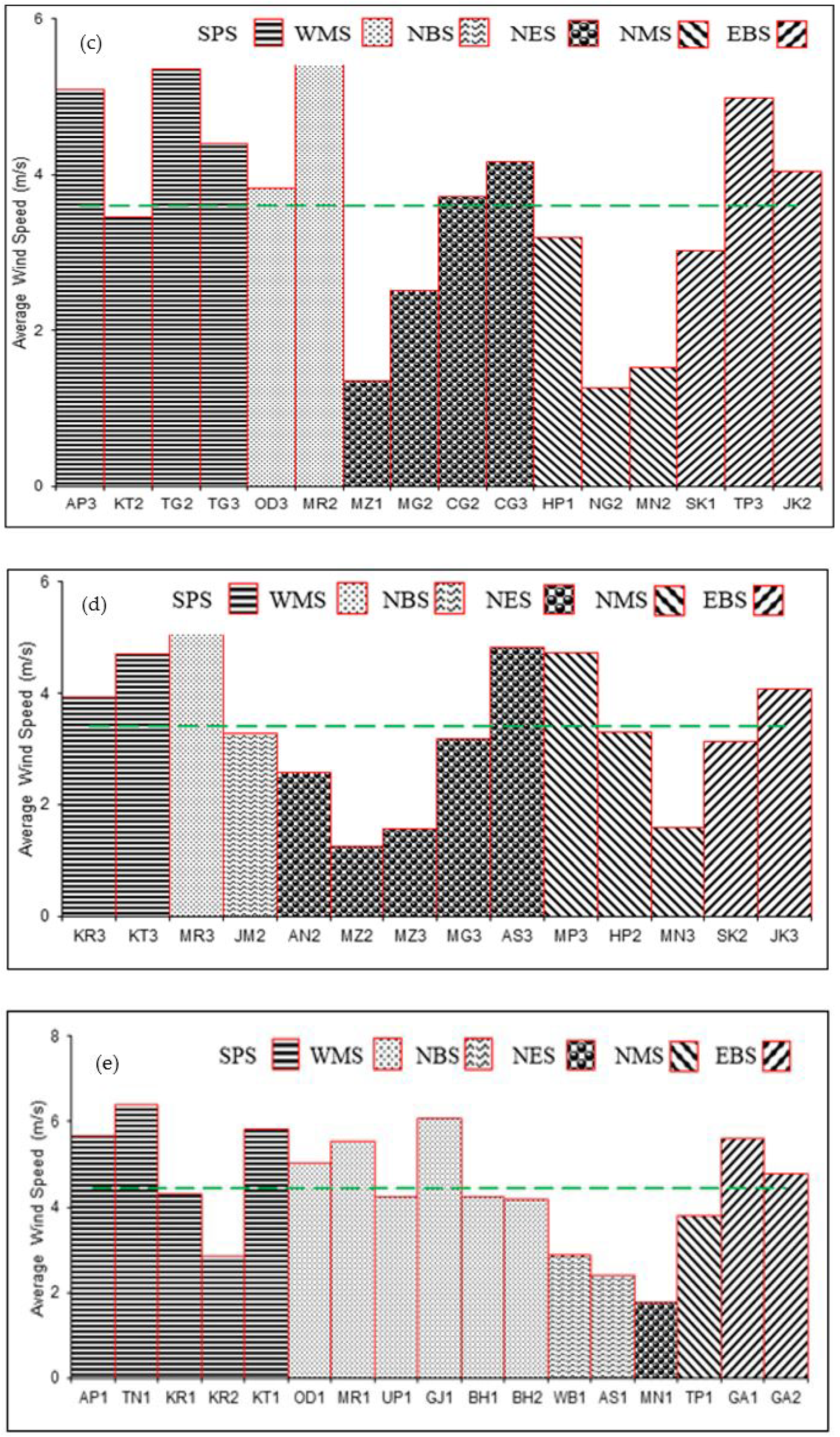
The temporal averaging of the hourly wind speed data for the selected six regions was compared for their dependency on various time scales. At the smallest scale, the diurnal variations indicate considerable deflections in the forenoon hours compared to the afternoon and night periods across all six regions of India. The periodic and orthogonal occurrence of southwest and northeast monsoons crossing the coastal boundary has significant effects on the onshore moisture flux and the precipitation pattern in the eastern and western states. Among the Southern Peninsular States (SPSs), Andhra Pradesh and Tamil Nadu have shown the highest wind speed with a minimum variation throughout the day, while Kerala and Telangana have the lowest wind profile except in the afternoon hours (Figure 6a). Further, the sea breeze circulation on the western coastal regions has higher variability compared to the eastern coastal regions, thereby exhibiting diurnal variations between the forenoon and afternoon sessions (with a difference of 1.2–2.5 m/s) in the western coastal locations.

As far as the high-altitude locations in these states are concerned, the diurnal variations are more profound and show bimodal distribution, with peaks in the early morning and evening hours (Figure S4). This is particularly distinct for the windward and leeward sides of the Western Ghats due to the influence of sea–land breezes and localized heat fluxes, while the hilly locations in the interior of the Deccan plateau experience highly variant and lesser irregular wind patterns during most of the monsoon reversals. This is in combination with the observation that peninsular Indian states receive a large number of turbulent winds from oceans that are redirected by the mountainous belts, resulting in irreducible heterogeneity in the subsequent flow patterns [34]. Being the most productive zone in the country, the wind energy farms operating in the SPSs are, by and large, favored by the monsoon patterns.

Considering the diurnal wind flow pattern in the WMSs, higher wind speeds were recorded in Gujarat and Maharashtra in the summer seasons, with bimodal peaks occurring in the mid-noon hours (Figure 6b). Being the top-rated wind-producing states in India, both these states have sufficiently stable diurnal wind profiles, irrespective of the altitudes for the selected locations. It is understood that the speed of wind at an altitude of 100 m from the surface will have an accelerating effect caused by surface heating during the daytime, while the turbulence present in the higher altitudes transfers sufficient momentum to the flow at lower altitudes during the nighttime [35]. Therefore, Rajasthan and Odisha experienced similar diurnal variations with lower velocity distributions, although subjected to two different climatic conditions. The middle-altitude location in the state of Uttar Pradesh has shown a single-peaked normal distribution trend, which was typical for the selected day of the month and is found to be quite reversible according to the seasonal climatic variations.

Among the NBS states, highly stable diurnal wind flow patterns were observed for the states of Punjab, Haryana and Bihar, where altitude variations did not make any significant difference in the average wind speed values (Figure 6c). The diurnal wind speeds showed a single-peaked normal distribution trend for Jammu & Kashmir, as well as West Bengal, where the differences for the altitudes were more significant for West Bengal, while the highest value of the statistical range was observed for the selected locations in Jammu & Kashmir (2.5–4.0 m/s). It is interesting to note that the northcentral states show significant diurnal wind flow stability, although they experience extreme climate conditions, as revealed in the seasonally averaged data. One plausible reason for this invariability in the diurnal time scale is the absence of a moderating influence from the sea, causing the vertical mixing of ground-level heat waves with turbulent winds at higher altitudes [35,36]. Nonetheless, as a small-scale phenomenon, the diurnal variations can be viewed as an intrinsic signatory proof for local atmospheric stability, giving moderately uniform wind flow throughout the days.

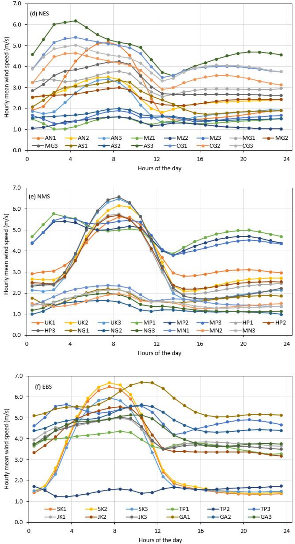
The typical hourly wind speed profiles for the NESs clearly depict unimodal peaks of wind speed during the early morning hours, followed by a drastic reduction in the afternoon hours (Figure 6d). This is primarily associated with the prevalence of orographic interference over the convectional air currents. Most of the NESs have highly undulating topography, creating a mountain–valley wind circulation pattern over the local surface-layered convection. It is notable that the average rainfall is quite heavy in the NESs (about 2000 mm annually), which are mostly concentrated on the monsoon winds [37]. It is observed that Assam, Meghalaya and Arunachal Pradesh have the highest wind speed with unimodal peaks during the forenoon hours, while the afternoon and night flows are fairly uniform without any considerable variations. The highest average wind speed (6.2 m/s) was noted for the high-altitude location of Assam (Mahur), while the highest variability (statistical range of 3.7 m/s) was observed for the low-altitude location of Arunachal Pradesh (Itanagar). The lowest wind profile was recorded by Mizoram (maximum wind speed of 1.9 m/s), making it unfit for further wind energy exploration studies. It is interesting to note that the wind profile of Assam is similar to that of Chhattisgarh, though there are considerable differences in other climatic features.

The wind speed profiles observed for the NMS states indicate that a consistent and significant diurnal wind distribution is available for the central state of Madhya Pradesh, whereas the high-range regions, such as Uttarakhand and Himachal Pradesh, have productive wind availability only during the forenoon hours owing to the atmospheric diversions caused by several mountains in the state (Figure 6e). The Northeastern States of Manipur and Nagaland also experience a consistent diurnal wind profile, mostly unaffected by the local climate conditions, but the average wind speed is found to be quite low compared to the other states in the selected region. There is a considerable difference in the dynamic nature of wind distribution traversing through the central plateau regions compared to the Himalayan valley regions, where the latter locations experience higher atmospheric mixing effects, resulting in a more consistent wind speed profile [38]. The highest difference in diurnal wind speed was observed for high-range regions, while the lowest was observed for the Northeastern States. As we observe in this study for the first time, the wind speed characteristics of the central regions of India can be significant evidence for their exploration compared to those regions with low wind availability.

For the selected locations in the EBS region, the diurnal WSD is found to be consistent and reliable, except for the state of Sikkim, which experienced a typical unimodal distribution profile (Figure 6f). The average diurnal wind speed varied from 2.8 m/s to 5.6 m/s for the selected locations in this region, except for TP2 (Udaipur), which had a value of 1.5 m/s. Similarly, the highest difference in wind speed is observed for the state of Sikkim, while Tripura has the lowest difference. It is interesting to note that a comparable wind stabilization pattern exists in the selected locations in the state of Jharkhand, similar to the coastal regions, giving evidence for the scope of exploration of wind energy production in the state. Based on the above observations, one can interpret that the diurnal variations in the wind speed can provide a good insight for the expected strategies for wind energy exploration attempts at a suitable scale.

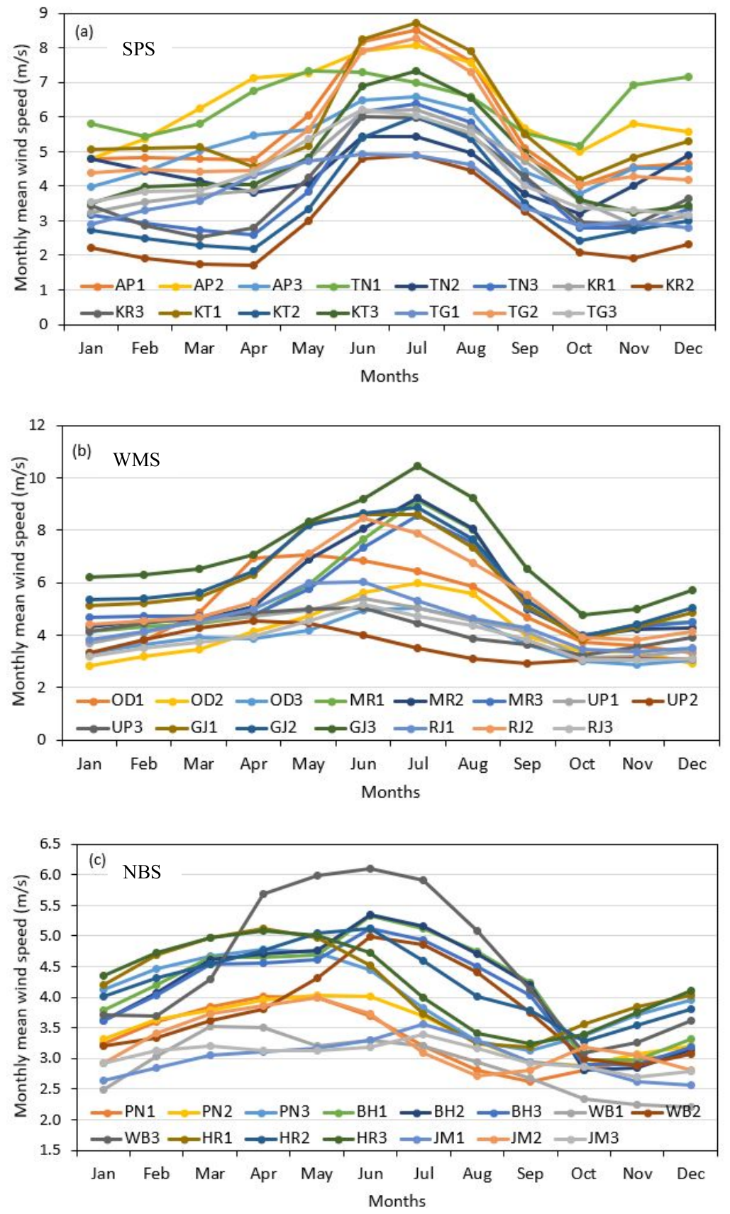
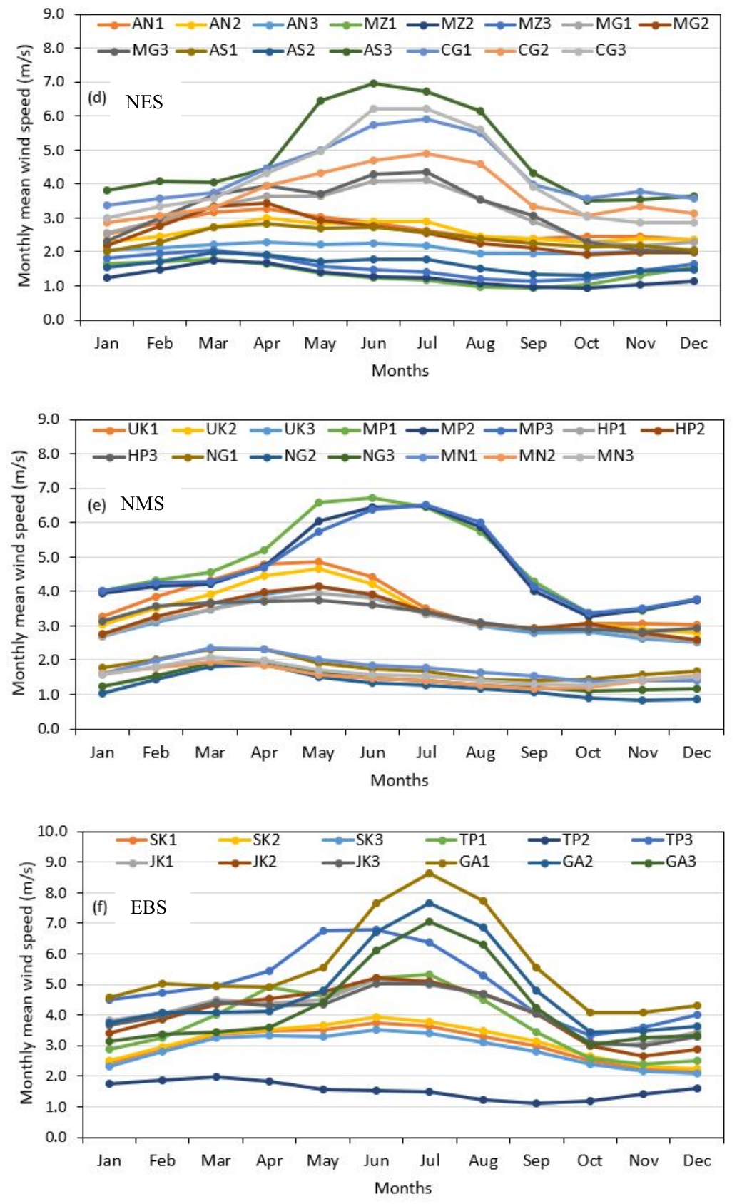
In order to differentiate the impact of temporal scaling in this context, the average monthly and average yearly wind speed profiles were compared among the six selected regions. It is observed that the effect of averaging has a significant smoothing effect on the wind speed profiles while expressing the distributions at larger scales. The monthly average wind speed profiles invariably show considerable wind flow during the monsoon months from June to August, especially for the locations with comparatively high diurnal wind speed values. Among the SPS states, an average monthly wind speed above 5 m/s is consistently observed for Tamil Nadu and Andhra Pradesh for all three levels of locations (Figure 7a). The early onset trends of the southwest monsoon in the states of Kerala and Karnataka are found to be associated with heavy winds compared to other months [28,35]. In other words, the effect of seasonal variations in the wind speed is more profoundly visible in the coastal states of India compared to the middle lands, as well as the upland hilly regions.

The average monthly wind speed for the WMS region has shown a distinct profile compared to the SPS region based on the availability of high-speed winds during the months of June–August (Figure 7b). Except for the locations in the states of Rajasthan and Uttar Pradesh, all other locations have considerable variability in their wind flow patterns, with a maximum speed (8.5 to 10.5 m/s) during July compared to a minimum speed (2.8 to 4.8 m/s) during October. Therefore, the monthly averaged wind speed data provides quite consistent estimates of the expected variations in the wind speed and their levels of significance in the context of wind energy production strategies.

The monthly variation in the wind speed profiles for NBSs and NESs showed similar distribution characteristics, with a typical peak speed season during the months of April to August (Figure 7c,d). A transition of the peak windy month is observed from April (for Punjab and Haryana) to June (Bihar and West Bengal). As observed in the diurnal variations, the lowest average wind speed values were observed for the states of Punjab and Jammu & Kashmir. The monthly profiles of Bihar and West Bengal are quite impressive, suggesting the availability of consistent and high winds throughout the seasons of the year. The average monthly wind speed values for the NES region showed seasonal fluctuations only for the locations in the states of Chhattisgarh and Assam, while all other locations experienced a uniform but low wind distribution pattern. The windiest months for these regions are expected to vary between April and July owing to the influence of other climatic variables. In comparison, the availability of a reliable wind flow is limited to those states with a modal distribution, which should be explored for utilization at suitable scales.

Based on the mean monthly wind speed variation for the selected locations in the NMS and EBS regions, several distinct profiles can be obtained, similar to the inconsistency observed in their diurnal variations (Figure 7e,f). Among the locations in the NMS region, the highest wind speed was obtained for Madhya Pradesh, but with the modal distribution peaking during the months of May to August. Considering the consistency and significance, the locations in the states of Uttarakhand and Himachal Pradesh represent attractive wind speed profiles in the range of 3.2 to 4.8 m/s. Notably, the wind speed profiles of the locations in Nagaland and Manipur do not suggest a productive range of wind speed, though the speed was quite consistent in those regions. The comparative analysis of wind speed variations for different temporal scales performed in this study provides a clear and comprehensive picture of the nature of challenges that exist in identifying suitable locations for wind energy extraction in a sustainable way.

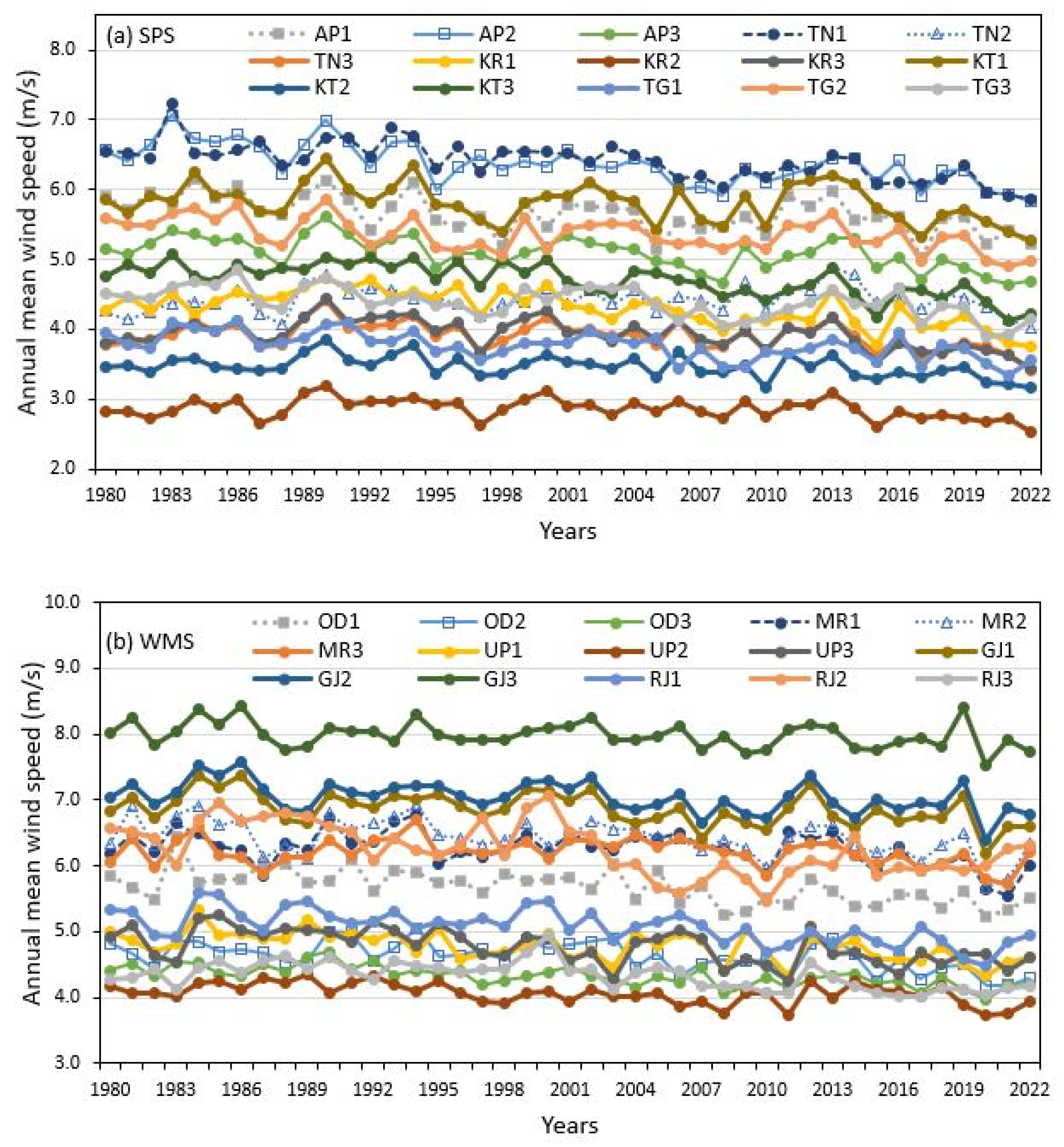
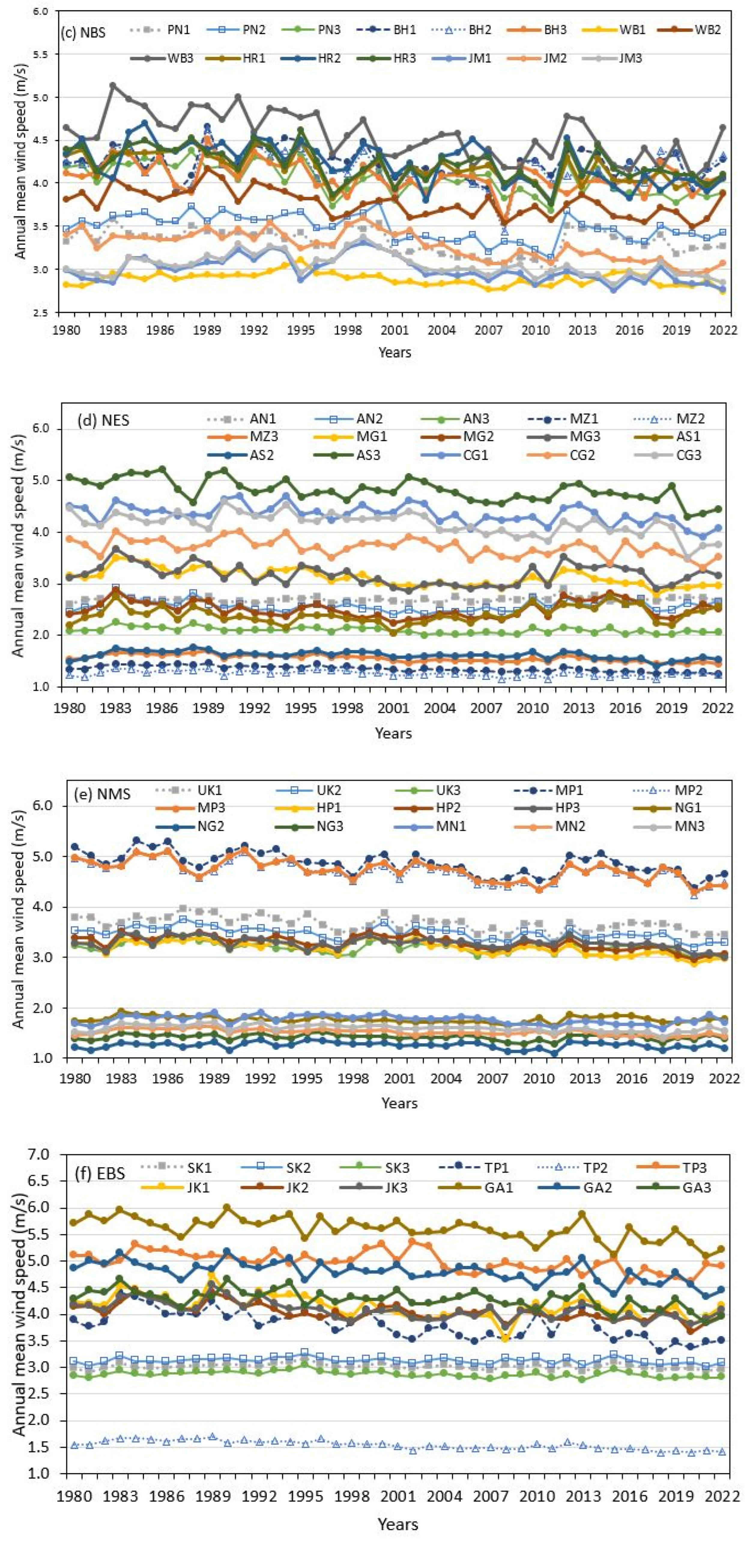
Wind speed variations based on the annual average values were compared for the selected study period in order to inspect the historical trend for change in wind speed records. It is observed that most of the states have a consistent track record of annual wind speed, with short spikes of rising and falling appearing in a few consecutive years. Apart from the hydrologic and climatic considerations, it can be safely argued that the observed wind speed profile has a seasonally repeating pattern with a short recurrence interval range (in the range of 5–10 years), resulting in a more or less similar wind flow pattern throughout the study period. However, when we analyze more specifically, there is a reducing trend for the annual average wind speed values for a few selected locations in the SPS region (Figure 8a,b). Similarly, the deviations in the average wind speed values are quite similar for most of the locations in the NBS and NES regions (Figure 8c,d).

As far as the NMS and EBS regions are concerned, the average annual wind distribution profiles are distinct and consistent for the records during the study period (Figure 8e,f). Hence, based on the comparative evaluation of wind speed profiles for different time scales, it is possible to critically propose strategies for exploring wind energy at suitable scales. Considering the acute demand for sustainable energy production and distribution for a wide range of applications, there is an immense possibility to translate these observations into suitable workable models by making them compatible with the local site’s climate and other economic factors.

3.2. Spatial Distribution of Wind Speed

The distribution of wind within the Indian peninsular region has been viewed primarily with the onset, progress and dispersion of the monsoons. Apart from this, occasional convective drifts, occluded fronts, atmospheric inversions and local heating effects contribute to the wide variety of wind speed patterns observed in lateral and vertical directions [22,23,24,25,27,28,29,36,37]. The exponential trends of wind speed variations according to the height are observed to be consistent for the selected study regions (Figure S4). The shear exponent, α, is considered to be 0.14 for the extrapolation of wind speed at higher altitudes for studying enhanced production strategies. The results are based on the projected wind speed at various demarcated vertical profiling sections, such as 10 m, 50 m, 100 m and 120 m. The WMS and NMS regions have shown a minimum increase in wind speed with respect to the height above ground up to 120 m compared to the other regions. The extrapolated values of wind speed at 120 m are quite different among the locations within a region, and this variation is more clearly visible for the regions where the temporal wind speed profiles have shown distinct ranges owing to the particular atmospheric and topographical conditions. In the absence of any unexpected situations, the availability of wind at 100 m and 120 m is considered to be the most promising for exploring wind energy in the developing locations in the study area.

Apart from the wind speed values, the direction at different heights above the terrain plays a significant role in evaluating the productive wind availability in a given location. By looking at the wind rose diagrams derived from the collected wind speed data at a height of 100 m (also done for 120 m), it is possible to ascertain the potential of the prevailing wind in order to propose a suitable direction for the erection and sustainable operation of wind farms (Figure S5). It can be inferred that the majority of the locations in the SPS and WMS regions will benefit only from western winds, with fewer contributions from other directions. Similarly, the NBS and NMS regions have shown the highest distribution of wind in multiple directions, indicating the availability of consistent wind flow without the adverse impact of seasonality. However, the NES and EBS regions are favored by the wind flows mostly coming from the south and west directions, indicating the possibility of benefiting from the availability of consistent and significant wind flow patterns.

In an attempt to evaluate the inconsistencies existing in the implicit interactions between the geographic altitude and the prevailing wind speed, an analysis of the wind speed characteristics according to different altitude zones is proposed. Based on the inferred input database and the updated history of strategies for wind power exploration, the selected locations in the six study regions are separated into groups of varying altitudes above mean sea level (MSL), namely low altitude (LA) [<100 m], medium altitude (MA) [100–500 m], high altitude (HA) [500–1000 m], very high altitude (VHA) [1000–2000 m], and extremely high altitude (EHA) [>2000 m]. It is found that out of the 87 study locations, 17 locations are under LA, 30 are under MA, 16 are under HA, 14 are under VHA and 10 are under EHA categories of altitude. It is important to note that this classification tends to overrule the previous considerations of the relative identification of three locations at the local scales (i.e., low, medium, and high) within every administrative state. It is imperative that some of the medium stations in certain states merge into the new LA category and vice versa. The purpose of this analysis is to get a more stable scenario of average WSD in various altitude classes that belong to different regional groups defined earlier.

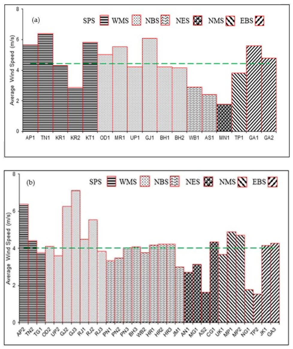
It is observed that most of the sites under the LA category belong to the SPS and WMS regions, which are mostly located on the west coast (Figure 9a,b). The average wind speed under this category is found to be 4.44 ± 1.36 m/s. In comparison to the results from the temporal-scale variations, these locations ensure significantly consistent wind flows and therefore justify harvesting strategies for future explorations. The average wind speed variations for the locations under the MA category cover the largest area of India [39]. The average wind speed under this category is 4.01 ± 1.26 m/s (Figure 9c,d). The majority of locations under this altitude class belong to the WMS (Gujarat, Rajasthan) and NBS (Punjab, Haryana) regions. The WMSs have distinct wind exploration strategies, considering the economic, social, and eco-friendly readiness of the locations.

The average wind speed among the locations under the HA category is found to be 3.59 ± 1.40 m/s, for which the majority of stations are spread in the SPS, NES and NBS regions (Figure 9e). The reason for the lower average value of wind speed at this altitude range may be attributed to the grouping of locations belonging to the NESs and NBSs, which have very poor wind profiles despite their high-altitude mountainous terrains. The average wind speed decreases to 3.40 ± 1.32 m/s when considering even higher locations in the VHA category. The main contributors in this category belong to the NES and EBS regions, where the presence of high-altitude mountains has not significantly contributed to the redistribution of consistent wind profiles. Adding further to the topographic diversity of India, the regions grouped under the EHA category have resulted in the lowest average wind speed values of 3.21 ± 0.94 m/s. The results of this analysis indicate that a mere grouping of regions on account of their similarity in altitudes does not provide sufficient linkage to the generation of consistent wind profiles at higher altitudes, counter to conventional interpretations. Based on this inference, we further investigate the validity of our hypothesis on the non-dependency of topographic altitudes on the wind power production potential.

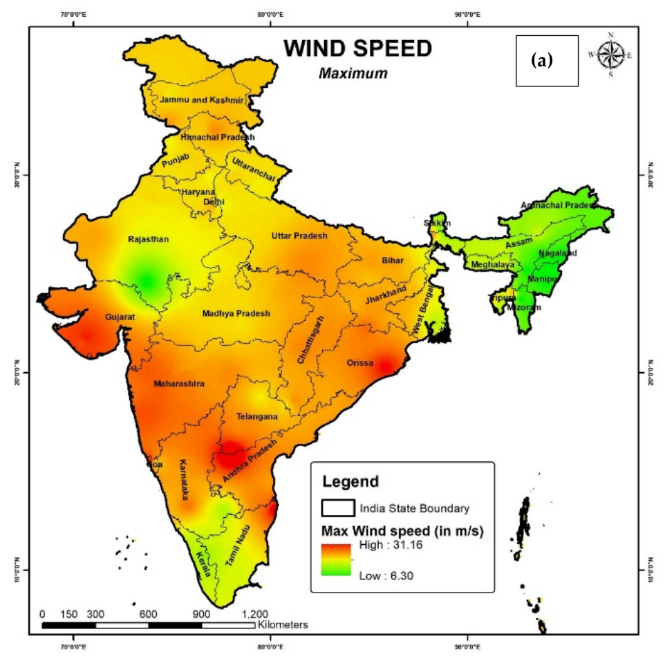
Based on the calculations of average, maximum and Cube-Root Mean Cubed (CRMC) wind speed values for the selected locations in the six regions, the distribution profiles are depicted in the Indian map (Figure 10). All three maps show similar trends, but vary in their range of obtained values (Figures S1–S3). The maps show a gradual interpolation based on the wind speed data taken from the given locations, resulting in other locations with similar opportunities for wind energy exploration. However, it must be noted that land use practices, terrain features and other unnoticed obstacles must be addressed to make it more convenient to propose wind farms. Given the available wind energy production units in the country at present, the results indicate the possibility of identifying further locations for installing wind farms, thus making this more conservative, reliable and cheap.

3.3. Spatial Distribution of Wind Power Potential

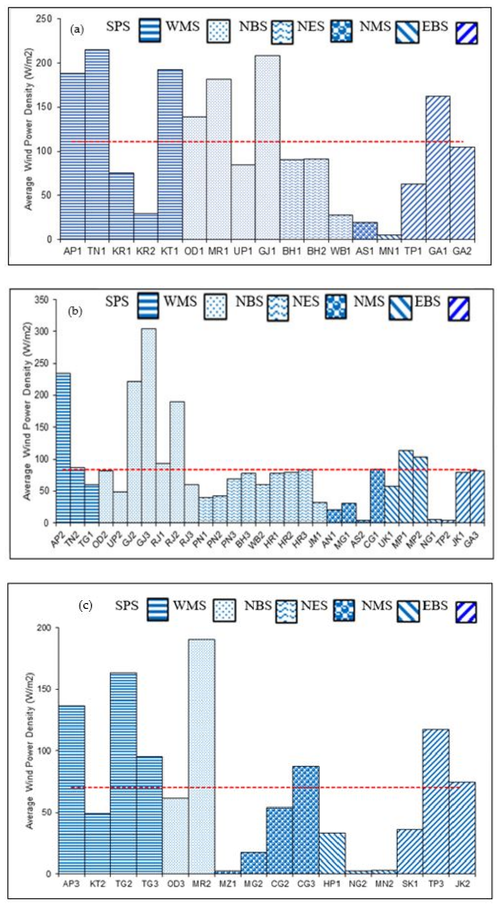
The estimation of wind power based on the cubic law indicates a direct correlation with the wind speed for the selected six regions of the country. The existing potential for exploring wind power for a selected location is typically expressed in terms of WPD and has been evaluated based on diurnal, monthly and annual wind speed profile variations, Figure 11a–e. This discussion omits the plots of the resulting trends, which closely resemble the corresponding wind speed profiles. However, this exercise was necessary to assess the possibility of temporal scale dependency on wind power potential, similar to the WSD presented in the previous sections. Although the variabilities in wind speed are quite inconsistent at lower temporal scales, one can very well appreciate the untapped potential existing in the central as well as some of the high-altitude regions of the country by deploying suitable means of extraction to cater to the growing energy demands.

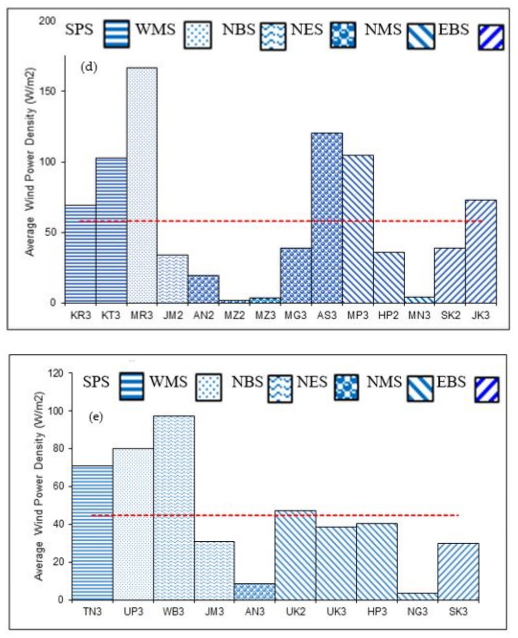
Based on the average annual WPD obtained for the selected locations, a comparison has been made here to attribute the influence of regional altitudes on the observed average values (Table S4 and Figure S6). It is observed that the highest value of the average WPD (110.6 W/m²) is for the lower altitude (LA) group, with the majority of the locations belonging to the SPS and WMS regions, Figure 11a. This average value, nonetheless, depicts the minimum wind flow condition despite the highest values of TN1 (214.7 W/m²) and GJ1 (208.4 W/m²) because of the dampening effect of poor wind-flowing locations within this group (such as Mn1, AS1 and WB1). The largest group under the elevation-based categories is MA, which has 30 locations where the average WPD is found to be quite low (84 W/m²) despite the peak values for GJ3 (304.8 W/m²), AP2 (233.7 W/m²), and GJ2 (222.1 W/m²), Figure 11b. For the HA group, the average WPD is found to be 70.2 W/m², while the high-performing locations are MR2 (190.2 W/m²) and TG2 (163.3 W/m²), see Figure 11c. On a similar note, the average values for the VHA (Figure 11d) and EHA (Figure 11e) groups are observed to be 58 W/m² and 45 W/m², owing to the large number of contributing locations from the NES and EBS regions. This comprehensive analysis supports the hypothesis that wind power potential in India is not a direct function of high-altitude locations available in any particular state but depends primarily on the characteristic wind speed profiles and the prevailing topographic features.

3.4. Reliability Analysis of Wind Power Potential Using Variability Indices

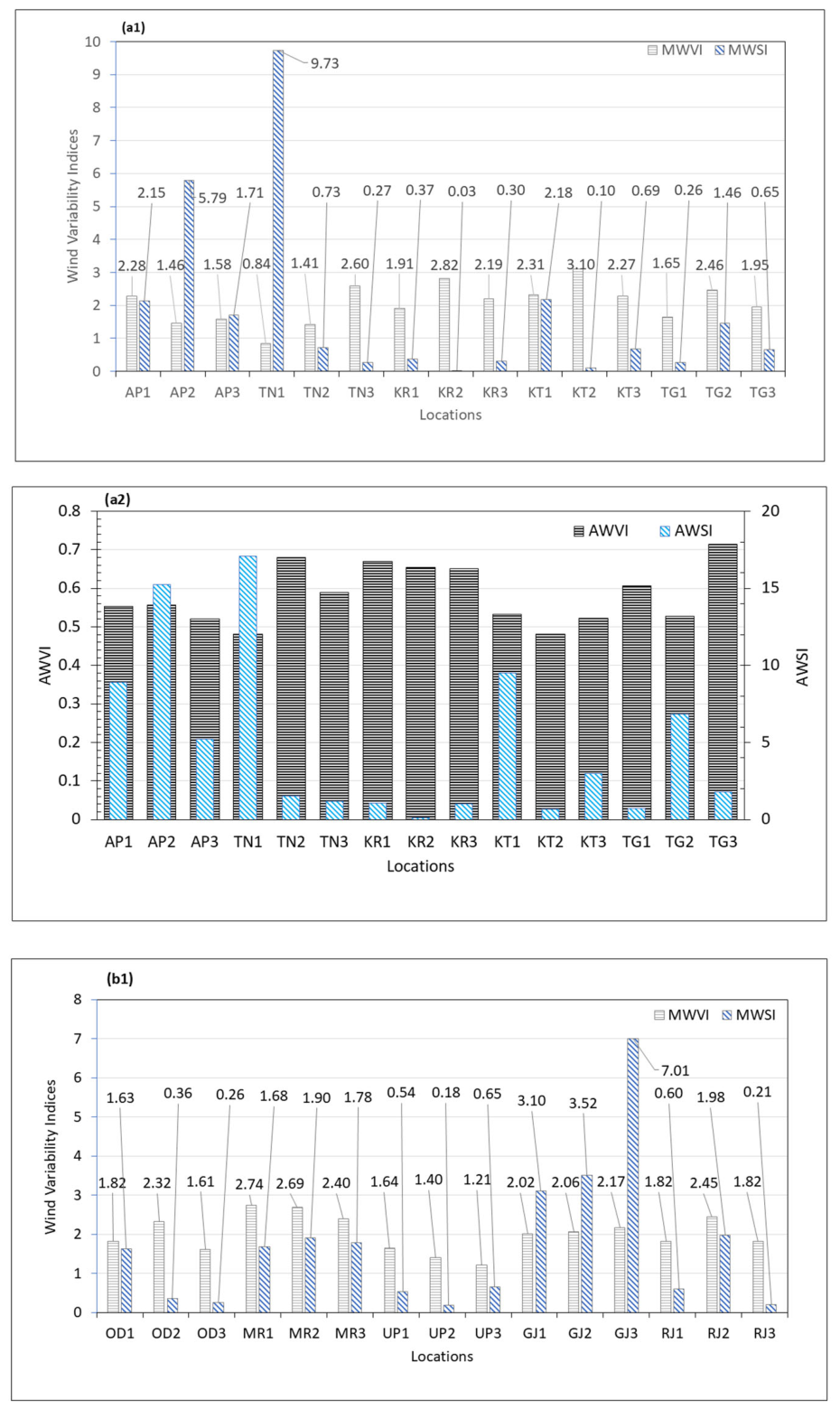
Based on the statistical distribution of the wind power potential across the selected regions, the seasonal variability in the estimated wind power values is further evaluated in terms of wind power indices. As indicated by Equations (9) and (10), the wind variability index (WVI) has a normalizing effect on the wind power distribution, whereas the WSI index makes this variability proportionate by attributing the frequency factor (percentage of occurrence of data for a set lower limit) [40]. Therefore, a comparison of WVI and WSI can ensure the reliability of the site for the expected production potential of wind, considering the effect of wind variability over the selected duration of data collection.

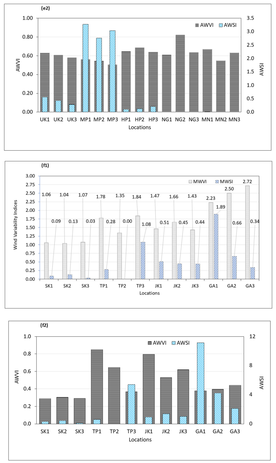
As mentioned in the previous results, the top three locations in the SPS region with the highest WPD are found to be AP2 (233.7 W/m²), TN1 (214.7 W/m²), and KT1 (192.7 W/m²). This is based on the average wind speed values observed during the selected period of data collection. The selection of top values is made under the consideration of a fixed target WPD value of 200 W/m² to compare the wind power potential throughout the country. When we evaluate the wind variability indices for all the stations, it can be observed that the highest values of the MWVI were obtained for KT2 (3.10), KR2 (2.82), and TN3 (2.60). By definition, the MWVI incorporates all possible biases originating from extremities. Therefore, this indicates the influence of extremities on the average estimated values. However, the monthly WSI values were again found to be highest for TN1 (9.73), AP2 (5.79), and KT1 (2.18), strongly supporting the influence of the frequency factor in relating to wind power potential variability, thereby indicating the reliability of sustainable exploration for a future time. The variability in terms of annual predictions indicates that the highest values of the AWVI were obtained for TG3 (0.71), TN2 (0.68), and KR1 (0.67), while the highest annual WSI (AWSI) values correspond to the same locations with the highest monthly WSI (MWSI). The results relate to the fact that a mere statistical distribution analysis can be extended for reliability estimation in order to propose the suitability of wind power potential at a certain location.

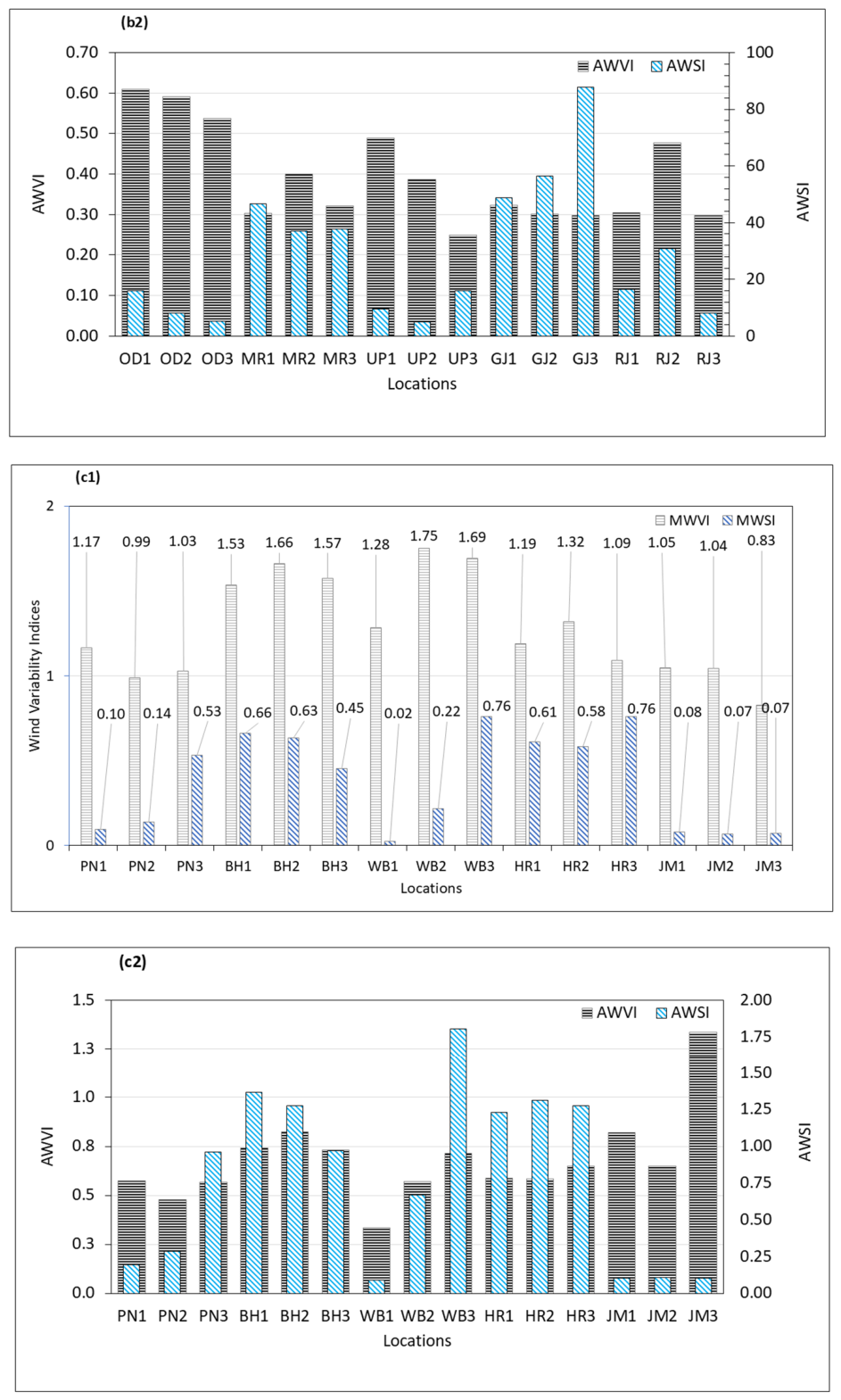
Considering the variability in WPD for the locations in the WMS region, it is observed that the highest wind power producing locations are GJ3 (304.8 W/m²), GJ2 (222.1 W/m²), and GJ1 (208.4 W/m²) while the MWVI is highest for MR1 (2.74), MR2 (2.69) and RJ2 (2.45) and AWVI is highest for OD1 (0.61), OD2 (0.59), and OD3 (0.54). The ambiguity for a stable WPD in these locations may be correlated with the typical climatic extremities, in addition to the wind speed variations. The highest values of WSI (in terms of MWSI and AWSI) are unanimously attributed to GJ1 (3.10 and 48.87), GJ2 (3.52 and 56.57), and GJ3 (7.01 and 87.87). It is also observed that the WSI of Maharashtra is higher than that of Rajasthan, while only a few other locations have significant AWSI values, such as OD1 (15.92) and UP3 (15.97).

A comparison of the wind variability indices for the locations in the NBS region revealed that the highest WSI is closely related to the highest WPD potential, although some differences exist for a few stations. The top three locations based on WPD are WB3 (97.3 W/m²), BH2 (91.6 W/m²), and BH1 (90.6 W/m²), while the highest values of MWSI are observed for WB3 (0.76), HR3 (0.76), and BH1 (0.66), and the highest values of AWSI are noted for WB3 (1.80), BH1 (1.37), and HR2 (1.31). The MWVI is highest for WB2 (1.75), WB3 (1.69), and BH2 (1.66), while the highest values for AWVI are observed for JM3 (1.34), JM1 (0.82), and BH2 (0.82). A quick analysis of the results indicates that the stability of WPD is the essential feature for qualifying to be identified, as per the WSI values, in contrast to the WVI values. It is important to understand that the numerical values of the WSI decrease significantly, even more so than the reduction in WPD across the regions.

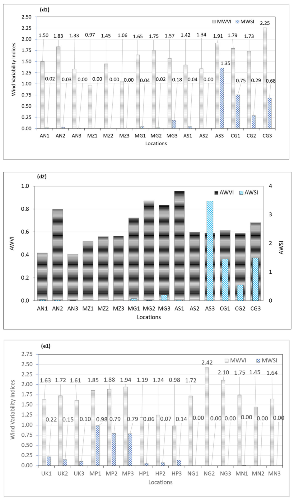
The observed trends in the variability of wind profiles among the NES region revealed that the top three locations with the highest AWSI values are AS3 (3.47), CG3 (1.49), and CG1 (1.46); the MWSI values are highest for AS3 (1.35), CG1 (0.75), and CG3 (0.68). It is important to note that most of the other states could not produce any reasonable stability profile for the WPD due to the poor or negligible frequency of the occurrence of opportunities that sufficiently match the target value WPD value of 200 W/m². This finding is in accordance with the poor values of WPD, as well as wind speed, recorded in these locations [38,39,40]. The top three values of WPD for this region are AS3 (120.7 W/m²), CG3 (87.1 W/m²), and CG1 (84.1 W/m²). However, these values are quite low compared to those of the other regions, such as the SPSs and WMSs. Based on the point of potentiality analysis, these results can be critical in selecting suitable locations for wind power exploration. In other words, the variability indices are quite indicative of the possibility of more suitable, unknown locations.

In order to evaluate the suitability of wind power production from the middle states of India, the wind variability indices for the NMS region are further considered. It was observed that the top three locations having the highest values of WSI (in terms of MWSI and AWSI) are MP1 (0.98 and 3.27), MP3 (0.79 and 3.04), and MP2 (0.79 and 2.76), which is in accordance with the WPD values (112.9, 104.6, and 103.1 for MP1, MP3 and MP2, respectively). The highest values of WVI were also observed to follow similar trends for the locations in MP and HP (Figure 12). One interesting result is observed for the locations in the state of UK, indicating that altitudes and frequencies of wind speed are strongly inversely related, resulting in poor WSI values. One may also infer from the results that any occasional occurrence of extremities cannot be considered reliable in choosing a site for wind power production.

Based on the WPD results, GA1 (162.3 W/m²), GA2 (105.0 W/m²), and GA3 (81.0 W/m¹) are the top three locations in the EBS region with the highest wind power production potential. Nonetheless, the wind stability analysis indicated that GA1, GA2 and TP3 are the locations with the highest values of the WSI, while the monthly variability indices are highest for GA3, GA1, and GA2, and the annual variability indices are highest for TP1, JK1, and TP2. It is important to note that although the WPD and WVI values are quite comparable for the EBS and NMS regions, the AWSI values of the EBS regions are almost three times higher than those of the NMS regions. Compared to the NES and NMS regions, the number of locations with insignificant WSI values is much lower for EBS regions. It is also to be noted that the locations with the highest WPD values have the highest frequency contributions set against the target value of 200 W/m².

3.5. Comparison of Wind Power Exploration Potential in Terms of Rating Indices

The capacity for wind energy production from proposed wind turbines, based on the prevailing wind conditions at individual locations, is evaluated using standard terminologies such as PCF, COE, and time distribution at different power loading conditions.

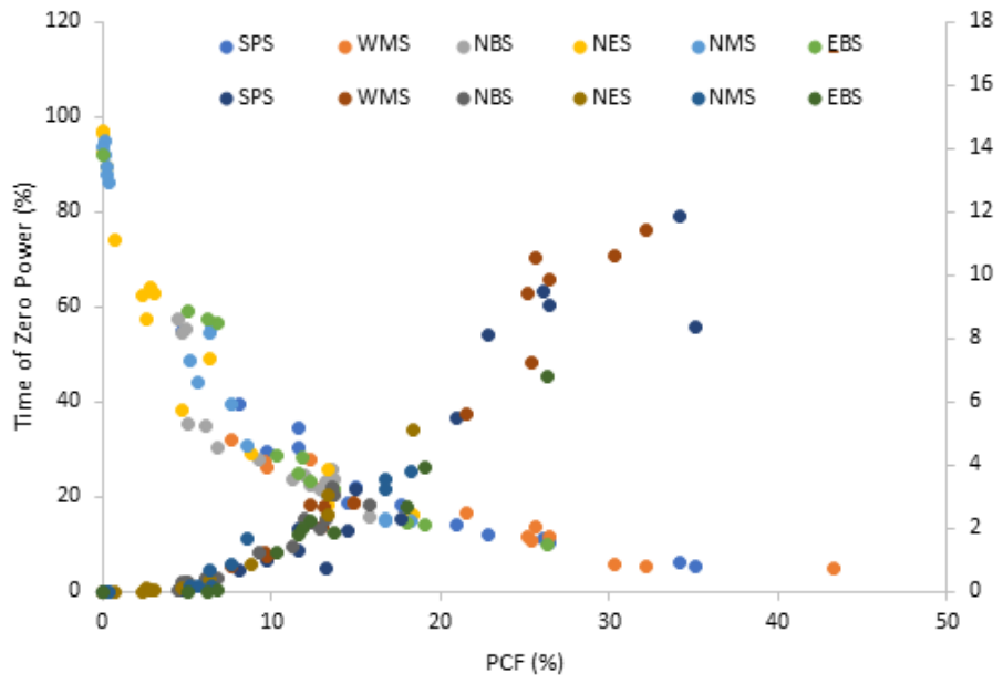
Figure 13 provides an understanding of the relationship between PCF (%) and the corresponding value of Time to Zero Power (%), considering the various methods employed, i.e., SPS, WMS, NBS, NES, NMS, and EBS, which show the general trend of the dataset. A strong negative correlation is observed, which indicates that when PCF is low, i.e., within the range of 0–5%, the value of Time to Zero Power is very high, i.e., within the range of 80–100%. This indicates the ability of the system to retain power for a longer period before reaching zero. When PCF increases from 5% to 20%, a sharp decline in the value of Time to Zero Power is observed, which indicates the ability of the system to reduce the time taken to reach zero power when PCF increases, i.e., the system decays faster when PCF is high. When the value of PCF increases from 20 to 25%, the value of Time to Zero Power stabilizes in the range of below 20%, which indicates the ability of the system to stabilize when PCF increases; i.e., the system becomes stable when PCF increases. Considering the various methods employed, i.e., SPS, WMS, NBS, NES, NMS, and EBS, the techniques show a high degree of variability in the range of PCF, i.e., SPS and WMS, which indicates the sensitivity of these methods to the changing value of PCF. On the other hand, the other methods, i.e., NBS, NES, and EBS, show a high degree of clustering, which indicates the stability of the results obtained. The scatter plot indicates the importance of PCF as a controlling parameter, which influences the performance of the system; i.e., the system decays faster when PCF increases, and the value of PCF is high.

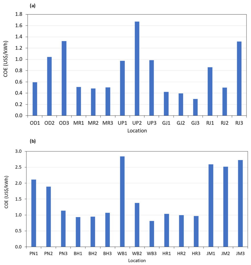
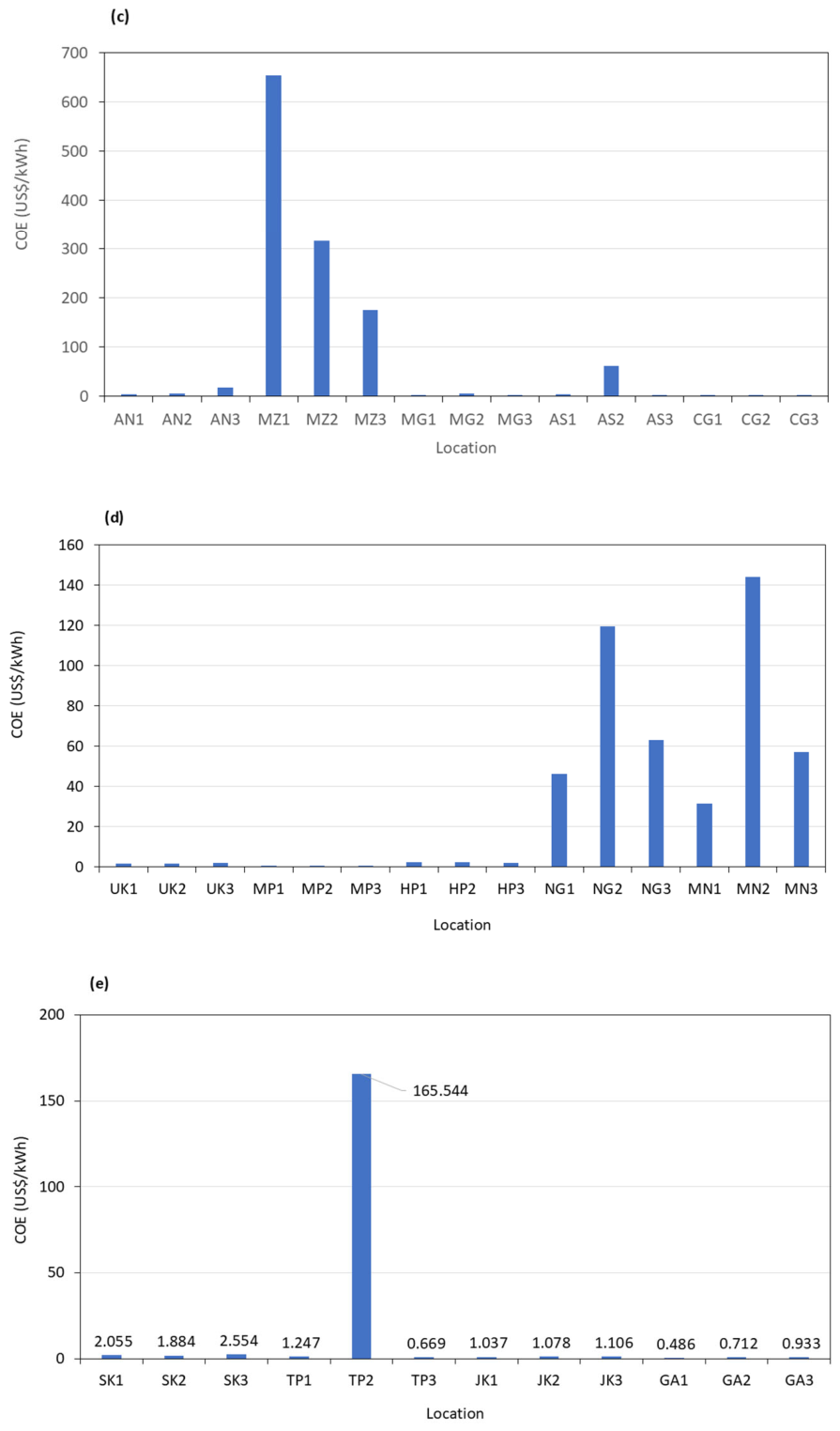
Figure 14 shows a comparative analysis of the COE in various selected regions, highlighting spatial variations in energy economics. The spatial distribution of economic footprints indicates that the COE is not constant and differs significantly depending on various factors, including regional factors. Regions with low energy costs tend to enjoy abundant energy resources, effective energy production mechanisms, and better energy transmission infrastructure. Conversely, regions with higher energy costs tend to experience problems such as scarce energy resources, higher energy consumption, inefficient energy production mechanisms, and poor energy transmission infrastructure. Another factor that contributes to the variation in energy costs among various regions is the variation in energy mixes that each region has adopted [3,9,33,41]. Regions that use alternative energy sources, such as solar, wind, and hydro energy, tend to experience moderate to high energy costs, which may vary with time. Regions that use conventional energy sources tend to experience fluctuating energy costs depending upon various factors, including market prices. Thus, from Figure 14, one can conclude that region-specific energy planning and optimization strategies play a significant role in energy economics. The above analysis has been made by keeping in view the importance of energy economics and how one can use this concept to promote alternative energy sources, which would be more sustainable and cost-efficient.

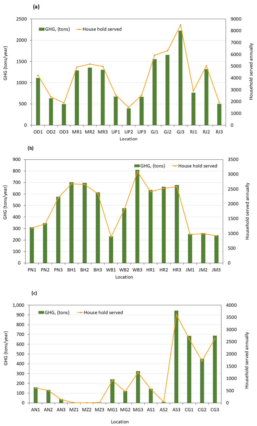
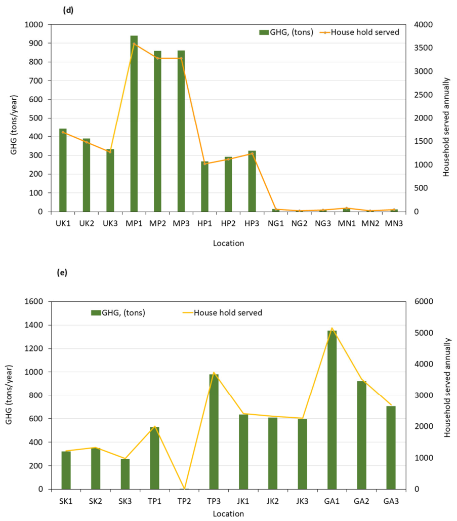
In the pursuit of energy resource exploration and harvesting, many intrinsic correlations exist between total GHG emissions and expected energy utilization in the context of wind farms. For the selected regions of India, one can easily perceive obvious differences between the various regions with regard to the efficiency of energy utilization while maintaining environmental sustainability (Figure 15). Regions with high GHG emissions are the ones with high energy utilization due to the use of fossil fuels in the region’s energy system. This metric is the carbon footprint of the region’s energy system, which is normally a result of traditional energy production methods like the use of coal and oil as a source of energy. On the other hand, regions with low GHG emissions and high energy utilization are those that have shifted towards a cleaner and more sustainable source of energy. One of the most important observations from this study is the decoupling of the GHG emissions and energy utilization of the selected regions. This evidences the efficiency of the energy system of the region with regard to environmental sustainability, the use of cleaner sources of energy, and the effectiveness of the environmental policies of the region [42]. On the other hand, the regions with high GHG emissions and high energy utilization are the ones with a high carbon footprint, and thus, there is a need to reform the energy system and policies of the region with regard to environmental sustainability. The results indicate the significance of the shift towards a low-carbon footprint energy system while maintaining the required level of energy supply and utilization in the region.

In summary, the performance of the selected sites for sustainable wind power production potential can be evaluated under two categories—exploration and extraction. The exploration phase comprises a reliable assessment of wind flow patterns, while the extraction phase consists of effective transformation for useful power production. In this aspect,

Table 1. Comparison of best-performing sites in Indian states based on exploration and extraction scenarios.

State	Sites (with Ranking)
	I	II	III	I	II	III	I	II	III
	Site Notations			PCF (%)			Mean WS (m/s)
Gujarat	GJ3	GJ2	GJ3	43.36	32.24	30.28	7.12	6.25	6.08
Tamil Nadu	TN1	-	-	35.11	-	-	6.40	-	-
Andhra Pradesh	AP2	AP1	AP3	34.24	26.13	20.97	6.37	5.66	5.09
Karnataka	KT1	-	-	26.48	-	-	5.81	-	-
Maharashtra	MR2	MR3	MR1	26.44	25.44	25.14	5.68	5.50	5.53
Goa	GA1	-	-	26.37	-	-	5.59	-	-
Rajasthan	RJ2	-	-	25.70	-	-	5.54	-	-
Telangana	TG2	-	-	22.79	-	-	5.35	-	-
Odisha	OD1	-	-	21.61	-	-	5.03	-	-

shows the three best-performing sites from the top nine Indian states based on mean wind speed as well as plant capacity factor. All three sites from the states of Gujarat, Andhra Pradesh, and Maharashtra show significant performance metrics, while only one site each from the remaining states shows comparative potential (Table 1).

Most previous investigations evaluate wind-resource potential using individual metrics, often emphasizing either statistical wind characteristics or energy-production indicators. In contrast, the proposed framework combines wind speed distribution characteristics, energy potential metrics, and techno-economic performance measures within a standardized rating scheme, thereby enabling a comprehensive comparison of site suitability. However, it should be understood that direct interpretation of the various performance measures of this ranking framework should be done with due consideration of the external factors governing the physical processes of wind flow. This is particularly significant in the case of Indian states with multiple levels of heterogeneous features governing wind power production estimates. Hence, further studies are required to elucidate a detailed scope for dynamically tapping the wind resource from potential sites despite their variability in rating-based rankings.

4. Conclusions

The prediction of the potential for offshore wind energy production in terms of wind power density (WPD) invariably depends on the availability of accurate weather data (precisely, wind speed and direction), topographic conditions (like slope and elevation), and the operational attributes of the wind farm (such as turbine types and operating features). The present study offers a comprehensive evaluation of wind speed characteristics and wind power potential for India on different scales, both temporally and spatially, distributed under six regions. The results provide evidence on the scale dependency of wind patterns, particularly on a daily scale due to local atmospheric conditions such as land–sea breezes, orographic effects, and surface temperature effects. When averaged over larger scales (months or years), wind patterns tend to follow a regular pattern, largely controlled by monsoon winds. In terms of wind power production potential, the Southern Peninsular States (SPSs) and Western Marginal States (WMSs) are more favorable than other regions, with higher wind speeds and less fluctuation. Regions such as the NESs and NBSs are less favorable, with lower wind availability and more fluctuation, restricting their use for large-scale wind energy exploitation.

This study delineates, for the first time, a base-level screening methodology for identifying potential sites in the Indian subcontinent, complementarily mapped with production strategies using rating parameters. The results also invalidate the preconception of the direct dependency of wind energy potential on altitude, as complex terrain and local atmospheric effects tend to produce fluctuations in wind patterns irrespective of altitude. The use of wind variability indices (WVI and WSI) has elucidated the causal factors in a better understanding of wind energy exploitation. This study prioritizes regions with higher frequencies of favorable wind conditions for further exploration over those with occasional extreme wind conditions. The performance criteria, such as PCF, COE, and GHG emissions, also indicate a positive correlation with wind energy exploitation, where regions with higher PCF tend to perform better, with less inefficiency, and also tend to emit fewer greenhouse gases, leading to a cleaner energy transition. The results can be helpful in furthering the operational strategies of upcoming wind farms for sustainable power production.

References

1. IEA. Available online: https://www.iea.org/reports/global-energy-review-2025/co2-emissions (accessed on 21 December 2025).
2. PIB Delhi. Available online: https://www.pib.gov.in/PressReleasePage.aspx?PRID=2183866&reg=3&lang=2 (accessed on 21 December 2025).
3. Ramzan, M.; Larvoe, N.; Mustapa, M.A.C.; Fiankor, D.D.D. Economic Resilience Under Sustainability Uncertainty: Wavelet Quantile Insights from Energy Crises, Oil Market Volatility, and Supply Chain Disruptions. Sustain. Dev. 2026, 1–26. [Google Scholar] [CrossRef]
4. Rehman, S.; Halawani, T.O.; Mohandes, M. Wind power cost assessment at twenty locations in the kingdom of Saudi Arabia. Renew. Energy 2003, 28, 573–583. [Google Scholar] [CrossRef]
5. Singh, U.; Rizwan, M.; Malik, H.; García Márquez, F.P. Wind energy scenario, success and initiatives towards renewable energy in India—A review. Energies 2022, 15, 2291. [Google Scholar] [CrossRef]
6. Clifton, A.; Barber, S.; Stökl, A.; Frank, H.; Karlsson, T. Research challenges and needs for the deployment of wind energy in hilly and mountainous regions. Wind Energy Sci. 2022, 7, 2231–2254. [Google Scholar] [CrossRef]
7. Hunt, K.M.; Bloomfield, H.C. Quantifying renewable energy potential and realized capacity in India: Opportunities and challenges. Meteorol. Appl. 2024, 31, e2196. [Google Scholar] [CrossRef]
8. Wang, W.; Chen, F. Wind field modeling over hilly terrain: A review of methods, challenges, limitations, and future directions. Appl. Sci. 2025, 15, 10186. [Google Scholar] [CrossRef]
9. Thapar, S.; Sharma, S.; Verma, A. Key determinants of wind energy growth in India: Analysis of policy and non-policy factors. Energy Policy 2018, 122, 622–638. [Google Scholar] [CrossRef]
10. John, S.S.; Sony, H.A.; Michael, A.V.; Ramachandran, S. Empowering India Toward Sustainability: An In-Depth Review of Wind Energy Utilization. In Artificial Intelligence for Energy Management; John Wiley & Sons: Hoboken, NJ, USA, 2025; pp. 399–414. [Google Scholar] [CrossRef]
11. WWEA. Available online: https://wwindea.org/GlobalStatistics (accessed on 11 November 2025).
12. IRENA. Available online: https://www.irena.org/Energy-Transition/Technology/Wind-energy (accessed on 11 November 2025).
13. Khaleel, M.; Yusupov, Z.; Rekik, S. Exploring trends and predictions in renewable energy generation. Energy 360 2025, 4, 100030. [Google Scholar] [CrossRef]
14. ICED. Available online: https://iced.niti.gov.in/energy/electricity/generation/pipeline-capacity/wind (accessed on 12 January 2026).
15. NIWE. Available online: https://maps.niwe.res.in/media/150m-report.pdf (accessed on 12 January 2026).
16. Dawn, S.; Tiwari, P.K.; Goswami, A.K.; Singh, A.K.; Panda, R. Wind power: Existing status, achievements and government’s initiative towards renewable power dominating India. Energy Strategy Rev. 2019, 23, 178–199. [Google Scholar] [CrossRef]
17. Akpinar, E.K.; Akpinar, S. An assessment on seasonal analysis of wind energy characteristics and wind turbine characteristics. Energy Convers. Manag. 2005, 46, 1848–1867. [Google Scholar] [CrossRef]
18. Delina, L.L. Wind energy in the city: Hong Kong’s offshore wind energy generation potential, deployment plans, and ecological pitfalls. Electr. J. 2022, 35, 107139. [Google Scholar] [CrossRef]
19. Jowder, J.A.L. Wind power analysis and site matching of wind turbine generators in kingdom of Bahrain. Appl. Energy 2009, 86, 538–545. [Google Scholar] [CrossRef]
20. Gao, Q.; Bechlenberg, A.; Jayawardhana, B.; Ertugrul, N.; Vakis, A.I.; Ding, B. Techno-economic assessment of offshore wind and hybrid wind–wave farms with energy storage systems. Renew. Sustain. Energy Rev. 2024, 192, 114263. [Google Scholar] [CrossRef]
21. Hossain, M.S.; Islam, S.; Sultana, K.R.; Fuhad, M.A. Feasibility study of wind energy in Bangladesh: A way towards sustainable development. In Proceedings of the International Conference on Environmental Technology and Construction Engineering for Sustainable Development, Sylhet, Bangladesh, 10–12 March 2011; ICETCESD: Sylhet, Bangladesh, 2011. [Google Scholar]
22. Vasudevan, M.; Natarajan, N.; Kumar, E.S.; Tamizharasu, S.; Rehman, S.; Alhems, L.M.; Alam, M.M. Environmental and socio-economic aspects of public acceptance of wind farms in Tamil Nadu, India–key observations and a conceptual framework for social inclusion. Pol. J. Environ. Stud. 2023, 32, 3339–3353. [Google Scholar] [CrossRef] [PubMed]
23. Natarajan, N.; Rehman, S.; Nandhini, S.S.; Vasudevan, M. Evaluation of Wind Energy Potential of the State of Tamil Nadu, India Based on Trend Analysis. FME Trans. 2021, 49, 244–251. [Google Scholar] [CrossRef]
24. Rehman, S.; Natarajan, N.; Vasudevan, M.; Alhems, L.M. Assessment of wind energy potential across varying topographical features of Tamil Nadu, India. Energy Explor. Exploit. 2020, 38, 175–200. [Google Scholar] [CrossRef]
25. Boopathi, K.; Kushwaha, R.; Balaraman, K.; Bastin, J.; Kanagavel, P.; Prasad, R.D.M. Assessment of wind power potential in the coastal region of Tamil Nadu, India. Ocean Eng. 2021, 219, 108356. [Google Scholar] [CrossRef]
26. Chandel, S.S.; Ramasamy, P.; Murthy, K.S.R. Wind power potential assessment of 12 locations in western Himalayan region of India. Renew. Sustain. Energy Rev. 2014, 39, 530–545. [Google Scholar] [CrossRef]
27. Natarajan, N.; Vasudevan, M.; Rehman, S. Evaluation of suitability of wind speed probability distribution models: A case study from Tamil Nadu, India. Environ. Sci. Pollut. Res. 2022, 29, 85855–85868. [Google Scholar] [CrossRef] [PubMed]
28. Shukla, K.K.; Natarajan, N.; Vasudevan, M. Comparison of wind speed probability distribution models for accurate evaluation of wind energy potential: A case study from Kerala, India. J. Inst. Eng. (India) Ser. A 2023, 104, 551–563. [Google Scholar] [CrossRef]
29. Sakuru, S.K.V.S.; Ramana, M.V. Wind power potential over India using the ERA5 reanalysis. Sustain. Energy Technol. Assess. 2023, 56, 103038. [Google Scholar] [CrossRef]
30. Gonçalves, M.; Martinho, P.; Soares, C.G. A 33-Year Hindcast on Wave Energy Assessment in the Western French Coast. Energy 2018, 165, 790–801. [Google Scholar] [CrossRef]
31. El Khchine, Y.; Sriti, M.; Elyamani, N.E.E.K. Evaluation of Wind Energy Potential and Trends in Morocco. Heliyon 2019, 5, e01830. [Google Scholar] [CrossRef] [PubMed]
32. Kamranzad, B.; Etemad-Shahidi, A.; Chegini, V. Developing an Optimum Hotspot Identifier for Wave Energy Extracting in the Northern Persian Gulf. Renew. Energy 2017, 114, 59–71. [Google Scholar] [CrossRef]
33. Shi, R.J.; Fan, X.C.; He, Y. Comprehensive evaluation index system for wind power utilization levels in wind farms in China. Renew. Sustain. Energy Rev. 2017, 69, 461–471. [Google Scholar] [CrossRef]
34. Bonthu, S.; Purvaja, R.; Singh, K.S.; Ganguly, D.; Muruganandam, R.; Paul, T.; Ramesh, R. Offshore wind energy potential along the Indian Coast considering ecological safeguards. Ocean Coast. Manag. 2024, 249, 107017. [Google Scholar] [CrossRef]
35. Singh, R.; Jaiswal, N.; Kishtawal, C.M. Rising surface pressure over Tibetan Plateau strengthens Indian summer monsoon rainfall over northwestern India. Sci. Rep. 2022, 12, 8621. [Google Scholar] [CrossRef] [PubMed]
36. Joshi, S.K.; Kumar, S.; Sinha, R.; Rai, S.P.; Khobragade, S.; Rao, M.S. Identifying moisture transport pathways for north-west India. Geol. J. 2023, 58, 4428–4440. [Google Scholar] [CrossRef]
37. Acharya, S. Analytic assessment of renewable potential in Northeast India and impact of their exploitation on environment and economy. Environ. Sci. Pollut. Res. 2022, 29, 29704–29718. [Google Scholar] [CrossRef] [PubMed]
38. Roga, S.; Dahiwale, H.; Bardhan, S.; Sinha, S. Wind energy potential assessment: A case study in Central India. Proc. Inst. Civ. Eng.-Energy 2024, 177, 130–148. [Google Scholar] [CrossRef]
39. Yadav, H.K.; Yadav, S.; Gupta, M.N.; Sarkar, A.; Sarkar, J. Diurnal variations in wind power density analysis for optimal wind energy integration in different Indian sites. Sustain. Energy Technol. Assess. 2024, 64, 103744. [Google Scholar] [CrossRef]
40. Bastin, J.; Katyal, R.; Vinod Kumar, R.; Yuvasri Lakshmi, P. Inter Annual Variability of wind speed in India. Int. J. Ambient. Energy 2022, 43, 5232–5246. [Google Scholar] [CrossRef]
41. Wimhurst, J.J.; Nsude, C.C.; Greene, J.S. Standardizing the factors used in wind farm site suitability models: A review. Heliyon 2023, 9, e15903. [Google Scholar] [CrossRef] [PubMed]
42. Kumar, A.; Pal, D.; Kar, S.K.; Mishra, S.K.; Bansal, R. An overview of wind energy development and policy initiatives in India. Clean Technol. Environ. Policy 2022, 24, 1337–1358. [Google Scholar] [CrossRef] [PubMed]
Figure 1. (a) Global trends in wind energy production capacity (GW) during the last decade and (b) top contributing countries in global wind energy production based on the total installed capacity (GW) during the last two decades.
Wind 06 00034 g001
Figure 2. Comparison of estimated wind potential for the windy states of India at hub heights of 100 m and 120 m. The bullets indicate the updated installed capacity.
Wind 06 00034 g002
Figure 3. Details of selected locations across six regions categorized for the Indian states.
Wind 06 00034 g003
Figure 4. Trend of correlation between the altitude and wind speed values for the selected locations. [CRMC = Cube-Root Mean Cubed].
Wind 06 00034 g004
Figure 5. Flow diagram indicating the methodology used in the present analysis.
Wind 06 00034 g005
Figure 6. Diurnal variations in the wind speed for the selected regions: (a) SPS, (b) WMS, (c) NBS, (d) NES, (e) NMS, and (f) EBS.
Wind 06 00034 g006aWind 06 00034 g006b
Figure 7. Mean monthly variations in the wind speed for the selected regions: (a) SPS, (b) WMS, (c) NBS, (d) NES, (e) NMS, and (f) EBS.
Wind 06 00034 g007aWind 06 00034 g007b
Figure 8. Mean annual variations in the wind speed for the selected regions: (a) SPS, (b) WMS, (c) NBS, (d) NES, (e) NMS, and (f) EBS.
Wind 06 00034 g008aWind 06 00034 g008b
Figure 9. Wind speed characteristics according to different altitude zones: (a) 0–100 m; (b) 100–500 m; (c) 500–1000 m; (d) 1000–2000 m; (e) >2000 m. The green dashed line indicates overall average value.
Wind 06 00034 g009aWind 06 00034 g009b
Figure 10. Representations of wind speed distribution in India based on (a) average value, (b) maximum value, and (c) Cube-Root Mean Cubed (CRMC) values.
Wind 06 00034 g010aWind 06 00034 g010b
Figure 11. Wind power density characteristics according to different altitude zones: (a) 0–100 m; (b) 100–500 m; (c) 500–1000 m; (d) 1000–2000 m; (e) >2000 m. The red dashed line indicates overall average value.
Wind 06 00034 g011aWind 06 00034 g011b
Figure 12. Comparison of wind variability indices based on (1) monthly (MWVI and MWSI) and (2) annual (AWVI and AWSI) WPD data for the six regions, namely (a) SPS, (b) WMS, (c) NBS, (d) NES, (e) NMS, and (f) EBS.
Wind 06 00034 g012aWind 06 00034 g012bWind 06 00034 g012cWind 06 00034 g012d
Figure 13. Effect of PCF on Time to Zero Power across the six regions, namely SPS, WMS, NBS, NES, NMS, and EBS.
Wind 06 00034 g013
Figure 14. Comparison of COE for the selected regions namely (a) WMS, (b) NBS, (c) NES, (d) NMS, and (e) EBS.
Wind 06 00034 g014aWind 06 00034 g014b
Figure 15. Comparison of total GHG emissions and expected energy utilization for the selected regions namely (a) WMS, (b) NBS, (c) NES, (d) NMS, and (e) EBS.
Wind 06 00034 g015aWind 06 00034 g015b