Aerodynamic Effect of Gurney Flaps on NREL Phase VI Wind Turbine Blade

Abstract

As the population increases, the demand for power continues to rise. As fossil fuel resources reduce, wind energy emerges as a sustainable alternative and helps address adverse effects of global warming and environmental pollution caused by fossil fuels. Thus, this study focuses on increasing the efficiency of wind turbines by improving their energy conversion. In this study, the NREL Phase VI wind turbine blade was modified by adding a Gurney flap at trailing edge along the entire span. Computational fluid dynamics simulations using ANSYS CFX 19.2 were performed on the modified blades to evaluate their aerodynamic performance. Three different flap lengths were investigated with six wind speeds varying from 5 m/s to 20 m/s. The results obtained were compared with those from NREL Phase VI original shape and a blade equipped with a winglet. Computational domain was divided into a rotating cylindrical region and a stationary rectangular part. The aerodynamic parameters calculated include torque, thrust, and normal and tangential forces coefficients. At low velocities, the addition of a Gurney flap had an insignificant impact on torque and thrust, whereas at medium to high wind speeds, significant increases were observed on torque, indicating more power production.

1. Introduction

For centuries, to perform mechanical work humans have harnessed wind energy. The sails of boats used wind energy to propel forward, and later, windmills were used to work in agricultural applications such as grinding and pumping of water. The utilization of windmills decreased as the industrial age turned to fossil fuels for energy resources. The availability of energy is key to industrialization and development in society. An increase in the world population has continued to drive progress towards the automation of several developing countries, and increased energy use by industrialized countries has placed greater demand on energy. As a result, in the last 50 years, energy demand has grown exponentially compared to previous centuries [1]. The world population, which was 7.4 billion in 2015, is expected to grow to 8.4 billion by 2030. Most countries still depend on fossil fuels for their energy needs. However, the present reserve of fossil fuel resources is limited, and because of the increased demand, it is expected to be depleted much earlier than previously predicted. Another critical issue with fossil fuel is the emission of environmental pollutants and greenhouse gases from their combustion. The total greenhouse gas emissions globally in 2010 were 54 Gt CO₂-eq [1n] and are projected to be 70 Gt CO₂-eq in 2050 [2]. This is a serious concern for future generations. Due to the predicted earlier depletion of fossil fuel and its adverse effect on the environment, each nation in the world is very interested in developing an alternative, less polluting form of renewable energy [2]. Wind energy has become a worthy choice due to its reasonably economic feasibility and environmentally friendly nature. Wind energy’s global potential is much higher than the world’s energy demand for all purposes, around 35 times the global electricity [3]. As a result, a sharp increase in demand has increased interest in wind turbines for energy production for several years. For example, in 2014, the installed wind power capacity was more than 50 GW globally, and the total accumulative installations reached 369 GW at the end of that year. In 2016, the full wind power capacity globally reached 486 GW. Therefore, the wind power generation system is considered a promising industrial and scientific research area [3].

Although several studies have investigated the use of Gurney flaps on airfoils and wind turbine blades, most existing work has focused on two-dimensional configurations or sectional blade applications under limited operating conditions. In the present study, the aerodynamic effects of a Gurney flap applied along the entire span of the NREL Phase VI wind turbine blade are examined using three-dimensional numerical simulations. The performance of the Gurney flap modified blade is further compared with that of a blade equipped with a winglet to contrast different aerodynamic performance enhancement approached under identical operating conditions.

Goals and Objectives

The current study’s primary goal is to determine the aerodynamic loads on the NREL Phase VI wind turbine blades with modified designs using Gurney flaps at the trailing edge and compare them with two blade designs.

The following objectives are determined to achieve these goals:

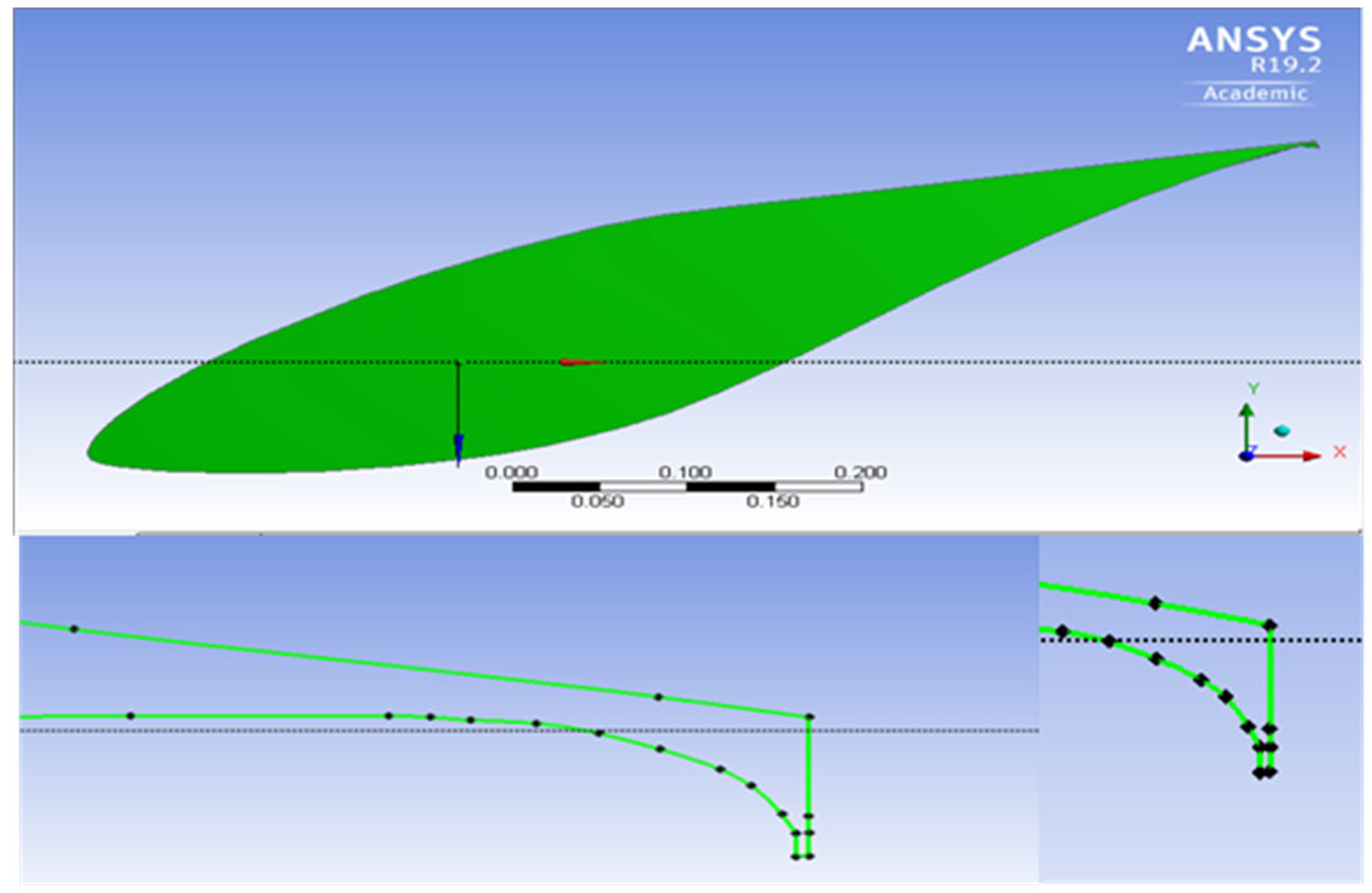
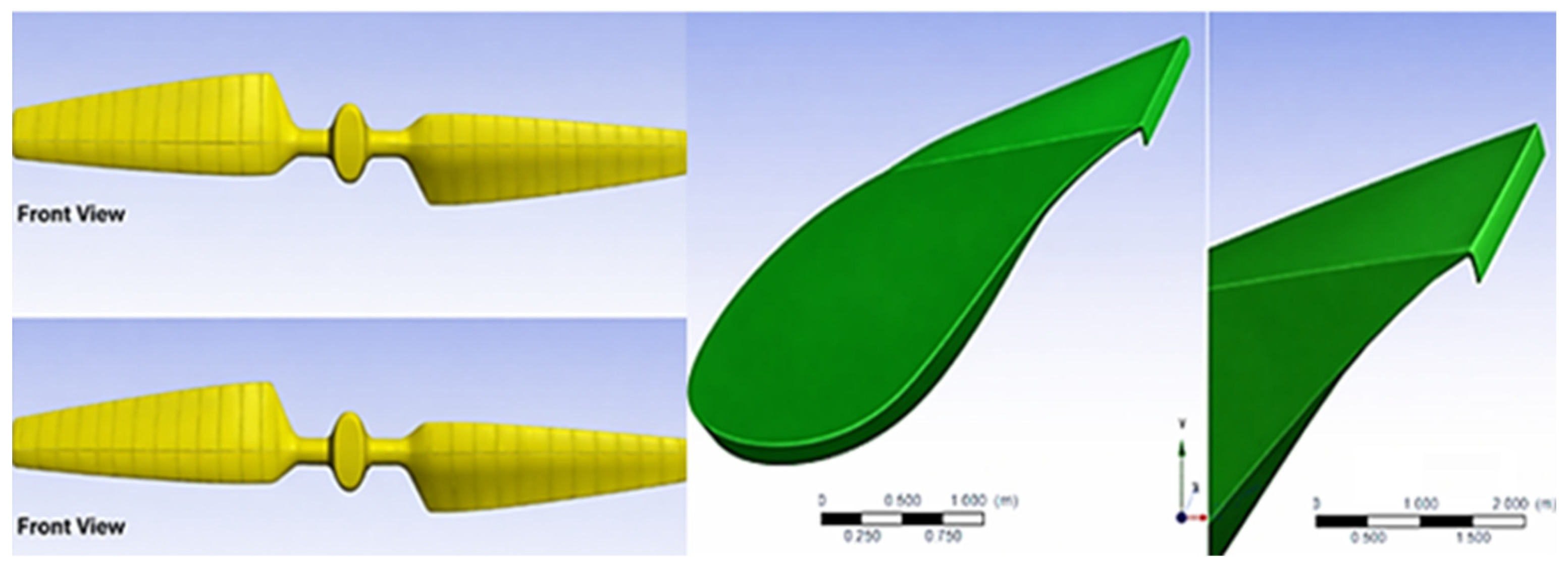
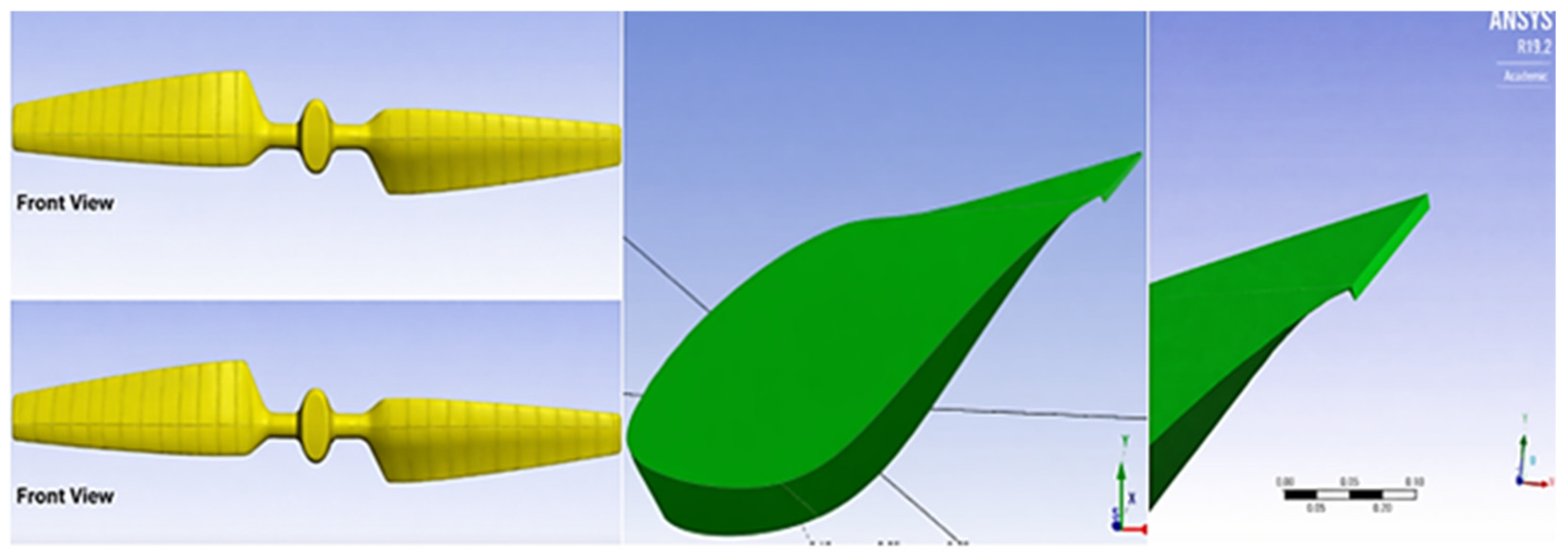
• Alter the design of the National Renewable Energy Laboratory (NREL) Phase VI wind turbine blade by attaching Gurney flaps at the trailing edge.
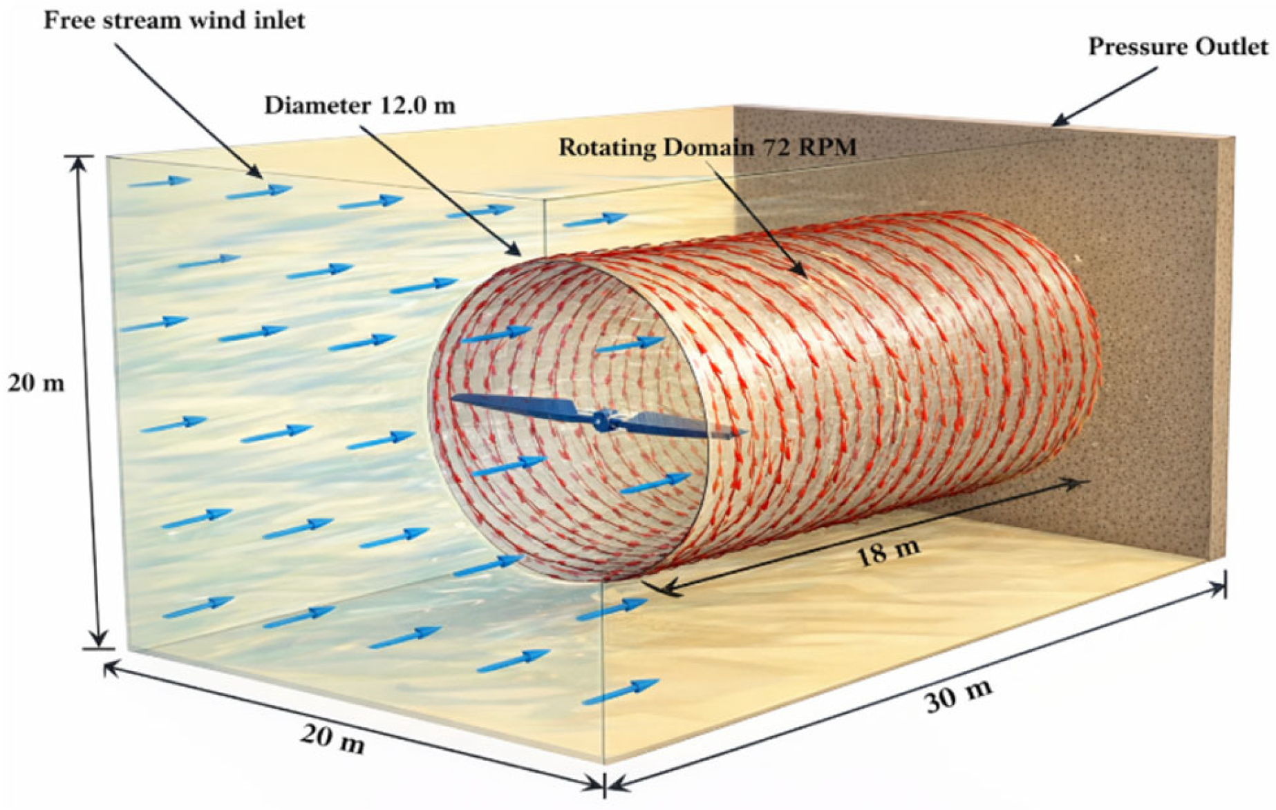
• Use ANSYS CFX as the simulation tool and generate a computational domain based on a cylindrical rotating domain within a fixed rectangular domain while generating a fine grid so that y+ value is less than 1.
• Select the SST turbulence model and determine the velocity coefficient, pressure coefficient, tangential and normal force coefficients for various blade designs and determine the three-dimensional torque and thrust forces generated for each of the designs.

2. Wind Turbine Blade Modifications

Each blade area can be individually designed and calculated to achieve the desired performance characteristics. The following explores some of the design modifications proposed or developed by researchers and some of the performance results. 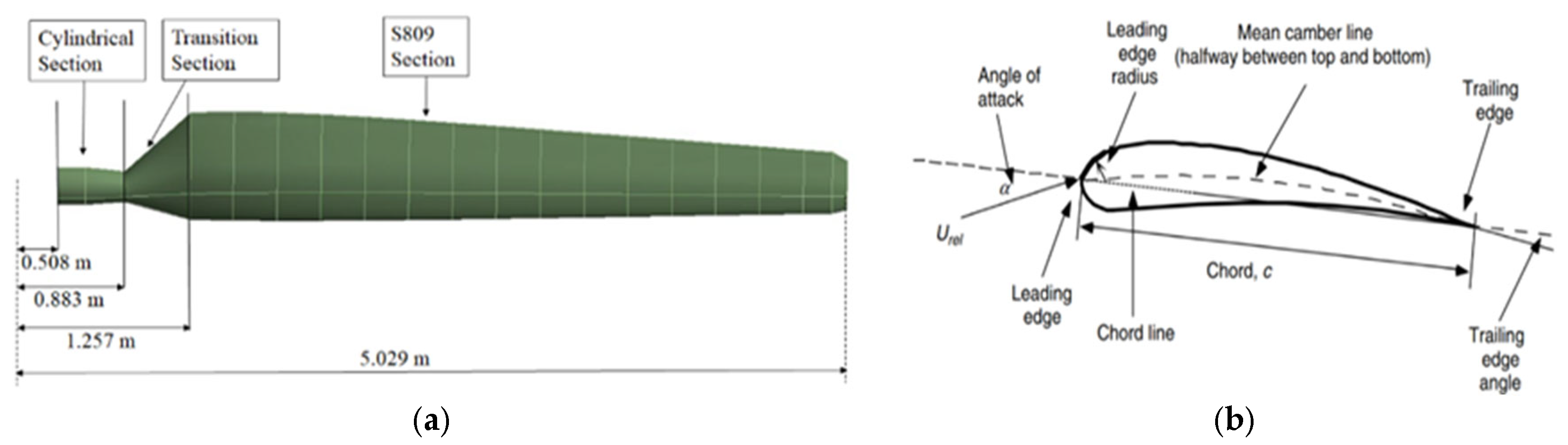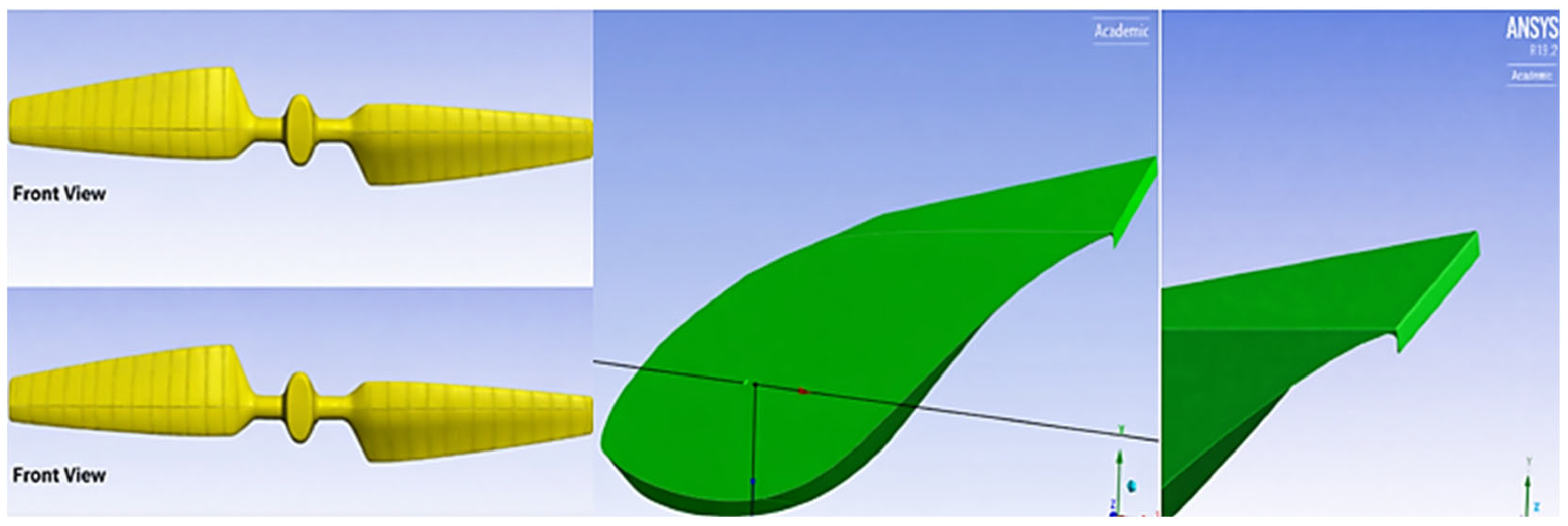Based on the available literature, the improvements can be classified into two types: span-wise modifications and stream-wise modifications, and each change may be either a full or sectional modification device [4]. In full span-wise modification, the entire blade may be modified by changing the associated airfoil shape. Changing the airfoil to different airfoil families will dramatically change the characteristic aerodynamic performance with the same radius and solidity. Airfoil families are classified into thick and thin, depending on the camber distance. The S809 airfoil blade shown in Figure 1a is from a mid-size airfoil family initially designed for aircraft wings [4]. Sectional span-wise modification aims to change structural stability by changing flow circulation over parts of the wing. Hub-root modification is changing the hub design that drastically affects the downstream flow of the rotor. When the rotor has active control over the pitch, a thinner airfoil may reduce turbulent wake vortex rotation structures and improve power generation [4].

Tip modification is changing the tip that has been shown to improve performance and reduce tip vortices slightly. In PVAMU, research on winglets has been presented showing that span-wise modifications and stream-wise modifications can dramatically change the blade’s performance characteristics [4]. Typically, this modification type is a change in the twist angle. On the other hand, the sectional modification of stream-wise modification’s aim is to change the characteristic cross-sectional geometries of the base airfoil. A designer may use this modified airfoil along the entire blade span or only in a particular area such as the root, mid-span, or tip. Several researchers have explored using multiple airfoil geometries. Problems of such complexity may not be fully understood until better prediction algorithms are developed. Figure 1b shows the parts of an airfoil. Each section may be modified in isolation or in conjunction with additional features. Typically, the leading and trailing edges are modified since they are along the circulation stream and have the significant effect on airfoil lift and drag forces [5]. Leading-edge modification leads to changes in the inflow velocity of the freestream wind by disrupting the laminar flow. These devices are vortex generators and can be beneficial. Finally, the current study’s focus is to modify the trailing edge of s809 airfoil, which will change the outflow characteristic of the upper or lower surface. Several devices of this type have been investigated as it is postulated that the separation bubble is stabilized, delayed, the useful chord lengthened, or the span-wise mixing is reduced. Of particular interest is the Gurney flap edge, which marginally increases lift to a maximum in a narrow range before taping into ineffectiveness [5].

Gurney Flap (GF)

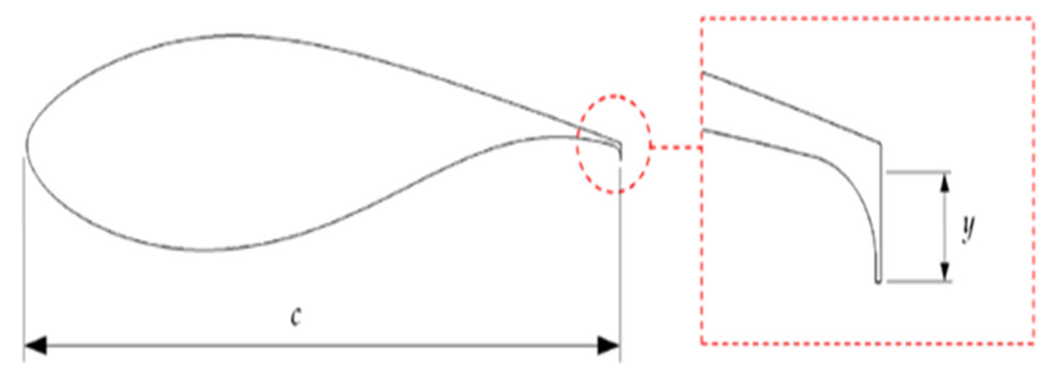
Perhaps the best known yet little understood example of a trailing edge modification device is called the Gurney flap (GF). Originally, the Gurney flap was used on race cars to increase the downward force, lift, which allowed better contact with the road surface as speed increased. On wind turbines, the Gurney flap is postulated to work similarly [6,7,8,9]. The exact mechanism by which the Gurney flap works is not known; instead, flow studies have been conducted to elucidate the flow around the blade [7,10]. The standard Gurney flap is a tab perpendicular to the lower surface between the heights of 0.5% C and 3% C [11].

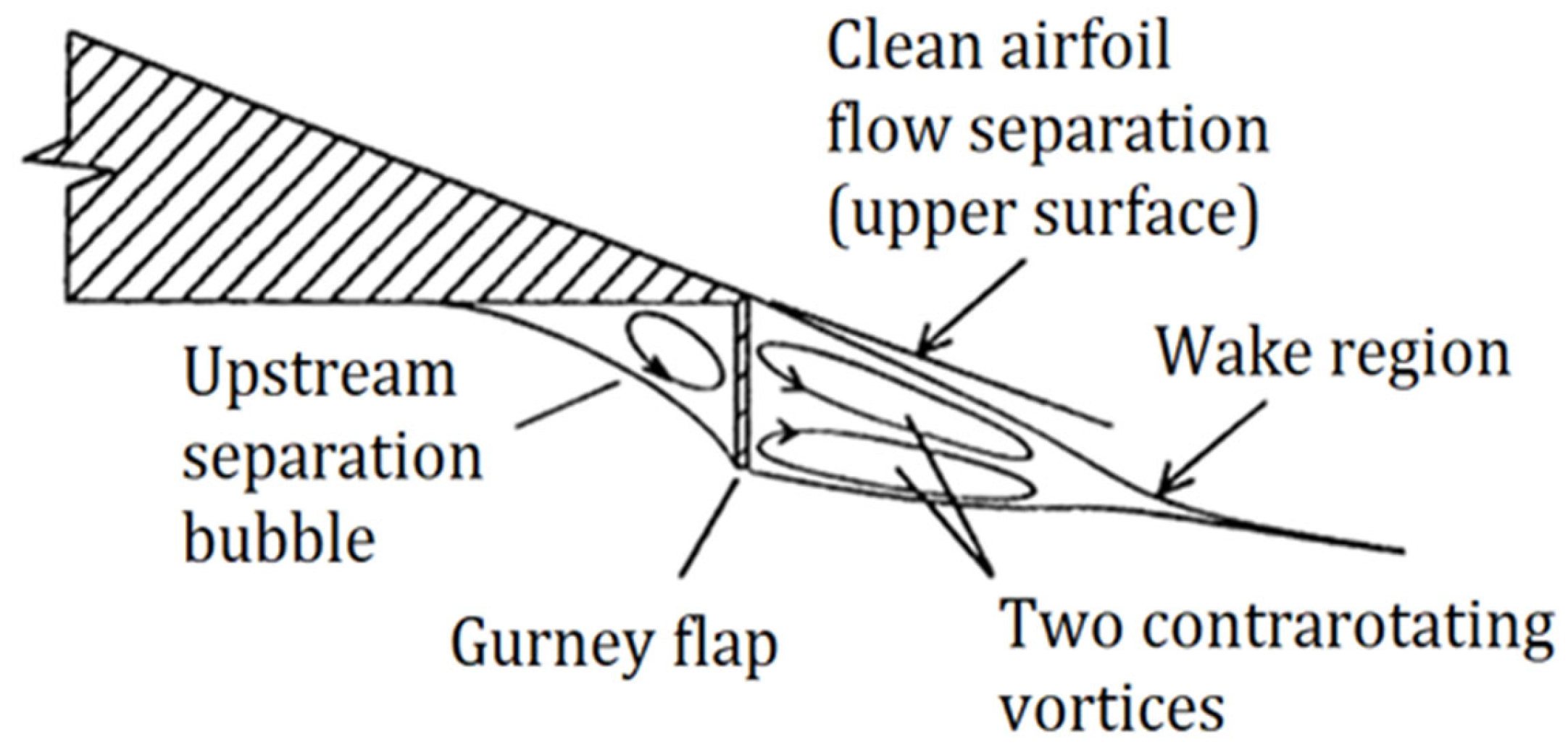
Research has shown that the GF’s most effective parameter is just below 2% C, which effectively increases the lift-to-drag ratio [9,11,12]. Beyond 2% C, the drag coefficient starts rising rapidly. Some researchers postulated that the aerodynamic force alteration was due to a small region of separated flow directly upstream of the flap, two counter-rotating vortices downstream of the flap, and an increased area of the attached flow on the upper-side [6,13,14]. Figure 2 shows the flow around the Gurney flap. The combined flow effects modify the trailing edge Kutta condition and result in infinite pressure differences between the upper and lower surfaces at the trailing edge [13]. The Gurney flap was found to alter the Kutta condition by changing the separation point location at the trailing edge, which provides the airfoil more bound circulation and lifts force [15]. The standard Gurney flap may be modified to have additional flow characteristics. The saw-tooth, perforated, T-stripes or GF with slits were analyzed in [9], divergent plane GF were studied in [8,16], alon with trailing edge devices similar to the GF such as wedge and convexly curved wedge. The GF tab connected to the lower airfoil surface is analyzed in [11]. The difficulty in establishing an exact mechanism of action for the Gurney flap geometries emphasizes why a wind tunnel test is irreplaceable even when coupled with additional simulation routines. 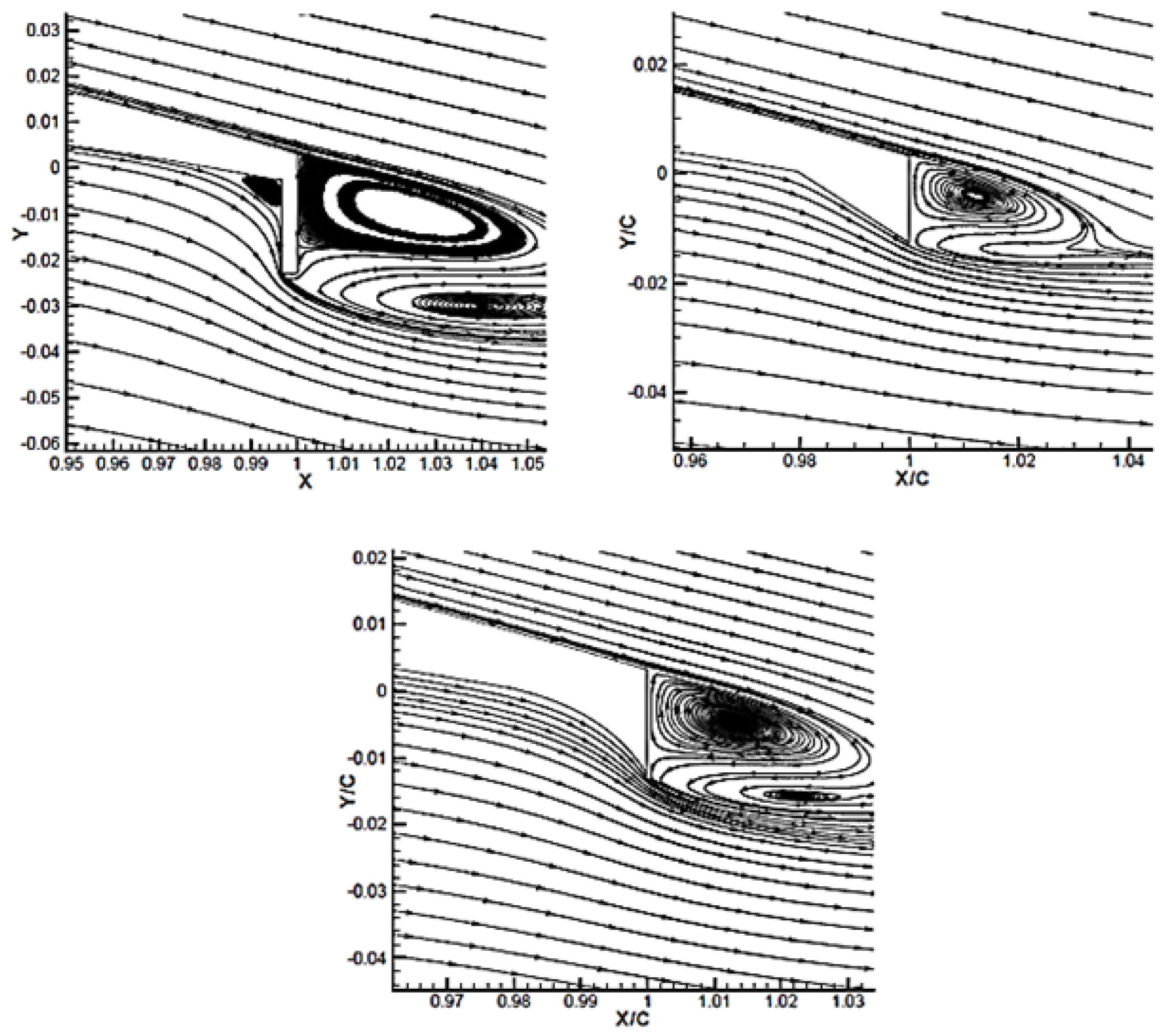Figure 3 shows the three trailing edge devices discussed [10].

3. Methodology

3.1. CFD Workflow and Numerical Framework

The CFD simulations were performed using ANSYS CFX 19.2 following a standard three-stage procedure. It consists of pre-processing, solution, and post-processing. The whole workflow was organized in five algorithmic steps. First, the airfoil, blade, and Gurney flap geometry were shaped using ANSYS DesignModeler (ANSYS Fluent R19.2). Next, the computational domain was discretized by using mesh generation with proper grid resolution. The fluent solver setup was then finalized by defining the fluid properties, boundary conditions and turbulence model. Later, the governing equations were resolved numerically by using an iterative solution model. Finally, the aerodynamic performance was evaluated and visualized in the post-processing stage. This framework confirms numerical stability and physical accuracy in standard CFD best practices [17].

3.2. Modeling Blade with Gurney Flap (Geometry)

The NREL Phase VI blade has been used as a model of the S809 airfoil. That airfoil was obtained from the NASA airfoil database. After, it was imported into Excel (CVS.) and ANSYS DesignModeler to generate 2D geometries [13]. Figure 4 represents two-dimensional geometry.

The Gurney flap (GF) height is defined by:

$$\mathrm{Y}=\mathrm{X}\mathrm{\%}\times \mathrm{C}$$

(1)

Y = height of GF. (unit m)

X = percent of chord length. (%)

C = chord length of the airfoil. (unit m)

Figure 4. 2D of Airfoil S809 with GF [13].

Figure 4. 2D of Airfoil S809 with GF [13].

In this research, three modified geometries of the NREL Phase VI blade were generated where three different heights of GF. 2D models were created. As mentioned above, S809 airfoil was used to create the blade with GF. Previous studies have also investigated the aerodynamic effects of Gurney flaps on wind turbine airfoils, demonstrating improvements in lift and overall aerodynamic performance under certain operating conditions [18]. S809 airfoil coordinates were obtained from the NASA website [19] and uploaded to Excel to create the GF coordinates. The coordinates were imported to ANSYS to model the 2D of GFs. Figure 5 shows the coordinates of the airfoil.

The GF high parameter, which is only various, was selected in three different coordinates, as shown in

Table 1. This table is shown three different coordinates for GF high parameter.

Test ID	Cases for Airfoil S809	GF Length
1	GF Design 1	0.8% C
2	GF Design 2	1.5% C
3	GF Design 3	2.0% C

.

After designing 2D, NERL original wind turbine coordinates were used to model three-dimensional coordinates of GF for three cases, as is shown in Table 1.

ANSYS molder 19.2 was used to create a three-dimensional wind turbine blades design based on the selected 2D designs. All three Gurney flap models have the same thickness as the changing heights, which will be the only parameter. GF design 1 has 0.8% C height and 0.005 mm as a thickness, with the same twist angle as NERL original blade. All the parameters of GF blade design 2 and design 3 remain the same as GF design 1 except the height. For the GF design 2, the height is 1.5% C and GF design 3 is 2% C, as shown in Figure 6, Figure 7 and Figure 8, respectively; the range of flap height is based on the 2D study of the Gurney flap. The three values are chosen to observe the aerodynamic load trends with GF height and to have a basis for future parametric studies.

3.3. Mesh Generation

Total fluid domain was discretized with prism layers near the blade surface. For that, unstructured tetrahedral mesh was used. $5.25\times {10}^6 \mathrm{cells}$ was in the mesh count. That was selected to ensure accuracy while maintaining computational efficiency. See Figure 9 [20]. Near-wall resolution was controlled for maintaining $y^{+}\approx 1$. It was maintained for accurately capturing boundary-layer separation and stall behavior [21]. Figure 10 represents the mesh structures.

3.4. Computational Domain

The computational domain was split into two regions. One is inner cylindrical rotating domain surrounding the wind turbine blade and another one is rectangular stationary domain representing the ambient airflow. This domain configuration allowed simulation of blade rotation in a fixed flow field. The inlet was defined as the rectangular domain’s upstream face. The uniform wind velocities 5, 7, 10, 13, 15, and 20 m/s were applied individually. The rectangular domain downstream face was specified as a constant pressure outlet. The remaining four sides of the rectangular domain were treated as symmetry boundaries. It also minimizes blockage and wall effects. The wind turbine blade surface was modeled as a no-slip wall. It helped to correctly represent viscous flow behavior. This setup confirmed stable and physically realistic flow generated around the rotating blade and wake region. Figure 11 shows all the boundary conditions used [21,22].

3.5. Mesh Sensitivity Analysis

Analyzing the numerical fluid flow through CFD simulations, the total fluid domain was discretized by using an unstructured tetrahedral mesh. Prism inflation layers near the blade surfaces are also used there. This meshing strategy was selected for sufficient near-wall resolution. To maintain a reasonable computational cost for total simulation. The final mesh consisted of approximately 5.25 × 10⁶ cells. It was found to provide grid-independent results for acceptable accuracy.

Near-wall resolution was controlled to maintain y⁺ ≈ 1. That is required for accurate prediction of the viscous sublayer. Using the SST (Shear Stress Transport) turbulence model we tried to maintain such low y⁺ values. It allowed proper resolution of boundary-layer separation and stall behavior. That is critical for aerodynamic performance analysis [21]. Previous studies have shown that large y⁺ values give inaccurate values for near-wall flow prediction. It also shows reducing turbulence modeling performance [23].

Non-dimensional wall distance y⁺ is defined as:

$$y^{+}={\displaystyle \frac{y{u}_{\tau }}{\nu }}$$

(2)

where y represents the distance from the wall to the center of the first cell, ν is for the local kinematic viscosity, and $u_{\tau }$ is demonstrated for the friction velocity, given by:

$$u_{\tau }=\sqrt{{\displaystyle \frac{{\tau }_w}{\rho }}}$$

(3)

where ${\tau }_w$ is for the wall shear stress and ρ is represented by the fluid density.

The mesh was generated using ANSYS Meshing (ANSYS R19.2), utilizing prism layers in the near-wall region. The tetrahedral elements are used in the outer flow field. This framework ensures smooth transition from the wall to the free stream. This preserves solution accuracy as well. After a mesh sensitivity study, the final grid was selected. It is also confirmed that further mesh refinement did not have any significant impact on the aerodynamic force coefficients.

3.6. Boundary Condition

The airflow was assumed to be incompressible and Newtonian flow. All simulations were performed in steady-state conditions. Turbulence influences were modeled using the SST $k–\omega$ turbulence model [24]. This is well suited for capturing boundary-layer separation and near-wall flow behavior. For improving numerical accuracy, a pressure-based coupled solver with second-order spatial discretization was used. Convergence was monitored by the reduction in residuals. It was required to fall below ${10}^{-5}$. It was observed by the stabilization of aerodynamic forces and torque. These convergence criteria are used for the numerical solution. It was required for both stability and physically realistic flow.

3.7. Process Result

Aerodynamic performance was determined by using:

• Pressure contours;
• Velocity streamlines;
• Torque and power coefficients;

All results were visualized using CFX-Post (ANSYS R19.2).

4. Results and Discussion

This CFD analysis provides results for three different wind turbine blades with GFs, design 1, design 2, design 3, and the original blade and the blade with winglets from the previous study. CFD results were obtained by running the simulation of six different wind speeds (5 m/s, 7 m/s, 10 m/s, 13 m/s, 15 m/s, 20 m/s). The purpose of this simulation was to see the effect of adding GFs to the trailing edge of the S809 airfoil by creating the three dimensions of a wind turbine blade with GFs in different shapes. CFD results are pressure coefficient distribution, velocity coefficient distribution, tangential and normal force coefficient, torque and thrust, for all five designs, with all speeds above.

4.1. Distribution Curve of CP

The pressure coefficient (C_P) distribution around the blade at a specific span can be used to understand an airfoil section’s aerodynamic performance. The pressure coefficient was plotted as a function of chord ratio (X/C), a non-dimensional parameter. X is the x-directional distance along the chord from the leading edge of an airfoil, and C is the chord length at that span location. Thus, X/C varies from 0 to 1 at every span location, with the leading edge being 0 and the trailing edge being 1. Based on the definition of C_P, a larger negative value indicates higher pressure. Thus, a larger area bounded by the contour indicates a larger C_P between the pressure side and the suction side and larger force and torque. 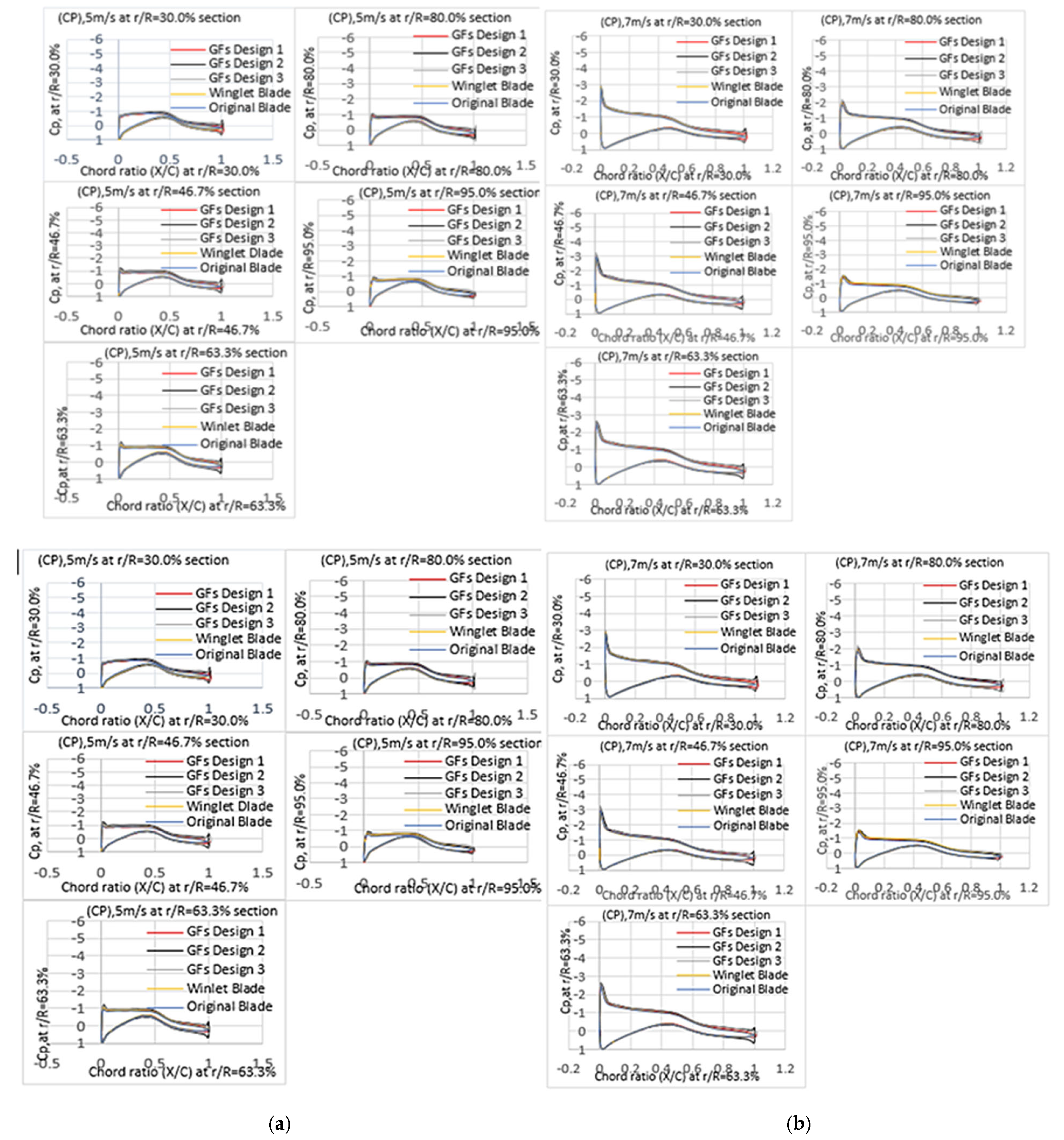This section discusses the C_P contour variation and compares the results from all three flap heights, the original blade, and the blade with the winglet. Comparisons are done at five span locations (0.30%, 0.467%, 0.633%, 0.80%, 0.95%) and six wind velocities (5 to 20 m/s). At a wind speed of 5 m/s, the entire blade span stays in the attached flow region. Since the AoA range is minimal, an insignificant difference in CP distribution is offered at this wind speed of 5 m/s, as shown in Figure 12a, for all the blade shapes and at all five span locations, except at the trailing edge. This small discrepancy is observed at the trailing edge of GF designs due to the presence of GFs, which the contour must trace; this may have some minimal beneficial effect on torque. At 7 m/s, the entire blade is in the transition area within the pre-stall area. Therefore, the Cp distribution at this wind speed also shows tiny variation overall for all five shapes, like the wind speed of 5 m/s. The Cp distributions for this wind speed are shown in Figure 12b. An insignificant amount of variation is observed at 46.7%, 63.3%, and 80% of chord length at the upper curve of GF design 2, near the leading edge. A small variation is observed on the lower Cp curve for all sections of GFs by the trailing edge.

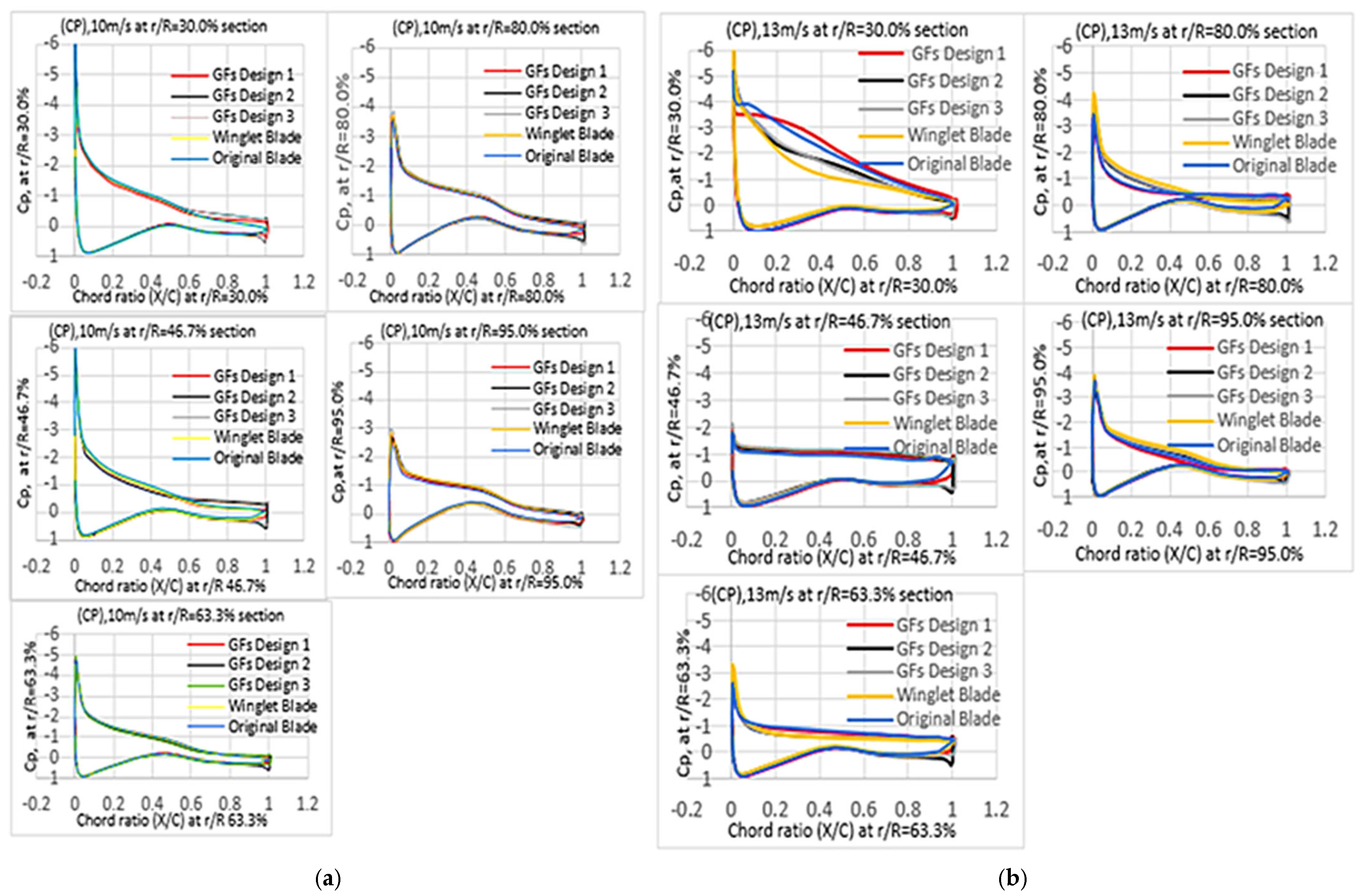
Figure 13a shows the CP distribution at 10 m/s. The base region is in deep stall condition at this speed, including the 30% span section. The mid-section is in a dynamic stall region, including 46.7% span, and the tip region is in transition/separation region or pre-stall region. Near the trailing edge (chord ratio of 0.6 to 1) at both 30% and 46.7% span locations, distinctly larger CP values are observed for GF design 2 and GF design 3. Apart from that, the variations in the designs show an insignificant difference. At this speed, distinctly larger CP values between the pressure side and suction side are observed. Figure 13b also shows the C_P distribution curve of the blade with GF cases, original NREL Phase VI, and blade with a winglet results at 13 m/s wind speed. Around 73% of the blade span from the hub stays in the deep stall region, and the remaining part of the blade remains in the dynamic stall region. The separation between the deep stall region and dynamic stall region takes place at 20⁰ AoA. At 30% span location, GF design 1 exhibits a higher value of C_P compared to all other designs. In comparison, the winglet blade design shows the least amount among the different designs. GFs design 2 and 3 are almost the same but less than the original blade design and GF design 1. The original blade design C_P distribution curve stays between GF design 1 and GFs design 2 and 3. Rest in all span locations, the GF designs, original blade design, and winglet blade design are almost identical but less discrepancy can be observed. However, at span location, 80% in between 0 and 0.4 chord ratio the original design, GF design 1 exhibits lower CP than the others, and greater discrepancy is observed at the tail part of all spans locations because of the GF designs’ blade.

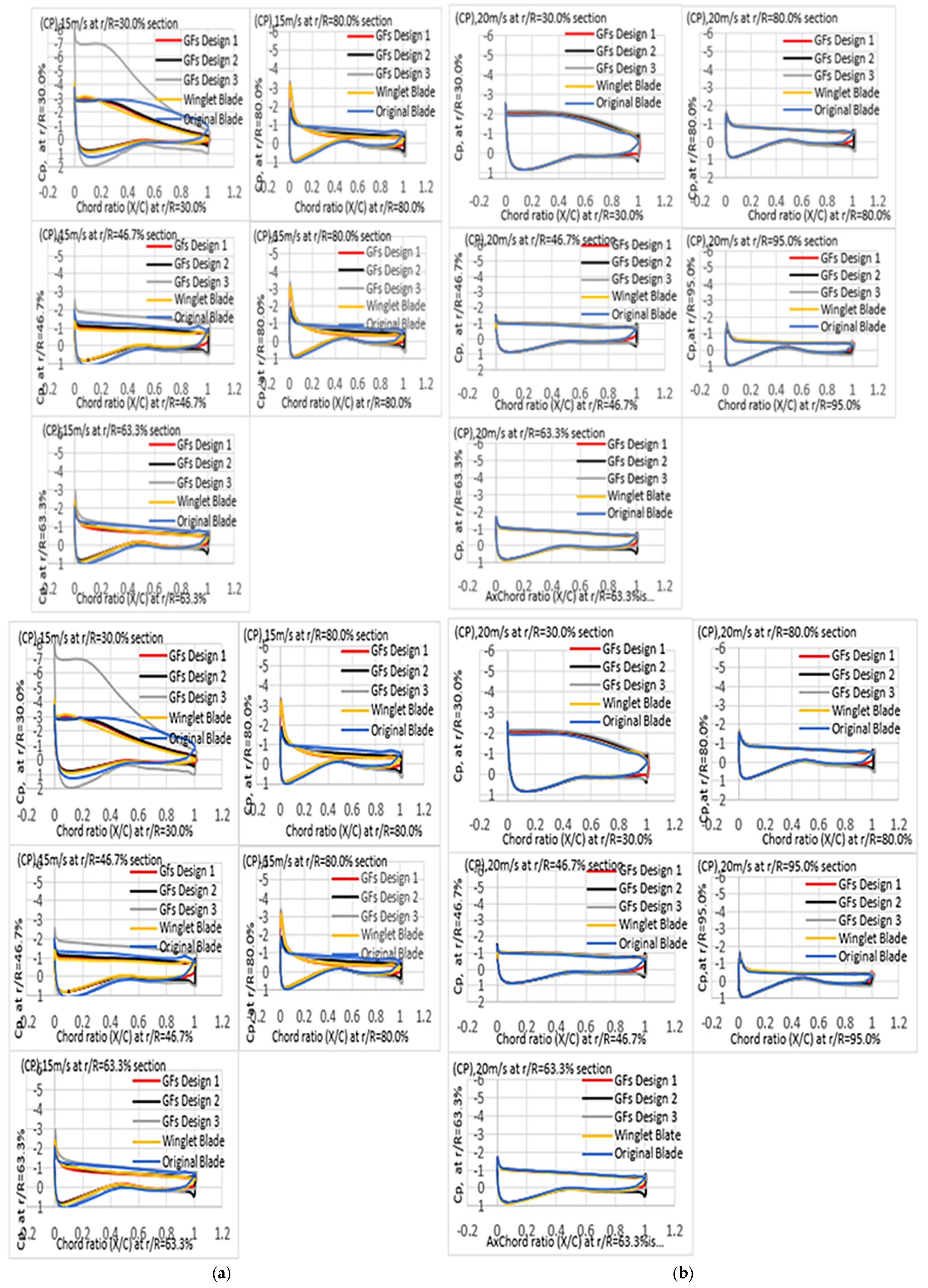
Figure 14a shows the C_P distribution curve for the original NREL VI blade, blade with a winglet, and blade with GF cases for 15 m/s wind speed. Approximately 85% of the blade span from the hub stays in the deep stall region, and the rest of the span remains halted at a dynamic stall region. It also faces the onset of full separation of 20° AoA at a 90% span location. At a 30% blade span, higher negative C_P values are observed from the leading edge up to 0.8 chord ratio for GF design 3. A smaller CP distribution curve is observed for GF design 2 than other designs, and GF design 2 from the leading edge to 0.2 chord ratio shows significantly less value; the rest of the chord had similar values. More negative CP values are shown at 46.7% span location for GF design 3, at 63.3%, 80%, and 95% blade span sections; NREL’s CFD analysis is underpredicted compared to the NREL experimental result. Except the trailing edge, almost the entire CP distribution curve of the original blade, winglet, and GF cases are similar. At 46% span location, GF design 3 performs better than all other designs, and the rest of the designs are almost identical. Again, some discrepancy is observed at the tail part compared to the original blade design and winglet design with all other GF designs. The whole blade span remains within the deep stall region, and flow is fully separated from hub to tip. Therefore, less discrepancy is expected from all C_P distribution curves at 20 m/s in Figure 14b.

4.2. Velocity Coefficient Contour

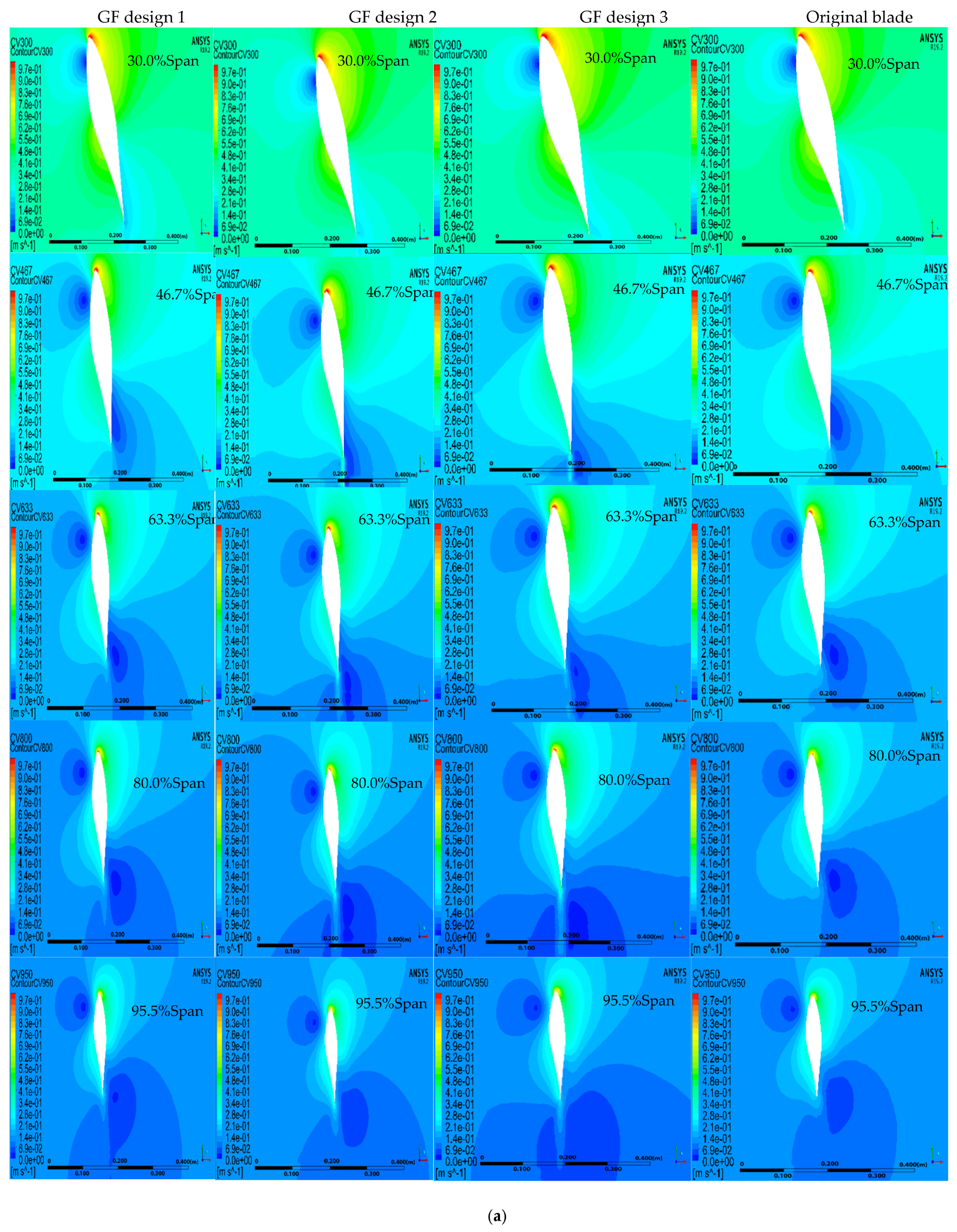
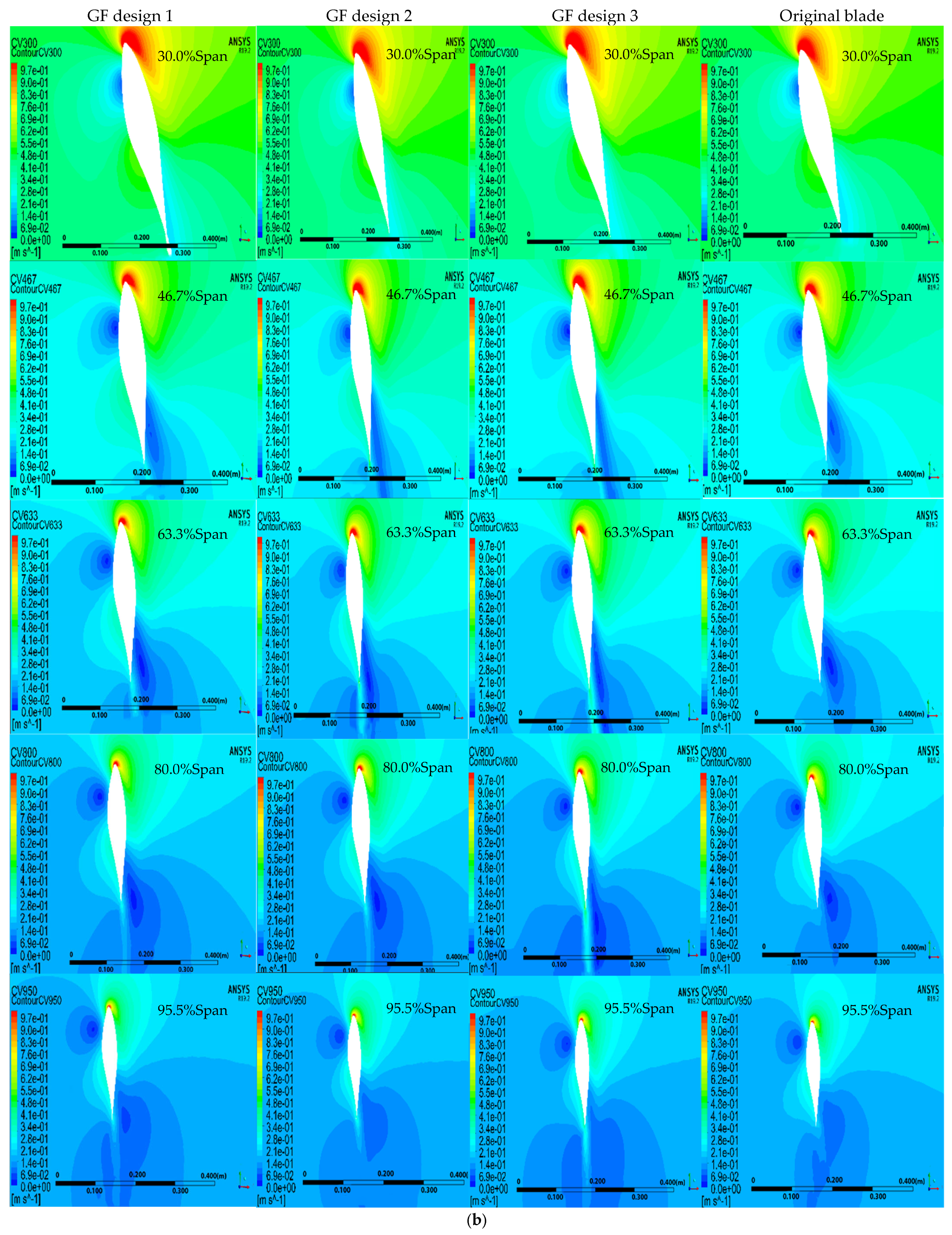
At wind speeds of 5 m/s and 7 m/s, the entire blade span remains within the attached region, and the AoA range, from the hub to the tip is small. The color velocity contour results for all four blade designs are shown in Figure 15a,b for wind speed 5 m/s and for speed 7 m/s, respectively. As observed from the figures, the contours are almost similar for all blade designs and at all span locations except a little difference at the trailing edge of all GFs.

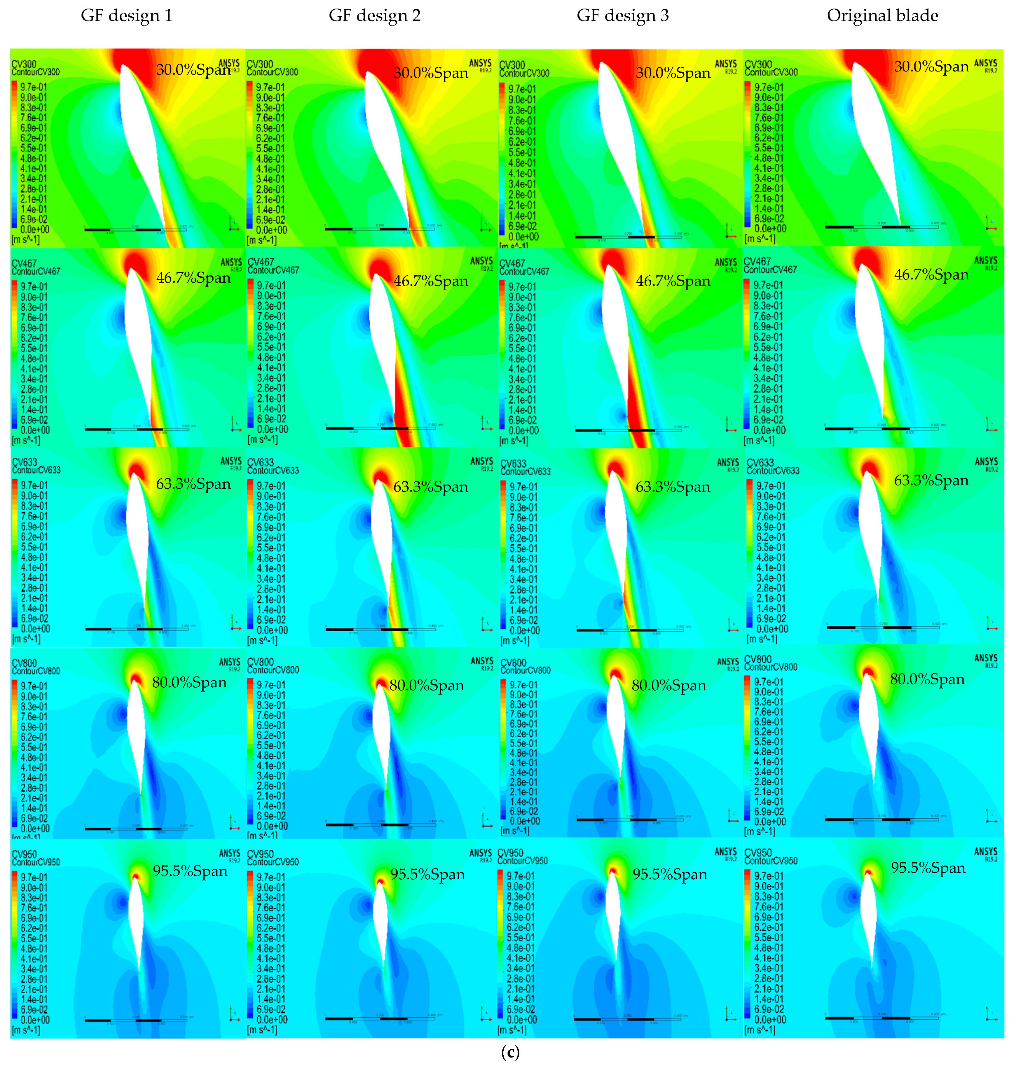
At a wind speed of 10 m/s, some variations between the three GF designs compared to the original blade are observed in the velocity contour. The reason for that is at this speed, Figure 15c, the blade is in three regions. From hub to about 45% of the span is in the deep stall region, where the flow is fully separated. From about 45% to about 75%, the span is in the dynamic stall region, where the flow is partially detached. The rest of the span is in the transition region. The biggest variation in the velocity coefficients among blades is observed in the dynamic stall region for GF designs because of the Gurney flap’s addition. At 30% span blade, comparatively very low separation at suction side trailing edge is observed for all GFs designs. At 46.7% and 63.3%, the blade span ratio shows more separation at the trailing edge for GF design 2 and design 3 than the original blade. At 80% and 95%, the blade’s span sections remain in the pre-stalling region; therefore, the flow is attached for all four blade cases.

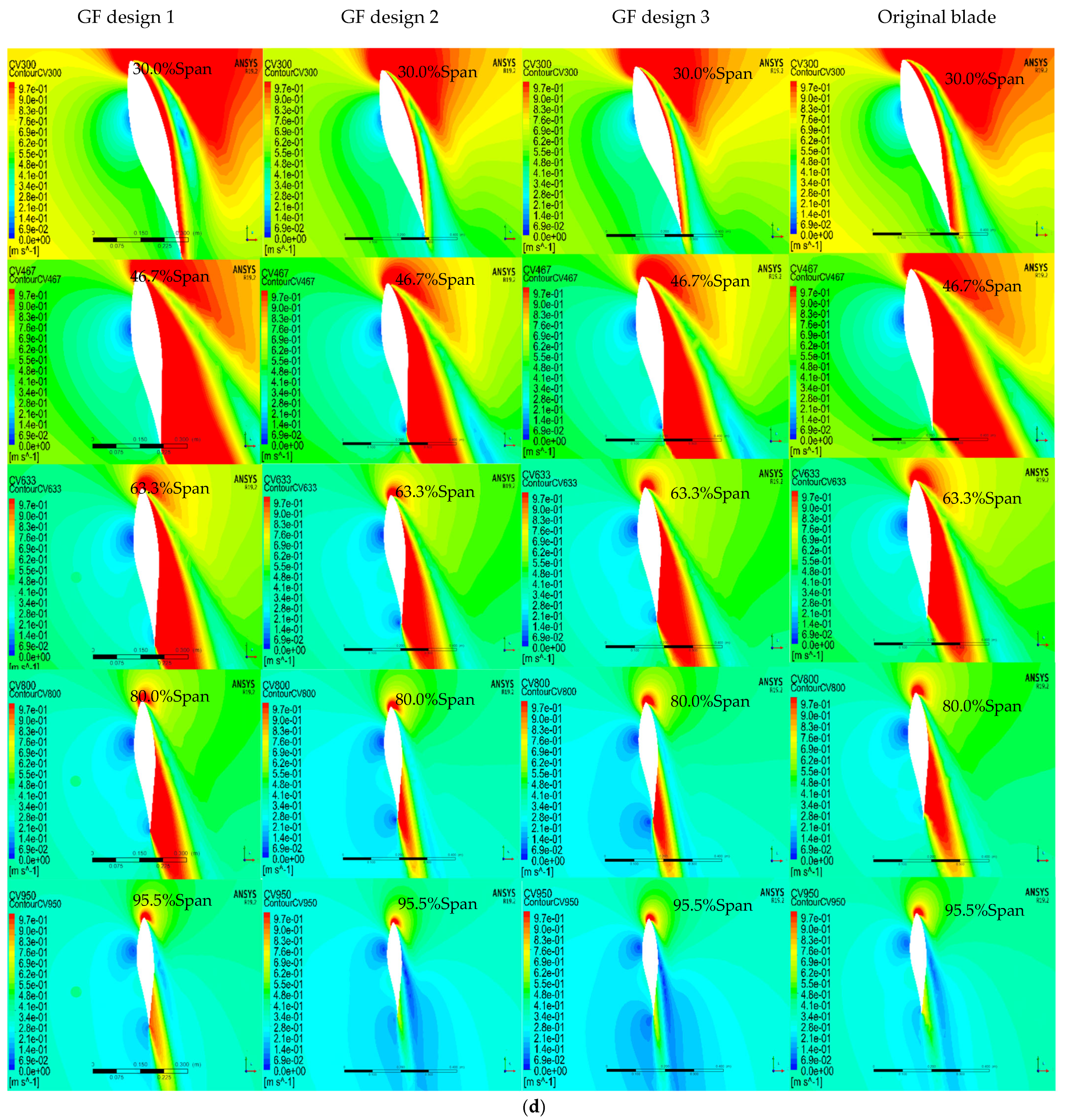
Figure 15d shows the velocity contour plots at a wind speed of 13 m/s. About 73% of the blade span from the hub stays in the deep stall region, and the rest of the blade remains in the dynamic stall region. Therefore, there are some variations observed in the contour plots. GF design 1 is marked for all span sections to show more flow separation compared to the original blade. The plot also shows that both GF design 2 and GF design 3 have less flow separation than the actual blade.

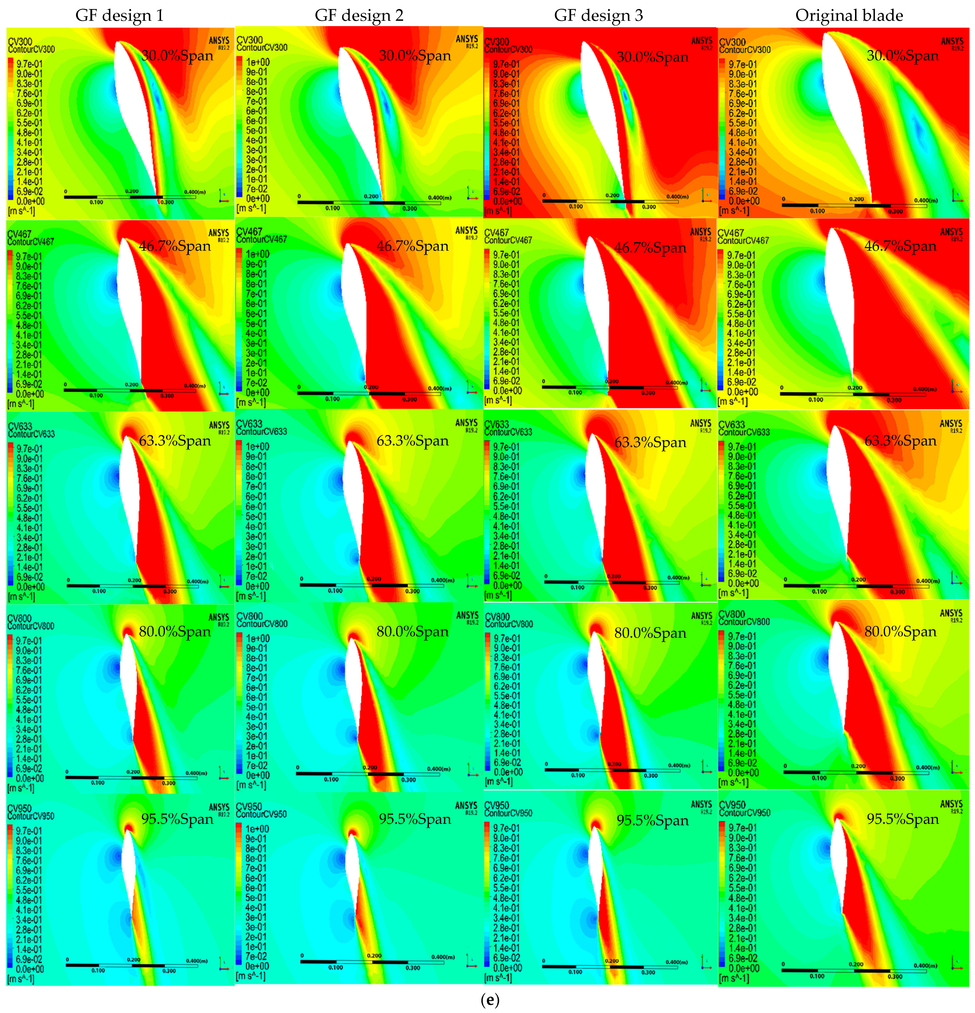
At wind speed, 15 m/s, about 90% of the blade span stays in the deep stall region, and the rest of the span remains at a dynamic stall region. At 30% and 46.7% of blade span sections, more flow separation is observed for GFs design 3 followed by the original than the GFs design 1 and 2. At 63.3%, 80%, and 95.5% blade span sections, Figure 15e shows that the original blade experiences the most flow separation followed by GF design 3 and GF design 1, respectively.

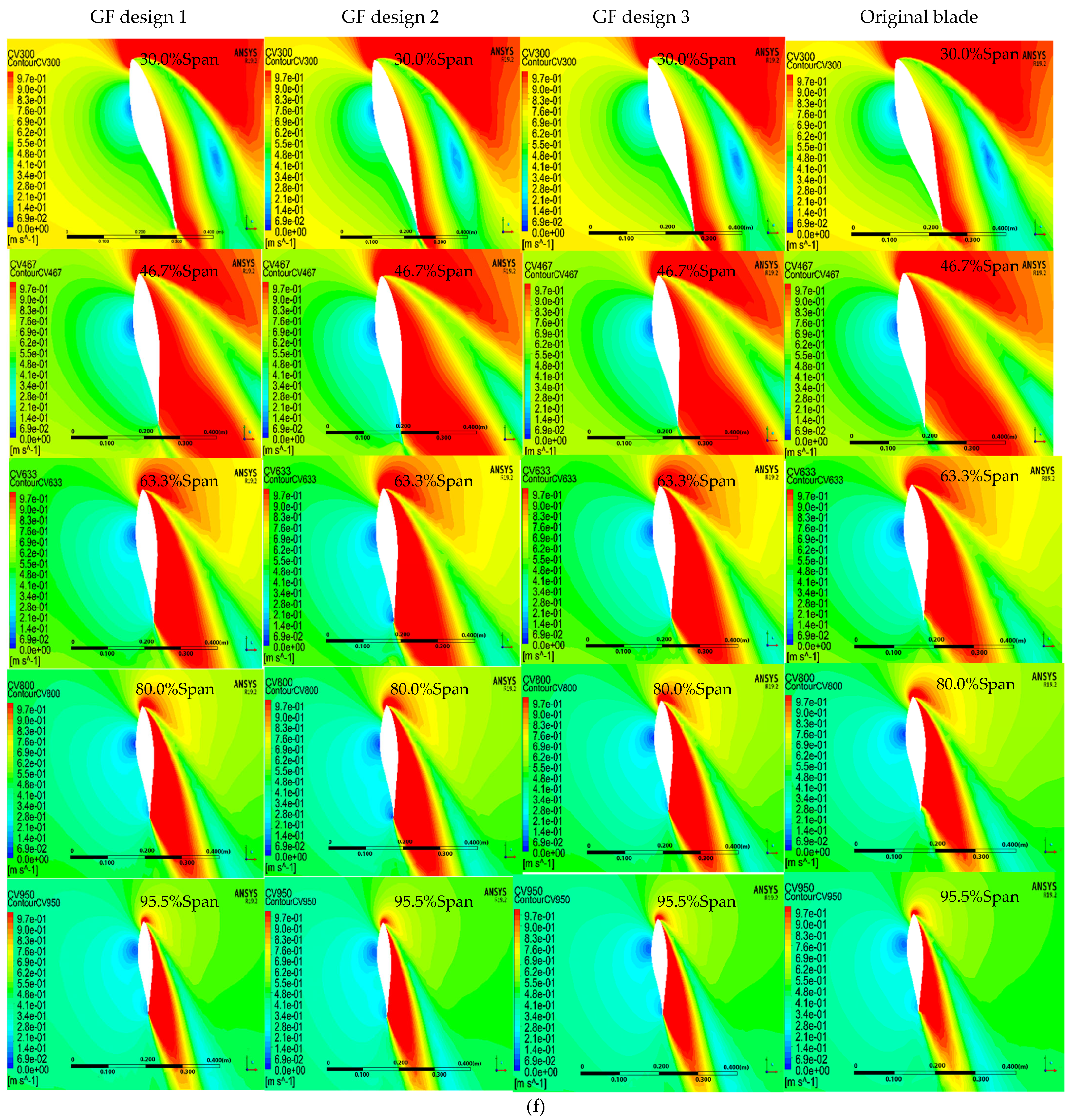
At a wind speed of 20 m/s, Figure 15f, the entire blade span remains within the deep stall region, and flow is fully separated from the hub to the rest of the blade. All sections for all four blades are almost identical. So, no effect of the addition of GF is observed for high wind speed.

The whole blade span remains within the deep stall region, and flow is fully separated from hub to tip. Therefore, less discrepancy is expected from all CP distribution curves at 20 m/s. Figure 15c shows the CP distribution curve for three GF cases, the original blade and the blade with a winglet. At a 30% span ratio, there was an under-predicted GF design 3 with the original NREL blade design. Both 30% and 40% span ratio predict the almost similar value at 20 m/s wind speed. For all sections of the blade span at 20 m/s, the CP distribution curve shows the same Cp value for all designs. However, all GFs designs have more positive Cp value at the trailing edge compared to the original blade and blade with a winglet.

The simulation results are used to compare the velocity contour coefficient for original blades with different GF heights at seven wind speeds and five blade span sections to validate the findings’ pressure coefficient contour.

4.3. Tangential Force Coefficient and Normal Force Coefficient

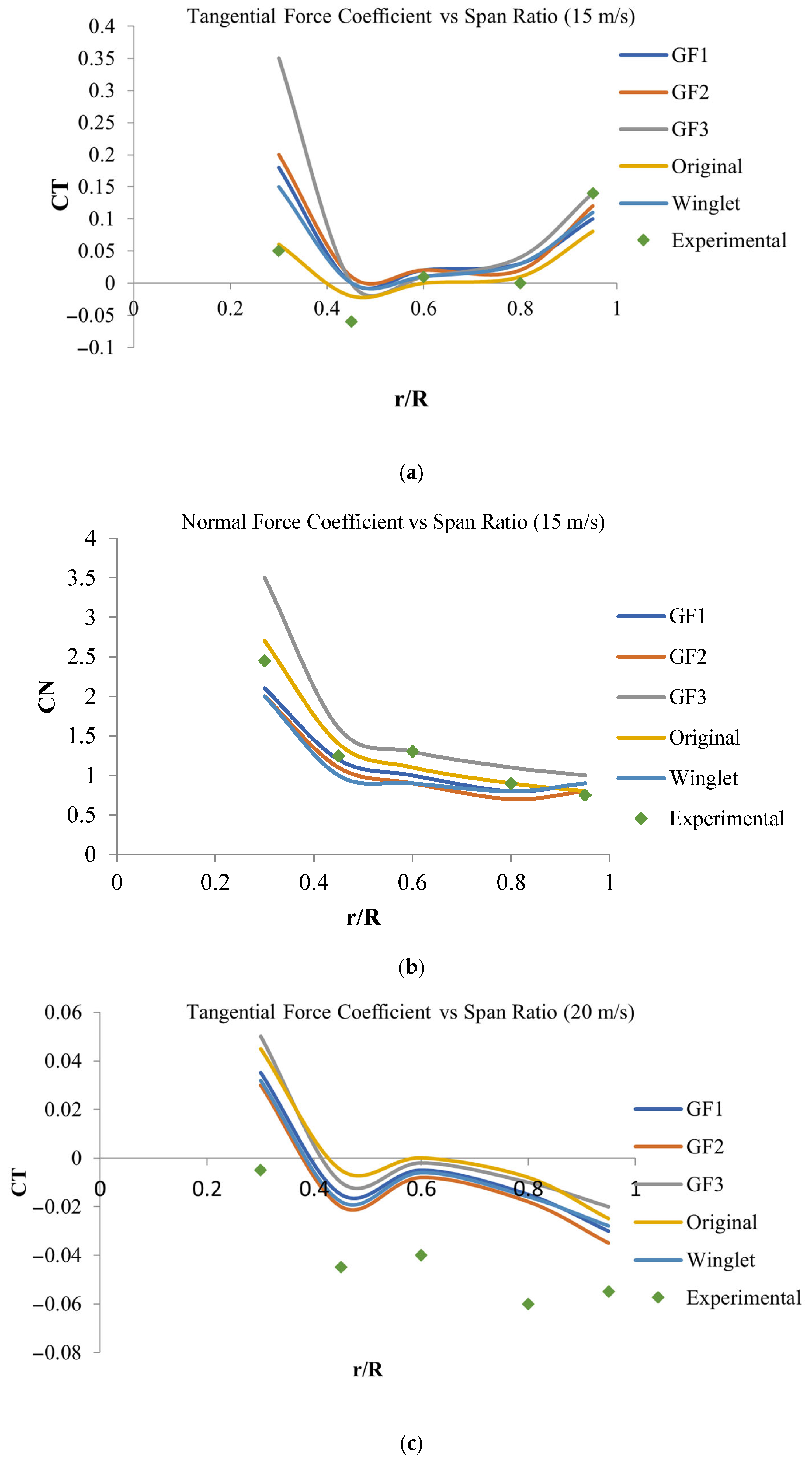
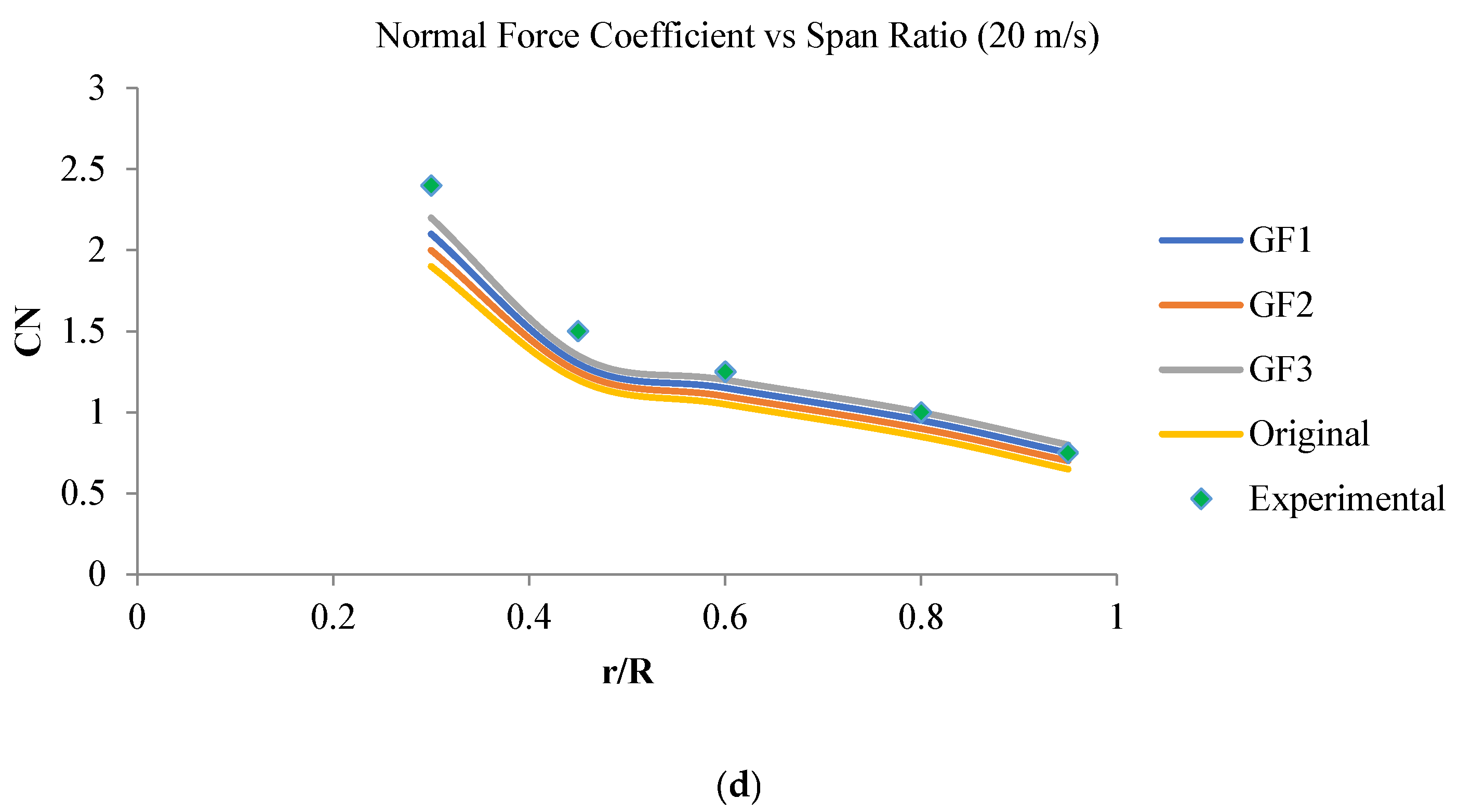
In this section, the normal force coefficient and tangential force coefficient distribution at different wind speeds (5 m/s to 20 m/s) along the span of a blade are demonstrated and explained. The curves are compared with all five blade designs under study. Tangential force is considered to be the force that acts tangent to a moving body’s path and is responsible for an increase or decrease in velocity. The force that acts perpendicular to the tangential force is known as the normal force, which influences motion direction without altering the speed. The (CT) and (CN) are non-dimensional parameters, making the comparison easier. CT acts parallel to the chord line, and CN acts perpendicular to the chord line.

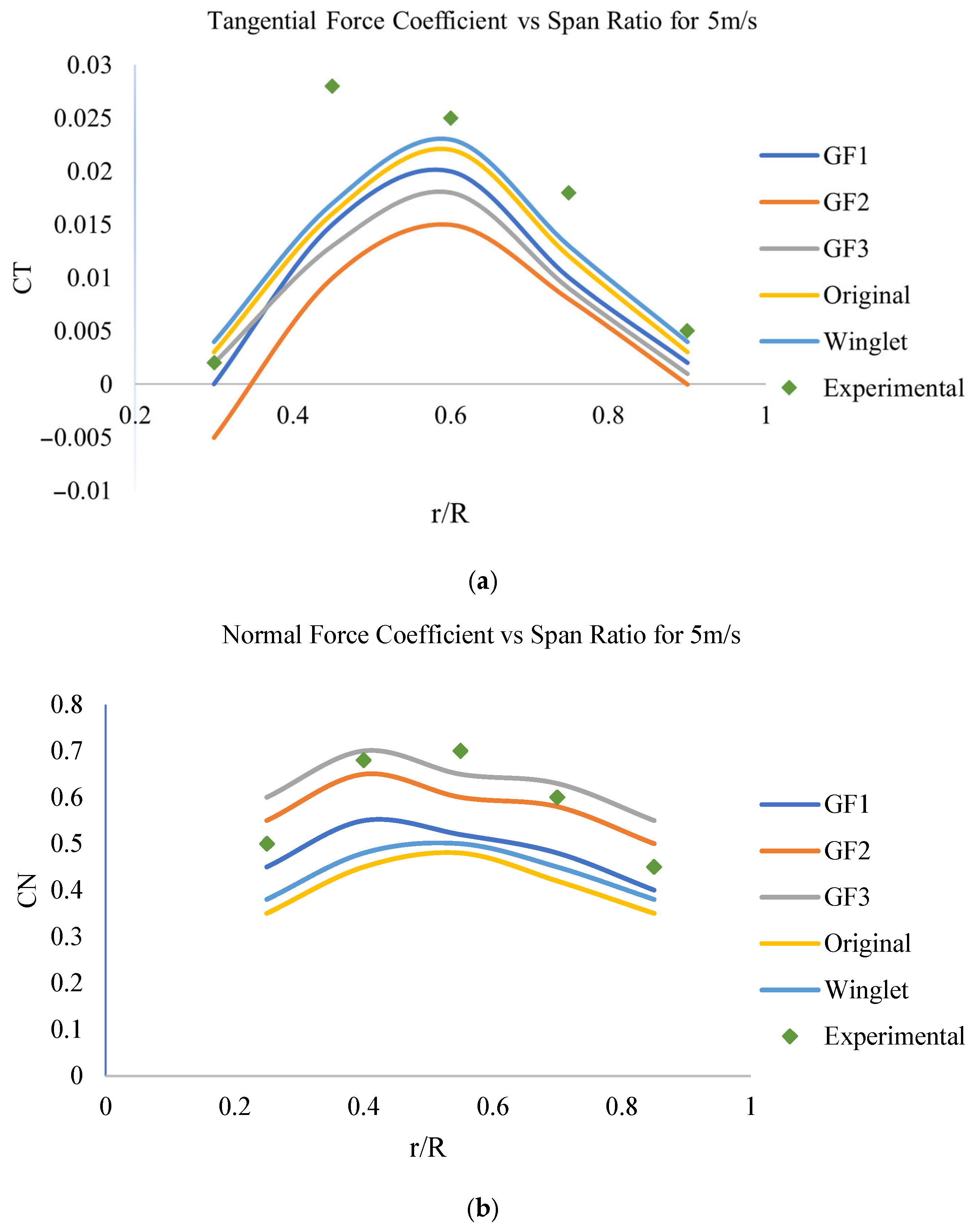
At a wind speed of 5 m/s, as shown in Figure 16, the (CT) distribution along the span for all the blade designs since the entire blade span stays in the attached flow region. And AoA range is minimal; an insignificant difference in (CT) distribution is observed at this wind speed. The (CT) values varied from around 0.01 at the hub to a maximum amount of about 0.02 at mid-span and then decreased to the tip. On the other hand, a more considerable variation is observed by (CN). The highest values are observed for GF design 3, followed by GF design 2. The difference between the other blades was minimal. The highest value for GF design 3 was about 0.7 at around mid-span. 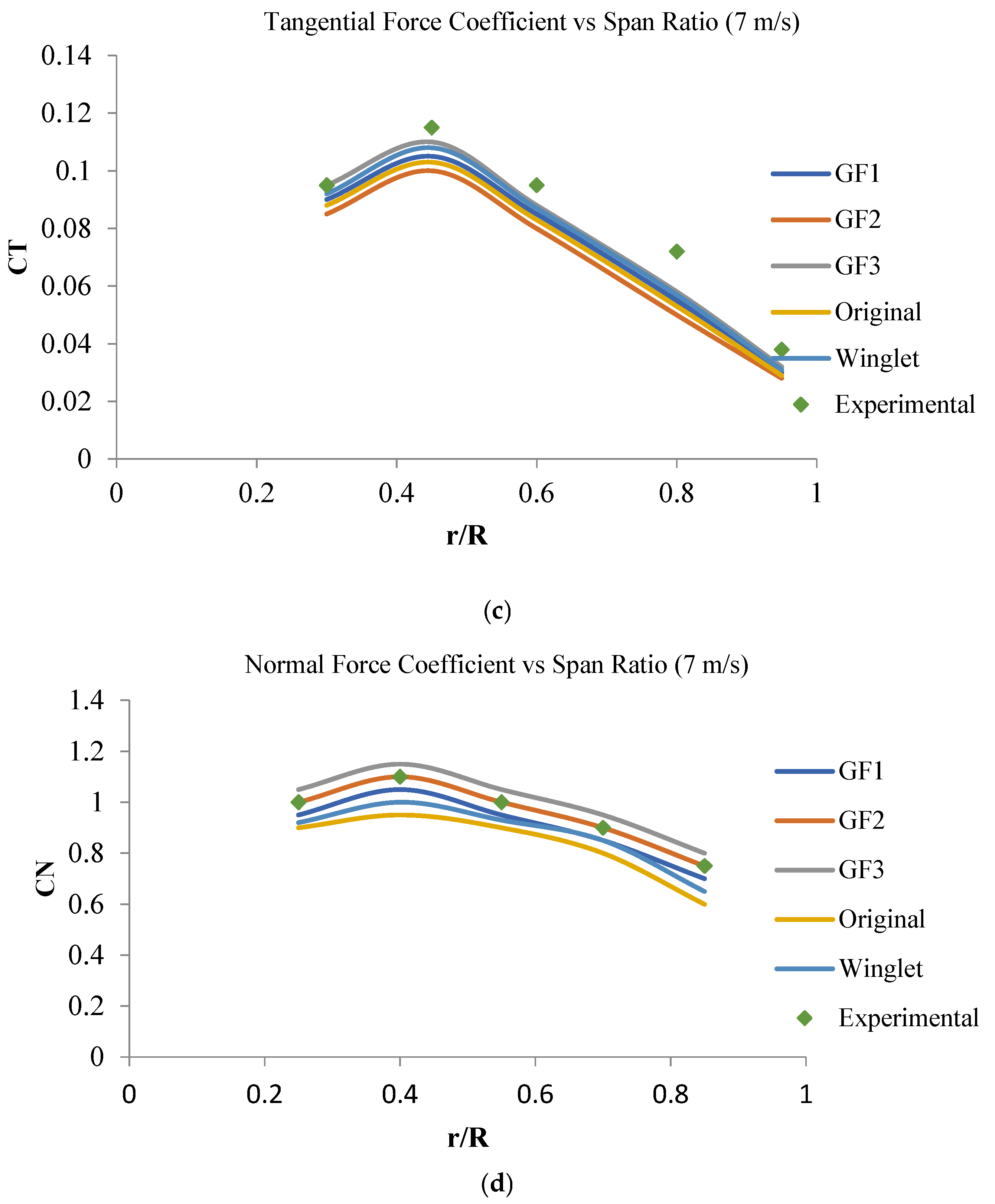Figure 16 shows the (CN) and (CT) distribution at 7 m/s wind speeds along the span. At this speed, the entire blade is in pre-stall region. The difference between various designs is almost like that of 5 m/s. The location of the highest values shifted closer to the hub to around 45% span location. The (CT) variation along the blade span is almost the same for all blade designs. The (CT) values increased from around 0.09 near the hub to approximately 45% span location and then gradually reduced to about 0.03 at the tip. The highest value of (CN) was observed by GF design 1, where the value is 1.1 at a 45% span to about 0.7 at the tip. The values of (CN) for GF design 2 are a little less than GF design 3 followed by GF design 1, design with winglet, and original blade.

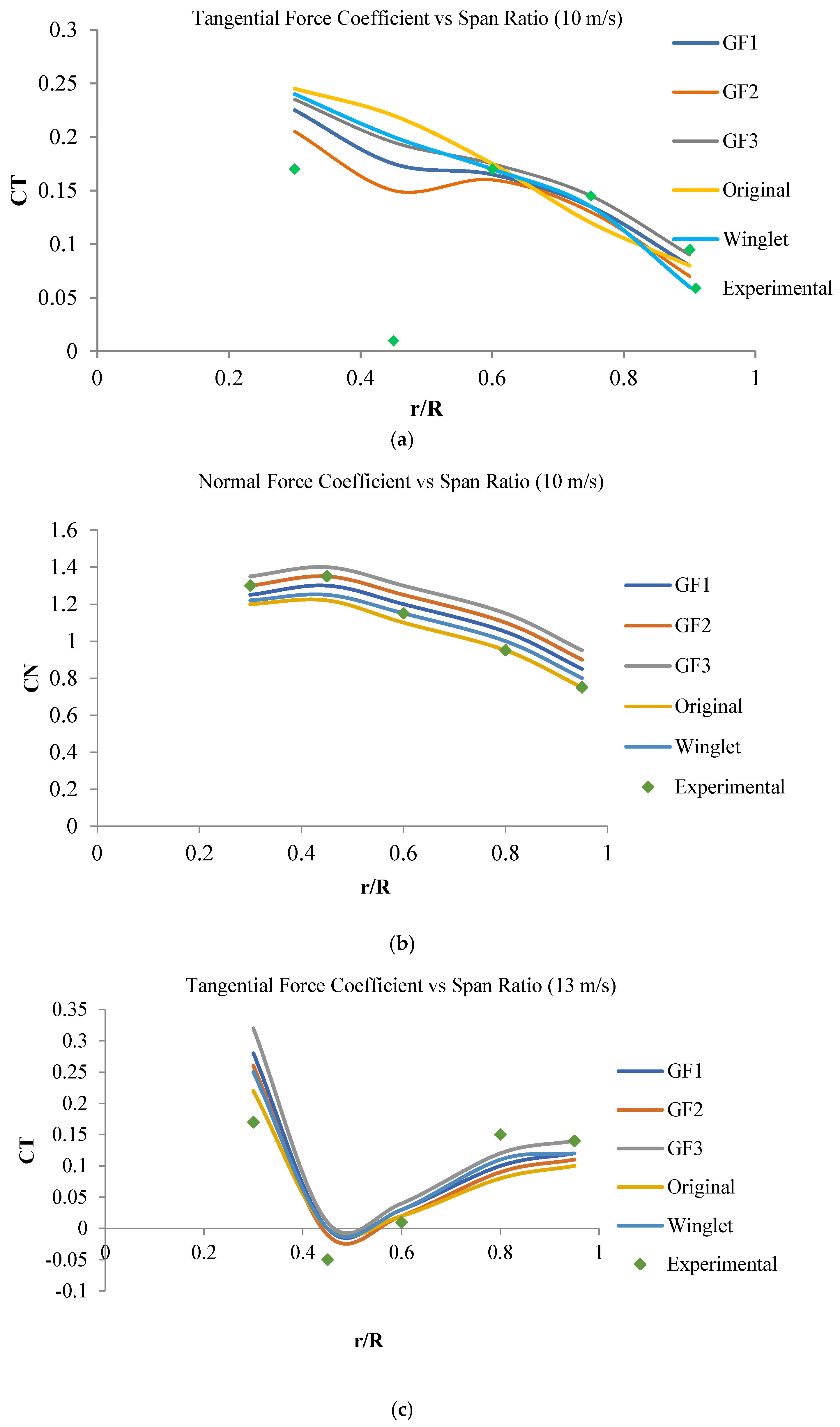
At 10 m/s wind speed, both (CT) and (CN)’s maximum values moved to the blade section nearest to the hub and continuously decreased towards the tip. Figure 17 shows up to 46.7% at this wind speed, the blade span section is in the deep stall region, 46.7% to 73% of the span is in the dynamic stall region, and the rest of the blade span is in the pre-stall area. The (CN) value for a couple of designs, GF designs 1 and 3, the (CN) starts to increase from 70% span to a maximum amount at 80% span before starting to decrease again. The highest (CT) values of about 0.25 were observed for original blade shape and design with winglet, and for (CN) it was a value of 1.5 for GF design 3. 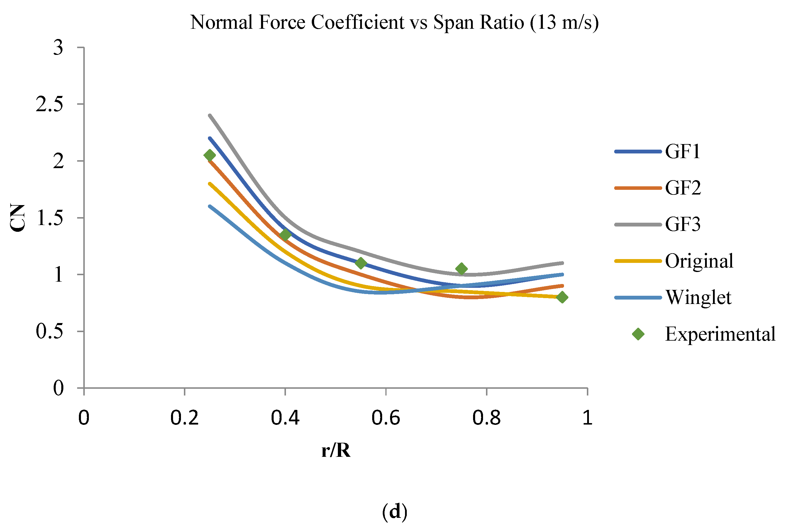Figure 17 also shows the (CT) and CN distribution curve of the blade with GF cases, original NREL Phase VI, and blade with a winglet results at 13 m/s wind speed. Around 73% of the blade span from the tip stays in the deep stall region, and the remaining part of the blade remains in the dynamic stall region. The separation between the deep stall region and dynamic stall region takes place at 200 AoA. Therefore, a higher force value is expected. The highest amount of (CN) is observed by GF design 1 up to 45% span blade. From the 45% to 55% span, the FG design 2 and design 3 donate the highest CN value, and from about 80% of span up to 100% GF, design 3 shows the highest amount of (CN) as well as a blade with a winglet. The (CT) curve shows that about up to 50% of span GF design 3 is observed as the highest value of (CT). From about 55% of span up to the rest of span, the original blade gains higher (CT) value than the others, followed by GF design 3.

Figure 18 shows (CT) and (CN) for Gurney flap designs, original NERL blade, and blade with a winglet at 15 m/s wind speed. Approximately 90% of the blade span from the hub stays in the deep stall region, and the rest of the span remains at a dynamic stall region at this wind speed. It also faces the onset of full separation of 20° AoA at a 90% span location. Therefore, the (CT) is expected to rise after the 20° AoA. Up to about 45% of span, all the Gurney flap designs have higher (CT) value compared with original NERL. Among the three GF designs, GF design 3 shows the highest (CT) value, followed by GF design 1. From 63% to the rest of the blade span, the GF design 1 shows the highest (CT) value and the winglet blade. Moving on to the (CN), Gurney flap design 3 offers higher value than all blades’ design for all span sections. GF design 1 and design 2 are observed to have higher (CN) values than the blade with winglet and lower CN value than the original blade. Figure 18 shows the (CT) and the normal force coefficient distribution curve for 20 m/s wind speed. At 20 m/s wind speed, the entire blade remains in the deep stall region. Therefore, the flow is entirely separated, and the (CT) distribution curve is expected to represent a lower value. The highest (CT) curve is donated by GF design 1 to 45% blade. Later, at 80% of the blade span, the blade with Gurney flap design 3 value becomes very similar to the original CFD phase. (CT) value of all designs of Gurney flap blades and blades with winglet were almost identical except for Gurney flap design 3, which exhibits a higher value than others.

All case blade designs in the (CT) are very similar to the original CFD blade and the entire blade span AoA remains in the deep stall region at this wind speed. So, the flow is entirely separated, and the (CT) is expected to be very low. All the designs with Gurney flaps and winglet exhibit almost the same result as the original blade result.

4.4. Torque

The torque force causes the blade’s rotation, which leads to the rotation of the shaft, which then causes the generator to engage and generate power. However, more torque will allow the wind turbine to produce more energy.

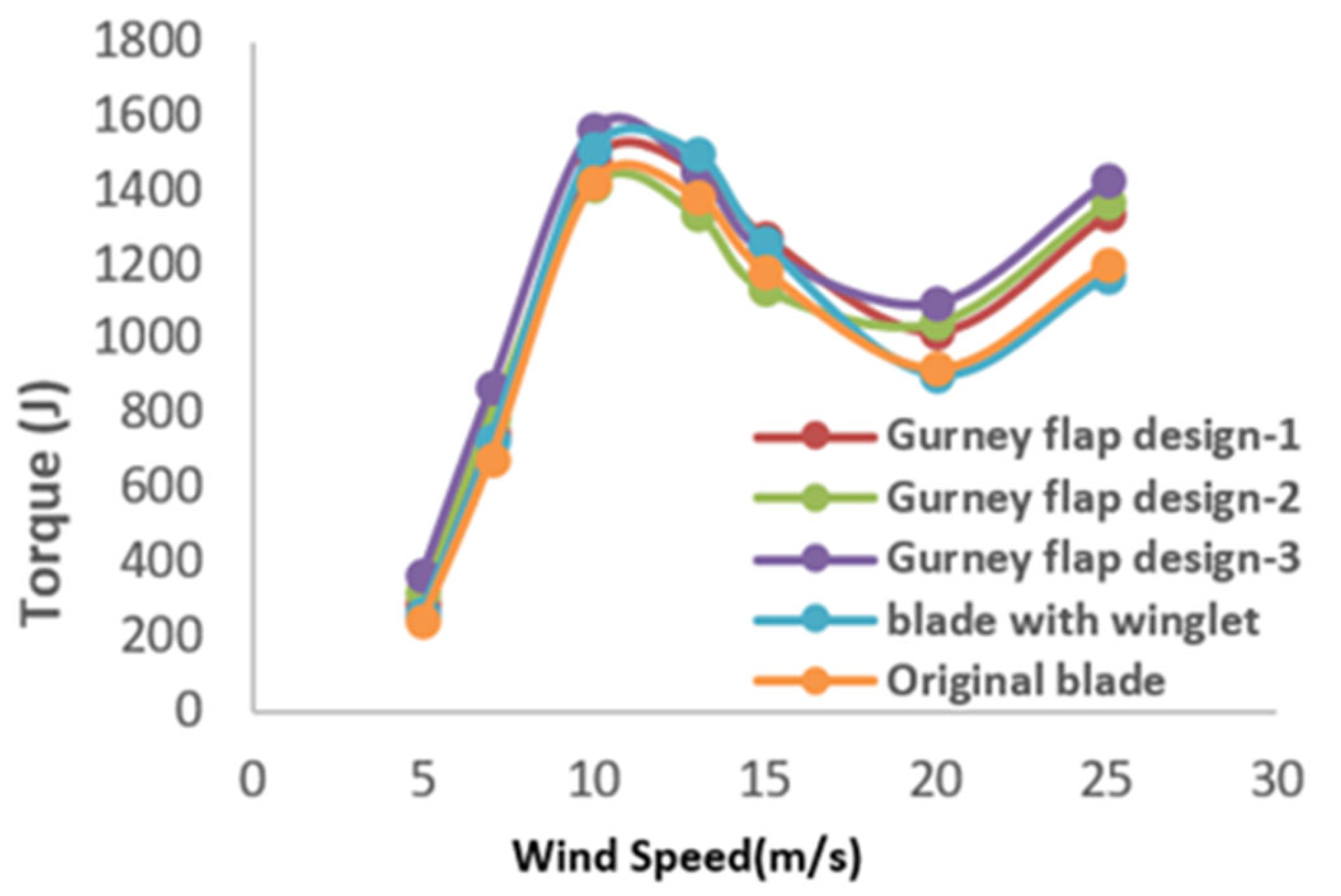
In this research, the torque result will be imported by ANSYS 19.2 simulation of three different wind blade designs with GFs using seven speeds to compare with the torque’s result of the original wind blade and original wind blade with a winglet, as shown in Figure 19.

At wind speed 5 m/s, the blade’s torque value with GF design 1 shows the same result of the original blade and blade with a winglet. That was because the GF’s length in design 1 is small, and the AoA is very small, so the entire blade stays in the attached region. Applying low wind speed will not show any difference in torque value for GF design 1. However, the blade with GF design 3 offers the higher torque value, followed by GF design 2. That is because the length of GFs design 2 and design 3 is higher than the blade with GFs in design 1.

At wind speed 7 m/s, the torque value of the blade with GF design 1 shows little more torque value than the torque value in the original blade and blade with winglet. On the other hand, the blade with GF design 1 gives a torque value less than the blade’s torque value with GFs design 2 and 3. Therefore, higher power is expected from blades with GFs.

At wind speed 10 m/s, the blade’s torque value with GFs design 1 shows more than the original blade and almost the same as the blade with a winglet. The torque value of blade with GF design 3 offers the highest torque value of all designs. Thus, higher power is expected from blades with GF design 3.

At wind speed 13 m/s, the blade’s torque value with GFs design 1 and 3 shows more than the original blade and less than a blade with a winglet. However, the blade with GF design 2 offers less amount of torque. As a result, higher power than the original blade is expected from blades with GFs 1 and 3; however, a blade with a winglet can produce more power than the rest of the designs.

At wind speed 15 m/s, the torque value of blade with GF design 1 shows the highest amount of torque value, which will lead to the highest power of all other cases. A blade with GF design 3 gains more torque value than the original blade and almost the same value as a blade with a winglet. In general, the blade with GF design 1 and design 3 can have higher power than the original blade.

At 20 m/s wind speed, the flow is fully separated. The torque for all three blades with GF cases shows more value than the original blade and blade with a winglet. However, three GF cases have different torque values compared to each other. GF design 3 delivers the highest torque compared to GFs design 1 and 2, and GFs design 2 offers torque value in GFs design 1 and 3. As a benefit of this wind speed experiment, higher power is expected from all blades with GFs.

The addition of GFs has shown the beneficiary effect for high wind speed. Finally, more torque value leads to more power, which is expected from all blades with GFs.

In addition to torque and thrust, the power coefficient ($C_p$) was evaluated to provide a normalized measure of the aerodynamic performance of the different blade configurations. The power coefficient was calculated using the predicted aerodynamic torque and rotational speed, allowing a direct comparison of power extraction efficiency under varying wind speeds. The trends observed in $C_p$ are consistent with the torque results, with the Gurney flap-modified blade showing improved performance at medium to high wind speeds, while differences remain small at lower wind speeds.

The power coefficient is defined as

$$C_p={\displaystyle \frac{T\hspace{0.17em}\omega }{\frac{1}{2}\rho A{V}^3}}$$

where $T$ is the aerodynamic torque, $\omega$ is the angular velocity of the rotor, $\rho$ is the air density, $A$ is the rotor swept area, and $V$ is the free-stream wind velocity.

4.5. Thrust Force

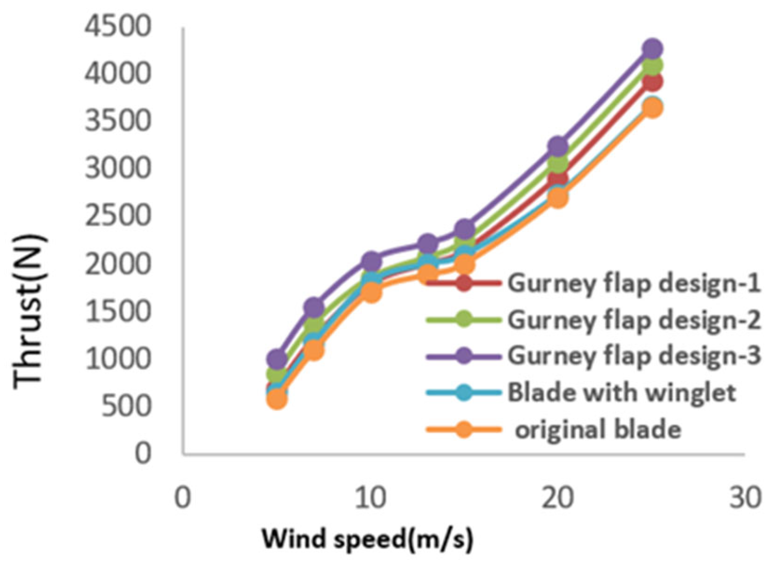
Normally, the thrust force of an object is related to the surrounding flow characterized by the momentum theory Thrust could have some negative effect on the stability of a wind turbine at the same wind speed. Consequently, this will lead to the loss of some of the wind energy. Therefore, a higher value of thrust caused a worse effect on the wind turbine’s efficiency. The results for the thrust of seven wind speeds applied on blades with GFs, original NERL blade, and a blade with a winglet are obtained from CFD simulation, as presented in Figure 20. The wind speed experiment at 5 m/s showed that the thrust force for GF design 1 was almost like the thrust force of the original wind turbine and blade with winglet, leading to the same stability. However, it shows a higher thrust force on GFs design 2 and 3 than all other designs, which might affect the wind turbine’s stability.

At wind speed, 7 m/s, the wind turbine blades’ stability has stayed almost the same for GFs design 1, original blade, and blade with winglet because thrust remains nearly the same for all three cases. GFs design 2 and 3 show less stability than all three instances above on wind turbine blade based on higher thrust force generated by wind speed.

At 10 m/s wind speed, thrust force for GF design 3 is shown as the highest value compared to all cases. GFs design 1 and design 2 have almost the same thrust force value as the blade with winglet and more thrust force than the original blade. Therefore, there is almost less stability on wind turbine structure among all three GF cases expected from GFs design 3.

Also, the thrust force observed from 13 m/s wind speed remained the same as the variation in thrust force for all cases as the results obtained from the experiment in the wind speed 10 m/s. Thus, the wind turbine blades’ stability with GF design 1 remains the same as the blade with a winglet and original blade.

At 15 m/s wind speed, thrust force results of GFs design 2 and 3 are high compared to CFD results of GFs design 1, original wind blade, and blade with winglet. On the other hand, the CFD result of GFs design 1 shows a higher thrust force than the original wing blade and almost the same thrust force as a blade with a winglet. Thus, the stability of the wind blade with GF design 1 is expected to be the same as the blade with a winglet and original blade. Among three GFs cases, the blade with GF design 1 shows the best stability.

At 20 m/s wind speed, the flow is fully separated after passing on the blade surface. CFD simulation of three GF designs shows higher thrust force results than the original wind blade and the blade with a winglet. However, for all three blades with GF cases, comparatively lower thrust value is observed by the blade with GF design 1. High wind speed shows the blade has less stability with GFs compared to the original wind blade and blades with a winglet.

5. Conclusions and Future Work

5.1. Conclusions

This study numerically investigated the aerodynamic performance of the NREL Phase VI wind turbine blade after adding Gurney flaps. Three different Gurney flap heights were applied at the trailing edge. The results indicate that the presence of Gurney flaps improves torque and power output over a wide range of wind speeds when compared with the original blade and the blade equipped with a winglet.

At low and moderate wind speeds (5–10 m/s), the larger Gurney flaps (GF design 2 and GF design 3) produced higher torque. This improvement is associated with increased pressure difference and delayed flow separation at the trailing edge. At higher wind speeds (13–15 m/s), the performance became sensitive to flap height, and excessively large flaps led to local flow separation and reduced efficiency. Under separated flow conditions at 20 m/s, all Gurney flap designs generated higher torque than the baseline blade; however, GF design 3 provided the best overall performance.

These trends are consistent with three-dimensional flow mechanisms, indicating that trailing edge and blade-tip modifications influence vortex formation, wake interaction, and power coefficient. In addition, the small change observed in the normal force suggests that the proposed designs do not significantly increase structural loading on the turbine [23].

Overall, the results verify that Gurney flaps can be an effective passive method. It helps improve wind turbine performance, with GF design 3 (2% chord height) providing the most consistent enhancement within the tested wind speeds.

5.2. Future Work

Based on the literature review and research, the following studies are recommended for further analysis. Implementing different parameters of GF can be modified to study the variation in the aerodynamic effect. Considering different methods are needed to obtain the optimal shape of the Gurney flaps. Structural analysis of the wind turbine blades equipped with GF should be conducted using FSI (fluid–structure interaction) to study the blade’s stability. Adding the GF could be used for offshore wind turbine blades. Furthermore, conducting noise analysis and noise reduction for the blade with a winglet could be investigated in the future.