A Support Process for Early-Stage Wind Farm Repowering Decisions Using Constrained Optimization Techniques to Address Uncertainty

Abstract

As wind farms in North America near the end of their design life, different end-of-life options need to be considered. Common options include decommissioning, lifetime extension, and repowering. In this research, a methodology to support early-stage repowering decisions is presented. Performance decline and repowering forecasts are obtained by combining analysis of past performance data and preliminary site plans for new turbines with turbine performance models from windPRO software. Financial metrics are computed using a simple techno-economic model with parameters informed by historical financial records. Repowering decisions are often sensitive to assumptions on key parameters, such as capital cost of repowering, which are poorly defined at the beginning of the process and subject to change quickly. This makes it difficult to provide guidance that will remain relevant as more information is obtained during future project planning stages. In this work, constrained optimization methods are used to identify sets of the key inputs that lie on the break-even point at which repowering is more profitable than continuing operation. Using this approach, which is novel in this context, the client gains an intuition for the ‘envelope’ within which the recommended guidance still holds. This decision-making process is applied to a case study using performance data and cost ranges from a real, anonymous wind farm.

1. Introduction

As the onshore wind energy sector continues to mature, numerous wind farms are approaching end of life; to give a sense of scale, Wood Mackenzie forecast that 275 GW of onshore wind power would reach 20 years of operations between 2023 and 2033 [1]. The owners and operators of these farms are faced with a variety of end-of-life options. They may simply run the wind farm to failure, leaving all turbines working with minimum maintenance until maintenance costs are higher than revenues or it is unsafe to continue, and then decommission the wind farm completely. Another possibility is lifetime extension, in which the farm continues running past the design life with only minor replacements or upgrades. Lifetime extension may be supported by assessments of structural integrity and remaining useful life of components (e.g., [2]), or operational changes to reduce stress on aging components during an extended lifetime (e.g., [3]). Alternatively, partial repowering refers to a greater investment where significant components within the turbines are replaced, typically aiming to both extend operating life and increase energy production. For example, GE offers enhancements for some of their older turbines by replacing the drivetrain, rotors, and controls technology with upgraded components [4]. Partial repowering is also sometimes used to refer to situations where some turbines are replaced while others are left standing [5].

By contrast, Full Repowering entails a replacement of all the turbines. A significant driver for repowering is to increase the energy yield per unit area, and results have consistently demonstrated an increase in annual energy production [6,7,8]. Full repowering projects still offer substantial advantages over greenfield developments. They can leverage existing infrastructure such as cables and substations to save costs and reduce environmental impacts. Since wind as a resource is already well understood, there can be a reduction in project risk and improved financing conditions. However, changes in regulations and social acceptance may impose new constraints which reduce operating capacity [9]. Wind farms may ultimately use a combination of the approaches above, such as a lifetime extension for a certain number of years followed by a full repower. Studies have shown that the most appropriate end-of-life strategy depends heavily on site-specific factors such as the operational expenditure and electricity yield of the old turbines, as well as the development of electricity prices [3,5,8,10,11]. For example, when Piel et al. applied the selection and design of optimal end-of funding strategies to 1645 turbines in the aging German wind fleet, they recommended immediate repowering for 33%, continued operation followed by repowering for 28.5%, lifetime extension without subsequent repowering for 17%, and no further investment for 21.5% [3]. Therefore, decision-support processes are needed to help the owners and operators of aging wind farms select the most suitable options for them.

Decision-support tools for end-of-life options for individual wind farms typically focus on computing the financial return on investment for each option using the net present value (NPV), levelized cost of energy (LCOE), or internal rate of return (IRR) [7,8,11,12,13]. Notable exceptions include the works of Bezbradica et al., who use multi-criteria decision analysis involving multiple stakeholders [14], and Safaei et al. who employ multi-criteria optimization [15]. The improvements in energy yield that can be gained from repowering have been estimated using numerical analysis from historical wind farm projects [6,7] applying power curves to wind speed frequencies [8,16], or using wind power assessment tools such as WAsP which account for wake losses and site-specific physical characteristics [5,17,18]. More detailed approaches to estimating annual energy production also exist, primarily relying on computational fluid dynamics [19,20,21]. Notably, previous works diverge considerably in their reporting of the impact of key uncertainties on end-of-life decisions. A sensitivity analysis is sometimes reported [8,22]. Leite et al. extend this approach by including a Sobol sensitivity analysis to identify critical variables [10]. Villena-Ruiz et al. reported on the minimum spot price needed for profitable repowering [8], while Jadali et al. computed the certainty equivalent of LCOE [23]. Ramirez et al. perform Monte Carlo analysis [22] and Madlener et al. employed a real options approach [24].

While sensitivity analysis is useful to identify individual inputs for which uncertainties are most impactful, it does not provide information about how much inputs can change individually or in combination before a different decision would be recommended. When the degree of uncertainty is well-quantified, statistical methods such as Monte Carlo and real options analyses can provide the best choices in the face of that uncertainty. However, when the uncertainty is not well-characterized and assumptions about key inputs are subject to change quickly, guidance from those types of analyses can soon become outdated. Specifically, Monte Carlo provides the statistical distribution of an output (such as NPV of a repowered plant) resulting from the combined result of the assumed uncertainties in all the inputs (e.g., operations and maintenance expenses, capital expenditure of repowered plant, discount rate). However, the effect of any single input on that distribution is not distinguished. If updated information changes the value or uncertainty for an input, then there is no way to infer how this may change the distribution and recommendation without re-computing. The real options approach does consider a set of possible options and has internal logic for when each option is taken. The internal logic is typically based on an intermediate project value metric (e.g., deciding to act when the NPV of an action is greater than the value of waiting). However, the primary focus of the real options approach is in computing the expected net present value of an option, assuming that the operator will exercise that option intelligently across time, rather than describing relationships between input and outputs. Again, generally if the understanding of the input values are updated then the analysis will need to be re-computed (there could be exceptions in which detailed descriptions of the input conditions where each option is exercised are presented).

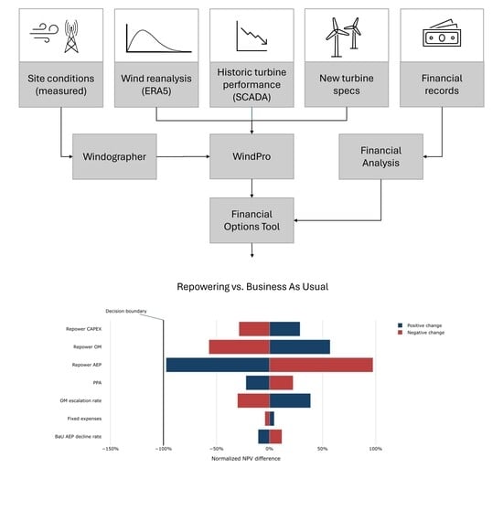
Repowering projects typically undergo multiple decision-making stages in which estimates for key inputs (e.g., capital cost of a future repowering project) are initially uncertain and become increasingly precise over time. The goal of this work is to provide decision makers with useful guidance at the beginning of this process. This method seeks to identify the best early-stage options (continue operating, partial repower, etc.) and quantify the degree to which key inputs, individually and in combination, can differ from the original assumptions before the recommended option changes. The hope is that this will allow decision makers to set off on a good path and, as planning progresses, gauge whether the new information they are receiving at later stages may require them to re-consider their current path. To do this, we combine analysis of turbine SCADA data and financial records with windPRO modeling to estimate performance decline for the current farm, then predict energy yields from realistic topologies with new turbines that are currently on the market. A simplified financial model identifies the approaches with the highest predicted net present value. We then employ constraint-based optimization methods to search for combinations of inputs at the ‘decision boundaries’ between the repowering options that seem most applicable.

To our best knowledge, this decision-support framework is novel within the context of repowering decisions as follows:

• This framework responds to uncertainties by presenting clients with multiple sets of input parameters that exist on the boundary between the top two decisions that could be made (repower vs. continue to operate as usual, full repower vs. partial repower, etc.).
• The sets of input parameters are selected by solving constrained optimization problems in which the objective function penalizes moving input parameters away from their expected value.
• Different penalty functions are used to select different sets of decision boundary inputs, reflecting subjective preferences for which sets of input parameters may be most practically useful to the client.

The full sequence of approaches used within this framework has not been reported previously in the repowering decision support literature.

This approach has multiple advantages:

• It supports a conceptual understanding of risks and their underlying causes at a time when estimating future uncertainty with past statistics is potentially misleading (e.g., turbine performance decline is expected to accelerate towards end of life, limiting the predictive value of past performance).
• Accounting for interactions between parameters, it provides more detail about which combinations of input parameters may change the recommendation, allowing early monitoring and more detailed analysis for those parameters.
• When the expected value of an input parameter changes, the client may still be able to interpret what their best choice is without re-computing.

The decision-making process is applied to a case study using performance data and cost ranges from a real, anonymous wind farm.

2. Materials and Methods

2.1. Past Performance

Measured wind speed, wind direction, and temperature data from the period 2018–2024 was obtained from a nearby met mast. Windographer was used to remove unrealistic values and data from time periods when sensors that were at the same height substantially disagreed, since this often indicates icing conditions or other irregularities. A representation of the site was created in windPro, which accounted for surface roughness, obstacles, other turbines, and other physical factors at the site. Roughness lines were drawn manually, with terrain informed by windPRO 2022 Global Satellite Imagery. A sensitivity analysis found that model results were not very sensitive to the assigned roughness lengths, probably because the met mast was fairly close to the turbines. Using windPRO’s PARK module with the WAsP library [25], a time-varying analysis based on measured data was performed. This yielded a time series with predicted wind speed and power output for each turbine’s location within the current farm at 10 min resolution. The Jensen Park 2 wake model was used with a 0.90 wake decay constant. This location is a complex coastal location, with the met mast and all turbines within 1 km from the shoreline, sometimes in multiple directions. A 5% post-correction, tuned by SCADA performance data, was applied to the measurement mast scaler for 5/16 directional sectors to help account for this issue. While this case study focuses on repowering analysis for a particular area with only one type of turbines, there were multiple types of turbines at different hub heights across the site, and their SCADA data was used to ensure that post-correction did not over-fit at a particular hub height or set of turbines.

The wind speed and turbine power output estimates were compared with the measured values from SCADA data on four of the turbines for a time period of at least 3 years; the length of data provided by the client varied slightly between turbines, and the data for only four turbines were provided. Periods of curtailment were excluded (filtered out in Windographer as unreasonable values in a scatter plot of power vs. wind speed), as were periods of icing (identified in Windographer when cold conditions were found in conjunction with increasing disagreement between met mast measurements and eventually power vs. wind measurements). One period of extreme weather was also filtered entirely, because there were grid outages as well extended turbine downtime resulting in time steps becoming visibly out of sync for some of the measurement instruments. The mean bias error, root mean square error, and cross-correlation coefficient were computed for each turbine.

Windographer’s pattern recognition and Markov-based data reconstruction functions were then used to fill any data gaps in the meteorological time series (this represented less than 5% of the time series). A time-varying PARK analysis was conducted using the same model described above to obtain an annual sum of modeled energy production $G_y$ for each year y between 2018 and 2023. $\overline{G}$, an estimate of the mean annual production at the site, was also computed from a standard PARK analysis with WAsP. The WAsP statistic was exported from windPRO after using the Matrix MCP (Measure-Correlate-Predict) method with ERA5 wind speed at 100 m between 31 December 1978 and 15 January 2026 as a reference. 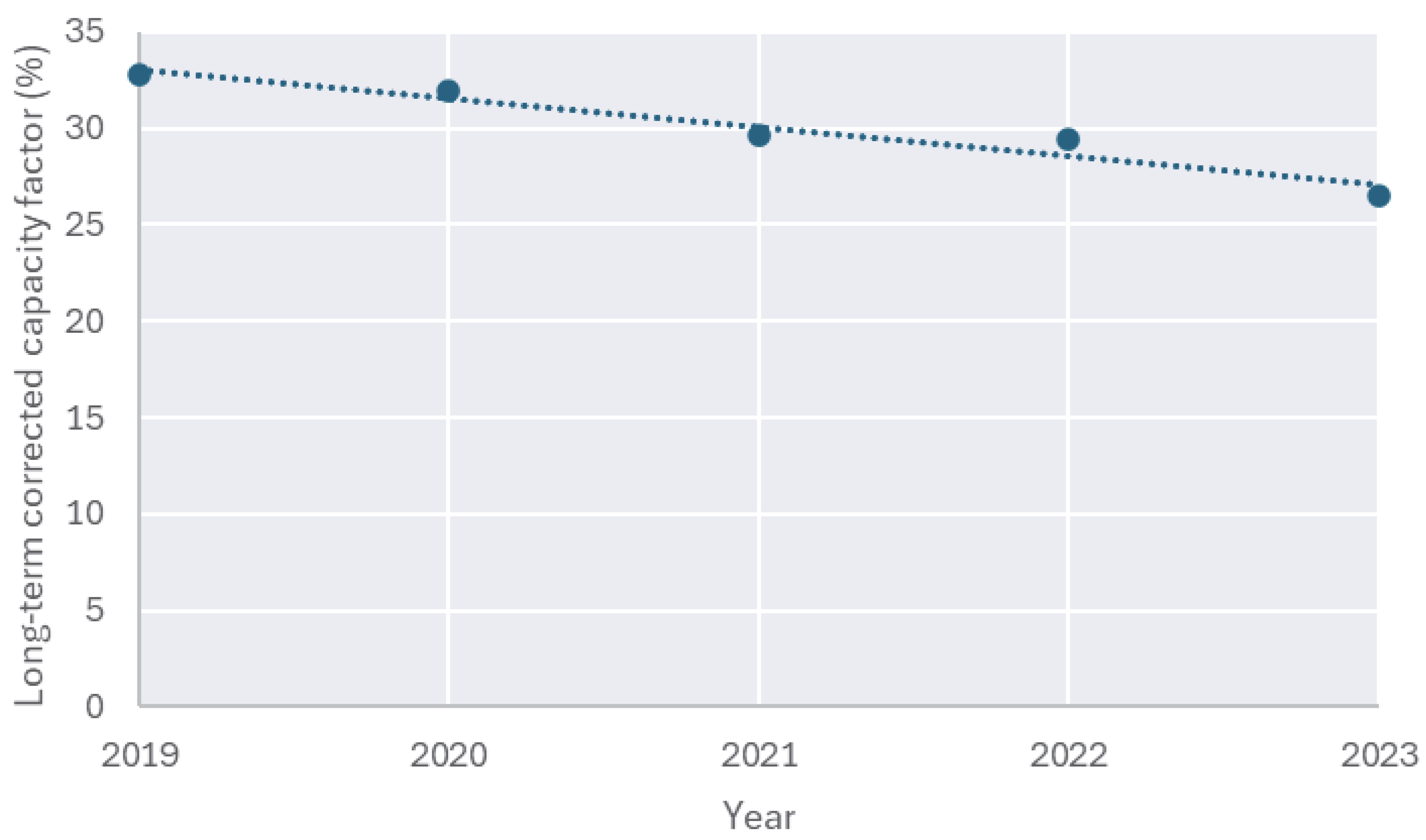The measured capacity factor ${CF}_y$ from the wind farm during the same time period (as recorded in monthly production reports) was then divided by a custom wind index for each year, ${WI}_y$, computed as follows [26]:

$${WI}_y= {\displaystyle \frac{G_y}{\overline{G}}}$$

(1)

$${{CF}_y}^{LTC}={\displaystyle \frac{{CF}_y}{{WI}_y}}$$

(2)

No adjustments were made based on turbine availability or curtailment, since we were assessing overall farm performance for all causes. Past financial records were provided by the client. Expenses were divided into maintenance costs, which arose from service contracts as well as some direct materials and specialists, and other expenses such as administration costs and imbalance charges from the grid operator. The past rates from the Purchase Price Agreements were analyzed to estimate the annual increase. The year-on-year changes for the primary drivers of farm profitability were computed.

2.2. Repowering Options

A review was then conducted of turbines currently on the market that may be used for turbine replacement at this site. Vestas V117-4200 (Aarhus, Denmark), Nordex N133/4.8-4800 (Hamburg, Germany), and Siemens SG 6.6-155-6600 (Munich, Germany) were selected for analysis because they had available performance data and were most likely to be appropriate for the very high wind speeds at the site. Realistic site plans were created, applying provincial regulations for set-back limitations from roads and dwellings as well as special considerations for environmentally sensitive areas. To estimate the power production from new wind turbines, a generalized wind climate (GWC) file was generated using windPRO, using the Matrix MCP method with ERA5 wind speed at 100 m between 31 December 1978 and 15 January 2026 as a reference. The PARK tool was used to estimate the annual energy production (AEP) for the site plans using each type of turbine. A 10% simple reduction was applied.

Capital and maintenance costs were estimated for a full repowering, taking into consideration previous projects for the same client and reported costs of wind farm projects in the news. A Partial Repowering package was also available for the current turbines at the site, for which indicative costs and technical details were provided by the vendor.

2.3. Recommendations

Three options were considered for this farm: continuing with Business as Usual (BaU), Full Repowering with all turbines replaced, and a Partial Repowering package that was offered by a third party for the client’s existing turbines. A financial modeling tool was implemented using the OpenMDAO module (version 3.39.0) in Python (version 3.13.2) to support constrained optimization [27]. The tool takes as inputs the annual energy production for the base year (AEP), the power purchase agreement price (PPA), the annual operating expenses (OPEX), the annual non-O&M expenses (insurance, landowner payments, etc.), the capital costs (CAPEX) for full or partial repowering, and a discount rate. The discount rate is used to account for the time value of money when comparing cash flows at different times. For the repowering scenarios, lost production is applied to the cash flows (3 months for a partial repower, 1 year for a full repower). For Full Repowering only, the decommissioning costs for the previous turbines are applied in the same year. Then, the farm operates as normal. The Partial Repowering scenario has a higher AEP than the BaU scenario (since that was the primary target of the particular Partial Repowering package applied), the Full Repowering Scenario has both higher AEP and lower O&M expenses than the BaU scenario, and all other parameters are the same between each simulation. In the Full Repowering scenario, the farm is assumed to operate for the duration of the simulation, after which the decommissioning costs are applied in the last year and no residual value is assumed. Some of the BaU runs and the Partial Repowering run decommission the farm early. If so, the decommission costs are applied to the intended decommissioning year, and no further costs or profits are assumed for the rest of the simulation.

The non-O&M expenses are assumed to be fixed. The O&M costs for all of the scenarios are assumed to increase by 3% per year. Using a discount rate of 4% for all scenarios, the tool computed the net present value of the expenses (NPV Expenses), and the net present value of the annual energy production (NPV AEP) over the period. The levelized cost of energy (LCOE) was then given as follows:

$$LCOE= {\displaystyle \frac{CAPEX+NPV Expenses}{NPV AEP}}$$

(3)

Financial parameters that apply to all scenarios are reported in

Table 1. Financial parameters that apply to all scenarios.

Parameter	Value
Simulation period (years)	25
Interest rate (%)	4 1
O&M annual increase (%)	3 2
PPA annual increase (%)	1 3
Decommissioning cost	$1500/turbine 4

¹ Expert judgment informed by the client’s specific circumstances re: access to capital. ² Expert judgment. Much lower than the mean from the last 5 years of historical analysis because of extreme outliers due to the COVID-19 pandemic. ³ Statistical historical analysis. ⁴ Expert judgment informed by decommissioning assessments for multiple projects in North America.

. The settings that are specific to each repowering scenario are reported in

Table 2. Financial parameters that apply to the two repowering scenarios.

Parameter	Full Repowering Value	Partial Repowering Value
Capital cost ($/kW)	2000 1	757 3
AEP increase (%)	Modeled (see Section 2.2)	7.6 3
O&M decrease (%)	20 2	0

¹ Expert judgment informed by past projects from the client and news reports of wind projects in the same area. ² Expert judgment informed by more recent projects in the client’s portfolio with turbines of similar sizes. Note that the number of turbines and their age is decreasing, but the installed capacity is increasing, so there are competing factors. ³ Supplied by a vendor.

. For the Business as Usual (BaU) scenario, the rate of AEP decline varied between 0 and 5%. The financial outputs were then computed for each scenario.

Once the financial results were obtained, a reasonable decommissioning year was set for the Business as Usual (BaU) case, and the most promising of the two repowering approaches was selected—this case will be referred to simply as Repowering moving forward. The decisions were based on maximizing the NPV metric rather than minimizing the LCOE, since NPV would allow the client to maximize overall profit at their site. The LCOE was provided as supplemental information to facilitate comparison between this site and other farms in the client’s portfolio which differed in scale.

The relationship between the escalation of the PPA price and the operations and maintenance (O&M) costs represents a structural uncertainty for the model. Firstly, the COVID-19 pandemic caused outliers in operating cost increases that were extremely unusual. As a result, the wind industry in this area is generally struggling at the current PPA price, and the PPA is expected to increase soon. In practice, these two rates are not independent of each other. A range of net present values are therefore reported to show the relationship between profitability and the different rates. The escalation rates for PPA price and O&M costs were excluded from the optimization-based approach used in the next steps because estimating and representing the true uncertainty and the relationship between these two parameters is outside of the scope of this simplified analysis.

2.4. Uncertainty

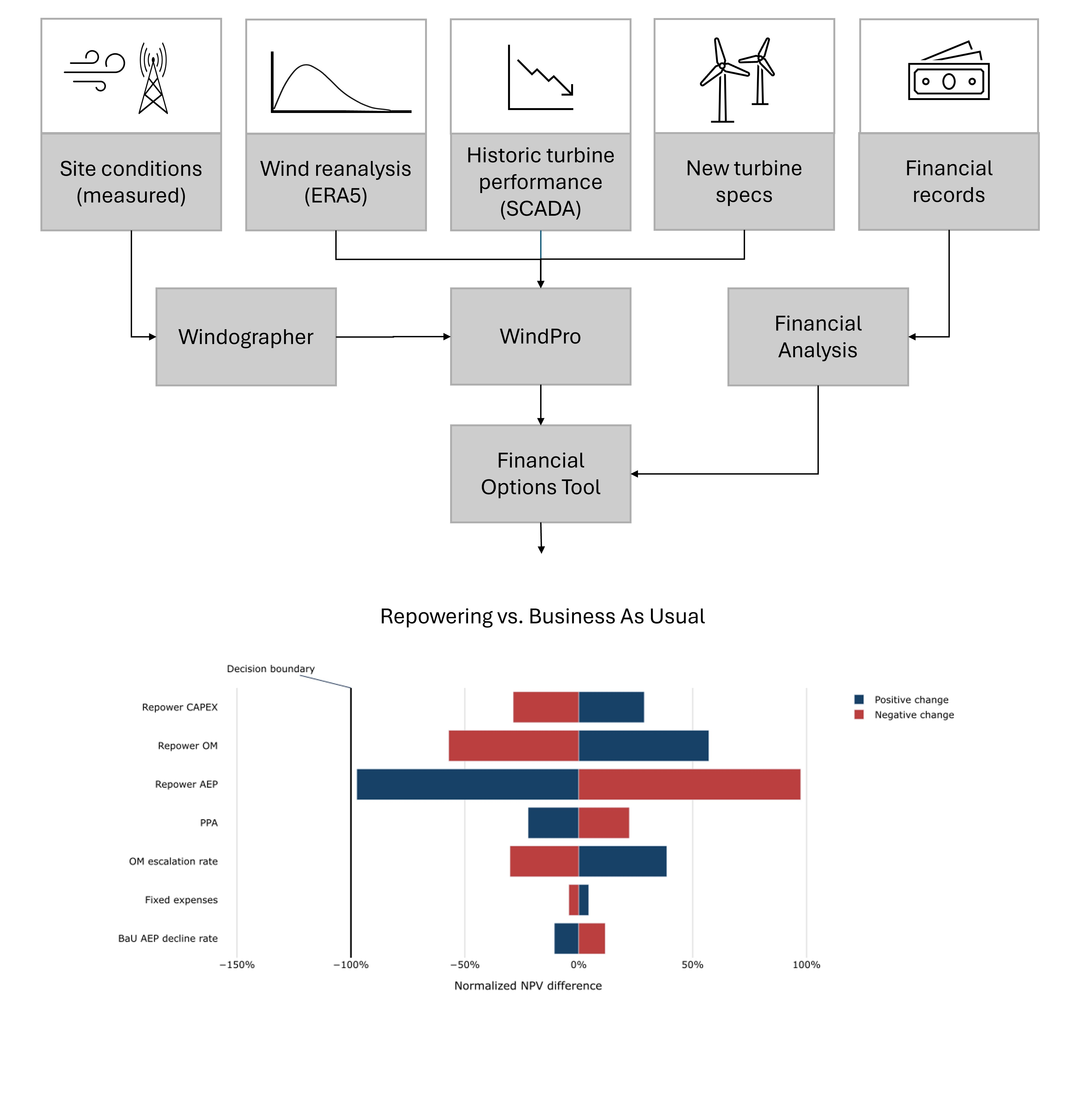
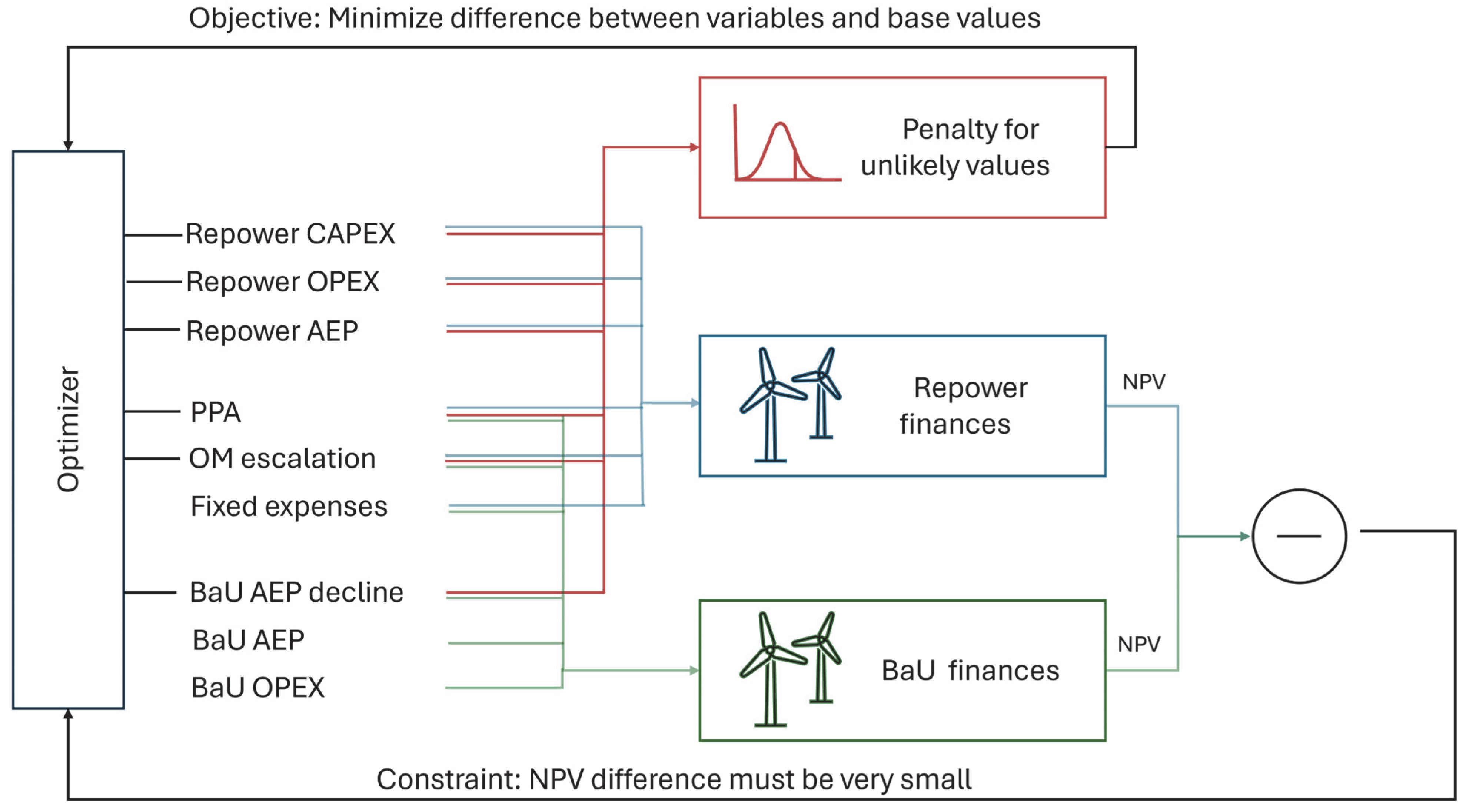
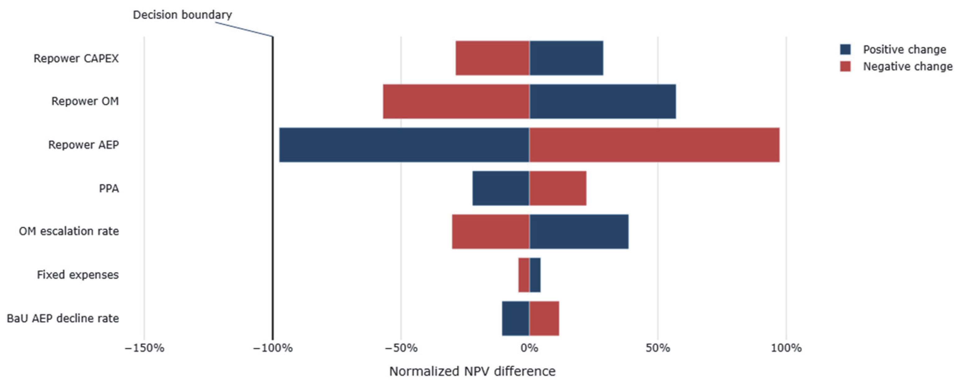
Once the most promising approaches had been identified, the implications of uncertainty were assessed using a sensitivity analysis and decision boundary search. An OpenMDAO optimization problem was constructed with a financial model for both the BaU case and the Repowering case, as well as a component to compute the difference between their net present values (see Figure 1). The uncertainty in the annual energy production of the model was first estimated (

Table 3. Estimated uncertainty for the repowered wind models. The total uncertainty assumes that each source is completely uncorrelated.

Parameter	Estimated Uncertainty (%)
Measurement accuracy	5
Vertical extrapolation	2
Horizontal extrapolation	10
Historic wind climate	3
Turbine performance	5
Plant performance	5
Total	14

), using expert judgment informed by the work of Lee and Fields [28] and a range of general guidance. The uncertainty in each techno-economic parameter was then estimated (see

Table 4. Estimates of one standard deviation for inputs used in the sensitivity analysis and decision boundary search.

Parameter	Estimate of One Standard Deviation
PPA (cents/kWh)	0.2 1
Repowering CAPEX ($/kW)	225 2
Repowering OPEX ($/kW)	20 3
Repower capacity factor (%)	14
BaU AEP annual decline (%)	4.3 4
O&M escalation rate (%)	10 5
Fixed expenses ($)	$55,000 6

¹ Statistical standard deviation from past records. ² Expert judgment informed by NREL’s annual technology baseline [29], past projects from the client, and news reports of wind projects in the same area. ³ Expert judgment informed by NREL’s annual technology baseline [29] and OPEX variation within the client’s portfolio. ⁴ Expert judgment informed by statistical standard deviation from production records, past performance modeling, and feedback from clients on downtime causes and recent O&M investments. ⁵ Statistical standard deviation from past records. ⁶ Statistical standard deviation from past records.

), and the resulting difference in the NPV was reported as a sensitivity chart. Based on the sensitivity results and further discussions with the client, four inputs were identified as both sensitive and substantially uncertain: the PPA (which applies to both cases) along with the CAPEX, OPEX, and AEP of the repowered wind farm. A constraint was added to the optimization problem so that the difference between the NPV of the BaU and the Repowering case was required to be very small. Each of the four inputs were set as design variables, so that when the problem was optimized it would vary those inputs and return combinations that meet the constraint; therefore, for these combinations, since the NPV is almost equal it makes very little difference which option is selected, and if they change a little bit in one direction, Repowering would be the best choice on one side and BaU in the other, i.e., these variables exist on a ‘decision boundary’ between two different recommendations. There are many combinations of values for these inputs that fit that criteria, and the choice of which ones to present to a client is fundamentally subjective. To select which combinations to return, an objective function was defined, the penalty function, which took the design variables as input and returned a higher value when inputs were moved further away from their base (i.e., most likely) values. A flow chart of the resulting optimization problem is depicted in Figure 1.

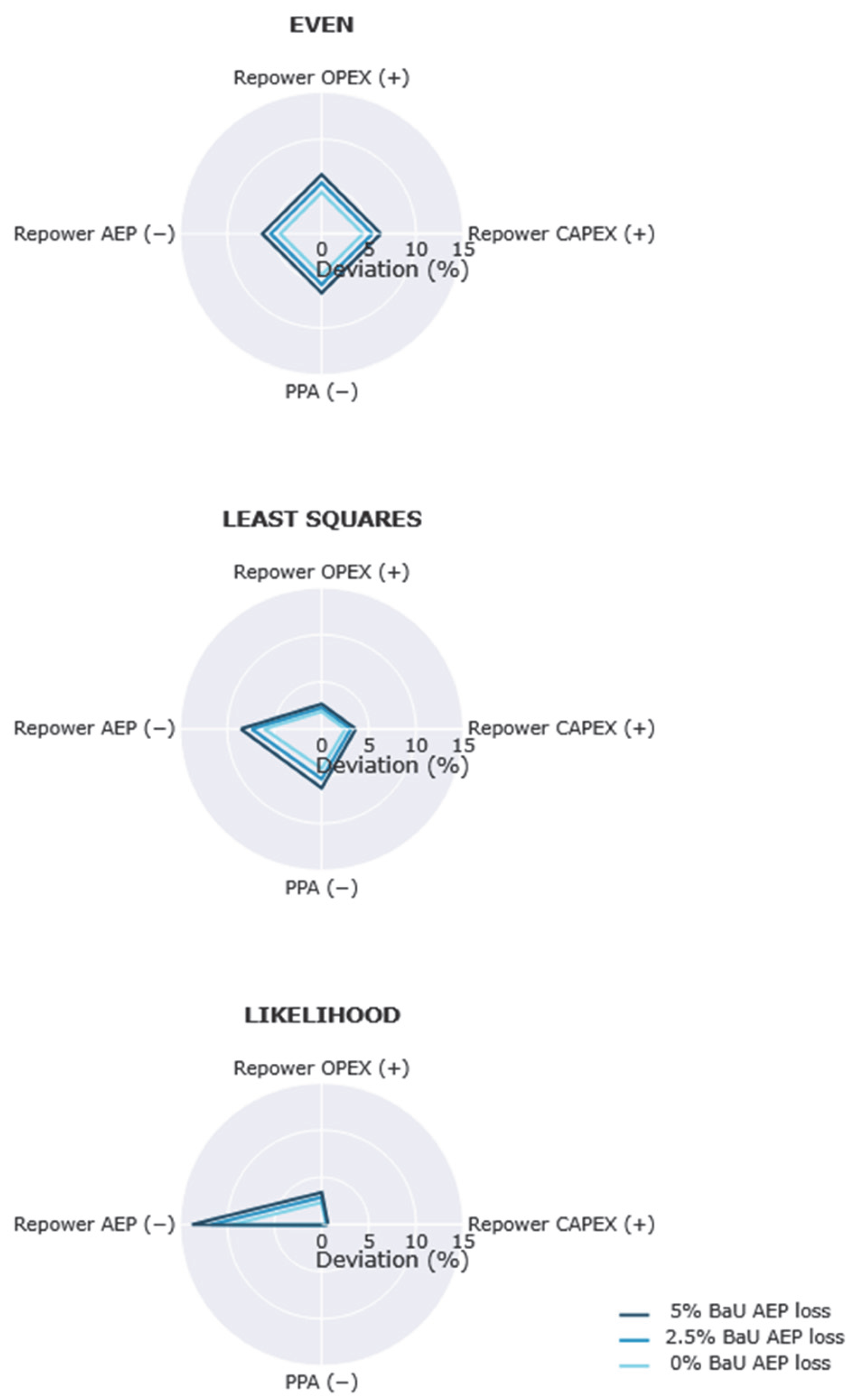
Three different penalty functions were trialed. The first, an ‘Even’ penalty, adjusts all parameters by the same relative amount. The inputs were moved in the direction that would tend to reduce the difference between the two scenarios (for example, the AEP of the repowered farm was reduced and the repowering CAPEX was increased, because both reduce the profitability of Repowering compared to BaU). The penalty was set to the magnitude of that relative difference. The second, the ‘Least Squares’ penalty, takes advantage of differing model sensitivity for each input to try to reduce the total deviation across all variables by disproportionately modifying the variables to which the model is most sensitive (because the more sensitive the model is to a particular variable, the less it needs to be changed in order to create a given change in NPV). The differences are summed as squares to nevertheless disincentivize extreme deviations for any one variable. This penalty function, $p\left(x_i..x_N\right)$, is therefore computed as the sum of the squares of the relative difference between the current value of each of the design variable ($x_i$) and their base values ($x_{0i}$) as follows:

$$p\left(x_i\dots x_N\right)=\sum _{i=1}^N{\left[{\displaystyle \frac{x_i-{x_0}_i}{{x_0}_i}}\right]}^2$$

(4)

The first two penalties implicitly assume that each input variable has the same relative uncertainty. In the last, the ‘Likelihood’ penalty, this uncertainty is explicitly modeled and allowed to differ. It assumes a normal probability distribution, takes as an additional input an estimate of the standard deviation of each input ${\sigma }_i$, and then computes the probability of each combination of inputs. The result is multiplied by negative one so that the likelihood is maximized by the optimization problem:

$$p\left(x_i\dots x_N\right)=-\prod _{i=1}^N{\displaystyle \frac{1}{\sqrt{2\pi }{\sigma }_i}}\mathrm{e}\mathrm{x}\mathrm{p}(-{\displaystyle \frac{{(x_i-{x_0}_i)}^2}{2{{\sigma }_i}^2}})$$

(5)

Because products are not numerically stable, tending to converge quickly to zero or infinity, there is an increased risk of floating-point errors when using a product. Therefore, this penalty function is implemented using the log-likelihood; the logarithm transforms the product into a sum, and maximizing the log-likelihood is equivalent to maximizing the likelihood because the natural logarithm is a strictly increasing function.

The COBYLA algorithm was used to solve each optimization problem, and the results are shown on polar plots. The problem was solved separately for different levels of annual AEP loss in the existing farm because that is something that can be evaluated regularly as the farm continues to operate.

3. Results

3.1. Past Performance

The results of the wind farm performance analysis are shown in

Table 5. Error metrics for validation of performance model. The range for all turbines for which SCADA data was provided (selected to be the most likely extreme values) is shown here.

Parameter	Wind Speed	Power
Mean bias error	−5–+2%	−3–+4%
Root mean square error	17–19%	37–43%
Cross-correlation coefficient	0.93–0.94	0.91–0.93

and Figure 2. The site is a complex coastal site, in which all turbines and the met mast are within 1 km of the shoreline, some much closer than others, and some exposed from multiple directions. The simple assumptions of this windPRO model were not able to capture these complex dynamics completely, which is expected [30], leading to remaining bias for some turbines and high root mean square error of 43% for turbine power comparisons at 10 min resolution. However, the results are being used for annual comparisons. A 43% RMSE error at 10 min scale translates to 0.2% uncertainty in annual sums if all measurements are uncorrelated, or 2.3% uncertainty if we consider the measurements to be correlated within each 24 h period. Averaging across all of the turbines at the farm will also reduce the impact of the bias errors, but without a full set of SCADA data it is not known by how much. Practically speaking, the sampled locations were chosen to represent the most likely outliers, given the complex coastline and wake effects, so the bias at the farm level is expected to be less than 4%.

Table 6. Average year-on-year differences in wind farm PPA rates, production, and service fees.

Parameter	Average Year on Year Change (%)	Standard Deviation (%)
PPA	0.9	2.9
Normalized production	−5	4.3
Service fees	5.8	10

shows the average year-on-year change for three key drivers of farm profitability: the rate paid to the operator for produced electricity, the farm energy production, and the fees paid by the operators to maintain their service contract. The economic analysis showed that while turbine performance decline is likely contributing to a reduction in profit, it is not the only factor. The cost of maintenance also increased faster than the increase in the rates paid for electricity over the same period. This can be partially attributed to a period of high inflation related to the COVID-19 pandemic and other global events. The Purchase Price Agreements (PPAs) were signed well in advance of those events and did not anticipate such high inflation rates. There is an observable decline in production but also year-on-year variation. Substantial investments were recently made to reduce turbine downtime, and we do not yet know how successful those investments will be. We therefore considered 0%, 2.5%, and 5% decline throughout the next steps.

3.2. Repowering Options

The layouts for three different types of turbines, all designed for high wind speeds, yielded capacity factors between 44 and 50% and annual energy productions (AEPs) between 48,600 and 57,800 kWh (see

Table 7. Specifications and energy production of realistic wind farm layouts using three different types of turbines.

Turbine	Hub Height (m)	Number of Turbines	Capacity Factor (%)	AEP (kWh)
Siemens SG 6.6-155-6600	122.5	2	50	57,800
Nordex N133/4.8-4800	78.0	3	45	57,100
Vestas V117-4200	91.5	3	44	48,600

). The differences in capacity factors between the different turbine layouts are partially due to how well matched the estimated power curves are to the wind at the site, partially due to hub heights and terrain effects and partially due to wake effects. The modeled capacity factors are very high for an onshore wind site. This is due to exceptionally strong winds in the area; a neighboring wind farm using turbines with similar rated power and hub heights reports a capacity factor of approximately 50%. The Vestas turbines were used as the basis for the next steps to provide a conservative estimate.

3.3. Recommendations

If the estimated 2.5% annual decline in production for the wind farm and all other assumptions hold true, the wind farm would be expected to remain profitable for 8 more years (see

Table 8. Financial profitability of Business as Usual case for different annual declines in production, assuming optimal decommission planning.

Output	0%	2.5%	5%
Years of continued production	>10	8	5
Net Present Value	3,900,000	2,000,000	1,300,000

). Without any decline, of course, the wind farm can operate for a long time into the future, but this is practically unlikely. Conventional wisdom suggests that wind turbines will exhibit a ‘bathtub’ curve where performance decline increases towards end of life. If the recently observed 5% continued, there would be 5 years of profitability. Based on these results, year 9 was selected as the decommissioning year for the next steps in the analysis for the BaU scenario, with the understanding that if the client chose to continue operating, they would track performance decline and decide on the basis of that information along with other practicalities.

The Partial Repowering option for this client’s turbines, which was primarily focused on increasing annual energy production rather than extending useful life, was found to be far less profitable than Full Repowering and worse than operating with Business as Usual (see

Table 9. Financial performance for the wind farm in two repowering cases.

Output	Partial Repowering	Full Repowering
Payback period (years)	N/A	11
NPV ($)	−4,700,000	10,000,000

). This is partly because the annual profit from the current turbines is now limited due to the historic imbalance between PPA price and O&M expense escalation. By contrast, the Full Repowering case was more profitable than Business as Usual. This can be attributed to the large increase in capacity factor and overall energy production that is expected from bigger turbines and higher hub heights at this site.

A range of net present values for the BaU and repowered scenario (see

Table 10. Net present value of the Business as Usual (BaU) scenario with a range of PPA price escalation rates (top header) and O&M escalation rates (side header).

O&M/PPA Escalation (%)	0	1	2	3
0	2,530,000	3,200,000	3,910,000	4,650,000
1	2,140,000	2,810,000	3,520,000	4,260,000
2	1,730,000	2,400,000	3,110,000	3,850,000
3	1,300,000	1,970,000	2,680,000	3,420,000
4	850,000	1,520,000	2,230,000	2,970,000
5	370,000	1,040,000	1,750,000	2,490,000
6	−130,000	540,000	1,250,000	1,990,000

and

Table 11. Net present value of the repowering scenario with a range of PPA price escalation rates (top header) and O&M escalation rates (side header).

O&M/PPA Escalation (%)	0	1	2	3
0	8,490,000	15,210,000	22,990,000	32,030,000
1	7,050,000	13,770,000	21,550,000	30,590,000
2	5,390,000	12,110,000	19,890,000	28,930,000
3	3,470,000	10,190,000	17,970,000	27,020,000
4	1,250,000	7,970,000	15,750,000	24,800,000
5	−1,320,000	5,400,000	13,180,000	22,230,000
6	−4,300,000	2,420,000	10,200,000	19,240,000

, respectively) show that most cases are profitable within a range of 0–3% for the PPA escalation rate and 0–5% for the O&M escalation rate, if the other parameters remain at their base values. Statistically speaking, the PPA may decline and the O&M escalation rate may exceed 5%. However, this would most likely jeopardize the profitability of wind energy across the province, not just for this site, and for such financial conditions to be sustained over 25 years this is not considered to be very likely in practice.

3.4. Uncertainty

The financial model was most sensitive to the repowered AEP (Figure 3), suggesting that if the AEP is substantially over-estimated then continued operation may be preferred. When all parameters changed evenly, a 4–7% difference was sufficient depending on the assumed loss in the base AEP. When multiple parameters were varied (Figure 4), combinations where variables shifted 1–14% were sufficient to change the best outcome. When the Least Squares penalty function was employed, the optimizer favored the repowered AEP and PPA. Because the PPA is considered less likely to vary than the OPEX of the repowered wind farm, the likelihood penalty function selected a combination with a smaller change in PPA and larger change in repowered OPEX as the most likely future situation where it would be better not to repower. One aspect that could be misinterpreted when viewing the polar plot is the tendency of the optimizer to disproportionally vary the inputs to which the model is most sensitive when using the Least Squares and Likelihood penalty functions. This results in the smallest combined deviation from the base values, but when viewed as a polar chart it may give the false impression that there is more ‘room to move’ without changing the outcome for the variables which are further from the center of the polar chart. That is not the case at all: variables tend to show up further from the center of the polar chart when they have a greater impact on the NPV, which actually implies less room to move without changing the outcome, and when the penalty function is less sensitive to them.

4. Discussion

Based on the results from this case study, full repowering was recommended to the client. Their next steps would typically include updating their environmental assessments, engaging an engineering team and manufacturers to put together a more detailed site plan with real quoted costs, speaking to power purchasers to seek a new or extended Purchase Price Agreement, reaching out to the utility to ensure that the transmission lines are able to take on additional power, and speaking to any impacted neighbors. The results of the uncertainty analysis for this site suggest that changes in the energy production at the repowered site, for example, if a different turbine is ultimately used, have the greatest potential to change the best approach for this site. This may motivate earlier or greater investments into a firm decision for the type of turbine to be used and a detailed assessment into its expected energy production. For example, although there is historic data at the site, it is far away from some of the turbines and not at hub height, so further wind resource measurements may also be conducted to match the proposed hub heights of the new wind turbines; this would allow a wind resource assessment that combines both data sets to give the best forecast. As new estimates of the key inputs such as repowering CAPEX and AEP are received, their impact can be partially assessed. If all values stay within the boundaries of any of the decision boundary charts, then the clients have some assurance that they are still proceeding along the best path. If all values are equal to or exceed the boundaries, then the client should change paths. If it is a mix, then re-computing a new decision boundary chart with new base values and sensitivities would be recommended.

An anonymous case study is presented in this work because it demonstrates the applicability and utility of this decision-making framework in a fully realistic context. However, because anonymity was required in order to use the real data, which included avoiding site-specific information that might indirectly identify the site, this limited methodological transparency. Notably, it was not possible to identify all the data sources that were used nor explain how methodological practice guidelines were applied to this site’s specific context. It also was not possible to publish the underlying data sets. We acknowledge this as a limitation of the case study presented. We call for future work to demonstrate this process on fully open data to complete what was shown here. That said, many of the approaches used in this study have been reported in the literature previously, particularly the use of windPRO [31]. windPRO is an industry standard software for wind farm planning [32]. It offers multiple modeling approaches that are tuned to the specific features of the site; more complex methods are more likely to be necessary for regions with complex terrain, forests, or oceans [30,32]. The relatively simple modeling choices used in this study are broadly appropriate for pre-screening exercises but would need to be validated for each location. This approach is not suggested for bankable pre-construction estimates, with those left as future work during later planning stages. The use of a computational fluid dynamic model may be needed for this site in the future due to its complex coastal location.

This decision-support approach differs from other workflows in that it uses relatively advanced techniques to analyze turbine performance and potential energy production at the site, which allows it to account for site-specific details such as terrain roughness and updated regulations for setback conditions, but the results of those analyses are then simplified into a few key metrics which feed into a relatively simple financial model. In the authors’ experience, a simple financial model is often appropriate for these early-stage decisions because the focus is on the big picture at that stage. The simplicity of the model also makes it more efficient and reliable to apply optimization-based techniques. In this method we use optimization to seek ‘decision boundaries’ because this supports a more thorough understanding of the ‘breathing room’ that exists before the chosen approach needs to be re-evaluated. The optimization problem is solved in under a minute when running on a standard PC, which is broadly comparable to a simple Monte Carlo or Real Options analysis. However, in later planning stages when the level of financial detail would likely increase, the decision-boundary search may not scale very well; processing times tends to increase rapidly as the number of variables increases in an optimization problem (the so-called curse of dimensionality), and a more detailed problem formulation may have discrete points or more complicated gradients which can impair the rapid convergence of the optimizer. In addition, the simplifications limit the accuracy and realism of the financial model. For example, it does not incorporate fully market-driven price fluctuations. So, overall, this approach is more applicable to the earlier stages of decision-making on this topic.

In the future, the framework could be further developed so that this model transitions seamlessly to more advanced methods during future planning stages. Real options analysis may be a particularly good fit in future planning because it can continue to support the possibility of multiple choices and timelines. Bayesian approaches may also be a good fit due to their ability to formally assimilate a range of data sources with different uncertainties and formally update when new data arrives. There are many parameter combinations that exist at the decision boundaries, and the penalty functions used to select the ones shown here are the result of a subjective judgment as to which combinations may be most helpful to show to the client. Other boundaries may also be valuable, such as the boundary where the project breaks even at the chosen discount rate. The choice of a polar plot is also subjective. The use of other penalty functions and plots is also suggested as future work.