Abstract
This article presents a methodology for the synthesis of horizontal-axis wind turbines operating on the principle of lift. The profile geometry is synthesized using the Vortex–source distribution method following Glauert’s approach. The blade shape is developed using the Blade Element Momentum Theory. Efficiency is determined with Computational Fluid Dynamics. The methodology uses a multifactor numerical experiment, with the objective function defined as maximizing lift-to-drag ratio of the blade profile. Validation of the obtained power curves is performed with QBlade and XFoil and confirmed experimentally on a laboratory test bench. The proposed methodology demonstrates improved accuracy in predicting the power coefficient and the optimal operation regime of horizontal-axis wind turbines at low Reynolds numbers.
1. Introduction
In recent years, interest in renewable energy sources and electricity generation from them has increased significantly. The reason is that the combustion of fossil fuels releases harmful emissions, which lead to heat retention in the atmosphere and global climate change. Wind energy is one of the most widespread renewable energy sources. Wind turbines with either a horizontal (HAWT) or vertical (VAWT) axis of rotation are used to harness wind energy, converting it into mechanical or electrical power. Wind turbines operate based on two main principles: lift and drag. In drag-based turbines, the pushing force of the wind drives the rotor. In lift-based turbines, rotor torque is generated by the pressure difference across the blade surface. Such turbines achieve higher rotation speeds and lower torque at optimal operating conditions. They are less expensive than turbines operating on the active principle, which in most cases use disc generators suitable for low rotation frequencies and high torque.
The growing interest in wind turbines has led to an increase in research activity in this field, laying the groundwork for the development of more efficient wind turbines—an objective shared by manufacturers. Previous studies have shown that the efficiency of turbines operating on the lift principle depends primarily on the aerodynamic quality of the blade cascade. This motivated researchers to focus on improving the aerodynamic performance of the airfoil, employing various numerical methods.
According to the blade cascade theory, the optimization of a wind turbine is performed through a sequence of synthesis and analysis tasks. In the synthesis step, the blade profile is defined by specifying key parameters, including chord length, angle of attack, curvature, and maximum thickness. In the analysis step, the efficiency of the resulting blade geometry is evaluated, including the calculation of lift and drag coefficients, velocity, and pressure distributions along the blade surface. Both tasks use numerical and CFD-based methods.
Numerical methods rely on potential flow theory, such as the Vortex Panel Method [1,2], Singularity Method [3,4], Glauert’s Vortex Distribution Method [5,6], and surrogate-potential-based optimization [7,8]. Numerical methods based on potential flow theory are used to model steady, irrotational flow around solid, impermeable bodies (such as turbine blades). The streamlined surfaces are divided into small panels, each assigned its singularity (vortex or source). By adjusting the intensity of these singularities, the impermeability boundary conditions are satisfied by eliminating the normal component of velocity on the surface. In airfoil synthesis, the suction and pressure sides are treated as continuous streamlines. Depending on the nature of the problem—whether synthesis or analysis—two different approaches are employed. In synthesis, the vortex intensity distribution along the chord is prescribed, and then, using an iterative scheme, the velocity distribution along the pressure and suction sides of the profile is calculated. Based on the relationship between the streamlined shape and the velocity distribution, the airfoil geometry is determined. In the analysis task, the airfoil geometry is given, and the vortex intensity distribution along its contour is computed. Numerical methods based on potential flow theory are suitable for preliminary, coarse estimation of airfoil performance, as they do not account for viscous shear forces, the boundary layer, or the flow separation point on the surface. This makes them appropriate for initial design stages. To model viscous forces and the boundary layer on the airfoil surface, integral methods (such as those by Thwaites [9] and Head-Smith [10]) are employed. These methods enable a preliminary estimation of the likelihood of flow separation.
CFD-based methods account for viscosity, vortices, and turbulence. These methods include CFD-driven optimization [11], adjoint-based optimization [12,13,14], surrogate-based CFD optimization [15], and shape morphing [16]. CFD-based synthesis methods use an existing database obtained from numerical modeling of various airfoil profiles. A target function is defined, such as maximizing lift or the lift-to-drag ratio (L/D). The relationship between the flow parameters around the blade shape is approximated. Optimization is carried out using a design of experiments (DoE) approach, which defines the range and step size for variation in the studied parameters. Unlike DoE, surrogate-based optimization methods use a pre-existing dataset to train the surrogate model. For example, Airfoil Tools [17] provides free access to aerodynamic characteristics of various airfoil types with high L/D ratios under different Reynolds numbers—such as NAS LS(1)-0417, Selig S1223, Eppler E423, RAF32, and others. In turbine blade design, this data can be used to approximate the aerodynamic shape at each radial cross-section in order to achieve maximum lift and L/D ratio values.
The choice of optimization methodology determines both the accuracy and computational time of synthesis and analysis. Methods based on potential flow theory (such as the Vortex Panel Method, Singularity Method, Glauert’s Vortex Distribution Method, Schmitz [18], BEM [19], etc.) are most preferred during the initial stages of design due to their simpler algorithms and ability to provide a fast preliminary evaluation of the geometry under study. These methods are integrated into software tools for wind turbine synthesis, such as XFoil [20], QBlade [21], and ProPan [22]. QBlade and XFoil are widely used for preliminary design of wind turbine rotors, due to their free licenses. The software uses panel methods combined with integral boundary-layer models (IBL) developed by Thwaites [9], Head-Smith [10], and Eppler [23]. These models have limited universality. They are semi-empirical and calibrated for higher Reynolds numbers, relying on empirical correlations. At low Reynolds numbers, the boundary layer may remain laminar over large sections of the body or separate, forming laminar separation bubbles [24,25,26]. Accurate prediction in such cases requires different methods, since IBL often misestimates transition and separation points. In practice, potential flow-based methods are often combined with CFD methods. In such cases, the synthesized rotor geometry is integrated into a numerical CFD model, enabling higher accuracy in computational analysis. This allows for the simulation of the boundary layer around the surface of turbine blades through the generation of a sufficiently fine computational mesh. Unlike potential flow methods, CFD methods solve the Navier–Stokes equations [27], which describe the motion of a viscous Newtonian fluid. These equations enable modeling of the boundary layer around turbine blades, flow turbulence, and tip vortices—all of which significantly influence the efficiency of the turbine.
Table 1 presents the power coefficient (Cp) values obtained after rotor optimization of HAWTs by various authors over the past 13 years. As observed, researchers predominantly use synthesis methods based on potential flow theory. Boundary layer modeling around the airfoil is typically performed using integral methods through the XFoil software. For rotor synthesis, the most commonly used tool is QBlade, which employs the BEM method. The achieved Cp values vary depending on the optimization method, airfoil shape, and software applied. The highest reported value, Cp = 0.560, was achieved by Quarona et al. [28] using the Lifting Line Method [29] and the ProPan software, which is based on potential flow theory. Lower Cp values were reported by Koç et al. [30] (0.500), who used CGA and BGA optimization algorithms combined with the BEM method, and by Pourrajabian et al. [31], who also reported Cp = 0.500 using BEM. S. Poole et al. [32] achieved Cp = 0.510 using BEM along with boundary layer modeling in XFoil. All three studies employed the NACA4412 airfoil. Bekkai et al. [33] achieved Cp = 0.450 using the SG6043 airfoil and the QBlade and ANSYS Fluent 2010 [34] programs. Radi et al. [35] reported Cp = 0.470, using a genetic algorithm (GA), the NACA2424 airfoil, and XFoil. Boudis et al. [36] also reached Cp = 0.470 using Fluent Adjoint Solver v.2020 combined with BEM and the S809 airfoil. Other results include: Kriswanto et al. [37] with Cp = 0.405 for NACA4412 and NACA2412 airfoils using the Taguchi DOE method [38]; Mohammadi et al. [39] with Cp = 0.410 using BEM and aerodynamic data from 43 different airfoils; Al Abadi et al. [40] with Cp = 0.440 using NREL and S809 airfoils through Schmitz and BEM methods; Xin Shen et al. [41] with Cp = 0.440, using the S890 airfoil, the Lifting Surface Method [42], and a genetic algorithm.

Table 1.
Comparison of the aerodynamic optimization of HAWTs from various studies.
In general, most Cp values reported were obtained using simplified models for airfoil synthesis that do not accurately account for the influence of the boundary layer. Furthermore, no validation through physical experiments on laboratory test rigs or in field conditions has been performed. Studies of HAWTs in wind tunnels [44,45] have shown that at low Reynolds numbers (Re < 1 × 10⁶), Cp values typically range from 0.08 to 0.38 (see Figure 1). This casts doubt on the reliability of many results presented by the authors in Table 1. For instance, at Re = 4 × 10⁴, Bekkai et al. [33] report Cp = 0.450, while the expected value should be around 0.298. Radi et al. [35] and Boudis et al. [36] report Cp = 0.470 at Reynolds numbers between 3 × 10⁵ and 1 × 10⁶, whereas realistic values should be closer to 0.257 and 0.365. According to Umar et al. [43], Cp = 0.450 at Re = 3 × 10⁵, although the value should be around 0.257. Even greater discrepancies are seen in Pourrajabian et al. [31] and Koç et al. [30], who report Cp = 0.500 at Re ≈ 1.6 × 10⁶, which is significantly above the expected upper limit of 0.38. Poole and Phillips [32] report Cp = 0.510 at Re = 8 × 10⁵, while the realistic value should be around 0.35. Similarly, Al-Abadi et al. [40] report Cp = 0.440 at Re = 6.65 × 10⁵, which is approximately 0.1 above the expected range. As illustrated in Figure 1, the red curve shows the trend of the power coefficient as a function of Reynolds number, based on experimental data [45]. The blue curve shows the Cp values obtained after optimization. The labels of the data points refer to the author number in Table 1. The Cp values obtained after the optimizations are significantly higher, especially at Raynolds < 2.6 × 10⁶. According to the graph, there is a coincidence only at Reynolds > 3.4 × 10⁶, the so-called self-similarity zone. This indicates that the numerical methods used are unable to capture the dependence of aerodynamic performance on wind speed.
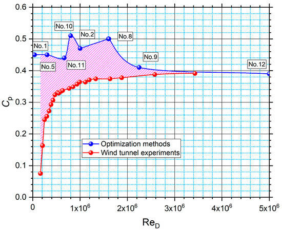
Figure 1.
Comparison of the power coefficient obtained at different Reynolds numbers [45].
This publication presents a methodology for the synthesis and optimization of HAWTs rotors that is more accurate than panel methods and faster than full CFD approaches. The methodology begins with the synthesis of the aerodynamic profile using the Vortex–source distribution method, followed by 2D analysis with CFD. This approach enables the creation of a database, which is used for optimization of the blade shape. The turbine rotor is finally designed using the BEM method in combination with the obtained polar curves of the blade profile. The aim of this methodology is to overcome the limitations of the IBL methods and improve the accuracy of the BEM method in predicting the power coefficient of HAWTs at low Reynolds numbers. Compared to Reduced Order Models (ROMs) [46] and adjoint solvers, the proposed methodology requires fewer computational resources, does not require training, and can be directly applied to rotors with varying diameters and blade numbers. Unlike adjoint solvers, it is not constrained by a fixed CAD geometry and flow velocity, allowing faster optimization of the blade shape.
2. Airfoil Shape Optimization
2.1. Optimization Methodology
The methodology is illustrated in the block diagram in Figure 2. The synthesis of the blade profile is carried out using Glauert’s Vortex Distribution Method, by setting the flow velocity Cw and the coefficients, A0, A1, B0, and B1, which define the distribution of the vortex intensity (x) [47] along the length of the camber line. Initially, it is assumed that the camber line coincides with the chord Lr. The relationship between the velocity distribution along the blade contour and its shape is defined by Equation (1) [47]:
where are the velocity components in the y and x directions, dy/dt and dx/dt are the first derivatives, with respect to time, of the coordinates of an arbitrary point along the profile contour. The camber line of the profile is divided into k vortex filaments. To construct the profile shape, the influence of these vortex filaments on the camber line is taken into account. As the vortex filaments are traversed in the range from 1 to k, the geometric center of the current vortex filament becomes the observation point, while the geometric centers of the remaining vortex filaments serve as influence points. In short, at each point along the camber line, the inductions from the surrounding vortex filaments are calculated. During the first iteration, the camber line coincides with the chord, and the velocity component matches the flow velocity Cw. The relationship between the velocity component and the coordinate x is given by Equation (2) [47]:
where x−x′ is the distance between the current observation point and an arbitrary influence point, is the length of the observed vortex filament, is the vortex intensity at the current influence point, and r is the absolute length of the radius vector from the current observation point to an arbitrary influence point. The coordinates of the camber line, together with the geometric centers of the vortex filaments, are displaced in the y direction using Equation (3) [47]:
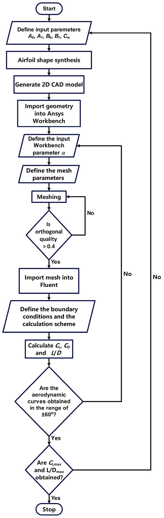
Figure 2.
Block diagram illustrating the airfoil optimization process.
In the next iteration, when calculating the velocity components, the curvature of the camber line (the coordinates yi) is also taken into account, using Equations (4) and (5) [47]:
where y−y′ is the distance between the current observation point and an arbitrary influence point in the y direction. The updated coordinates of the camber line along the y-axis are calculated using Equation (6) [47]:
The procedure is repeated until the difference between two successive approximations becomes sufficiently small. For the vortex filament intensity, Glauert’s geometric series is used [47]:
where (x) = acos ().
The airfoil profile is constructed by enveloping the infinitely thin airfoil formed by the vortex layer with a body of aerodynamic shape. For this purpose, a source layer with appropriate intensity is applied along the camber line, which now serves as the line of influence [47]:
Now, at the observation points, both velocities induced by the vortex layer and the velocity components and must be taken into account [47]:
The equation of the contour of the full airfoil profile is as follows [47]:
where the plus sign (+) refers to the suction side, and the minus sign (−) refers to the pressure side of the airfoil.
The blade profile is synthesized using the computer program MATLAB 2022a according to the methodology described above. The nondimensional coordinates of the finalized full profile are multiplied by the chosen chord length Lr, after which they are imported into the CAD system SolidWorks 2022. The contour of the full profile is drawn using a cubic spline. The completed geometry is then prepared for CFD analysis by importing it into the Design Geometry module in Ansys Workbench 2022. The angle of attack of the profile, the dimensions of the surrounding computational domain, and its boundary conditions are set.
The next step is importing the geometry into Ansys Meshing 2022, where the main parameters of the computational mesh are defined. If the orthogonal quality of the generated mesh is lower than expected, the primary mesh parameters are adjusted.
The completed computational mesh is imported into the Ansys Fluent 2022 module, where the flow velocity, turbulence model, ambient pressure, and the outlet pressure of the computational domain are specified. Calculations of the lift and drag coefficients, CL and CD, are performed for several values of the angle of attack α and recorded in a text file. The angle of attack at which the maximum L/D ratio occurs is identified.
The described procedure (see block diagram in Figure 2) is repeated by assigning new values of the coefficients A0, A1, B0, and B1, until maximum values of the lift coefficients and the L/D ratio are achieved.
2.2. CFD Setup for Profile Evaluation
Figure 3 and Figure 4 show the schematic diagram with the overall dimensions of the computational domain and the mesh used to calculate the aerodynamic characteristics of the studied airfoil profiles. The domain dimensions, boundary condition types, and geometric parameters of the computational mesh (Table 2 and Table 3) are defined according to recommendations from specialized literature [48], taking into account their impact on aerodynamic performance. Key parameters that determine mesh quality include orthogonal quality, the aspect ratio between long and short cell edges, and the volume ratio between neighboring cells. Recommended values for these parameters are summarized in Table 4. A mesh generated with poorly defined parameters may result in inaccurate outcomes or difficulties in achieving solution convergence.
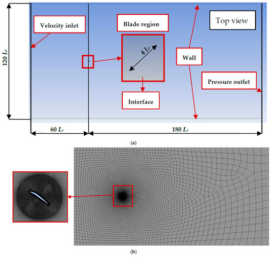
Figure 3.
(a) Overall dimensions of the surrounding 2D computational domain, Lr = 200 mm; (b) Computational mesh used.
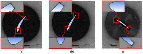
Figure 4.
Computational mesh around airfoils at different stages of the shape optimization process: (a) Initial design; (b) Refined design; (c) Final design.
Table 2.
Boundary layer meshing parameters around the airfoil.
Table 3.
Mesh parameters of the computational domain.
Table 4.
Mesh parameters based on best practices.
For accurate prediction of the boundary layer and flow separation from the streamlined surface of the profile, a sufficiently fine mesh resolution is required in the near-wall region (Figure 4). Schlichting and Gersten define this mesh resolution using the dimensionless coefficient y+ [51]:
where ywall (m) is the normal distance from the streamlined surface to the geometric center of a cell in the first layer, ut (m/s) is the tangential velocity at the cell’s geometric center, and υ (m2/s) is the kinematic viscosity of the working fluid. It has been proven that, for accurate boundary layer prediction, the first cell layer should satisfy the condition y+ < 1 [51]. These values can be estimated using the analytical formulas of Frank M. White [52], which are commonly applied to boundary layer calculations around a flat plate. To do this, data such as the flow velocity, the chord length of the airfoil, and the ywall distance are required. The actual y+ values are monitored during the numerical simulation, and if necessary, the mesh resolution is adjusted accordingly.
In the present study, a mesh resolution of 1 μm was specified in the near-wall region of the blade. The predicted y+ values for the flow velocity range Cw = 4, 6, 8, 10, 15, 20, 25, and 30 m/s are 0.017, 0.022, 0.025, 0.028, 0.032, 0.035, 0.037, and 0.041.
The numerical simulations were carried out using k-ω SST turbulence model [53] at angles of attack α = −60°, −55°, −50°, −45°, −40°, −35°, −30°, −25°, −21°, −19°, −17°, −15°, −13°, −8°, −4°, 0°, 4°, 8°, 11°, 13°, 15°, 17°, 19°, 21°, 25°, 30°, 35°, 40°, 45°, 50°, 55°, 60°. The objective functions of the optimization problem are the maximum L/D ratio and maximum lift coefficient CL, while the input parameters are the angle of attack α and the vortex intensity coefficients A0, A1, B0, B1:
In Equation (14), αopt,i refers to the angle of attack at which the current blade profile achieves the maximum L/D. During the optimization process, each blade profile is analyzed sequentially using the Design Point method in Ansys Workbench. For every design point, the input parameters are the angle of attack and flow velocity Cw. The output parameters are the L/D ratio and the aerodynamic coefficients.
To improve the accuracy of the simulation, second-order numerical schemes (Table 5), were used in the discretization of the pressure, momentum, and turbulence equations within each cell of the computational mesh.
Table 5.
Settings of the computational procedure.
2.3. Results of Airfoil Optimization
The data from the optimization were processed using MATLAB 2022a, and the values of the maximum L/D ratio and the maximum lift coefficient (CL) were determined using the built-in fmincon function (function minimization with constraints). The optimal shape of the airfoil was synthesized using the method described in Section 2.1.
Figure 5 and Table 6 show the non-dimensional coordinates of the optimized airfoil, the corresponding vortex intensity coefficients, as well as the non-dimensional locations of the maximum camber along the mean camber line and the maximum airfoil thickness.
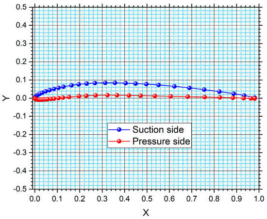
Figure 5.
Optimized blade shape.
Table 6.
Optimized blade parameters.
Figure 6 presents the mesh independence study for different angles of attack. Four different mesh configurations are analyzed: first one has a wall distance y = 1 μm and 4000 nodes; second mesh has y = 2 μm and 4000 nodes; third mesh has y = 10 μm and 400 nodes; fourth mesh has y = 100 μm and 400 nodes. As noted, the changes in L/D gradually converge with mesh refinement. The differences become negligible for wall distances smaller than 2 μm. Numerical calculations of the aerodynamic curves are conducted with the first mesh.
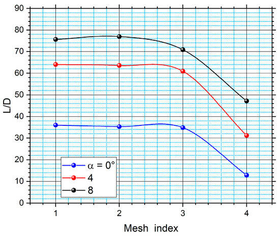
Figure 6.
Mesh independence study.
To validate the proposed methodology, the obtained aerodynamic curves are compared with results from XFoil v.6.61 (Figure 7). The aerodynamic curves showed good agreement at angles of attack greater than 15° and less than −5°. The maximum L/D calculated with XFoil is approximately 128 at an angle of attack of around 6°, while the Ansys Fluent simulations produced an L/D of about 76 at around 8°. The differences in aerodynamic curves are attributed to both the geometric features of the airfoils and the limited capabilities of the IBL methods used in XFoil.
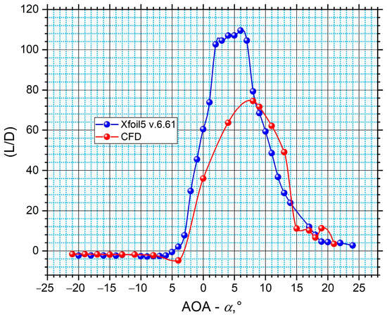
Figure 7.
Comparison of the obtained curves.
3. Blade Design and Rotor Synthesis
3.1. Blade Geometry Generation
The synthesis of the turbine blades was performed using Blade Element Momentum (BEM) theory, which can be viewed as a combination of two separate theories: Blade Element Theory (BET) and momentum theory. BET is used to calculate the aerodynamic forces (lift, drag, tangential, and normal) acting on small individual sections (elements) of the blade. Momentum theory, on the other hand, applies the principle of conservation of momentum to the airflow passing through the rotor disk. For this purpose, axial and tangential induction factors (a‘ and b‘) are introduced, which represent the degree of velocity change Cw as a result of the fluid’s interaction with the rotor. The axial induction factor is used to determine the projection of the relative velocity (W) along the rotor axis (Wa), while the tangential factor determines the projection in the direction of the rotational velocity (Wu), as shown in Figure 8. The vector sum of Wa and Wu represents the relative velocity W, which is used for the calculation of the aerodynamic forces acting on the airfoil at the given blade section: lift (FL), drag (FD), tangential (FT), and normal (FN).
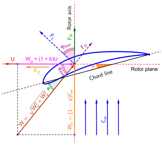
Figure 8.
Flow velocity and force vectors acting on the rotor blade segment under steady-state conditions.
The block diagram of the algorithm used for synthesizing the turbine blades is shown in Figure 9. The input parameters specified are: the maximum rotational speed within the examined range nmax (min−1), the rotational speed increment Δn (min−1), the design rotational speed ncalc (min−1), flow velocity Cw (m/s), air temperature T (K), the main diameter of the rotor D1r (m), hub diameter Dg (m), the number of blade sections Nsec, number of blades Zr, the initial chord lengths at the hub and tip (Lhub and Ltip), tolerance values ξ1 and ξ2, used in the iterative procedure for calculating the induction factors a‘ and b‘ under different operating conditions. The induction factors are initialized with a starting value of zero. The flow angle (rad) is then calculated using Equation (15), which corresponds to the right-angled velocity triangle formed by the components of the relative velocity Wa and Wu (the orange and purple vectors in Figure 8) [54,55,56]:
where the subscript i denotes the current blade section number during the blade traversal. The pitch angle of the airfoil (rad) is calculated as the angle between the relative velocity vector W and the chord Lr at the given section. It is defined as the difference between the flow angle and the optimal angle of attack αopt (rad), at which the airfoil achieves its maximum L/D:
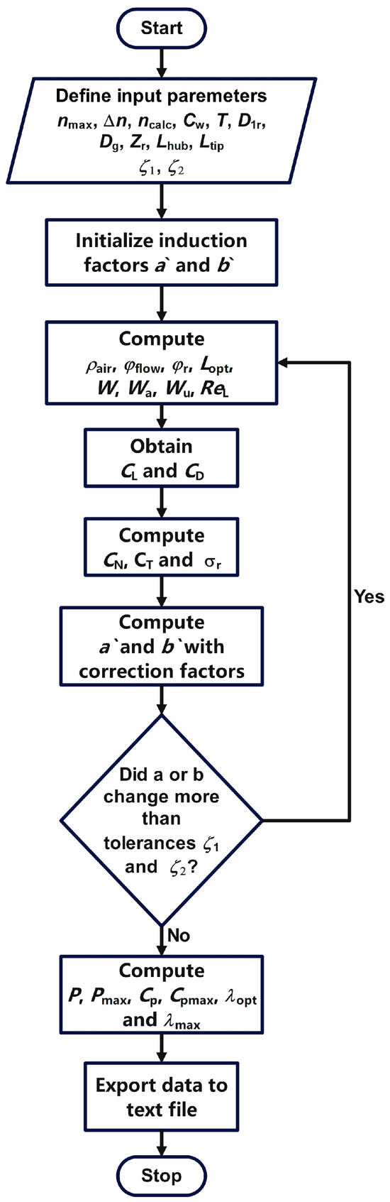
Figure 9.
Block diagram illustrating the blade optimization process.
The optimal chord length Lopt (m) for the current section is determined according to Glauert’s theory [54]:
where R (m) is the radius from the rotor’s axis of rotation to the current blade section. The values of the relative velocity W (m/s) and its projections along the rotor axis and tangent are calculated as follows [54,55,56]:
Wa,i = (1 − a‘) Cw,
Wu,i = (1 + b‘) Cw,
To calculate the aerodynamic coefficients of the airfoils CL and CD, the Reynolds number is required [57]:
The aerodynamic coefficients of the tangential and normal forces are determined by Equations (21) and (22) [54,55,56]:
With the established aerodynamic coefficients CL, the new values of the induction factors a‘new and b‘new are calculated [54,55,56]:
where σr,i defines the rotor solidity at the current section [54,55,56]:
The computational process from Equation (14) to Equation (25) is repeated until the differences between the new and old induction factors for each blade section become less than specified tolerances. Once this condition is met, the aerodynamic forces FL, FD, FT, and FN (see Figure 8), the theoretical power, Pth (W), the theoretical power coefficient Cp, th, and the theoretical tip speed ratio λth are calculated [54]:
In the above equations, (Nm) is the torque at the given blade section, (m/s) is the peripheral velocity of the rotor, and (m) are the radii of the hub and the tip sections.
The computational procedure concludes with saving the calculated parameters and the coordinates of the blade sections to a text file.
3.2. Synthesized Blade Geometry
The blade geometry was synthesized using the following input parameters: flow velocity Cw = 7 m/s, number of blades Zr = 3, rotor main diameter D1r = 1.200 m, hub diameter Dg = 0.200 m, design rotational speed ncalc = 600 min−1, number of blade sections Nsec = 9, and air temperature T = 295.15 K.
The CAD models of the blades are created using SolidWorks 2022, based on the section coordinates saved in the text files generated by the computational algorithm. The 3D geometry, the radius of each section, the blade pitch angles, and the chord lengths are shown in Figure 10.
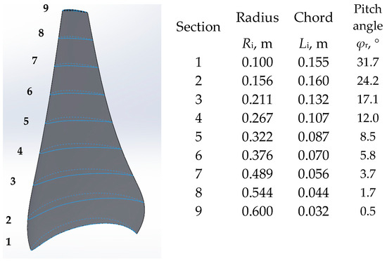
Figure 10.
Three-dimensional blade model with numbered sections and geometric data for optimized airfoil.
3.3. CFD Setup for Turbine Simulations
The CFD model used to analyze the three-bladed turbines is created using Ansys Fluent v. 2022. It consists of two domains: a stationary rectangular surrounding domain (Fluid Domain), which encompasses the airflow around the turbine, and a cylindrical rotating domain (Rotor Domain), which contains the rotor geometry. Figure 11 shows the overall dimensions, computational mesh, and boundary conditions of the surrounding domain. The cylindrical rotating domain (Figure 12) has dimensions Ø 1.5 D1r × 0.18 D1r. Its location is defined according to recommendations from the specialized literature [58,59,60]. It is positioned 60 D1r from the side and inlet boundaries of the surrounding domain and 120 D1r from the outlet. The goal is to ensure undisturbed flow in front of the turbine and allow for the free development of wake vortices behind the rotating rotor.
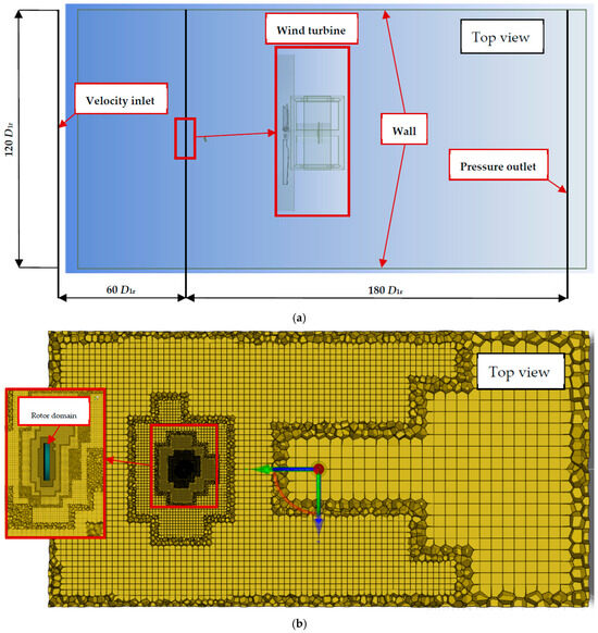
Figure 11.
(a) Overall dimensions of the surrounding domain. (b) Computational mesh.
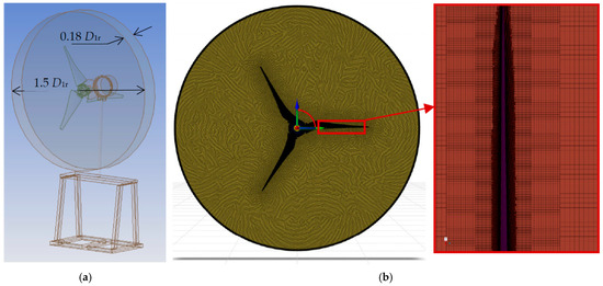
Figure 12.
(a) Overall dimensions of the rotor domain; (b) Computational mesh.
The computational mesh for both the rectangular and cylindrical domains consists of polyhedral cells. This mesh type provides better geometric quality of the cells and, consequently, higher simulation accuracy for complex geometries. In the rectangular domain, the mesh is gradually refined toward the cylindrical domain with a growth rate of 1.1 to achieve a smooth transition to the denser mesh around the rotating rotor. In the interaction zone between the airflow and the rotor, further mesh refinement is necessary to accurately capture the aerodynamic forces. The mesh parameters for both domains are summarized in Table 7 and Table 8. The achieved minimum orthogonal quality values are 0.41, 0.31, and 0.25; maximum aspect ratios of 22, 25, and 142; maximum volume ratios of 13, 15, and 1.26. These values fall within the acceptable ranges listed in Table 4.
Table 7.
Mesh parameters of the computational domains.
Table 8.
Boundary layer meshing parameters around the blades.
The boundary conditions are set in accordance with the ambient environment and the technical capabilities of the wind turbine testing laboratory at HEHT, Technical University of Sofia. At the inlet of the surrounding computational domain, a constant velocity Cw = 7 m/s is imposed, with atmospheric pressure pa = 98,200 Pa and air temperature T = 300.15 K. The walls of the surrounding domain, as well as the surfaces of the turbine and blades, are defined as no-slip walls. At the outlet of the domain, a relative pressure prel = 0 Pa is applied, corresponding to the specified atmospheric pressure.
The operating modes of the turbines are modeled using the sliding mesh technique, where the dynamic domain around the rotor rotates at a constant rotational speed. The calculations are performed using the k-ω SST, turbulence model, which is preferred in CFD simulations of turbomachinery are more accurate due to their more accurate representation of the boundary layer around the rotor blades. Preliminary values of y+ were estimated using the analytical formulas of Frank M. White. According to these estimates, to achieve y+ < 1 for a rotor with a main diameter D1r = 1.04 m and a maximum rotational speed nmax = 1000 min−1, a mesh density of approximately 8 μm in the boundary layer region is required.
4. Experimental Validation
4.1. Test Bench Description
The experiments were conducted on test bench No. 7 (Wind Turbines) in the Laboratory of Hydropower and Hydraulic Turbomachines (HEHT Lab). The bench design allows testing of turbines with both horizontal and vertical axes, with a main rotor diameter of 1.3 m. The scheme of the test bench is shown in Figure 13. The airflow is generated by an axial fan 3, driven by an asynchronous electric motor 2 with frequency control FI. The airflow is directed into an aerodynamic tube 4 with an internal diameter Dp = 1.270 m, which guides it towards the rotor of the turbine 8, after passing through a flow straightening grid 16. The flow direction can be adjusted with mechanism 1, which tilts the aerodynamic tube ±30° relative to the rotor’s axis of rotation. At the outlet, a transition 6 converts the circular cross-section to a square cross-section measuring 1.28 × 1.28 m. The flow velocity can be measured at various points in the control section in front of the rotor using a hot-wire anemometer D1, as well as inside the aerodynamic tube with a Pitot tube 15 and sensor D4. Mechanism 7 is used to position the anemometer at the desired location within the control plane. Different operating modes are simulated by the loading system, which consists of a permanent magnet electric generator 10, a rectifier 11, and a rheostat 14. The torque on the rotor shaft is measured by a torque sensor D2, while the rotational speed is measured by sensor D3. Atmospheric pressure, temperature, and air humidity are recorded with a barometer and hydrometer. The rotor is mounted on a supporting tower 12, which is fixed to the movable platform of the test bench 13. Signals from the measuring devices are processed by the control panel CS, which provides connectivity to a personal computer PC. The generator’s voltage and current are measured using a combined volt-ammeter. The rotor design allows mounting of 3, 4, 6, 8, 10, 12, or 16 blades (Zr), which can be positioned at different pitch angles ().
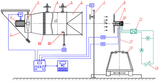
Figure 13.
Test bench schematic.
The measurement range and accuracy class of the measuring equipment (see Figure 14) are presented in Table 9, and the formulas used to calculate the main quantities are listed in Table 10.
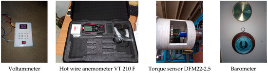
Figure 14.
Measuring equipment.
Table 9.
Range and accuracy of the measuring equipment.
Table 10.
Equations and parameters used in the calculation of turbine power curves [61,62].
4.2. Experimental Procedure
Figure 15 shows photographs of the tested rotors. The profiled blades were manufactured in separate segments using a 3D printer. The experiments were carried out at a constant average wind velocity of—Cw = 7 m/s. During the tests, the rotor’s rotational speed, atmospheric pressure, relative humidity, as well as the current and voltage of the electric generator were recorded. The operating conditions of the turbine were modeled by varying the electrical resistance in the circuit using a rheostat.
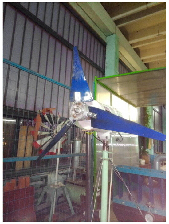
Figure 15.
Photos of the examined turbine rotor.
4.3. Data Processing
The equations used to calculate the power curves of the turbines are presented in Table 10.
In the above equations, U1r is the peripheral velocity of the rotor (m/s); Cw is the wind velocity (m/s); n is the rotor’s rotational speed (min−1); Pel is the electric power output of the generator (W); Sr is the rotor’s swept area (m2); ρair is the air density (kg/m3); Cp and λ are the power coefficient and tip speed ratio of the rotor; pa, pv, and ps are the atmospheric pressure, vapor pressure, and the saturated vapor pressure (hPa); U and I are the generator’s voltage (V) and the current (A); Mdry air and Mvapor are the molar masses of dry air and water vapor (g/mol); is the relative humidity of the air; and Rgas is the universal gas constant (J/Kmol).
4.4. Validation of CFD Results
The mesh independence study is conducted with four different meshes around the blades. Figure 16 shows the curve pattern of Cp at the optimal operation regime. The first two meshes have a finer boundary layer resolution with y = 6 and 25 μm. The third and fourth meshes are coarser, with wall distances of y = 150 and 350 μm. The difference in Cp becomes negligible for wall distances smaller than 25 μm. The results of the numerical and experimental studies of the wind turbine are presented in Figure 17 and Table 11. The black curve in Figure 17 represents the characteristics obtained from experimental testing on the laboratory test rig, the red curve corresponds to the results from CFD simulations using Ansys Fluent, the purple curve represents the predictions of the hybrid CFD-BEM method, and the blue curves show the results from the QBlade v2.09 simulation software. The highest values of the power coefficient were obtained using QBlade, reaching approximately 0.43. These results are attributed to the high L/D of the airfoils used, as calculated by XFoil. The CFD-based predictions (red curve) showed a maximum Cp of around 0.310. The hybrid CFD-BEM method closely matched the optimal operating point determined by the CFD simulations, confirming the method’s accuracy in predicting the optimal performance point of the turbine. As shown in Table 11, both the CFD and hybrid methods predicted power coefficient values that closely approach those measured experimentally in the aerodynamic wind tunnel [44] under ideal wind conditions. The differences in Cp values between the hybrid and CFD approaches, outside the optimal point, are mainly due to the high tolerance ξ2 = 0.25, used to control the convergence of the axial and tangential induction factors (a‘ and b‘). It was observed during the rotor synthesis process that lower tolerance values led to non-convergence results. The experimental results show lower Cp values (approximately 0.23). Despite the presence of a flow straightening grid, the velocity profile of the airflow in front of the rotor is still non-uniform, unlike in the CFD model. The efficiency of the generator and mechanical losses also influence the results, as the measured quantity is the electrical power output of the generator, not the mechanical power of the rotor. Nevertheless, the data from the physical experiments replicate the trend of the power curves and reach the calculated values at the optimal tip speed ratio.
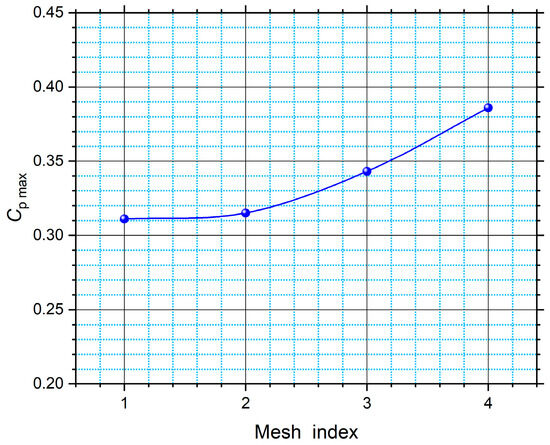
Figure 16.
Mesh independence study.
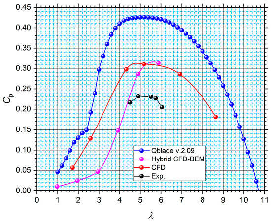
Figure 17.
Comparison of the power curves at ReD = 500,000.
Table 11.
Comparison of maximum obtained power coefficients with those from wind tunnel experiments at Reynolds number ReD = 500,000.
5. Discussion
The hybrid CFD-BEM method can predict the optimal operating mode of a small-scale wind turbine with sufficient accuracy under ideal wind conditions. The results show that the panel methods used in programs like XFoil and QBlade significantly overestimate the profile performance data (almost twice), and the turbine performance curves by up to 27.5%. This is due to the fact that these methods are based on potential flow theory and cannot accurately account for boundary layer effects and frictional losses.
By combining CFD, Ansys Workbench Design Point method and BEM rotor optimization, the hybrid methodology achieves a good balance between numerical accuracy and computational resources and time. It is suitable for both research applications and the engineering design of HAWTs operating at low Reynolds numbers. Its main contributions include, more accurate modeling of airfoil aerodynamic characteristics, and improved accuracy of the BEM method. Instead of relying on existing airfoil data, new blade shapes can be synthesized and analyzed.
One limitation of the present study is the validation only with small-scale turbines operating at low Reynolds numbers. For larger turbines, three-dimensional flow effects may have a significant impact on efficiency. However, small-scale wind turbines are widely used to supply electricity of farms, residential areas, and small households. The proposed hybrid methodology is therefore suitable for improving the efficiency of such turbines, which can enhance their broader deployment. The assessment of the on the performance of larger wind turbines will be the subject of a separate future study.
6. Conclusions
The main contributions of this study can be summarized as follows:
- The hybrid CFD-BEM methodology accurately predicts the power coefficient and optimal operating point of small-scale wind turbines.
- It provides better accuracy than commonly used IBL methods at low Reynolds numbers. It is also faster and cost-effective than modern optimization methods like ROMs and adjoint solvers. The implemented two-dimensional CFD model does not require prior training and higher computational resources;
- The validation of the presented methodology is performed on small-scale wind turbines, which are relevant for supplying electricity to farms, residential areas, and households;
- Future studies will focus on expanding this methodology for larger wind turbines, which operate at higher Reynolds numbers.
Funding
This research received no external funding.
Institutional Review Board Statement
Not applicable.
Informed Consent Statement
Not applicable.
Data Availability Statement
The data that support the findings of this study are available from the corresponding author upon reasonable request.
Acknowledgments
This research is supported by the Bulgarian Ministry of Education and Science under the second stage of the National Program “Young Scientists and Postdoctoral Students-2”.
Conflicts of Interest
The author declares no conflict of interest.
Abbreviations
The following abbreviations are used in this manuscript:
| BET | Blade Element Theory |
| BEM | Blade Element Momentum theory |
| BGA | Binary-Coded Genetic Algorithm |
| B. L. | Boundary Layer |
| CGA | Cellular Genetic Algorithm |
| CFD | Computer Fluid Dynamics |
| CS | Command System |
| DoE | Design of Experiment |
| FI | Frequency Inverter |
| GA | Genetic Algorithm |
| HAWT | Horizontal-Axis Wind Turbine |
| PC | Personal computer |
| SST | Shear Stress Transport |
| VAWT | Vertical-Axis Wind Turbine |
Nomenclatures
| Symbol | Description |
| A0 | Coefficient of Glauert Fourier series related to the camber line maximum curvature |
| A1 | Coefficient of Glauert Fourier series related to the location of the maximum curvature of the camber line |
| a‘ | Axial induction factor |
| B0 | Coefficient of Glauert Fourier series related to the maximum thickness of the blade |
| B1 | Coefficient of Glauert Fourier series related to the thickness distribution of the blade |
| b‘ | Tangential induction factor |
| CL | Lift coefficient |
| CL * | Normalized lift coefficient |
| CD | Drag coefficient |
| CN | Normal force coefficient |
| CT | Tangential force coefficient |
| Cw [m/s] | Far field velocity |
| Cp | Power coefficient |
| Cp,init | Power coefficient before the optimization |
| Cp,max | Maximum power coefficient |
| Cp,opt | Power coefficient after the optimization |
| D1r [m] | Main diameter of the turbine |
| Dp [m] | Inner diameter of the aerodynamic tube |
| [N] | Drag force |
| [N] | Lift force |
| [N] | Normal force |
| [N] | Tangential force |
| [m2/s] | Total bound circulation from the leading edge up to the position defined by the angle θ |
| [m/s] | Vortex sheet strength per unit length |
| I [A] | Current |
| L/D | |
| Lr [m] | Chord length |
| Lopt [m] | Optimal chord length |
| Lhub [m] | Chord length at the hub |
| Ltip [m] | Chord length at the tip |
| Mdry air [g/mol] | Molar mass of dry air |
| Mvapor [g/mol] | Molar mass of vapor |
| Nsec | Number of blade sections used in the BEM calculation |
| n [min−1] | Rotational speed |
| Δn [min−1] | Rotational speed increment step |
| ncalc [min−1] | Design rotational speed |
| nmax [min−1] | Maximum rotational speed |
| P [W] | Mechanical power |
| Pel [W] | Electric power |
| pa [hPa] | Atmospheric pressure |
| pv [hPa] | Vapor pressure of water |
| ps [hPa] | Saturation pressure of water |
| ) [m] | |
| ) [m2/s] | Source strength per unit length, derived from the thickness distribution. |
| Rgas [J/Kmol] | Ideal gas constant |
| R [m] | Radius at a specific blade section |
| Rhub [m] | Hub radius |
| Rtip [m] | Tip radius |
| Re | Radius at a specific blade section |
| Reynolds number based on rotor diameter | |
| Reynolds number based on airfoil chord length | |
| Sr [m2] | Rotor flow area |
| T [K] | Air temperature |
| Tτ [Nm] | Torque of the rotor |
| U [m/s] | Peripheral speed of the rotor |
| U1r [m/s] | Peripheral speed at rotor tip |
| Uel [V] | Voltage |
| [m/s] | The x-component of the velocity induced at given point by a distribution of singularities |
| ut [m/s] | Tangential velocity component on the streamlined surface |
| [m/s] | The x-component of the velocity induced by thickness source distribution |
| [m/s] | The y-component of the velocity induced at given point by a distribution of singularities |
| [m/s] | The y-component of the velocity induced by thickness source distribution |
| W [m/s] | Relative velocity |
| Wa [m/s] | Axial component of relative velocity |
| Wu [m/s] | Tangential component of the relative velocity |
| X | Dimensionless coordinate in horizontal direction |
| x [m] | X-coordinate of the point where velocity is evaluated |
| x‘ [m] | X-coordinate of the singularity point where the vortex or source is located |
| Y | Dimensionless coordinate in vertical direction |
| y [m] | Y-coordinate of the point where velocity is evaluated |
| y‘ [m] | Y-coordinate of the singularity point where the vortex or source is located |
| y+ | Dimensionless wall distance |
| ywall [m] | Normal distance from the streamlined surface |
| Zr | Number of blades |
| α [rad] | Angle of attack |
| αopt [rad] | Optimal angle of attack |
| θ [rad] | An angular coordinate that maps points along the airfoil contour |
| Tip speed ratio | |
| opt | Optimal tip speed ratio |
| [m2/s] | Kinematic viscosity of air |
| ξ1 | Tolerance for convergence in the calculation of induction factors in the optimal regime |
| ξ2 | Tolerance for convergence in the calculation of induction factors outside the optimal regime |
| ρair [kg/m3] | Density of air |
| Rotor solidity | |
| φr [rad] | Pitch angle at a specific blade section |
| φflow [rad] | Flow angle at a specific blade section |
| Relative humidity of the air | |
| ωcalc [rad/s] | Design angular velocity |
References
- Sultan, K.; Elshabli, A.; Kashbour, A.; Atega, S.B. Performance assessment of the vortex panel method. Libyan J. Sci. Technol. 2019, 9, 122–128. [Google Scholar] [CrossRef]
- Cox, C. Linear Strength Vortex Panel Method for a Two Element Airfoil. Senior Bachelor’s Thesis, California Polytechnic State University, San Luis Obispo, CA, USA, 2011. Available online: https://digitalcommons.calpoly.edu/aerosp/28/ (accessed on 1 July 2025).
- Bristow, D. A New Surface Singulatity Method for Multi-Element Airfoil Analysis and Design. In Proceedings of the 14th Aerospace Sciences Meeting, Washington, DC, USA, 26–28 January 1976. [Google Scholar] [CrossRef]
- Bottai, A.; Jonson, L.; Campbell, R. Singularity Based Method for Small Peturbation Unsteady Aerodynamics Using Higher Fidelity Steady State Pressure Profiles. In Proceedings of the ASME 2023 International Mechanical Engineering Congress and Exposition, New Orleans, LA, USA, 29 October–2 November 2023. [Google Scholar] [CrossRef]
- Sørensen, J.; Ramos-García, N.; Okulov, V. Analysis and Validation of Glauert Rotor Design. J. Phys. Conf. Ser. 2022, 2265, 032047. [Google Scholar] [CrossRef]
- Abedi, H. Development of Vortex Filament Method for Aerodynamic Loads on Rotor Blades. Licentiate of Engineering. Bachelor’s Thesis, Chalmers University of Technology, Gothenburg, Sweden, 2013. Available online: https://www.tfd.chalmers.se/~lada/postscript_files/Licentiate_thesis_Hamid.pdf (accessed on 26 June 2025).
- Queipo, N.; Haftka, R.; Shyy, W.; Goel, T.; Vaidyanathan, R.; Tucker, P. Surrogate-based analysis and optimization. Prog. Aerosp. Sci. 2005, 41, 1–28. [Google Scholar] [CrossRef]
- Han, Z.; Zhang, K. Real-World Applications of Genetic Algorithms; IntechOpen: London, UK, 2012; pp. 333–362. [Google Scholar] [CrossRef]
- Agrawal, R.; Bose, S.; Griffin, K.; Moin, P. An extension of Thwaties’ method for turbulent boundary layers. Flow 2024, 4, E25. [Google Scholar] [CrossRef]
- Mason, W. Aerodynamic Calculation Methods for Programmable Calculators & Personal Computers; Huntington: New York, NY, USA, 1981; Available online: https://archive.aoe.vt.edu/mason/Mason_f/AerocalPak4.pdf (accessed on 29 June 2025).
- Hwang, P.; Wu, J.; Chang, Y. Optimization Based on Computational Fluid Dynamics and Machine Learning for the Performance of Diffuser-Augmented Wind Turbines with Inlet Shrouds. Sustainability 2024, 16, 3648. [Google Scholar] [CrossRef]
- Kenway, G.; Mader, C.; He, P.; Martins, J. Effective adjoint approaches for computational fluid dynamics. Prog. Aerosp. Sci. 2019, 110, 100542. [Google Scholar] [CrossRef]
- Amoignon, O. Adjoint-Based Aerodynamic Shape Optimization. Ph.D. Thesis, Uppsala University, Uppsala, Sweden, 2003. Licentiate of Technology in Numerical Analysis. [Google Scholar]
- Dhert, T.; Ashuri, T.; Martins, J. Aerodynamic Shape Optimization of Wind Turbine Blades Using a Reynolds-Averaged Navier-Stokes Model and an Adjoint Method. Wind Energy 2017, 20, 909–926. [Google Scholar] [CrossRef]
- Vardhan, H.; Hyde, D.; Timalsina, U.; Volgyesi, P.; Sztipanovits, J. Sample-efficient and surrogate-based design optimizxation of underwater vehicle hulls. Ocean Eng. 2024, 311, 118777. [Google Scholar] [CrossRef]
- Saalfield, B.; Rutten, M.; Saalfiield, S.; Kunemund, J. Improved Mesh Morphing Based on Radial Basis Functions. In Proceedings of the 6th European Congress on Computational Methods in Applied Sciences and Engineering (ECCOMAS 2012), Vienna, Austria, 10–14 September 2012; Available online: https://www.researchgate.net/publication/225026002_Improved_Mesh_Morphing_Based_on_Radial_Basis_Functions (accessed on 18 July 2025).
- Airfoil Tools. Available online: http://airfoiltools.com/ (accessed on 16 July 2025).
- Schmitz, S.; Maniaci, C. Methodology to determine a tip-loss factor for highly loaded wind turbines. AIAA 2017, 55, 341–351. [Google Scholar] [CrossRef]
- Zhao, D.; Han, N.; Goh, E.; Cater, J.; Reinecke, A. Wind Turbines and Aerodynamics Energy Harvesters, 1st ed.; Academic Press: Cambridge, MA, USA, 2019; pp. 373–400. [Google Scholar]
- Drela, M. XFOIL: An Analysis and Design System for Low Reynolds Number Airfoils. In Low Reynolds Number Aerodynamics; Springer: Berlin/Heidelberg, Germany, 1989; Volume 54, pp. 1–12. [Google Scholar] [CrossRef]
- Marten, D.; Wendler, J.; Pechivanoglou, G.; Nayeri, C.; Paschereit, C. Qblade: An open source tool for design and simulation of horizontal and vertical axis Wind turbines. Int. J. Emerg. Technol. Adv. Eng. 2013, 3, 264–269. [Google Scholar]
- PROPAN—Propeller Panel Code. Available online: https://www.researchgate.net/publication/356556813_PROPAN_-_Propeller_Panel_Code (accessed on 15 June 2025).
- Eppler, R. Airfoil Design and Data; Springer: Berlin/Heidelberg, Germany, 1990. [Google Scholar]
- Romani, G.; Grande, E.; Avallone, F.; Ragni, D.; Casalino, D. Performance and Noise Prediction of Low-Reynolds Number Propellers Using the Lattice-Boltzmann Method. Aerosp. Sci. Technol. 2022, 125, 107086. [Google Scholar] [CrossRef]
- Klose, B.F.; Spedding, G.R.; Jacobs, G.B. Flow Separation, Instability and Transition to Turbulence on a Cambered Airfoil at Reynolds Number 20000. J. Fluid Mech. 2025, 1009, A9. [Google Scholar] [CrossRef]
- Cantwell, B.J.; Bilgin, E.; Needels, J.T. A New Boundary Layer Integral Method Based on the Universal Velocity Profile. Phys. Fluids 2022, 34, 075130. [Google Scholar] [CrossRef]
- Rapp, B. Microfluidics: Modelling, Mechanics and Mathematics, 1st ed.; Elsevier: Amsterdam, The Netherlands, 2016; pp. 273–289. [Google Scholar]
- Quarona, E. Design Loading Optimization of a Horizontal Axis Turbine with Lifting Line and Panel Methods. Master’s Thesis, Instituto Superior Técnico, Universidade de Lisboa, Lisboa, Portugal, 2019. [Google Scholar]
- Goates, C.D.; Hunsaker, D.F. Practical Implementation of a General Numerical Lifting-Line Method. In Proceedings of the AIAA Scitech 2021 Forum, Virtual, 11–21 January 2021; American Institute of Aeronautics and Astronautics: Reston, VA, USA. [Google Scholar] [CrossRef]
- Koc, E.; Gunel, O.; Yavuz, T. Comparison of QBlade and CFD Results for Small-Scaled Horizontal Axis Wind Turbine Analysis. In Proceedings of the 2016 IEEE International Conference on Renewable Energy Research and Applications (ICRERA), Birmingham, UK, 20–23 November 2016; IEEE: New York, NY, USA, 2016; pp. 204–209. [Google Scholar] [CrossRef]
- Pourrajabian, A.; Dehghan, M.; Rahgozar, S. Genetic Algorithms for the Design and Optimization of Horizontal Axis Wind Turbine (HAWT) Blades: A Continuous Approach or a Binary One? Sustain. Energy Technol. Assess. 2021, 44, 101022. [Google Scholar] [CrossRef]
- Poole, S.; Phillips, R. Optimization of a Mini H.A.W.T. Blade to Increase Energy Yield during Short Duration Wind Variations. J. New Gener. Sci. 2016, 14, 47–59. [Google Scholar]
- Bekkai, R.; Mdouki, R.; Laouar, R. Aerodynamic Optimization of 3D Micro HAWT Blade via RSM. J. Appl. Fluid Mech. 2025, 18, 504–517. [Google Scholar] [CrossRef]
- Ansys Fluent Software. Available online: https://www.ansys.com/products/fluids/ansys-fluent (accessed on 23 July 2025).
- Radi, J.; Sierra-García, J.; Santos, M.; Armenta-Déu, C.; Djebli, A. Metaheuristic Optimization of Wind Turbine Airfoils with Maximum-Thickness and Angle-of-Attack Constraints. Energies 2024, 17, 6440. [Google Scholar] [CrossRef]
- Boudis, A.; Hamane, D.; Guerri, O.; Bayeul-Laine, A. Airfoil Shape Optimization of a Horizontal Axis Wind Turbine Blade Using a Discrete Adjoint Solver. J. Appl. Fluid Mech. 2023, 16, 724–738. [Google Scholar] [CrossRef]
- Kriswanto; Setiawan, M.; Al-Janan, D.; Naryanato, R.; Roziquin, A.; Firmansyah, H.; Setiadi, R.; Darsono, F.; Setiyawan, A.; Jamari; et al. Power Optimization of The Horizontal Axis Wind Turbine Capacity of 1 MW on Various Parameters of The Airfoil, an Angle of Attack, and a Pitch Angle. J. Adv. Res. Fluid Mech. Therm. Sci. 2023, 103, 141–156. [Google Scholar] [CrossRef]
- Antony, J. Taguchi or Classical Design of Experiments: A Perspective from a Practitioner. Sens. Rev. 2006, 26, 227–230. [Google Scholar] [CrossRef]
- Mohammadi, M.; Mohammadi, A.; Farahat, S. A New Method for Horizontal Axis Wind Turbine (HAWT) Blade Optimization. Int. J. Renew. Energy Dev. 2016, 5, 1–8. [Google Scholar] [CrossRef]
- Al-Abadi, A.; Ertunç, Ö.; Beyer, F.; Delgado, A. Torque-Matched Aerodynamic Shape Optimization of HAWT Rotor. J. Phys. Conf. Ser. 2014, 555, 012003. [Google Scholar] [CrossRef]
- Shen, X.; Zhu, X.; Du, Z. Optimization of Wind Turbine Blades Using Lifting Surface Method and Genetic Algorithm. In Proceedings of the ASME 2011 Turbo Expo: Turbine Technical Conference and Exposition, Vancouver, BC, Canada, 6–10 June 2011; pp. 841–847. [Google Scholar]
- Lee, K.-J.; Hoshino, T.; Lee, J.-H. A Lifting Surface Optimization Method for the Design of Marine Propeller Blades. Ocean. Eng. 2014, 88, 472–479. [Google Scholar] [CrossRef]
- Umar, D.A.; Yaw, C.T.; Koh, S.P.; Tiong, S.K.; Alkahtani, A.A.; Yusaf, T. Design and Optimization of a Small-Scale Horizontal Axis Wind Turbine Blade for Energy Harvesting at Low Wind Profile Areas. Energies 2022, 15, 3033. [Google Scholar] [CrossRef]
- Devlin, K.; Miller, M. High Reynolds Number Wind Turbine Testing in the Compressed Air Wind Tunnel. In Proceedings of the 2024 Regional Student Conferences; American Institute of Aeronautics and Astronautics AIAA: Reston, VA, USA, 2024. [Google Scholar] [CrossRef]
- Cunningham, J. Field Testing the Effects of Low Reynolds Number on the Power Performance of the Cal Poly Wind Power Research Center Small Wind Turbine. Master’s Thesis, California Polytechnic State University, San Luis Obispo, CA, USA, 2020. Available online: https://digitalcommons.calpoly.edu/theses/2249 (accessed on 16 July 2025).
- Peters, N.; Silva, C.; Ekaterinaris, J. A Data-Driven Reduced-Order Model for Rotor Optimization. Wind Energ. Sci. 2023, 8, 1201–1223. [Google Scholar] [CrossRef]
- Popov, M. Hydrodynamics, 1st ed.; State Publishing House “Technika”: Sofia, Bulgaria, 1973. [Google Scholar]
- Mohamed, O.; Ibrahim, A.; Etman, E.; Abdelfatah, A.; Elbaz, A. Numerical Investigation of Darrieus Wind Turbine with Slotted Airfoil Blades. Energy Convers. Manag. X 2020, 5, 100026. [Google Scholar] [CrossRef]
- Adam, N.; Attia, O.; Al-Sulttani, A.; Mahmood, H.; As’arry, A.; Md Rezali, K. Numerical Analysis for Solar Panel Subjected with an External Force to Overcome Adhesive Force in Desert Areas. CFD Lett. 2020, 12, 60–75. [Google Scholar] [CrossRef]
- ANSYS Inc. ANSYS Fluent User’s Guide, Version 2022; ANSYS Inc.: Canonsburg, PA, USA, 2022. [Google Scholar]
- Durmuş, S.; Ulutaş, A. Numerical Analysis of NACA 6409 and Eppler 423 Airfoils. J. Polytech. 2023, 26, 39–47. [Google Scholar] [CrossRef]
- White, M. Viscous Fluid Flow, 3rd ed.; McGraw-Hill: New York, NY, USA, 2006. [Google Scholar]
- Menter, F.R. Zonal Two Equation Kappa-Omega Turbulence Models for Aerodynamic Flows. In Proceedings of the AIAA Fluid Dynamics Conference (No. AIAA Paper 93-2906), Orlando, FL, USA, 6–9 July 1993; AIAA: Reston, VA, USA, 1993. [Google Scholar]
- Hansen, M. Aerodynamics of Wind Turbines, 3rd ed.; Routledge: Oxford, UK, 2015. [Google Scholar]
- Manwell, J.F.; McGowan, J.G.; Rogers, A.L. Wind Energy Explained: Theory, Design and Application, 2nd ed.; Wiley: Chichester, UK, 2009. [Google Scholar]
- Burton, T.; Sharpe, D.; Jenkins, N.; Bossanyi, E. Wind Energy Handbook, 2nd ed.; Wiley: Chichester, UK, 2011. [Google Scholar]
- Saldana, M.; Gallegos, S.; Gálvez, E.; Castillo, J.; Salinas-Rodríguez, E.; Cerecedo-Sáenz, E.; Hernández-Ávila, J.; Navarra, A.; Toro, N. The Reynolds Number: A Journey from Its Origin to Modern Applications. Fluids 2024, 9, 299. [Google Scholar] [CrossRef]
- Wußow, S.; Sitzki, L.; Hahm, T. 3D-Simulation of the Turbulent Wake behind a Wind Turbine. J. Phys. Conf. Ser. 2007, 75, 012033. [Google Scholar] [CrossRef]
- Kao, J.-H. Developing the Process in Matching a Wind Turbine System to Attain Optimal Performance. Adv. Mech. Eng. 2016, 8, 1687814016674697. [Google Scholar] [CrossRef]
- Rezaeiha, A.; Montazeri, H.; Blocken, B. Towards Accurate CFD Simulations of Vertical Axis Wind Turbines at Different Tip Speed Ratios and Solidities: Guidelines for Azimuthal Increment, Domain Size and Convergence. Energy Convers. Manag. 2018, 156, 301–316. [Google Scholar] [CrossRef]
- Tsilingiris, P. Thermophysical and Transport Properties of Humid Air at Temperature Range between 0 and 100 °C. Energy Convers. Manag. 2008, 49, 1098–1110. [Google Scholar] [CrossRef]
- Alduchov, O.; Eskridge, R. Improved Magnus Form Approximation of Saturation Vapor Pressure. J. Appl. Meteor. 1996, 35, 601–609. [Google Scholar] [CrossRef]


Disclaimer/Publisher’s Note: The statements, opinions and data contained in all publications are solely those of the individual author(s) and contributor(s) and not of MDPI and/or the editor(s). MDPI and/or the editor(s) disclaim responsibility for any injury to people or property resulting from any ideas, methods, instructions or products referred to in the content. |
© 2025 by the author. Licensee MDPI, Basel, Switzerland. This article is an open access article distributed under the terms and conditions of the Creative Commons Attribution (CC BY) license (https://creativecommons.org/licenses/by/4.0/).