Ten-Year Analysis of Mediterranean Coastal Wind Profiles Using Remote Sensing and In Situ Measurements

Abstract

Accurate near-surface wind speed and direction measurements are crucial for validating atmospheric models, especially for the purpose of adequately assessing the interactions between the surface and wind, which in turn results in characteristic vertical profiles. Coastal regions pose unique challenges due to the discontinuity between land and sea and the complex interplay of atmospheric stability, topography, and boundary/layer dynamics. This study focuses on a unique database of wind profiles collected over several years at a World Meteorological Organization—Global Atmosphere Watch (WMO/GAW) coastal site in the southern Italian region of Calabria (Lamezia Terme, code: LMT). By leveraging remote sensing technologies, including wind lidar combined with in situ measurements, this work comprehensively analyzes wind circulation at low altitudes in the narrowest point of the entire Italian peninsula. Seasonal, daily, and hourly wind profiles at multiple heights are analyzed, highlighting the patterns and variations induced by land–sea interactions. A case study integrating Synthetic Aperture Radar (SAR) satellite images and in situ observations demonstrates the importance of multi-sensor approaches in capturing wind dynamics and validating model simulations. Data analyses demonstrate the occurrence of extreme events during the winter and spring seasons, linked to synoptic flows; fall seasons have variable patterns, while during the summer, low-speed winds and breeze regimes tend to prevail. The prevailing circulation is of a westerly nature, in accordance with other studies on large-scale flows.

1. Introduction

Atmospheric boundary/layer dynamics govern the exchange of momentum, heat, and moisture near the Earth’s surface, shaping weather systems, driving pollution dispersion, and determining renewable energy potential [1,2,3,4]. Coastal areas, such as Italy’s Mediterranean coastline, amplify these complexities due to dynamic land–sea interactions, topographical influences, and synoptic-scale circulations, resulting in wind behaviors that challenge predictions and enhanced modeling [5].

Over the past two decades, advances in remote sensing technologies—such as Doppler lidar, wind lidar, and Synthetic Aperture Radar (SAR)—have revolutionized wind profiling, enabling high-resolution vertical and spatial measurements of wind speed, direction, and turbulence [6,7]. The Mediterranean Basin, with its narrow peninsulas, steep orography, and climatic sensitivity, serves as a critical region for studying boundary/layer processes, where phenomena like land–sea breezes, nocturnal low-level jets, and turbulence regimes dominate local meteorology and air quality [8,9,10,11]. These tools, complemented by ground-based sodars and anemometers, have unveiled intricate details of coastal atmospheric dynamics, including diurnal breeze transitions, shear-driven turbulence, and orographic modulation of airflow [12,13,14]. For instance, SAR imaging has mapped spatial wind gradients across land–sea interfaces, while lidar systems have resolved nocturnal jets critical for dust transport and pollutant dispersion [15,16]. Another key aspect characterizing the implementation of advanced methodologies is a more detailed understanding of seasonal and interannual patterns in wind speed, direction, and turbulence, including the interplay of synoptic-scale systems (e.g., mistral winds) and local circulations (e.g., slope flows) [17,18]. Water vapor transport is also a key factor in driving these mechanisms. In the context of the Mediterranean Basin, this mechanism was also investigated, revealing its role in convective activity and precipitation processes [19].

A detailed evaluation of the dynamics of downslope winds and gravity-driven circulations in mountainous coastal areas, emphasizing the connection between turbulence, topography, and extreme weather phenomena; these findings directly apply to understanding Italy’s coastal atmospheric dynamics, where wind profiling is crucial in renewable energy planning and disaster mitigation [20].

Furthermore, recent research by Hagay and Brenner (2021) [21] expanded on the interaction of wind circulation with sea surface temperatures, emphasizing how thermal gradients influence wind speed and direction. These interactions are especially pronounced in the Mediterranean, where seasonal changes in sea surface temperatures significantly affect atmospheric conditions. They also found that such interactions are critical for forecasting storm development and mitigating weather-related risks.

Coastal vegetation and land use in modifying wind circulation patterns may play a role in driving wind and climate variability in these environments [22]; natural and anthropogenic factors can alter local meteorological conditions, providing a holistic understanding of the atmospheric dynamics in coastal zones [22]. The role of mesoscale circulation in driving localized weather extremes has also been investigated in the literature. By utilizing high-resolution numerical models, the interactions between mesoscale wind systems and large-scale atmospheric processes became a prominent niche in the field of Atmospheric Sciences, contributing to the broader understanding of extreme weather formation in coastal and mountainous regions [23].

As ecosystems become more exposed to anthropic activities and significant perturbations to shorelines occur, the impact of urbanization on coastal wind dynamics has also become the subject of research in the literature [24], highlighting how built environments influence airflow patterns and turbulence. Similar findings are particularly relevant to regions like Italy’s Mediterranean coastline, where urban expansion continues to reshape the coastal landscape despite the introduction of ad hoc regulations meant to mitigate these effects. The study provides actionable insights for urban planners aiming to minimize adverse environmental impacts.

Finally, Stathopoulos et al. (2020) [25] explored the implications of wind circulation studies for offshore renewable energy projects. Their research emphasized the importance of accurate wind profiling in optimizing the placement and efficiency of wind turbines. These findings directly relate to Italy’s efforts to expand renewable energy infrastructure along its Mediterranean coastline. It is also worth mentioning that orographic barriers, such as Sardinia and Corsica, alter wind trajectories and moisture transport in the Mediterranean, affecting localized precipitation patterns [26]. Lastly, Zhou et al. (2019) [27] evaluated the role of turbulent orographic form drag on wind and precipitation, emphasizing its impact on atmospheric water vapor transport over mountainous regions. These studies highlight the complex nature of wind circulation research in coastal and mountainous regions, emphasizing the importance of integrating diverse factors such as orographic influences, water vapor transport, thermal gradients, and human impacts. This approach enables the development of comprehensive models to predict and mitigate extreme weather events, which are crucial for sustainable development and disaster resilience in regions like Italy’s Mediterranean coastline. Incorporating wind profiling technologies has further enhanced our understanding of low-altitude wind circulation by capturing fine-scale atmospheric turbulence and vertical flows. These profiles improve boundary/layer dynamics modeling, benefiting climate studies, energy system optimization, and disaster preparedness.

Advances in this field of research clearly point in the direction of implementing in situ measurements as vital tools towards an adequate characterization of specific areas. Moreso, the measurements have to account for prolonged periods of time, in the order of several years, to evaluate possible tendencies and better discriminate sporadic outliers from indicators of ongoing changes in climate patterns. In this study, more than one decade of measurements are characterized and described in a regional coastal World Meteorological Organization—Global Atmosphere Watch (WMO/GAW) in Calabria, Southern Italy, namely the Lamezia Terme (code: LMT) site. The findings presented in this study constitute the evaluation of the longest time series ever performed at the observation site and provide a state-of-the-art understanding of surface and near-surface circulation in the narrowest point of the Italian peninsula. With a growing number of works showing a close relationship between local wind patterns and the concentrations of aerosols, greenhouse gases (GHGs) and pollutants posing hazards for the environment and human health [28,29,30,31], this study shifts toward the direction of providing more reliable fundaments to hypotheses on the local interplay between wind circulation and gas/aerosol concentrations. This approach underlines the importance of surface and near-surface wind pattern characterization in fields such as air pollution control, in addition to the assessment of renewable energy exploitation in a given area.

This article details the data acquisition process at the Lamezia Terme observatory’s experimental site and the geomorphological features of the Catanzaro isthmus in Section 2. In Section 3, the instruments and methodologies used in this study are reported. Section 4 and Section 5 are focused on the results and discussion, respectively. Section 6 concludes the study.

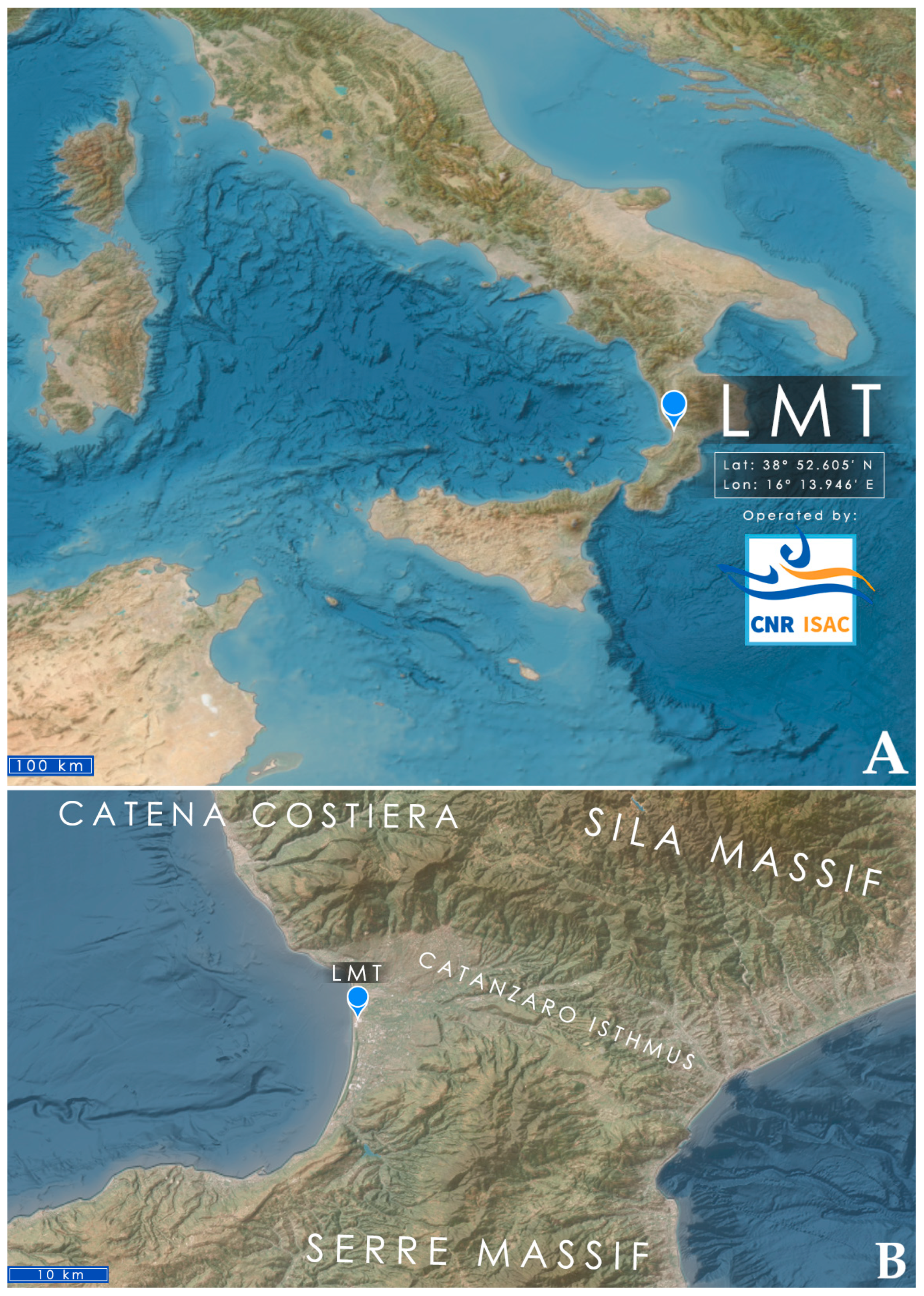
2. Characteristics of the LMT Site

The Lamezia Terme (code: LMT; Lat: 38°52.605′ N; Lon: 16°13.946′ E; Alt: 6 m ASL) observation site is located in the Southern Italian region of Calabria (Figure 1A), 600 m from the Tyrrhenian coast of the region. The station, which is part of the WMO/GAW (World Meteorological Organization—Global Atmosphere Watch) network, is fully operated by the National Research Council of Italy—Institute of Atmospheric Sciences and Climate (CNR-ISAC). LMT started data-gathering operations on atmospheric greenhouse gases and aerosols in 2015 [28,29,30,31]. However, a number of meteorological parameters, such as those evaluated in the present work, had been subject to measurements as early as 2013. A short summer campaign in 2009 allowed for the preliminary characterization of local wind circulation prior to the main LMT data-gathering operations [8,32,33]. These early findings also included a preliminary characterization of PBLH (Planetary Boundary Layer Height) variability at the site, which was later expanded during a summer 2024 campaign aimed at testing the correlation between meteorological parameters, greenhouse gases, aerosols, and particulate matter [34].

LMT’s location marks the westernmost sector of the Catanzaro isthmus, which is the narrowest point in the entire Italian peninsula (≈32 km between the Tyrrhenian/western and Ionian/eastern coasts of the region) (Figure 1B). The isthmus has a peculiar orographic configuration, bounded by the Sila Massif (north), Catena Costiera (Coastal Chain, northwest), and the Serre Massif (south). This configuration has a strong influence on surface and near-surface wind circulation, as evidenced by a number of early works on the area. Federico et al. (2010a) [35] showed the importance of breeze regimes as a key factor of local circulation and climate; seasonal variations were also observed, including minor changes in wind directions. A main W-WSW/NE-ENE axis is present, resulting from wind being channeled through the isthmus; however, when the 850 hPa layer is considered, a prevailing northwestern direction is reported, which is in accordance with large-scale flows of the area. Federico et al. (2010b) [5] evaluated two years of data to further characterize local wind circulation and wind regimes. Between November and February, diurnal wind circulation is connected to large-scale forcing. The March–October period is characterized by diurnal breezes, which result from a combination of local and large-scale flows. Nighttime flows are related to nocturnal breeze regimes.

Figure 1. (A): Modified EMODnet digital elevation model (DEM) [36] of Central and Southern Italy, with a focus on LMT’s coordinates, location, and operating institution. (B): Additional details of the Catanzaro isthmus, its local geomorphology, and the three mountain ranges bounding the plain where LMT is located.

Figure 1. (A): Modified EMODnet digital elevation model (DEM) [36] of Central and Southern Italy, with a focus on LMT’s coordinates, location, and operating institution. (B): Additional details of the Catanzaro isthmus, its local geomorphology, and the three mountain ranges bounding the plain where LMT is located.

In D’Amico et al.’s study (2024e) [34], in addition to new data on PBLH variability at LMT, the importance of wind regime categorization emerged. Due to the peculiar wind circulation at the site, a number of parameters were proven to be affected by breeze or synoptic regimes, which reflected distinct correlations between anthropogenic pollution and air mass transport. As additional evidence on the importance of local wind patterns, it is worth mentioning that the Lamezia Terme International Airport (IATA: SUF; ICAO: LICA), located 3 km north from the observatory, has a 100/280° N runway (RWY) orientation causing local air traffic to be influenced by the same wind patterns observed at LMT.

The local orographic configuration, which is responsible for channeling winds through the isthmus, is the result of a number of geodynamical processes. In the early Quaternary period (≈2.5 million years ago, mya), the isthmus was a tidal strait, as confirmed by outcrops of 2D and 3D dunes in the central area of the isthmus itself [37,38,39].

Transgression and regression cycles, primarily regulated by the Calabrian uplift [40,41,42,43] and major variations in sea levels, such as those induced by glacial/interglacial periods [41,42,43,44], have ultimately cut off water circulation in the strait, leading to the present-day configuration.

The entire region of Calabria is part of the much larger CPA (Calabria–Peloritani Arc), also including the northeastern areas of Sicily [45,46,47]. The arc rifted apart from continental Europe following the Mesozoic spreading of the Alpine Tethys domains and started drifting towards the southeast, ultimately colliding with the Italian peninsula [48]. The drift is still active [49,50] and is responsible for the opening of the Tyrrhenian Sea at high rates; specifically, the Marsili basin opening rate in the central Tyrrhenian has been estimated to be one of the fastest observed rates in recent geological history [51].

The Aeolian Arc of volcanoes in the Tyrrhenian Sea, which includes active volcanic islands and seamounts, is also an indicator of active geodynamics linked to the southwestward migration of CPA [52,53,54,55]. With the Stromboli volcano being located only 88 km W–SW from LMT, the observation site is deemed to be subject to sporadic volcanic outputs [56], thus contributing to the peculiarity of LMT’s location in the Mediterranean.

Intense faulting, driven by extensional tectonics [57,58,59], has completely reshaped the local geomorphology: the Catanzaro isthmus is now effectively delimited by fault systems and three mountain ranges. Differences in elevation between the plain and nearby mountains in the order of ≈1250 m. Overall, various fault systems now characterize the Calabrian region [60,61], with the Lamezia Terme–Catanzaro fault line showing a well-defined E-W orientation bounding the Catanzaro isthmus on the northern sector [62]. The southern sector is bounded by W-NW/E-SE faulting related to the Curinga–Girifalco line [62,63,64]. The area is seismically active, with many of the strongest earthquakes in recorded Italian history (between 1000 and 2024 A.D.) taking place within a ≈20 km radius from the current location of LMT (three out of ten earthquakes with Mw ≥ 6.95) [65,66]. The present-day shoreline, in addition to the short distance between two seas and tectonics-driven geomorphology, therefore results in a unique environment for surface and near-surface wind circulation in the Italian peninsula.

3. Instruments and Methodologies

At LMT, measurements of wind speed (WS) and wind direction (WD) were performed using a Vaisala WXT520 (Vantaa, Finland) 10 m above ground level (AGL). This instrument is frequently used to perform measurements of wind parameters and other key data (such as temperature, relative humidity, rainfall, and hail) [67]. The WXT520 relies on WINDCAP sensor technology for wind measurements: specifically, the WINDCAP is composed of an array of three ultrasonic transducers. The transducers are equally spaced on a horizontal plane at the top of the weather station. WS and WD are calculated by measuring the time required for ultrasound pulses to travel from each of the transducers to the other two; WINDCAP therefore measures six (two per transducer) transit times in both directions in the array, which is affected by ambient wind speed over the path of ultrasonic pulses. Pulses traveling upwind have a longer transit time compared to their downwind counterparts. In the case of no wind speed (0 m/s), the reverse and forward transit times would be the same.

The WXT520 provides an option to select scalar speed in meters per second (m/s), knots (kt), miles per hour (mph), and kilometers per hour (km/h). At both LMT and in other stations across the network, wind speed is reported in m/s. Wind direction is reported in degrees° N. The instrument has an operating range for wind speed between 0 and 60 m/s, with a response time of 0.25 s and an accuracy of ±3% at 10 m/s; in the case of wind direction, the accuracy is ±3.0°, and the output resolution is 1°. For the purpose of this work, hourly averaged data and their respective standard deviations were calculated.

Vertical profiles were measured via a ZephIR 300 wind lidar device (ZX Lidars, Malvern, UK), which is a homodyne coherent detection continuous-wave (CW)-focusing wind lidar [68]. At LMT, results from the same instruments were the subject of previous works on the preliminary characterization of vertical wind profiles in the area [8,69]. The instrument measures wind via detecting the Doppler shift in the infrared laser, which is scattered by particulates suspended in the atmosphere (e.g., aerosols) and subject to transport [70]. Changes in wind speed over the analyzed vertical profiles are detected by the instrument as slight frequency variations. The ZephIR is set to measure wind speeds over specific altitude thresholds, which can be configured by the user. At LMT, the following thresholds were set: 300 m, 250 m, 200 m, 150 m, 120 m, 100 m, 80 m, 60 m, 20 m, and 10 m. This multi-layer measurement enables VAD (Velocity Azimuth Display) scanning, which is performed via laser beam emission at a constant elevation angle while the azimuth angle changes depending on each altitude threshold [71]. A rotating deflector prism can therefore achieve conical scanning, as each azimuth angle is linked to a given wind component (radial speed) in a specific direction of the emitted beam. Multiple consecutive measurements over a circle allow for the velocity vector to be calculated at the center of the projected cone for each altitude threshold [72,73]. These scans over a 360° azimuth are performed in one second. However, seventeen seconds are required for an entire profile to be computed due to the time required to change focus over multiple altitude thresholds. Obstacles in the path of the beam, such as aerosols, result in reflection, and the signal is gathered by a disk for further data processing [74]. As a CW-focusing wind lidar, probe lengths tend to increase quadratically along with altitude increases: at an altitude of 10 m above the ZephIR, this length is equal to 0.07 m, while it reaches a value of 30 m at an altitude of 200 m above the lidar. The instrument is sensitive to low ceilings and cloud layers, as they can be interpreted as aerosol layers at given altitudes. This is due to a mechanism whereby, at the preselected altitude threshold, the contribution from the Doppler signal from cloud layers in the tail of the laser pulse profile can be comparable to the aerosol signal [75]. However, a cloud removal algorithm is implemented to compensate for this effect via an additional measurement at an additional, higher altitude [76,77]. The ZephIR 300 wind lidar also accommodates a sonic anemometer, located inside a meteorological station, to resolve the ambiguity related to homodyne detection and the consequent measurement of the Doppler shift without a sign; this, in fact, leads to a potential 180° ambiguity in wind direction, and a potential polarity inversion in vertical wind speed [77]. The lidar is also equipped with a wiper system automatically operating in rainy conditions; this device, which is integrated with a washer pump, can ensure efficient cleaning in the event of a soiled top window.

In terms of data output, the ZephIR provides—in addition to the unaveraged values—QC (quality controlled) averages on a 10 min basis, reporting vertical and horizontal wind speeds and direction. Wind directions are subject to vector averaging. The minimum and maximum values reported in the 10 min window are also reported. Standard deviations within the select time window are provided as indicators of data variability. The output may not pass the QC filter in the case of very low wind speeds, i.e., lower than 1 m per second (m/s), as well as other reasons such as peaks in the interference with laser beams at select altitude thresholds and partial obscuration of the window.

The reported accuracy of wind speed measurements is 0.1 m/s within an operating range of 0–80 m/s. Hourly averaged data were calculated for the purpose of this research.

SAR (Synthetic Aperture Radar) satellites are advanced devices used in the field of remote sensing to generate high resolution images of Earth’s surface, regardless of day-night cycles and weather conditions at target coordinates; SAR scans operate under active microwaves aimed at given coordinates and consequently measure reflected signals for various purposes [78,79,80,81,82]. Advances in SAR technologies have led to the development of new systems aimed at the analysis of coastal areas at national scales. The Technical University of Denmark (DTU) Wind Energy projects managed the production of comprehensive databases on Sentinel-1, TerraSAR-X, and ENVISAT mission data, used in the present work for SAR imaging [83,84]. In this study, SAR products are used specifically for the evaluation of the 7 January 2024 case study in Section 4.5.

Hourly aggregated data of Vaisala WXT520 and ZephIR 300 measurements at LMT were also categorized based on the findings of previous studies. Seasons are categorized based on a study by Cristofanelli et al. (2017) [28] as well as other studies, such as Winter (JFD—January, February, and December); Spring (MAM—March, April, and May); Summer (JJA—June, July, and August); Fall (SON—September, October, and November). Wind regime categories are based on D’Amico et al.’s work (2024e) [34], featuring adjustments meant to account for seasonal variability (the study was limited to a warm season campaign). In this study, wind categories are divided into breeze and synoptic regimes, with the latter being further divided into eastern and western synoptic regimes. The breeze regime was selected based on a wind speed threshold of ≤6 m/s and the following wind direction ranges: 65–75° N during nighttime hours (19:00–06:00 UTC) and 267–273° N (pure westerly wind) during daytime hours.

Wind speed values ≥ 7m/s and wind direction sectors of 45–130° N and 220–330° N were used for the eastern and western synoptic regimes, respectively. Finally, the differentiation between daytime and nighttime hours was performed as follows: 07:00–18:00 UTC for daytime and 19:00–06:00 UTC for nighttime.

The choice of these time intervals for daytime and nighttime in a coastal site between 2013 and 2024 likely reflects an effort to capture both daily and seasonal variations in environmental conditions, such as temperature and solar radiation patterns.

The decision to split the day into these specific hours considers that the lengths of daylight and nighttime hours change throughout the year (shorter days in winter, longer in summer). By using these set intervals, the study can more effectively track and compare how processes change between day and night across seasons and years (2013–2024) without needing to account for the precise times the sun rises or sets each day. It also simplifies the analysis, making it easier to draw broader conclusions about how coastal environments behave at different times of the day and year.

Table 1. Hourly data coverage of Vaisala WXT520 and ZephIR 300 instruments at LMT between 2013 and 2024, reported as a percentage compared to the actual number of hours per year. Please note that 2016, 2020, and 2024 are leap years with an extra 24 h each.

Year	Hours	WXT520	ZephIR
2013	8760	-	39.95%
2014	8760	-	95.38%
2015	8760	95.9%	67.13%
2016	8784	96.34%	92.14%
2017	8760	93.8%	-
2018	8760	77.05%	92.22%
2019	8760	98.59%	-
2020	8784	99.98%	-
2021	8760	99.74%	15.97%
2022	8760	90.11%	-
2023	8760	96.3%	0.07%
2024	8784	-	0.65%
	105,192 1	94.20% 2	59.39% 3

¹ Sum. ² Average limited to 2015–2023. ³ Average, limited to 2013–2016, 2018, 2021, and 2023–2024.

shows the key data on the coverage of WXT520 and ZephIR instruments at LMT during the entire observation period (2013–2024).

In

Table 2. Key statistical data on WXT520 measurements at LMT, differentiated by wind sector.

Stats	Years	Wind Speeds (m/s)
		Total	Eastern	Western
Mean	2015	3.15	2.63	4.13
	2016	3.76	3.41	4.63
	2017	3.32	2.91	4.28
	2018	3.73	3.51	4.68
	2019	3.46	2.96	4.47
	2020	3.39	2.67	4.49
	2021	3.33	2.82	4.38
	2022	3.01	2.74	3.85
	2023	3.25	2.85	4.17
SD	2015	1.77	1.54	1.75
	2016	2.19	1.98	2.20
	2017	1.98	1.67	2.00
	2018	2.34	2.02	2.47
	2019	2.08	1.81	2.13
	2020	2.03	1.60	2.01
	2021	1.99	1.53	2.07
	2022	1.97	1.90	1.87
	2023	1.88	1.78	1.76
Min	2015	0.41	0.51	0.63
	2016	0.34	0.39	0.52
	2017	0.39	0.47	0.44
	2018	0.38	0.52	0.50
	2019	0.39	0.55	0.65
	2020	0.37	0.37	0.47
	2021	0.43	0.46	0.60
	2022	0.40	0.40	0.43
	2023	0.49	0.49	0.57
Max	2015	12.3	10.1	12.3
	2016	13.8	12.4	13.8
	2017	14.3	10.6	14.3
	2018	14.6	11.3	14.6
	2019	16.9	12.1	16.9
	2020	14.6	12.5	14.6
	2021	14.8	10.9	14.8
	2022	11.6	10.3	11.6
	2023	11.6	9.90	11.6

, the main statistical data on wind speeds measured by the WXT520 at LMT are shown. The table also provides sector-specific information, with the eastern and western sectors defined by 45–120° N and 220–330° N wind direction ranges, respectively.

Similarly, ZephIR 300 data at LMT were also reported based on their key statistics. The results are shown in

Table 3. Main statistics of ZephIR 300 data at LMT. This table refers to all wind sectors.

Stats	Years	Altitudes (Total)
		300 m	250 m	200 m	150 m	120 m	100 m	80 m	60 m	20 m	10 m
Mean	2013	5.17	5.17	5.19	5.21	5.20	5.16	5.09	4.94	3.93	3.11
	2014	5.49	5.46	5.46	5.47	5.47	5.45	5.39	5.28	4.32	3.44
	2015	5.62	5.58	5.54	5.50	5.46	5.42	5.34	5.22	4.33	3.48
	2016	6.00	6.00	6.01	6.02	5.99	5.93	5.83	5.66	4.60	3.80
	2018	6.19	6.15	6.12	6.09	6.04	5.98	5.89	5.73	4.61	3.73
	2021	5.62	5.63	5.65	5.66	5.64	5.60	5.54	5.41	4.44	3.59
	2023	5.56	5.50	5.45	5.41	5.35	5.30	5.23	5.12	4.28	3.53
	2024	5.58	5.56	5.55	5.52	5.48	5.43	5.37	5.25	4.37	3.61
SD	2013	3.05	3.03	2.98	2.91	2.84	2.77	2.66	2.48	1.77	1.49
	2014	3.33	3.35	3.36	3.32	3.26	3.18	3.05	2.85	2.13	1.75
	2015	3.46	3.45	3.42	3.34	3.27	3.19	3.07	2.89	2.17	1.80
	2016	3.69	3.72	3.72	3.68	3.61	3.52	3.39	3.19	2.40	2.07
	2018	3.85	3.85	3.84	3.80	3.74	3.65	3.53	3.34	2.56	2.19
	2021	3.86	3.78	3.70	3.59	3.50	3.43	3.32	3.16	2.52	2.18
	2023	3.86	3.78	3.70	3.59	3.50	3.43	3.32	3.16	2.52	2.18
	2024	3.63	3.61	3.59	3.55	3.48	3.39	3.26	3.07	2.36	2.04
Min	2013	0.84	0.79	0.82	0.81	0.82	0.84	0.86	0.86	0.68	0.70
	2014	0.68	0.67	0.67	0.67	0.67	0.67	0.67	0.67	0.67	0.71
	2015	0.67	0.67	0.67	0.67	0.67	0.67	0.67	0.67	0.69	0.71
	2016	0.68	0.67	0.67	0.67	0.67	0.67	0.67	0.67	0.68	0.67
	2018	0.67	0.67	0.68	0.67	0.67	0.67	0.68	0.67	0.71	0.70
	2021	0.55	0.50	0.47	0.50	0.48	0.42	0.46	0.47	0.55	0.64
	2023	0.40	0.42	0.46	0.48	0.39	0.47	0.40	0.49	062	0.63
	2024	0.41	0.46	0.44	0.52	0.44	0.54	0.41	0.51	0.62	0.65
Max	2013	18.9	19.6	19.6	18.3	18.0	17.8	17.5	17.0	13.9	11.5
	2014	26.0	25.6	25.2	25.2	24.6	23.8	22.4	20.7	15.6	13.1
	2015	22.5	21.9	21.3	20.3	19.7	19.0	18.2	17.7	14.8	12.5
	2016	22.7	22.2	21.4	21.2	20.7	20.3	19.7	19.3	16.1	13.9
	2018	25.4	24.2	23.7	23.0	22.4	21.9	21.3	20.7	17.3	14.7
	2021	21.8	21.6	21.3	21.0	20.7	20.4	20.2	19.7	16.3	14.4
	2023	25.2	24.2	22.7	21.1	20.8	20.7	20.5	20.1	30.3	29.7
	2024	25.3	24.8	24.6	24.1	24.0	23.5	23.1	22.8	19.3	17.2

(total),

Table 4. Main statistics of ZephIR 300 data at LMT. This table refers specifically to the eastern sector, defined by a 45–120° N range.

Stats	Years	Altitudes (Eastern: 45–120° N)
		300 m	250 m	200 m	150 m	120 m	100 m	80 m	60 m	20 m	10 m
Mean	2013	4.72	4.81	4.92	5.01	5.01	4.95	4.86	4.72	3.55	2.67
	2014	5.24	5.24	5.29	5.35	5.34	5.31	5.24	5.09	3.95	2.93
	2015	6.05	6.06	6.05	6.02	5.93	5.82	5.64	5.39	4.18	3.08
	2016	5.95	6.12	6.28	6.39	6.36	6.26	6.11	5.85	4.44	3.60
	2018	6.59	6.66	6.74	6.76	6.69	6.56	6.37	6.06	4.49	3.67
	2021	4.90	4.86	4.82	4.83	4.85	4.87	4.93	4.94	4.16	3.31
	2023	3.78	3.80	3.84	3.91	3.97	4.06	4.14	3.41	2.60	4.14
	2024	5.68	5.79	5.83	5.79	5.69	5.58	5.39	4.16	3.28	4.99
SD	2013	3.08	3.13	3.18	3.20	3.16	3.06	2.86	2.54	1.43	1.11
	2014	4.24	4.27	4.27	4.19	4.07	3.93	3.71	3.36	2.20	1.68
	2015	4.61	4.63	4.60	4.49	4.36	4.23	4.01	3.66	2.46	1.83
	2016	4.31	4.42	4.47	4.43	4.32	4.16	3.91	3.53	2.28	1.96
	2018	4.50	4.56	4.59	4.56	4.45	4.28	4.04	3.65	2.44	2.10
	2021	4.01	3.95	3.86	3.78	3.70	3.61	3.51	3.33	2.59	2.18
	2023	3.26	3.18	3.04	2.90	2.76	2.56	2.30	1.44	1.09	1.92
	2024	4.79	4.81	4.80	4.71	4.55	4.30	3.89	2.55	2.09	3.20
Min	2013	0.67	0.67	0.67	0.68	0.68	0.68	0.68	0.74	0.84	0.83
	2014	0.68	0.67	0.67	0.67	0.67	0.67	0.68	0.68	0.67	0.72
	2015	0.67	0.67	0.67	0.67	0.67	0.67	0.67	0.67	0.83	0.81
	2016	0.68	0.67	0.67	0.67	0.67	0.67	0.67	0.67	0.84	0.79
	2018	0.67	0.67	0.69	0.69	0.67	0.67	0.69	0.67	0.77	0.70
	2021	0.55	0.54	0.52	0.59	0.51	0.56	0.46	0.69	0.84	0.75
	2023	0.69	0.63	0.66	0.58	0.63	0.69	0.97	0.94	0.75	0.76
	2024	0.50	0.44	0.54	0.44	0.54	0.48	0.52	0.70	0.65	0.45
Max	2013	15.4	15.3	14.9	14.4	13.8	13.5	13.0	12.4	9.42	6.37
	2014	26.0	25.6	25.2	25.2	24.6	23.8	22.4	20.7	15.6	11.6
	2015	22.5	21.9	21.3	20.3	19.7	19.0	18.2	17.4	14.3	10.9
	2016	21.6	21.6	21.4	21.2	20.7	20.3	19.7	18.9	15.3	12.5
	2018	25.4	23.8	22.5	21.4	20.7	20.2	19.7	18.7	13.8	11.5
	2021	16.4	16.1	15.8	15.5	15.3	15.1	15.0	14.6	12.5	10.6
	2023	16.5	16.1	14.9	13.9	13.1	12.4	11.5	8.74	6.62	10.3
	2024	23.1	23.1	23.0	22.5	22.0	21.1	19.8	14.6	12.1	17.9

(eastern sector), and

Table 5. Main statistics of ZephIR 300 data at LMT. This table refers specifically to the western sector, defined by a 220–330° N range.

Stats	Years	Altitudes (Western: 220–330° N)
		300 m	250 m	200 m	150 m	120 m	100 m	80 m	60 m	20 m	10 m
Mean	2013	5.35	5.32	5.33	5.33	5.30	5.26	5.19	5.10	4.29	3.53
	2014	5.86	5.83	5.82	5.82	5.81	5.79	5.75	5.66	4.76	3.90
	2015	5.75	5.70	5.65	5.61	5.59	5.57	5.54	5.49	4.74	3.97
	2016	6.44	6.34	6.27	6.21	6.18	6.15	6.10	6.00	5.19	4.42
	2018	6.45	6.36	6.29	6.23	6.20	6.16	6.12	6.03	5.10	4.21
	2021	5.81	5.78	5.73	5.67	5.62	5.59	5.57	5.51	4.82	4.12
	2023	7.22	7.13	7.02	6.92	6.85	6.78	6.65	5.70	4.80	6.31
	2024	5.96	5.89	5.82	5.78	5.74	5.70	5.64	5.02	4.34	5.46
SD	2013	2.99	2.93	2.86	2.76	2.70	2.66	2.61	2.50	1.93	1.64
	2014	3.11	3.12	3.12	3.10	3.06	2.99	2.90	2.75	2.14	1.79
	2015	3.11	3.08	3.03	2.97	2.92	2.87	2.80	2.70	2.14	1.84
	2016	3.33	3.31	3.27	3.22	3.18	3.15	3.11	3.05	2.51	2.11
	2018	3.74	3.70	3.65	3.60	3.55	3.51	3.44	3.34	2.69	2.23
	2021	2.79	2.74	2.66	2.58	2.55	2.52	2.47	2.40	1.96	1.71
	2023	3.71	3.68	3.63	3.60	3.58	3.57	3.53	2.97	2.54	3.35
	2024	3.04	2.98	2.91	2.85	2.81	2.77	2.71	2.30	1.97	2.58
Min	2013	0.76	0.77	0.77	0.69	0.68	0.69	0.69	0.71	0.70	0.71
	2014	0.68	0.68	0.68	0.68	0.68	0.68	0.67	0.67	0.74	0.77
	2015	0.68	0.69	0.68	0.69	0.67	0.68	0.67	0.68	0.77	0.71
	2016	0.71	0.70	0.68	0.67	0.67	0.68	0.68	0.69	0.72	0.75
	2018	0.70	0.71	0.68	0.67	0.67	0.67	0.69	0.67	0.71	0.70
	2021	0.57	0.50	0.47	0.53	0.54	0.61	0.57	0.58	0.66	0.65
	2023	0.62	0.59	0.62	0.64	0.65	0.67	0.64	0.66	0.77	0.73
	2024	0.68	0.58	0.56	0.54	0.55	0.49	0.51	0.64	0.65	0.69
Max	2013	18.9	18.8	18.6	18.3	18.0	17.8	17.5	17.0	13.9	11.5
	2014	19.3	19.4	19.3	19.1	18.8	18.7	18.6	18.3	15.6	13.1
	2015	21.1	19.8	19.2	18.8	18.5	18.4	18.1	17.7	14.8	12.5
	2016	22.7	22.2	21.3	20.6	20.1	19.8	19.6	19.3	16.1	13.9
	2018	24.6	24.2	23.7	23.0	22.4	21.9	21.3	20.7	17.3	14.7
	2021	21.4	20.9	20.3	19.7	19.5	19.2	18.8	18.2	13.3	10.4
	2023	19.8	19.5	19.3	19.2	19.0	18.8	18.4	15.6	13.5	17.6
	2024	24.8	24.6	24.1	24.0	23.5	23.1	22.8	19.3	17.2	21.7

(western sector).

4. Results

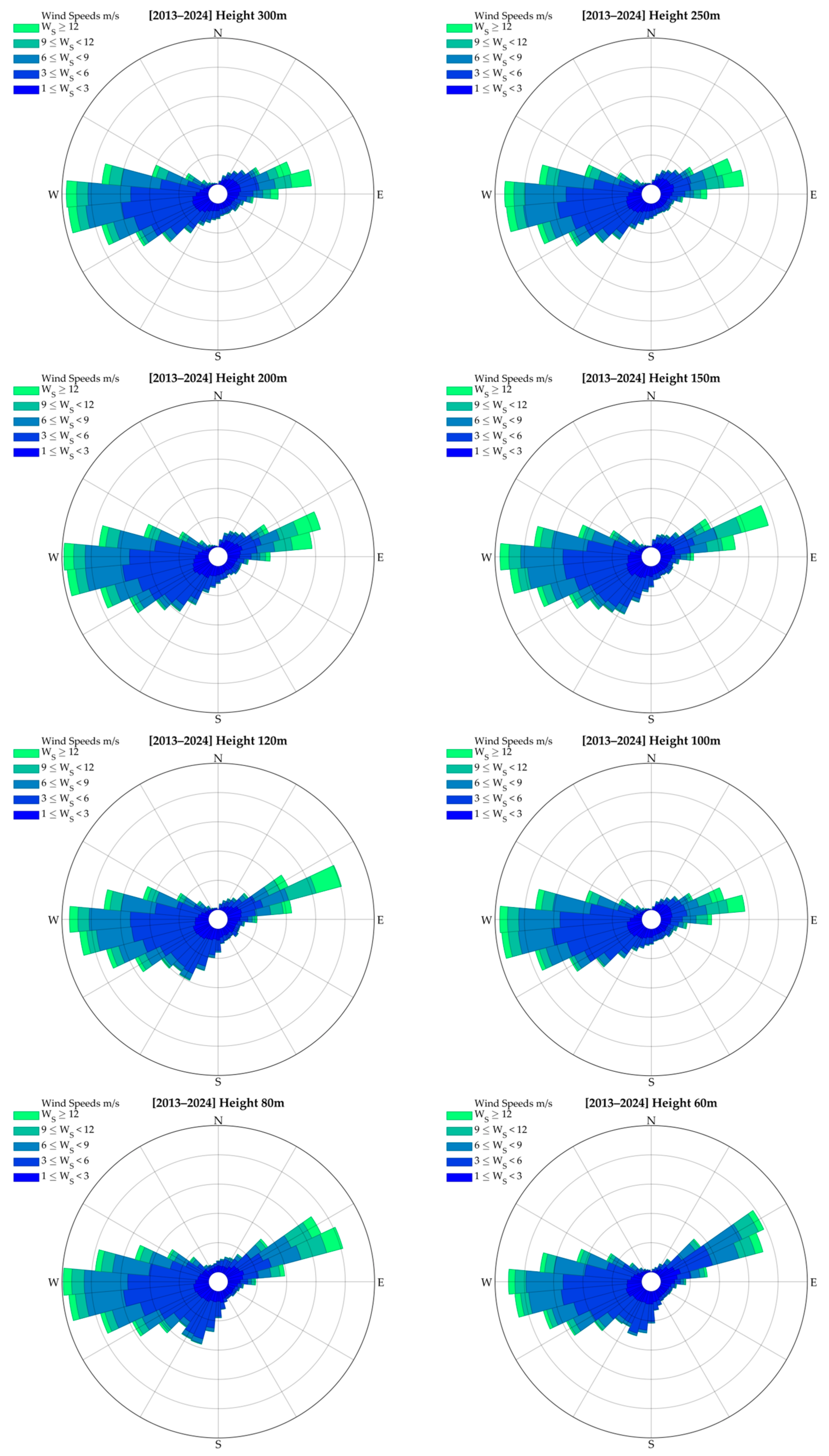
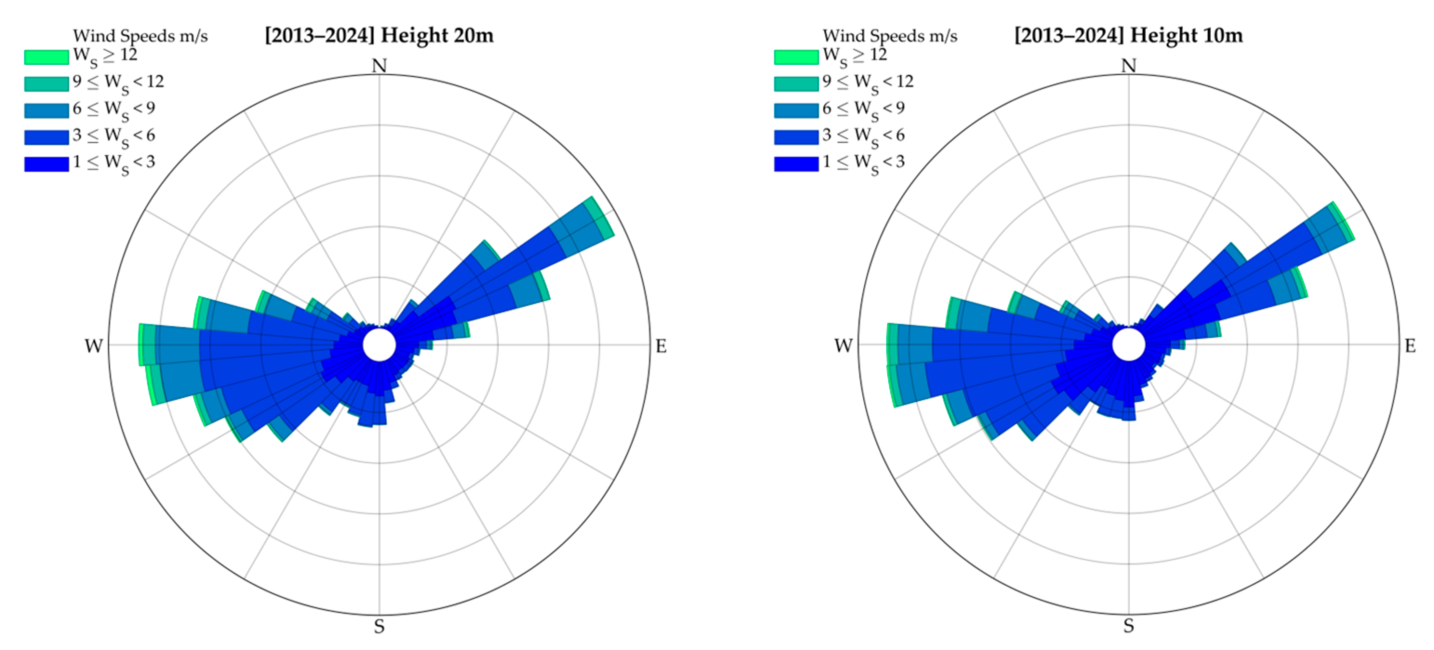
4.1. Wind Rose of WXT520 Data

As shown in Table 1, the two instruments have different coverage rates. Between 2015 and 2023, the combined WXT520 coverage rate was 94.20%, which allowed for the generation of a wind rose showing the main characteristics of near-surface (10 m AGL) circulation at the LMT observation site (Figure 2).

The wind rose clearly shows the presence of two well-defined wind corridors: a western wind corridor and a northeastern corridor. These wind patterns are the result of local orography and its peculiarities.

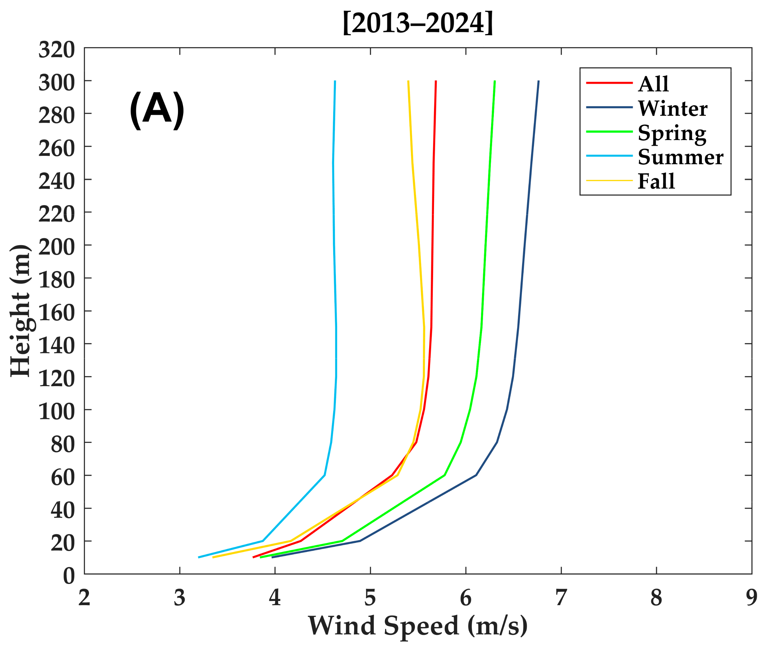
4.2. Vertical Wind Profiles of ZephIR 300 Data

ZephIR 300 operations at LMT are characterized by the presence of various gaps caused by maintenance issues (Table 1). Between 2013 and 2024, several years lack measurements. However, the available data have allowed for the generation of vertical wind profiles based on the ten altitude thresholds mentioned in Section 3 (Figure 3).

From these profiles, it is possible to infer that the western component becomes stronger at higher altitudes, which is in accordance with large-scale flows reported in the literature [35].

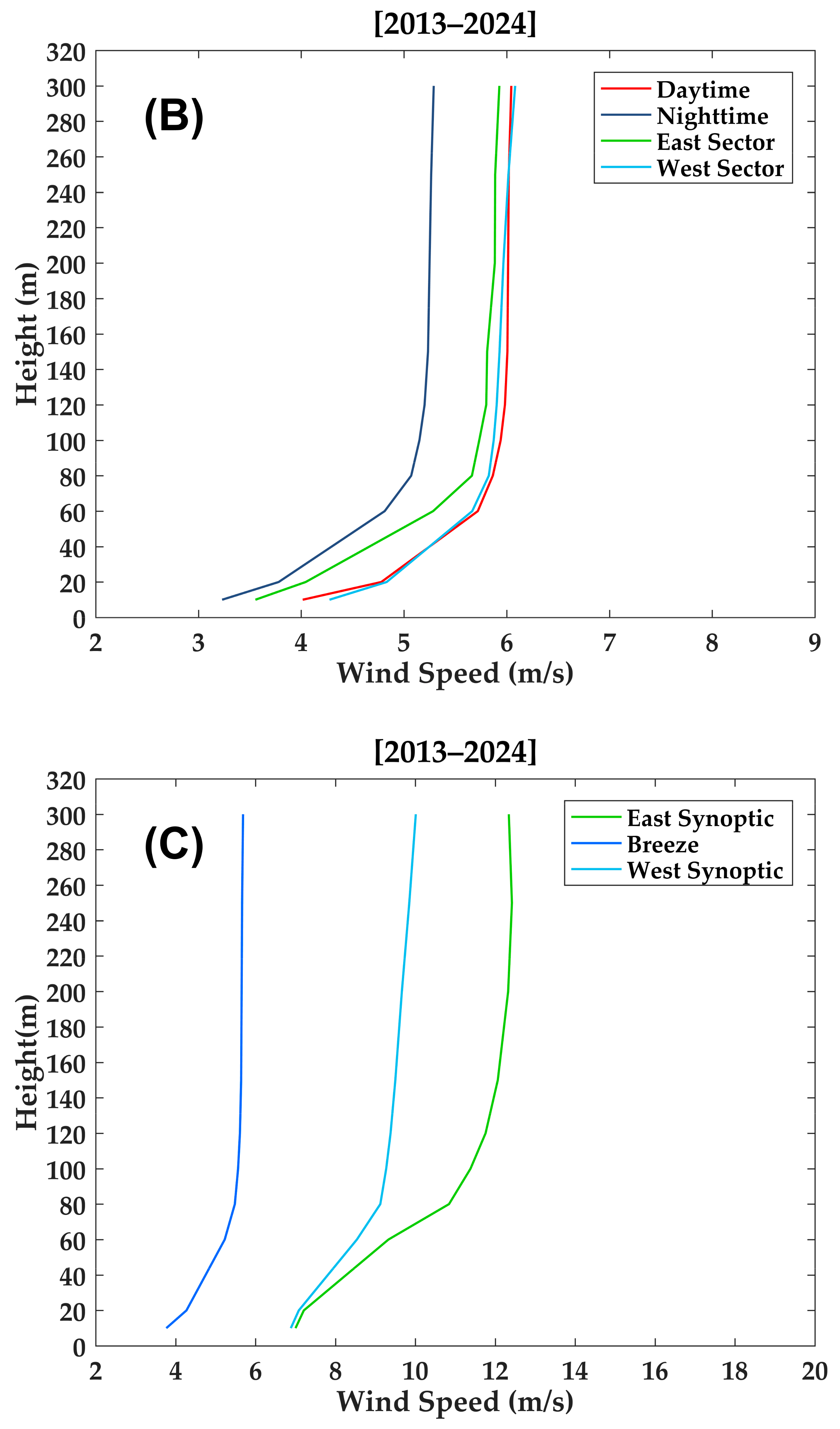
4.3. Wind Profiles Differentiated by Category

In addition to the evaluation of wind profiles based on wind directions and selecting altitude thresholds, additional evaluations targeted seasonal and wind regime variability. The results are shown in Figure 4.

These categories are based on the findings of previous studies, such as those by Cristofanelli et al. (2017) [28] and D’Amico et al. (2024e) [34], showing the complexity of data variability at LMT.

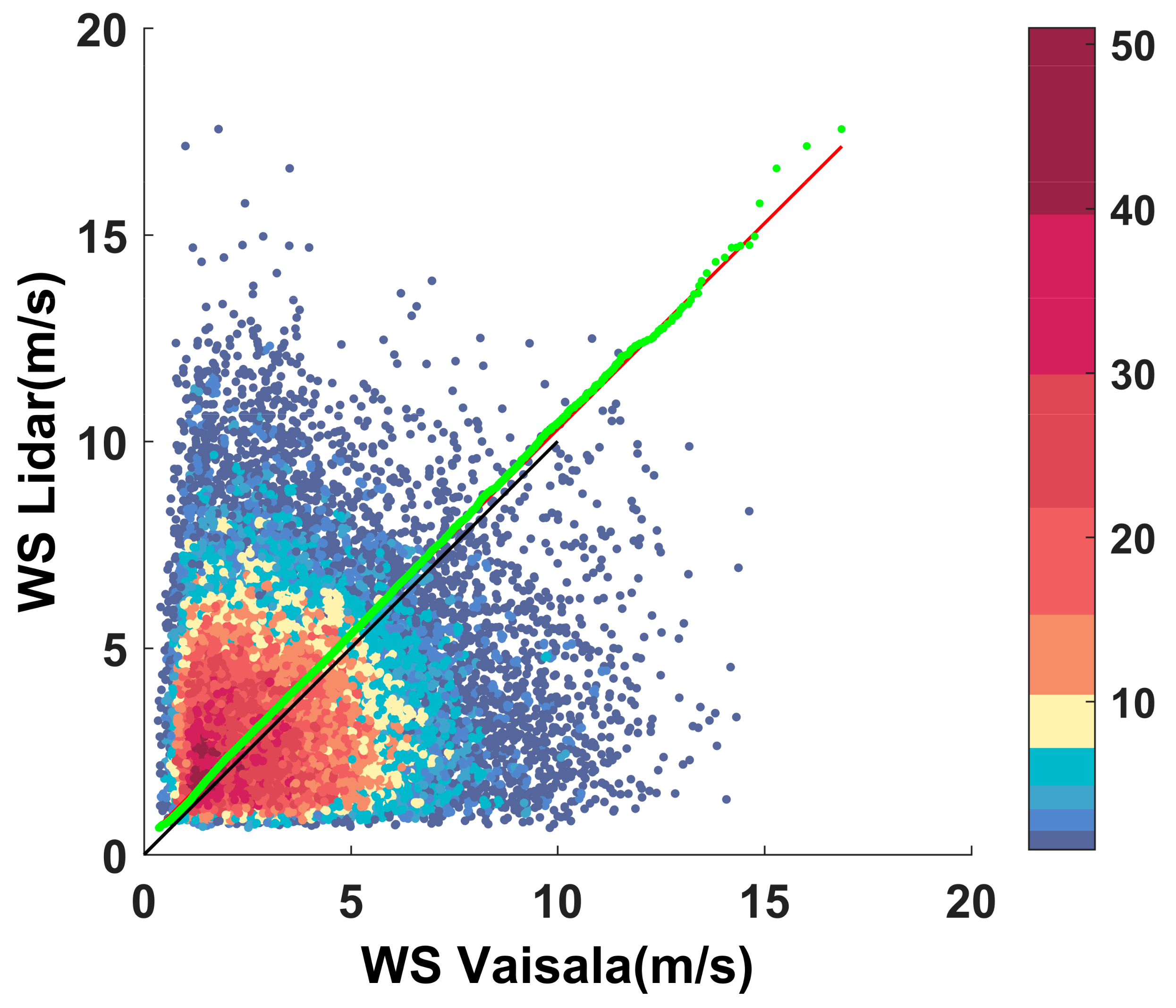
4.4. Comparison Between Near-Surface Vaisala and ZephIR Measurements

Vaisala WXT520 data and the lowermost layer measured by the ZephIR 300 wind lidar were compared to their agreement, i.e., whether wind speeds observed at 10 m AGL by the WXT520 agree with their counterparts measured by lidar. A quantile plot (q-plot), shown in Figure 5, compares these measurements.

Figure 5 shows a higher density for low values of wind speed (<6 m/s), while the density decreases (blue color) for very high values of wind speed, representing extreme events in the record. Overall, the trend is linear. However, some dispersion is present, especially at higher wind speeds.

The comparison between these measurements was further assessed using additional statistical parameters, such as Pearson’s Correlation Coefficient (PCC) [85,86]. The results of this evaluation are shown in

Table 6. Root Square Error (RMSE), bias, Pearson’s Correlation Coefficient (PCC), intercept, and Scatter Index (SI) of the comparison between WXT520 wind speeds at 10 m AGL and ZephIR 300 wind speeds at the same height.

RSE	Bias	PCC	Interc.	SI
2.846	0.264	0.003	3.502	0.826

.

This slightly positive bias (0.264) indicates that—on average—ZephIR measurements are higher than their Vaisala counterparts. The very low correlation (PCC = 0.003) suggests there is almost no linear relationship between the two datasets.

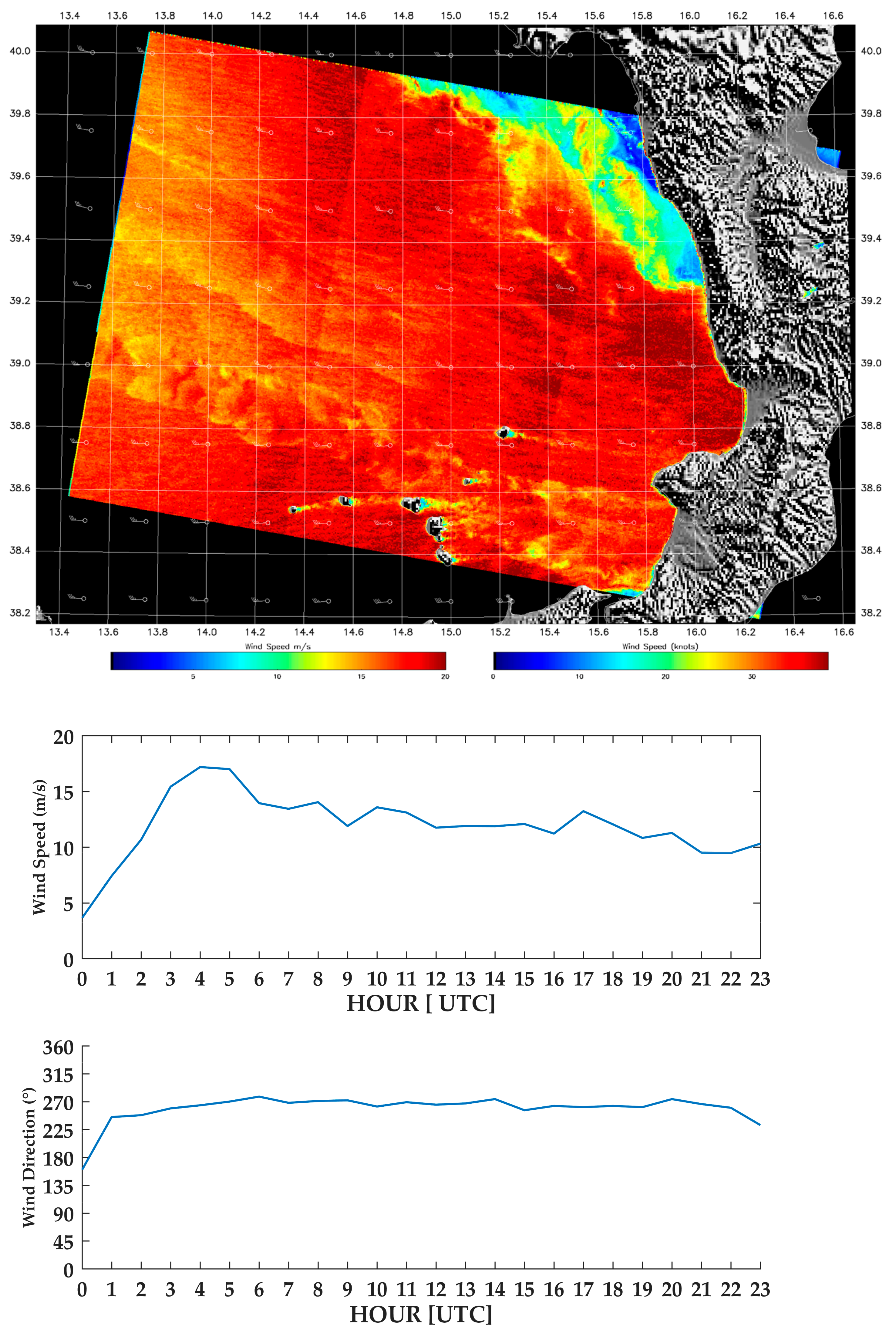
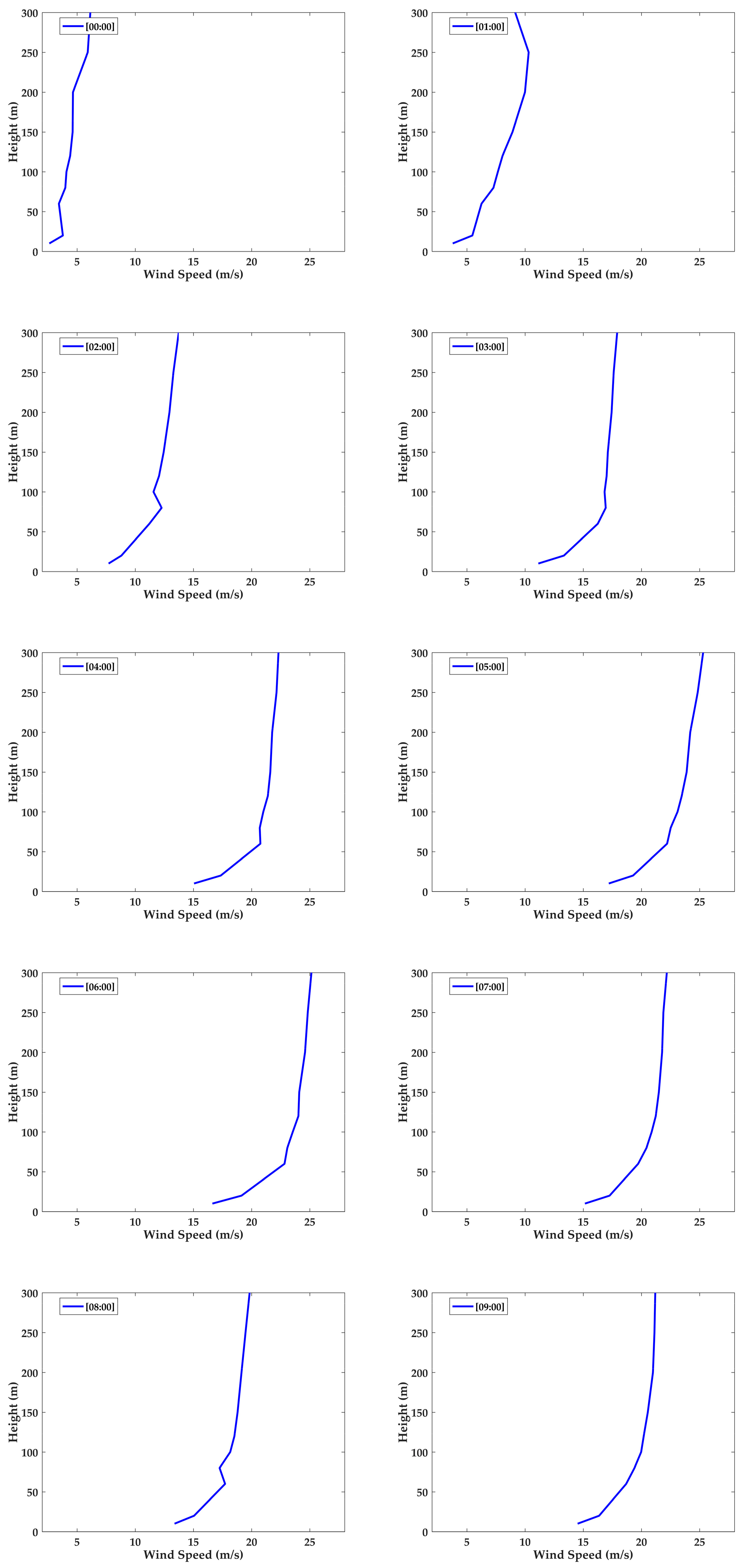
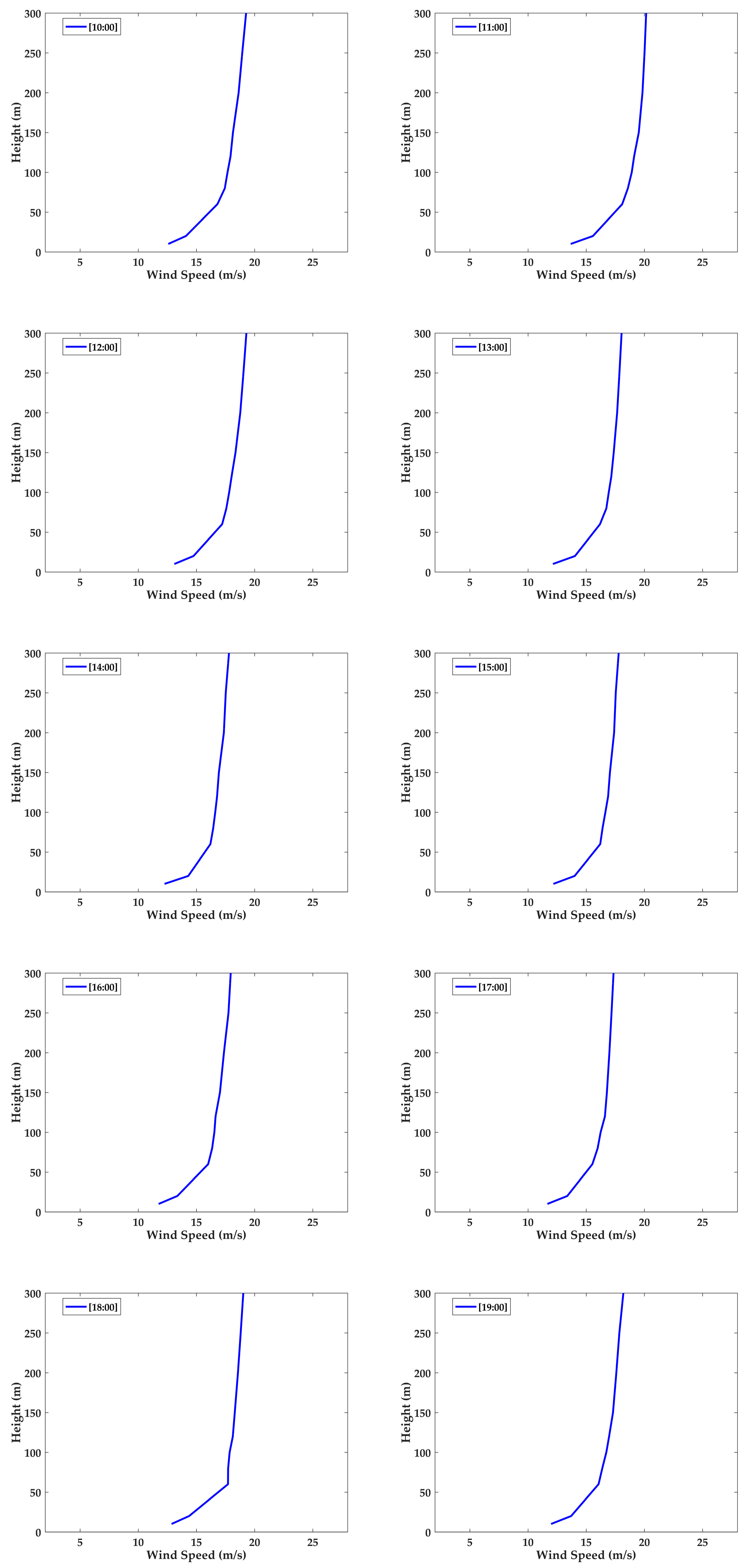
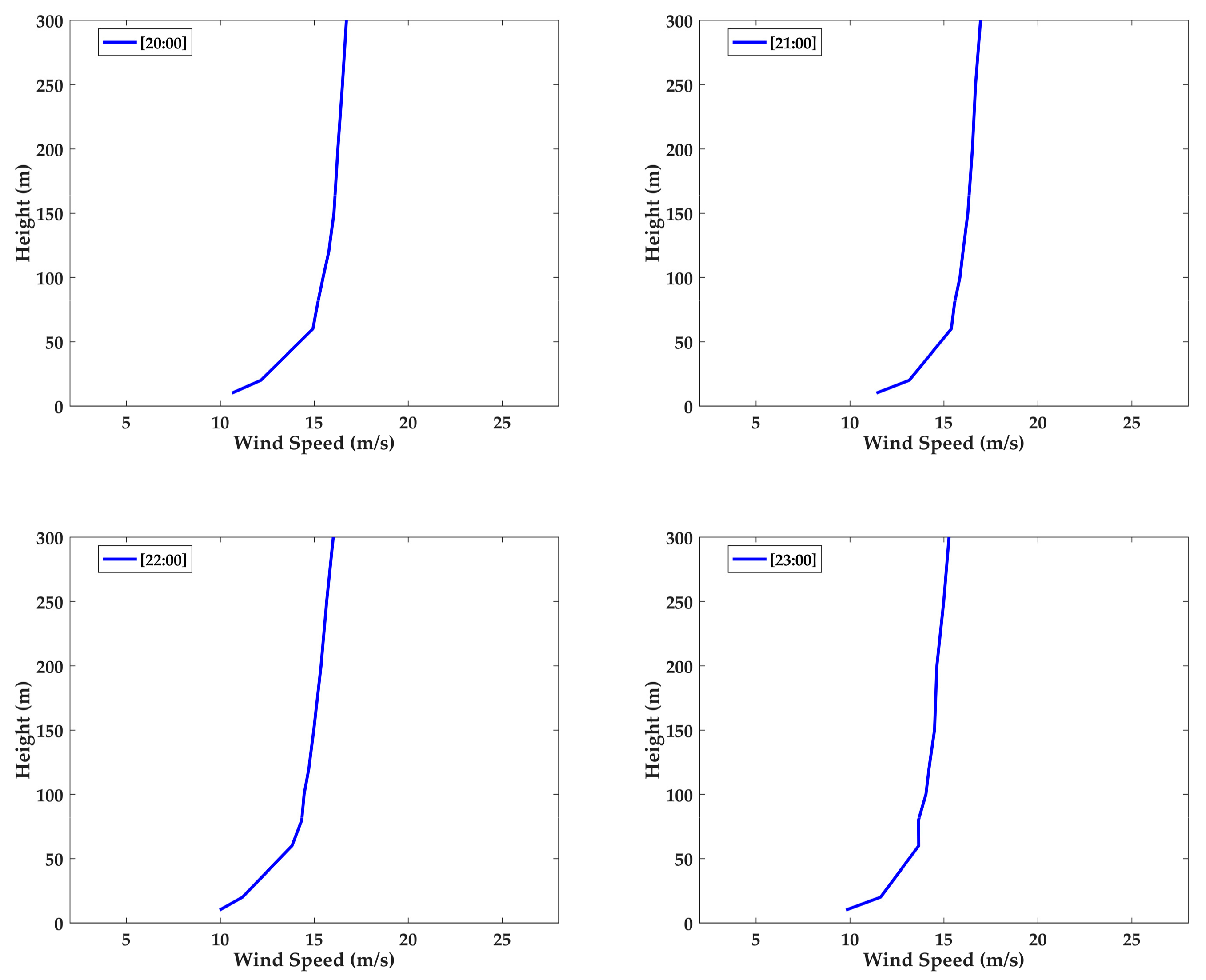
4.5. Case Study: 7 January 2024

In the present work, a case study was selected to show wind patterns and speeds under exceptional conditions. The CS was also selected based on instrument and data availability in order to integrate WXT520 and ZephIR 300 measurements at LMT with SAR imaging of the area and therefore provide a detailed framework for local-to-large scale circulation. In Figure 6, SAR imaging and WXT520 data are shown: the latter, in particular, highlight a persistent westerly wind, without the exception of the early hour.

These conditions were matched by high speeds detected by LMT’s wind lidar, as shown in Figure 7.

These hourly vertical profiles show the evolution of the CS as a time lapse, with wind speeds steadily above the 10 m/s threshold and peaks above 25 m/s.

5. Discussion

5.1. Data Variability Through Select Altitude Thresholds

At the WMO/GAW (World Meteorological Organization—Global Atmosphere Watch) observation site of Lamezia Terme (code: LMT) in Calabria, Southern Italy, a decade of continuous records of surface and near-surface wind data were evaluated to provide a more detailed understanding of local circulation at the site. This evaluation is based on the longest time series analysis ever performed at the LMT site. The station is located in a unique environment in the Italian peninsula, where the distance between the Tyrrhenian and Ionian coasts is ≈32 km (Figure 1). The peculiar geodynamical processes influencing the Calabria–Peloritani Arc (CPA) and extensional faulting have reshaped local geomorphology and set up the Catanzaro isthmus, a former tidal strait [37,39] characterized by wind circulation patterns well oriented on an E-W axis [5,35]. The local complexity of the area where LMT is located adds up to the processes affecting the Mediterranean Basin as a whole. In fact, the Mediterranean itself is considered a hotspot for climate mechanisms and air mass transport [87,88,89,90,91]. Soukissian and Sotiriou (2022) [92] remarked on the importance of the detailed characterization of wind patterns in the Basin as additional tools towards a more accurate understanding of climate mechanisms in the sector.

This study highlights the importance of data coverage in the evaluation of wind patterns. Two key instruments, the Vaisala WXT520 weather station and the ZephIR 300 wind lidar, demonstrate different coverage rates throughout the study period (2013–2024) (Table 1). The WXT520 is characterized by a shorter operating period (2015–2023), while the ZephIR encompasses the entire decade but is heavily affected by maintenance issues, which caused significant reductions in data coverage rates. Despite this, a sufficient amount of data was gathered to adequately assess near-surface wind patterns at LMT.

The main statistics of WXT520 measurements are shown in Table 2. In addition to a differentiation by wind sector, changes over time in average wind speeds are noticeable. In 2015, the mean was 3.15 m/s, while in 2022, it decreased to 3.01 m/s. The highest mean was reported in 2016 (3.76 m/s). Over the years, the wind speeds exhibit fluctuations, with notable reductions in certain years (e.g., 2022 at 3.01 m/s, as reported above), possibly attributed to changes in environmental factors or atmospheric dynamics. With respect to maximum wind speeds, a peak was observed in 2019 (16.9 m/s), which is considerably higher than the maximum values reported in other years (e.g., 2022, at 11.6 m/s). This underscores the variability in wind conditions and the potential for extreme wind events, which diminish with height but remain consistent in overall trends. The standard deviation (SD) in wind speeds for 2019 was 2.08 m/s compared to the relatively lower variability in 2022 at 1.97 m/s. This indicates more stability in wind conditions during recent years. The yearly trends and percentile data suggest a general decline in mean and maximum wind speeds from 2016 through 2022, which could impact energy production considerations at various heights. The analysis reinforces the need to evaluate both mean conditions and extremes when designing wind resource projects, as variability plays a critical role in energy yield reliability. The wind rose shown in Figure 2 allows for the correlation of these statistics with the main wind corridors known from literature [5,34,35].

The main statistics of ZephIR 300 measurements divided by wind sector (Table 3, Table 4 and Table 5) also assess the degrees of variability over time. The differences in mean annual wind speeds between 300 m and 10 m emphasize the impact of height and how it reflects the characteristics of local wind circulation. The wind roses shown in Figure 3, set at the ten distinct altitude thresholds used in this study (300 m, 250 m, 200 m, 150 m, 120 m, 100 m, 80 m, 60 m, 20 m, and 10 m), allow for the determination of the interplay of near-surface wind circulation and large scale flows. Lower heights are heavily affected by the two axis patterns already reported by WXT520 measurements, while high-altitude thresholds show the influence of westerly winds dominating large-scale flows in the area [5,35]. As reported in Table 3, Table 4 and Table 5, wind speeds at 300 m are substantially higher than those at 10 m, showcasing typical atmospheric wind patterns. The gradient of wind speed reduction from 300 m to 10 m follows an exponential-like decrease, with the most significant differences observed at higher altitudes. The year of maximum wind speed, 2018, at 300 m, peaked at 25.4 m/s, while at 10 m, it reached 14.7 m/s, resulting in a net difference of 10.7 m/s between these height thresholds. There is a clear and expected reduction in wind speed with decreasing height, driven by surface-level interactions and friction. The statistical data demonstrate the expected behavior of wind speed variation with height, with notable differences both in annual means and during extreme wind conditions.

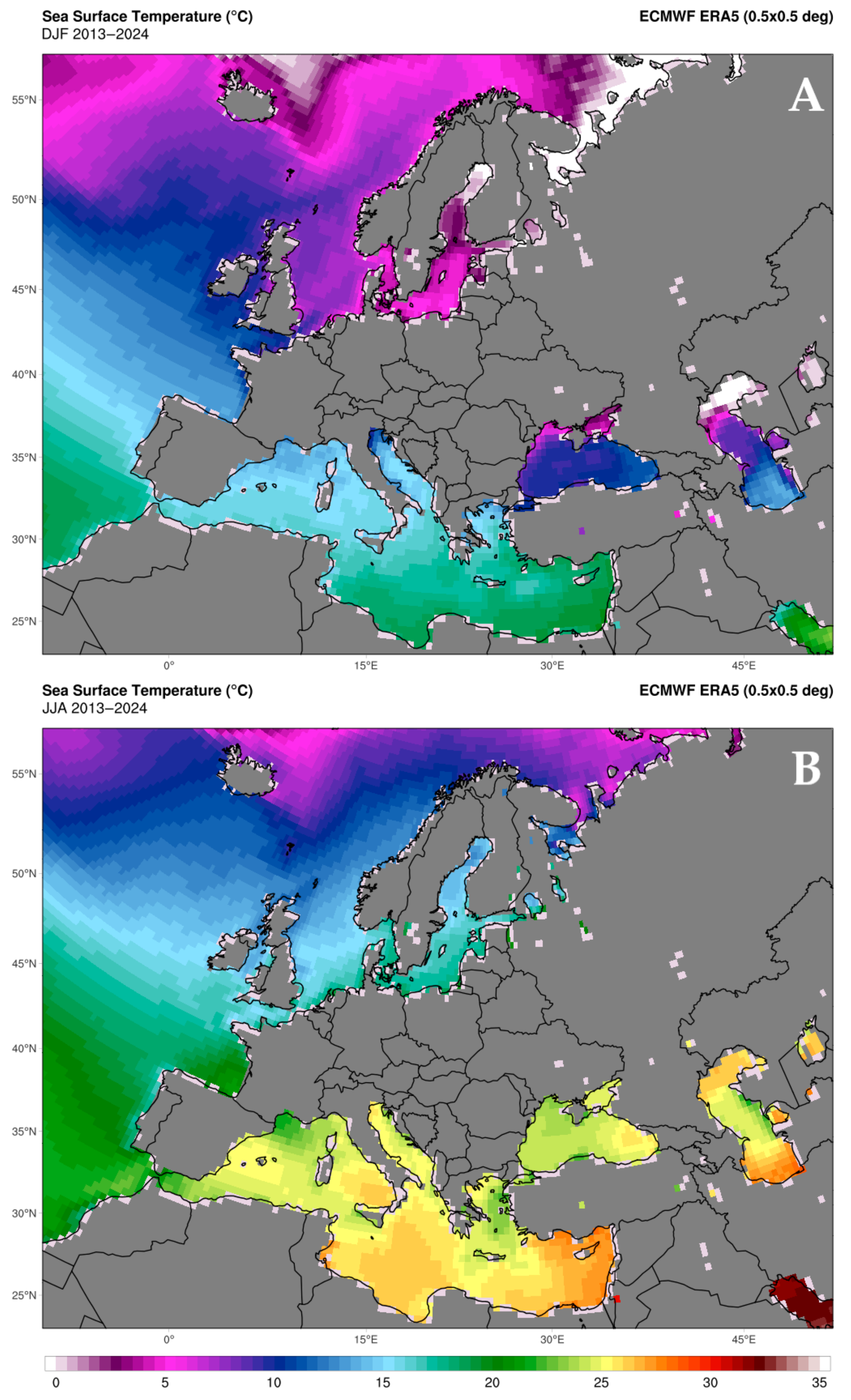
5.2. Seasonal Variability

At the LMT site, differences in environmental parameters are frequently caused by seasonal and day/night cycles [5,35]. In this work, for the first time in the records of the observation site, multi-year data gathered by ZephIR 300 were categorized based on the findings of previous studies, such as those by D’Amico et al. (2024e) [34] (Figure 4). Recent studies on the local wind circulation at the LMT site were limited to surface wind speeds and directions and called for a more detailed characterization of near-surface patterns and their influence on the diffusion and dispersion of gases and aerosols.

Seasonal variability is shown in Figure 4A. During the summer, strong, frequent, and intense diurnal breeze and a weak nocturnal breeze are developed due to the peculiar orographic configuration of the isthmus but also due to the strong difference between land surface temperatures and the SST (Sea Surface Temperature) [93]. In fact, this difference during the daytime reaches its maximum, while the nighttime difference reaches its minimum. During winter and fall, the nocturnal difference between sea and land surface temperatures reaches a maximum value, while the diurnal difference is at its minimum value. This causes frequent nocturnal breezes despite the large-scale forcing that is usually opposed to local-scale flows [5,35].

In Figure 8, ECMWF (European Center Medium Weather Forecast) ERA5 products are shown as highlighting SST monthly averages during the winter (JFD) and summer (JJA) seasons, yielding a difference in the order of 12 °C.

The datasets used for the retrieval of SST maps consist of the ECMWF European Reanalysis V5 (ERA5) [0.25° × 0.25°], downloaded from Copernicus C3S (Climate Change Service). The data files here are re-gridded to 0.5° × 0.5° using bilinear interpolation to reduce server load and access time [94]. The main characteristics of atmospheric flow regimes in the area are that sea breezes have the same direction as western synoptic winds (Figure 4B), as the daytime profile is similar to the western and breeze profiles. Wind regime categorization is shown in Figure 4C. Wind regimes have well-defined differences in wind speeds peaks, as the western synoptics yields speeds greater than 10 m/s. During sunny daytime, sea breeze is always starting and attempts to overimpose on the synoptic winds; conversely, during nighttime hours, the eastern land breeze from is suppressed. During synoptic winds, stability conditions of the atmosphere are near neutral—likely due to the higher wind speed than during sea breeze—whereas during the sea–land breeze regimes, there the typical unstable-stable daily cycles.

5.3. Comparisons Between Employed Instruments and Future Perspectives

Although the two instruments operate under different measurement principles, their data-gathering operations overlap at the 10 m AGL height mark, thus allowing for a direct comparison, which, in this work, is evaluated via a q-plot/scatter plot (Figure 5) and correlation parameters (Table 6). In the plot, data points show a reasonably linear trend, though with some dispersion, especially at higher wind speeds. Color intensity corresponds to data density; the red line indicates a fit to the data (possibly a regression line). The black diagonal line represents the ideal one-to-one relationship, while the green line represents a quantile/quantile (Q-Q) comparison curve, hence the q-plot. The comparison between wind speeds measured at a 10 m height by both instruments reveals certain statistical errors that provide insights into the performance and reliability of the instruments, particularly in a coastal environment. The Root Squared Error (RSE = 2.84 m/s) reflects the average deviation between the two measurements. Specifically, an RSE value of 2.84 m/s is relatively high, suggesting significant variation in the measurements, which is likely caused by turbulence, atmospheric conditions, or differences in sensor response. Coastal environments, characterized by rapidly changing winds, high turbulence, and localized wind effects (e.g., gusts or shears), likely contribute to this error. The bias parameter also reported in Table 6 (0.26 m/s) indicates that, on average, the ZephIR measures wind speeds 0.26 m/s higher than the WXT520. This is a small offset that may result, for instance, from differences in the principles of measurement of both devices, as they indeed operate differently and show a different sensitivity to changes in wind speed. Coastal sites might amplify the bias due to rapid shifts in wind direction and varying gust intensities.

A very low linear correlation coefficient of 0.004 suggests a low linear relationship between the two measurements, but this value could be affected by outliers, as notable deviations at extreme wind speeds could heavily affect the correlation parameter itself. It is also worth mentioning that coastal winds often involve non-linear wind profiles and localized gusts, which could disrupt linear correlations. Furthermore, sensors may respond differently to turbulence or vertical wind components, which are also common in coastal areas. A scatter index (SI) of 0.82 quantifies the variability in the differences relative to the mean wind speed. In this evaluation, the SI is high and reflects large relative deviations. This is also attributable to the characteristics of coastal sites, i.e., turbulent winds, vertical wind shear, and interactions between land and sea breezes. Coastal areas are also characterized by high humidity and the presence of salt particles, which may impact wind lidar performance by perturbing the backscatter signal and degrading its accuracy compared to the WXT520 system. Overall, while the bias is relatively small, high RSE and SI parameters show significant measurement variability at the 10 m AGL height threshold. The low PCC may indicate a prominent influence of the vertical component of near-surface winds.

In order to complement the multi-year analysis, a case study (7 January 2024) was presented based on the coverage of multiple surface instruments and SAR imaging. The SAR product in Figure 6 shows an event that widely influenced the Tyrrhenian coast of Calabria and, due to the particular configuration of the Catanzaro isthmus, resulted in strong westerly winds being channeled through the isthmus itself, exploiting the absence of obstacles. The interaction between strong winds and physical obstacles located west of the observatory, i.e., the Aeolian Islands, can also be noticed. WXT520 measurements at LMT show a consistent westerly pattern throughout the entire day and a surge in wind speeds, up to 17.18 m/s at 04:00 UTC, followed by a progressive decline. Wind profiles by ZephIR 300 (Figure 7) show peaks of 25 m/s at 04:00–05:00 UTC at the highest thresholds, followed by a decline throughout the case study.

Overall, the findings of this study contribute to a more comprehensive understanding of wind circulation in an area characterized by geomorphological peculiarities that are unique in the context of the Italian peninsula. As a growing number of meteorological stations in the country begin advanced measurements of wind parameters [95,96], detailed studies based on such methodologies can set up the fundaments for additional renewable energy exploitation, which itself is one of the key challenges towards sustainable development goals [97,98]. This can also be achieved via the release of datasets covering long time series of data, which can be used to better understand tendencies and possible correlations with climate mechanisms. In addition to the renewable energy sector, these findings are of interest also in the field of air quality control and monitoring: past research on LMT data aimed at greenhouse gases and aerosols—including combustion outputs which are not beneficial for the environment and human health—linked local wind circulation patterns to peaks in a number of parameters [28,30,34,56,99,100,101,102]. Specifically, wind inversion patterns typical of LMT’s local circulation were proven to cause the precipitation and therefore peaks in pollutants that would otherwise be subject to transport at higher altitudes. However, without detailed wind measurements at several altitude thresholds from the surface, these assumptions were founded on surface wind data alone gathered by the Vaisala WXT520 instrument. In this study, the multi-year characterization of wind profiles at the site shows a clear shift in prevailing wind directions as the altitude increases, which is in accordance with pollutant precipitation events reported in previous works [34,102]. Moreso, as the interplay of gases, aerosols, and wind pattern regulates the concentrations of key parameters, methodologies aimed at the evaluation of atmospheric background levels also need to consider the wind data variability evidenced in this study to better discriminate air masses subject to recent anthropic activity from those representative of the northern hemisphere’s atmospheric background [103].

6. Conclusions

A decade (2013–2024) of measurements performed by Vaisala WXT520 weather station and a ZephIR 300 wind lidar were evaluated to provide a more accurate understanding, compared to previous studies, of surface and near-surface wind circulation patterns at the southern Italian WMO/GAW observation site of Lamezia Terme (LMT) in Calabria. Data coverage is affected by maintenance issues associated with the ZephIR lidar. However, a multi-year evaluation accounting for several parameters (seasons, day/night cycles, and wind regimes) enabled the better characterization of wind patterns in the area. This work constitutes the longest evaluation of a time series to date at the LMT site.

The Lamezia Terme station captures the complexity of Mediterranean coastal meteorology; the near-neutral conditions during synoptic winds and the unstable/stable cycle of the sea–land breeze regimes highlight the interaction of large-scale and local factors. These processes are amplified during summer by strong thermal contrasts between land and sea, further modulated by the region’s orographic setting. In the study area, both synoptic and sea breeze regimes are westerly advecting marine aerosols inland. The sea breeze always develops, modulating the synoptic flow, while the land breeze is overdriven by the synoptic flow that blows from the opposite direction.

During synoptic westerly winds, the atmosphere exhibits near-neutral stability conditions: this is attributed to the higher wind speeds overriding the effects of surface heating and cooling. The influence of the Tyrrhenian Sea moderates the surface fluxes, maintaining a relatively steady state. In this study, it is reported that wind directions under breeze regimes changed past the 100 m AGL altitude threshold in accordance with large-scale flows influencing the area. As near-surface winds are oriented on an E-W axis, which matches the configuration of the isthmus where the site is located, large-scale flows tend to dominate at higher altitudes. During night hours, the land breeze is light, often contrasted by the synoptic westerly flow.

In this study, data from the two instruments gathered at the same height threshold of 10 m AGL were statistically evaluated, showing the presence of biases and scatters in the distribution, which likely depend on a combination of technical and environmental factors. Furthermore, a single case study linked to strong westerly speeds was described by integrating surface measurements with SAR imaging over a regional scale.

These findings are essential for improving the accuracy of atmospheric models, renewable energy resource assessments, and pollution transport predictions in coastal regions. By providing high-resolution insights into wind circulation, this work contributes to a better understanding of near-surface processes in coastal environments and their implications for regional meteorology and environmental management. Specifically, the findings have allowed for the demonstration of a number of hypotheses on local mechanisms driving peaks in the concentrations of aerosols and gases, which in turn show the importance of detailed wind pattern characterization in air quality control, especially in areas such as the Italian coastlines which are subject to a combination of natural and anthropic influences.

References

1. Cormier, R. The behavior of vertically integrated boundary-layer winds. Bound.-Lay. Meteorol. 1975, 9, 315–324. [Google Scholar] [CrossRef]
2. Delage, Y. The position of the lowest levels in the boundary layer of atmospheric circulation models. Atmos.-Ocean 1988, 26, 329–340. [Google Scholar] [CrossRef]
3. Rigby, M.; Toumi, R. London air pollution climatology: Indirect evidence for urban boundary layer height and wind speed enhancement. Atmos. Environ. 2008, 42, 4932–4947. [Google Scholar] [CrossRef]
4. Fitch, A.C.; Lundquist, J.K.; Olson, J.B. Mesoscale influences of wind farms throughout a diurnal cycle. Mon. Weather Rev. 2013, 141, 2173–2198. [Google Scholar] [CrossRef]
5. Federico, S.; Pasqualoni, L.; Sempreviva, A.M.; De Leo, L.; Avolio, E.; Calidonna, C.R.; Bellecci, C. The seasonal characteristics of the breeze circulation at a coastal Mediterranean site in South Italy. Adv. Sci. Res. 2010, 4, 47–56. [Google Scholar] [CrossRef]
6. Sørensen, S.T.; Warden, M.; Macarthur, J.; Silver, M.; Holtom, T.C.; McDonald, C.; Clive, P.; Bookey, H.T. Advances in Doppler Lidar for accurate 3D wind measurements. In Imaging and Applied Optics; Optica Publishing Group: Orlando, FL, USA, 2018; p. AM2A.3. [Google Scholar] [CrossRef]
7. Hieronimus, J. Wind Speed Measurements in an Offshore Wind Farm by Remote Sensing: A Comparison of Radar Satellite TerraSAR-X and Ground-Based LiDAR Systems; University of Oldenburg: Oldenburg, Germany, 2015. [Google Scholar]
8. Gullì, D.; Avolio, E.; Calidonna, C.R.; Lo Feudo, T.; Torcasio, R.C.; Sempreviva, A.M. Two years of wind-lidar measurements at an Italian Mediterranean Coastal Site. Energy Procedia 2017, 125, 214–220. [Google Scholar] [CrossRef]
9. Li, N.; Dyer-Hawes, Q.; Romanic, D.; Burlando, M. Investigation of coastal winds and turbulence characteristics using Doppler lidar. J. Geophys. Res. Atmos. 2024, 129, e2024JD041429. [Google Scholar] [CrossRef]
10. Suo, C.; Sun, A.; Yan, C.; Cao, X.; Peng, K.; Tan, Y.; Yang, S.; Wei, Y.; Wang, G. Quality Assessment of ERA5 Wind Speed and Its Impact on Atmosphere Environment Using Radar Profiles along the Bohai Bay Coastline. Atmosphere 2024, 15, 1153. [Google Scholar] [CrossRef]
11. Menezes, I.C.; Lopes, D.; Fernandes, A.P.; Borrego, C.; Viegas, D.X.; Miranda, A.I. Atmospheric dynamics and fire-induced phenomena: Insights from a comprehensive analysis of the Sertã wildfire event. Atmos. Res. 2024, 310, 107649. [Google Scholar] [CrossRef]
12. Novitskii, M.A.; Gaitandzhiev, D.E.; Mazurin, N.F.; Matskevich, M.K. Turbulence characteristics in the coastal zone with breeze circulation. Russ. Meteorol. Hydrol. 2011, 36, 580–589. [Google Scholar] [CrossRef]
13. Liu, J.; Song, X.; Long, W.; Fu, Y.; Yun, L.; Zhang, M. Structure analysis of the sea breeze based on Doppler Lidar and its impact on pollutants. Remote Sens. 2022, 14, 324. [Google Scholar] [CrossRef]
14. Puygrenier, V.; Lohou, F.; Campistron, B.; Saïd, F.; Pigeon, G.; Bénech, B.; Serça, D. Investigation on the fine structure of sea-breeze during ESCOMPTE experiment. Atmos. Res. 2005, 74, 329–353. [Google Scholar] [CrossRef]
15. Song, X.; Zhou, T.; Wang, Y.; Li, X.; Wu, D.; Gu, Y.; Lin, Z.; Abdullaev, S.F.; Amonov, M.O. Spatiotemporal evolution of dust over Tarim Basin under continuous clear-sky. Atmos. Res. 2024, 312, 107764. [Google Scholar] [CrossRef]
16. Shu, H.; Zhang, F.; Du, Y.; Wang, Y.; Guo, H.; Song, Z.; Zhang, Q. Characteristics and Formation Mechanisms of Low-Level Jets in Northeastern China. Adv. Atmos. Sci. 2024, 41, 2432–2445. [Google Scholar] [CrossRef]
17. Wei, L.; Zhao, L.; Li, Z.; Li, Y.; Wen, Q.; Ma, Y. Numerical simulation of circulation characteristics of orographic precipitation in Qilian Mountains, Northeastern Tibetan Plateau. Atmos. Res. 2024, 312, 107762. [Google Scholar] [CrossRef]
18. Madonna, F.; De Rosa, B.; Gagliardi, S.; Gandolfi, I.; Essa, Y.H.; Madonna, D.; Marra, F.; Menniti, M.A.; Summa, D.; Tramutola, E.; et al. Water vapour fluxes at a Mediterranean coastal site during the summer of 2021: Observations, comparison with atmospheric reanalysis, and implications for extreme events. Earth Syst. Dyn. Discuss. 2024, 1–21, under review. [Google Scholar] [CrossRef]
19. Davolio, S.; Della Fera, S.; Laviola, S.; Miglietta, M.M.; Levizzani, V. Heavy precipitation over Italy from the Mediterranean storm “Vaia” in October 2018: Assessing the role of an atmospheric river. Mon. Weather Rev. 2020, 148, 3571–3588. [Google Scholar] [CrossRef]
20. Martinez, J.A.; Junquas, C.; Bozkurt, D.; Viale, M.; Fita, L.; Trachte, K.; Campozano, L.; Arias, P.A.; Boisier, J.P.; Condom, T.; et al. Recent progress in atmospheric modeling over the Andes–Part I: Review of atmospheric processes. Front. Earth Sci. 2024, 12, 1427783. [Google Scholar] [CrossRef]
21. Hagay, O.; Brenner, S. Sensitivity of Simulations of Extreme Mediterranean Storms to the Specification of Sea Surface Temperature: Comparison of Cases of a Tropical-Like Cyclone and Explosive Cyclogenesis. Atmosphere 2021, 12, 921. [Google Scholar] [CrossRef]
22. Chronis, T.; Case, J.L.; Papadopoulos, A.; Anagnostou, E.N.; Mecikalski, J.R.; Haines, S.L. Towards improved forecasts of atmospheric and oceanic circulations over the complex terrain of the Eastern Mediterranean. In Proceedings of the American Meteorological Society 88th Annual Meeting, New Orleans, LA, USA, 20–24 January 2008; p. 0013545. Available online: https://ntrs.nasa.gov/citations/20080013545 (accessed on 15 January 2025).
23. Herbaut, C.; Martel, F.; Crépon, M. A sensitivity study of the general circulation of the Western Mediterranean Sea. Part II: The response to atmospheric forcing. J. Phys. Oceanogr. 1997, 27, 2126–2145. [Google Scholar] [CrossRef]
24. Meroni, A.N.; Giurato, M.; Ragone, F.; Pasquero, C. Observational evidence of the preferential occurrence of wind convergence over sea surface temperature fronts in the Mediterranean. Q. J. R. Meteorol. Soc. 2020, 146, 1443–1458. [Google Scholar] [CrossRef]
25. Stathopoulos, C.; Patlakas, P.; Tsalis, C.; Kallos, G. The role of sea surface temperature forcing in the life-cycle of Mediterranean cyclones. Remote Sens. 2020, 12, 825. [Google Scholar] [CrossRef]
26. Ehmele, F.; Barthlott, C.; Corsmeier, U. The influence of Sardinia on Corsican rainfall in the western Mediterranean Sea: A numerical sensitivity study. Atmos. Res. 2015, 153, 451–464. [Google Scholar] [CrossRef]
27. Zhou, X.; Yang, K.; Beljaars, A.; Li, H.; Lin, C.; Huang, B.; Wang, Y. Dynamical impact of parameterized turbulent orographic form drag on the simulation of winter precipitation over the western Tibetan Plateau. Clim. Dyn. 2019, 53, 707–720. [Google Scholar] [CrossRef]
28. Cristofanelli, P.; Busetto, M.; Calzolari, F.; Ammoscato, I.; Gullì, D.; Dinoi, A.; Calidonna, C.R.; Contini, D.; Sferlazzo, D.; Di Iorio, T.; et al. Investigation of reactive gases and methane variability in the coastal boundary layer of the central Mediterranean basin. Elem. Sci. Anth. 2017, 5, 12. [Google Scholar] [CrossRef]
29. D’Amico, F.; Ammoscato, I.; Gullì, D.; Avolio, E.; Lo Feudo, T.; De Pino, M.; Cristofanelli, P.; Malacaria, L.; Parise, D.; Sinopoli, S.; et al. Anthropic-induced variability of greenhouse gases and aerosols at the WMO/GAW coastal site of Lamezia Terme (Calabria, Southern Italy): Towards a new method to assess the weekly distribution of gathered data. Sustainability 2024, 16, 8175. [Google Scholar] [CrossRef]
30. D’Amico, F.; Gullì, D.; Lo Feudo, T.; Ammoscato, I.; Avolio, E.; De Pino, M.; Cristofanelli, P.; Busetto, M.; Malacaria, L.; Parise, D.; et al. Cyclic and multi-year characterization of surface ozone at the WMO/GAW coastal station of Lamezia Terme (Calabria, Southern Italy): Implications for local environment, cultural heritage, and human health. Environments 2024, 11, 227. [Google Scholar] [CrossRef]
31. D’Amico, F.; Lo Feudo, T.; Gullì, D.; Ammoscato, I.; De Pino, M.; Malacaria, L.; Sinopoli, S.; De Benedetto, G.; Calidonna, C.R. Investigation of carbon monoxide, carbon dioxide, and methane source variability at the WMO/GAW station of Lamezia Terme (Calabria, Southern Italy) using the ratio of ozone to nitrogen oxides as a proximity indicator. Atmosphere 2025, 16, 251. [Google Scholar] [CrossRef]
32. Avolio, E.; Federico, S.; Miglietta, M.M.; Lo Feudo, T.; Calidonna, C.R.; Sempreviva, A.M. Sensitivity analysis of WRF model PBL schemes in simulating boundary-layer variables in southern Italy: An experimental campaign. Atmos. Res. 2017, 192, 58–71. [Google Scholar] [CrossRef]
33. Lo Feudo, T.; Calidonna, C.R.; Avolio, E.; Sempreviva, A.M. Study of the Vertical Structure of the Coastal Boundary Layer Integrating Surface Measurements and Ground-Based Remote Sensing. Sensors 2020, 20, 6516. [Google Scholar] [CrossRef]
34. D’Amico, F.; Calidonna, C.R.; Ammoscato, I.; Gullì, D.; Malacaria, L.; Sinopoli, S.; De Benedetto, G.; Lo Feudo, T. Peplospheric influences on local greenhouse gas and aerosol variability at the Lamezia Terme WMO/GAW regional station in Calabria, Southern Italy: A multiparameter investigation. Sustainability 2024, 16, 10175. [Google Scholar] [CrossRef]
35. Federico, S.; Pasqualoni, L.; De Leo, L.; Bellecci, C. A study of the breeze circulation during summer and fall 2008 in Calabria, Italy. Atmos. Res. 2010, 97, 1–13. [Google Scholar] [CrossRef]
36. European Commission. European Marine Observation and Data Network (EMODnet). Available online: https://emodnet.ec.europa.eu/en/bathymetry (accessed on 15 January 2025).
37. Longhitano, S.G. The record of tidal cycles in mixed silici–bioclastic deposits: Examples from small Plio–Pleistocene peripheral basins of the microtidal Central Mediterranean Sea. Sedimentology 2010, 58, 691–719. [Google Scholar] [CrossRef]
38. Chiarella, D.; Longhitano, S.G.; Muto, F. Sedimentary features of the lower Pleistocene mixed siliciclastic-bioclastic tidal deposits of the Catanzaro Strait (Calabrian Arc, south Italy). Rend. Online Della Soc. Geol. Ital. 2012, 21, 919–920. [Google Scholar]
39. Longhitano, S.G.; Chiarella, D.; Muto, F. Three-dimensional to two-dimensional cross-strata transition in the lower Pleistocene Catanzaro tidal strait transgressive succession (southern Italy). Sedimentology 2014, 61, 2136–2171. [Google Scholar] [CrossRef]
40. Brogan, G.E.; Cluff, L.S.; Taylor, C.L. Seismicity and uplift of southern Italy. Tectonophysics 1975, 29, 323–330. [Google Scholar] [CrossRef]
41. Miyauchi, T.; Dai Pra, G.; Sylos Labini, S. Geochronology of Pleistocene marine terraces and regional tectonics in Tyrrhenian coast of South Calabria, Italy. Il Quaternario 1994, 7, 17–34. [Google Scholar]
42. Monaco, C.; Bianca, M.; Catalano, S.; De Guidi, G.; Gresta, S.; Langher, H.; Tortorici, L. The geological map of the urban area of Catania (Sicily): Morphotectonic and seismotectonic implications. Mem. Soc. Geol. Ital. 2001, 5, 425–438. [Google Scholar]
43. Lambeck, K.; Antonioli, F.; Purcell, A.; Silenzi, S. Sea-level change along the Italian coast for the past 10,000 yr. Quat. Sci. Rev. 2004, 23, 1567–1598. [Google Scholar] [CrossRef]
44. Pirazzoli, P.A.; Mastronuzzi, G.; Saliège, J.F.; Sansò, P. Late Holocene emergence in Calabria, Italy. Mar. Geol. 1997, 141, 61–70. [Google Scholar] [CrossRef]
45. Amodio-Morelli, L.; Bonardi, G.; Colonna, V.; Dietrich, D.; Giunta, G.; Ippolito, F.; Liguori, V.; Lorenzoni, P.; Paglionico, A.; Perrone, V.; et al. L’Arco Calabro-Peloritano nell’orogene Appenninico-Maghrebide. Mem. Soc. Geol. Ital. 1976, 17, 1–60. [Google Scholar]
46. Bonardi, G.; De Capoa, P.; Fioretti, B.; Perrone, V. Some remarks on the Calabria-Peloritani arc and its relationship with the southern Apennines. Boll. Geofis. Teor. Appl. 1994, 36, 483–490. [Google Scholar]
47. Scandone, P. Structure and evolution of the Calabrian Arc. Earth Evol. Sci. 1982, 3, 172–180. [Google Scholar]
48. Alvarez, W. A former continuation of the Alps. Geol. Soc. Am. Bull. 1976, 87, 891–896. [Google Scholar] [CrossRef]
49. Malinverno, A.; Ryan, W.B.F. Extension in the Tyrrhenian Sea and shortening in the Apennines as result of arc migration driven by sinking of the lithosphere. Tectonics 1986, 5, 227–245. [Google Scholar] [CrossRef]
50. Critelli, S.; Muto, F.; Tripodi, V.; Perri, F. Relationships between Lithospheric Flexure, Thrust Tectonics and Stratigraphic Sequences in Foreland Setting: The Southern Apennines Foreland Basin System, Italy. In Tectonics 2; Schattner, U., Ed.; Intech Open Access Publisher: Rijeka, Croatia, 2011; pp. 121–170. [Google Scholar] [CrossRef]
51. Nicolosi, I.; Speranza, F.; Chiappini, M. Ultrafast oceanic spreading of the Marsili Basin, southern Tyrrhenian Sea: Evidence from magnetic anomaly analysis. Geology 2006, 34, 717–720. [Google Scholar] [CrossRef]
52. Rosenbaum, G.; Gasparon, M.; Lucente, F.P.; Peccerillo, A.; Miller, M.S. Kinematics of slab tear faults during subduction segmentation and implications for Italian magmatism. Tectonics 2008, 27, 110–116. [Google Scholar] [CrossRef]
53. Cocchi, L.; Caratori Tontini, F.; Muccini, F.; Marani, M.P.; Bortoluzzi, G.; Carmisciano, C. Chronology of the transition from a spreading ridge to an accretional seamount in the Marsili backarc basin (Tyrrhenian Sea). Terra Nova 2009, 21, 369–374. [Google Scholar] [CrossRef]
54. Ventura, G.; Milano, G.; Passaro, S.; Sprovieri, M. The Marsili Ridge (Southern Tyrrhenian Sea, Italy): An island-arc volcanic complex emplaced on a ‘relict’ back-arc basin. Earth Sci. Rev. 2013, 116, 85–94. [Google Scholar] [CrossRef]
55. Palmiotto, C.; Braga, R.; Corda, L.; Di Bella, L.; Ferrante, V.; Loreto, M.F.; Muccini, F. New insights on the fossil arc of the Tyrrhenian Back-Arc Basin (Mediterranean Sea). Tectonophysics 2022, 845, 229640. [Google Scholar] [CrossRef]
56. D’Amico, F.; Lo Feudo, T.; Gullì, D.; Ammoscato, I.; De Pino, M.; Malacaria, L.; Sinopoli, S.; De Benedetto, G.; Calidonna, C.R. Integrated Surface and Tropospheric Column Analysis of Sulfur Dioxide Variability at the Lamezia Terme WMO/GAW Regional Station in Calabria, Southern Italy. Environments 2025, 12, 27. [Google Scholar] [CrossRef]
57. van Dijk, J.P.; Scheepers, P.J.J. Neotectonic rotations in the Calabrian Arc; implications for a Pliocene-Recent geodynamic scenario for the Central Mediterranean. Earth Sci. Rev. 1995, 39, 207–246. [Google Scholar] [CrossRef]
58. Martini, I.P.; Sagri, M.; Colella, A. Neogene—Quaternary basins of the inner Apennines and Calabrian arc. In Anatomy of an Orogen. The Apennines and Adjacent Mediterranean Basins; Vai, G.B., Martini, I.P., Eds.; Kluwer Academic Publishers: Dordrecht, The Netherlands, 2001; pp. 375–400. [Google Scholar] [CrossRef]
59. Cifelli, F.; Mattei, M.; Rossetti, F. Tectonic evolution of arcuate mountain belts on top of a retreating subduction slab: The example of the Calabrian Arc. J. Geophys. Res. Solid Earth 2007, 112, 101. [Google Scholar] [CrossRef]
60. Galli, P.; Bosi, V. Paleoseismology along the Cittanova fault: Implications for seismotectonics and earthquake recurrence in Calabria (southern Italy). J. Geophys. Res. Solid Earth 2002, 107, 2044. [Google Scholar] [CrossRef]
61. Tansi, C.; Folino Gallo, M.; Muto, F.; Perrotta, P.; Russo, L.; Critelli, S. Seismotectonics and landslides of the Crati Graben (Calabrian Arc, Southern Italy). J. Maps 2016, 12 (Suppl. S1), 363–372. [Google Scholar] [CrossRef]
62. Monaco, C.; Tortorici, L. Active faulting in the Calabrian arc and eastern Sicily. J. Geodyn. 2000, 29, 407–424. [Google Scholar] [CrossRef]
63. Ghisetti, F. Evoluzione neotettonica dei principali sistemi di faglie della Calabria centrale. Boll. Soc. Geol. Ital. 1979, 98, 387–430. [Google Scholar]
64. Langone, A.; Gueguen, E.; Prosser, G.; Caggianelli, A.; Rottura, A. The Curinga-Girifalco fault zone (northern Serre, Calabria) and its significance within the Alpine tectonic evolution of the western Mediterranean. J. Geodyn. 2006, 42, 140–158. [Google Scholar] [CrossRef]
65. Rovida, A.; Locati, M.; Camassi, R.; Lolli, B.; Gasperini, P. The Italian earthquake catalogue CPTI15. Bull. Earthq. Eng. 2020, 18, 2953–2984. [Google Scholar] [CrossRef]
66. Rovida, A.; Locati, M.; Camassi, R.; Lolli, B.; Gasperini, P.; Antonucci, A. Catalogo Parametrico dei Terremoti Italiani (CPTI15), versione 4.0. Istituto Nazionale di Geofisica e Vulcanologia (INGV). Available online: https://emidius.mi.ingv.it/CPTI15-DBMI15_v3.0/ (accessed on 20 January 2025).
67. Marino, C.; Misiani, P.; Nucara, A.; Pietrafesa, M. The effect of the climatic condition on the radiant asymmetry. Int. J. Heat Technol. 2017, 35, S419–S426. [Google Scholar] [CrossRef]
68. Wouters, D.A.J.; Wagenaar, J.W. Verification of the ZephIR 300 LiDAR at the ECN LiDAR Calibration Facility for the Offshore Europlatform Measurement Campaign, ECN-M-16-029. Available online: https://resolver.tno.nl/uuid:0e900067-df59-4c76-8f4a-469754ab4d3d (accessed on 20 January 2025).
69. Calidonna, C.R.; Gullì, D.; Avolio, E.; Federico, S.; Lo Feudo, T.; Sempreviva, A. One year of vertical wind profiles measurements at a Mediterranean coastal site of South Italy. Energy Procedia 2015, 76, 121–127. [Google Scholar] [CrossRef]
70. Knoop, S.; Bosveld, F.C.; de Haij, M.J.; Apituley, A. A 2-year intercomparison of continuous-wave focusing wind lidar and tall mast wind measurements at Cabauw. Atmos. Meas. Tech. 2021, 14, 2219–2235. [Google Scholar] [CrossRef]
71. Weitkamp, C. LIDAR: Range-Resolved Optical Remote Sensing of the Atmosphere; Springer: New York, NY, USA, 2006. [Google Scholar] [CrossRef]
72. Peña Diaz, A.; Hasager, C.B.; Gryning, S.; Courtney, M.; Antoniou, I.; Mikkelsen, T. Offshore wind profiling using light detection and ranging measurements. Wind Energy 2009, 12, 105–124. [Google Scholar] [CrossRef]
73. Li, J.; Yu, X.B. LIDAR technology for wind energy potential assessment: Demonstration and validation at a site around lake Erie. Energy Convers. Manag. 2017, 144, 252–261. [Google Scholar] [CrossRef]
74. Pitter, M.; Slinger, C.; Harris, M. Introduction of continuous-wave doppler LIDAR. In DTU Wind Energy, Remote Sensing for Wind Energy (DTU Wind Energy-E-Report-0029(EN)); DTU Wind Energy: Roskilde, Denmark, 2015; pp. 72–103. Available online: https://orbit.dtu.dk/en/publications/remote-sensing-for-wind-energy-4 (accessed on 15 January 2025).
75. Smith, D.A.; Harris, M.; Coffey, A.S.; Mikkelsen, T.; Jørgensen, H.E.; Mann, J.; Danielian, R. Wind lidar evaluation at the Danish wind test site in Høvsøre. Wind Energy 2006, 9, 87–93. [Google Scholar] [CrossRef]
76. Kindler, D.; Oldroyd, A.; MacAskill, A.; Finch, D. An eight month test campaign of the Qinetiq ZephIR system: Preliminary results. Meteorol. Z. 2007, 16, 479–489. [Google Scholar] [CrossRef]
77. Courtney, M.S.; Wagner, R.; Lindelöw, P. Testing and comparison of lidars for profile and turbulence measurements in wind energy. IOP Conf. Ser. Earth Environ. Sci. 2008, 1, 012021. [Google Scholar] [CrossRef]
78. Shemdin, O.H.; King, D.B. Measurement of hurricane winds and waves with a synthetic aperture radar. In Goddard Space Flight Center 4th NASA Weather and Climate Program Science Review; NASA: Greenbelt, MD, USA, 1979. [Google Scholar]
79. Shemdin, O.H. Overview of SAR Chesapeake tower experiment. Eos 1992, 73, 53–54. [Google Scholar] [CrossRef]
80. Satyabala, S.P.; Bilham, R. Surface deformation and subsurface slip of the 28 March 1999 Mw = 6.4 west Himalayan Chamoli earthquake from InSAR analysis. Geophys. Res. Lett. 2006, 33, L23305. [Google Scholar] [CrossRef]
81. Colesanti, C.; Wasowski, J. Investigating landslides with space-borne Synthetic Aperture Radar (SAR) interferometry. Eng. Geol. 2006, 88, 173–199. [Google Scholar] [CrossRef]
82. Perrone, A.; Zeni, G.; Piscitelli, S.; Pepe, A.; Loperte, A.; Lapenna, V.; Lanari, R. Joint analysis of SAR interferometry and electrical sensitivity tomography surveys for investigating ground deformation: The case study of Satriano di Lucania (Potenza, Italy). Eng. Geol. 2006, 88, 260–273. [Google Scholar] [CrossRef]
83. Hasager, C.B.; Nielsen, M.; Barthelmie, A.R.; Dellwik, E.; Jensen, N.O.; Jørgensen, B.H.; Pryor, S.C.; Rathmann, O.; Furevik, B.R. Offshore wind resource estimation from satellite SAR wind field maps. Wind Energy 2005, 8, 403–419. [Google Scholar] [CrossRef]
84. Hasager, C.B.; Astrup, P.; Nielsen, N.M.; Christiansen, M.B.; Badger, J.; Nielsen, P.; Sørensen, P.B.; Barthelmie, R.J.; Pryor, S.; Bergström, H. SAT-WIND Project. Final Report. Risø National Laboratory. Denmark. Forskningscenter Risoe. Risoe-R No. 1586. 2007. Available online: https://backend.orbit.dtu.dk/ws/portalfiles/portal/7703216/ris_r_1586.pdf (accessed on 1 January 2025).
85. Schober, P.; Boer, C.; Schwarte, L.A. Correlation Coefficients: Appropriate Use and Interpretation. Anesth. Analg. 2018, 126, 1763–1768. [Google Scholar] [CrossRef]
86. Myers, J.L.; Well, A.D.; Lorch, R.F., Jr. Research Design and Statistical Analysis, 3rd ed.; Routledge: New York, NY, USA, 2010; p. 832. [Google Scholar] [CrossRef]
87. Lelieveld, J.; Berresheim, H.; Borrmann, S.; Crutzen, P.J. Global Air Pollution Crossroads over the Mediterranean. Science 2002, 298, 794. [Google Scholar] [CrossRef]
88. Duncan, B.N.; West, J.J.; Yoshida, Y.; Fiore, A.M.; Ziemke, J.R. The influence of European pollution on ozone in the Near East and northern Africa. Atmos. Chem. Phys. 2008, 8, 2267–2283. [Google Scholar] [CrossRef]
89. Giorgi, F.; Lionello, P. Climate change projections for the Mediterranean region. Glob. Planet. Chang. 2008, 63, 90–104. [Google Scholar] [CrossRef]
90. Monks, P.S.; Granier, C.; Fuzzi, S.; Stohl, A.; Williams, M.L.; Akimoto, H.; Amann, M.; Baklanov, A.; Baltensperger, U.; Bey, I.; et al. Atmospheric composition change—Global and regional air quality. Atmos. Environ. 2009, 43, 5268–5350. [Google Scholar] [CrossRef]
91. Ricaud, P.; Sič, B.; El Amraoui, L.; Attié, J.-L.; Zbinden, R.; Huszar, P.; Szopa, S.; Parmentier, J.; Jaidan, N.; Michou, M.; et al. Impact of the Asian monsoon anticyclone on the variability of mid-to- upper tropospheric methane above the Mediterranean Basin. Atmos. Chem. Phys. 2014, 14, 11427–11446. [Google Scholar] [CrossRef]
92. Soukissian, T.; Sotiriou, M.-A. Long-Term Variability of Wind Speed and Direction in the Mediterranean Basin. Wind 2022, 2, 513–534. [Google Scholar] [CrossRef]
93. Marullo, S.; Minnett, P.J.; Santoleri, R.; Tonani, M. The diurnal cycle of sea-surface temperature and estimation of the heat budget of the Mediterranean Sea. J. Geophys. Res. Oceans 2016, 121, 8351–8367. [Google Scholar] [CrossRef]
94. Climate Reanalyzer. Climate Change Institute, University of Maine. Available online: https://climatereanalyzer.org/research_tools/monthly_maps (accessed on 20 January 2025).
95. Lapenna, E.; Buono, A.; Mauceri, A.; Zaccardo, I.; Cardellicchio, F.; D’Amico, F.; Laurita, T.; Amodio, D.; Colangelo, C.; Di Fiore, G.; et al. ICOS Potenza (Italy) atmospheric station: A new spot for the observation of greenhouse gases in the Mediterranean basin. Atmosphere 2025, 16, 57. [Google Scholar] [CrossRef]
96. Laurita, T.; Mauceri, A.; Cardellicchio, F.; Lapenna, E.; De Rosa, B.; Trippetta, S.; Mytilinaios, M.; Amodio, D.; Giunta, A.; Ripepi, E.; et al. CIAO observatory main upgrade: Building up an ACTRIS compliant aerosol in-situ laboratory. Atmos. Meas. Tech. Discuss. 2024, 57, 1–34. [Google Scholar] [CrossRef]
97. Chen, Z. Wind Power: An Important Source in Energy Systems. Wind 2021, 1, 90–91. [Google Scholar] [CrossRef]
98. Araveti, S.; Quintana, C.A.; Kairisa, E.; Mutule, A.; Adriazola, J.P.S.; Sweeney, C.; Carroll, P. Wind Energy Assessment for Renewable Energy Communities. Wind 2022, 2, 325–347. [Google Scholar] [CrossRef]
99. D’Amico, F.; Ammoscato, I.; Gullì, D.; Avolio, E.; Lo Feudo, T.; De Pino, M.; Cristofanelli, P.; Malacaria, L.; Parise, D.; Sinopoli, S.; et al. Integrated analysis of methane cycles and trends at the WMO/GAW station of Lamezia Terme (Calabria, Southern Italy). Atmosphere 2024, 15, 946. [Google Scholar] [CrossRef]
100. D’Amico, F.; Ammoscato, I.; Gullì, D.; Avolio, E.; Lo Feudo, T.; De Pino, M.; Cristofanelli, P.; Malacaria, L.; Parise, D.; Sinopoli, S.; et al. Trends in CO, CO2, CH4, BC, and NOx during the first 2020 COVID-19 lockdown: Source insights from the WMO/GAW station of Lamezia Terme (Calabria, Southern Italy). Sustainability 2024, 16, 8229. [Google Scholar] [CrossRef]
101. Barrese, E.; Valentini, M.; Scarpelli, M.; Samele, P.; Malacaria, L.; D’Amico, F.; Lo Feudo, T. Assessment of formaldehyde’s impact on indoor environments and human health via the integration of satellite tropospheric total columns and outdoor ground sensors. Sustainability 2024, 16, 9669. [Google Scholar] [CrossRef]
102. D’Amico, F.; De Benedetto, G.; Malacaria, L.; Sinopoli, S.; Calidonna, C.R.; Gullì, D.; Ammoscato, I.; Lo Feudo, T. Tropospheric and surface measurements of combustion tracers during the 2021 Mediterranean wildfire crisis: Insights from the WMO/GAW site of Lamezia Terme in Calabria, Southern Italy. Gases 2025, 5, 5. [Google Scholar] [CrossRef]
103. Malacaria, L.; Sinopoli, S.; Lo Feudo, T.; De Benedetto, G.; D’Amico, F.; Ammoscato, I.; Cristofanelli, P.; De Pino, M.; Gullì, D.; Calidonna, C.R. Methodology for selecting near-surface CH4, CO, and CO2 observations reflecting atmospheric background conditions at the WMO/GAW station in Lamezia Terme, Italy. Atmos. Pollut. Res. 2025, 102515. [Google Scholar] [CrossRef]
Figure 2. Wind rose of WXT520 measurements at LMT between 2015 and 2023.
Wind 05 00009 g002
Figure 3. Vertical wind profiles measured by the ZephIR 300 instrument between 2013 and 2024, with several gaps in the record caused by maintenance issues. The image shows data from ten select thresholds: 300 m, 250 m, 200 m, 150 m, 120 m, 100 m, 80 m, 60 m, 20 m, and 10 m.
Wind 05 00009 g003aWind 05 00009 g003b
Figure 4. Categorization of wind profiles measured by LMT’s ZephIR 300 based on (A) seasons, (B) wind sectors and time, and (C) wind regimes.
Wind 05 00009 g004aWind 05 00009 g004b
Figure 5. Q-plot of the wind speeds measured by WXT520 at 10 m AGL and wind speeds measured by ZephIR 300 at the same height, which is the lowermost layer considered by the instrument. The red bisector line shows ideal values by which the two instruments would provide the same results. The red line indicates a fit to the data (possibly a regression line). The black diagonal line represents the ideal one-to-one relationship. The green line represents a quantile/quantile comparison curve.
Wind 05 00009 g005
Figure 6. SAR image (top) and WXT520 (bottom) data of the 7 January 2024 case study. Vaisala WXT520 data for the entire year 2024 are pending validation and verification. However, for this research, data referring to 7 January were processed, quality-checked, and filtered.
Wind 05 00009 g006
Figure 7. Vertical profiles measured by the ZephIR 300 at LMT during the 7 January 2024 case study. The profiles show the evolution of the event from 00:00 UTC to 23:00 UTC.
Wind 05 00009 g007aWind 05 00009 g007bWind 05 00009 g007c
Figure 8. Sea Surface Temperature (SST, in °C) for the (A) winter (January, February, and December) and (B) summer (June, July, and August) seasons between 2013 and 2024.
Wind 05 00009 g008