Fluid Densities Defined from Probability Density Functions, and New Families of Conservation Laws ^†

Abstract

The mass density, commonly denoted $\rho (\mathit{x},t)$ as a function of position $\mathit{x}$ and time t, is considered an obvious concept in physics. It is, however, fundamentally dependent on the continuum assumption, the ability of the observer to downscale the mass of atoms present within a prescribed volume to the limit of an infinitesimal volume. In multiphase systems such as flow in porous media, the definition becomes critical, and has been addressed by taking the convolution $[\rho ](\mathit{x},t)={\int \int \int }_{\mathcal{V}(\mathit{x},t)}w(\mathit{r},t)\rho (\mathit{x}+\mathit{r},t)dV(\mathit{r},t)$, involving integration of a local density $\rho (\mathit{x}+\mathit{r},t)$ multiplied by a weighting function $w(\mathit{r},t)$ over the small local volume $\mathcal{V}(\mathit{r},t)$, where $[·]$ is an expectation and $\mathit{r}$ is a local coordinate. This weighting function is here formally identified as the probability density function $p\left(\mathit{r}\right|t)$, enabling the construction of densities from probabilities. This insight is extended to a family of five probability densities derived from $p(\mathit{u},\mathit{x}|t)$, applicable to fluid elements of velocity $\mathit{u}$ and position $\mathit{x}$ at time t in a fluid flow system. By convolution over a small geometric volume $\mathcal{V}$ and/or a small velocimetric domain $\mathcal{U}$, these can be used to define five corresponding fluid densities. Three of these densities are functions of the fluid velocity, enabling a description of fluid flow of higher fidelity than that provided by $\rho (\mathit{x},t)$ alone. Applying this set of densities within an extended form of the Reynolds transport theorem, it is possible to derive new families of integral conservation laws applicable to different parameter spaces, for the seven common conserved quantities (fluid mass, species mass, linear momentum, angular momentum, energy, charge and entropy). The findings considerably expand the set of known conservation laws for the analysis of physical systems.

1. Introduction

The Reynolds [1] transport theorem provides a generalized integral conservation law for any conserved quantity in a body of fluid (fluid volume), moving through a defined region of space (control volume). This is commonly used to formulate conservation laws for seven important conserved quantities in fluid flow systems: fluid mass, species mass, linear momentum, angular momentum, energy, charge and entropy [2,3]. By application to a differential fluid element, the theorem can also be connected to corresponding differential equations for each phenomenon [2,3,4,5,6,7]. Extensions of the Reynolds transport theorem have also been given for moving and smoothly-deforming control volumes [2,3,8], domains with discontinuities [8,9], irregular and rough domains [10,11], two-dimensional domains [12,13,14,15,16], and differentiable manifolds or chains in the formalism of exterior calculus [17,18,19]. These formulations all involve one-parameter (temporal) mappings of the conserved quantity induced by a velocity vector field in geometric space. An analogous spatial averaging theorem, based on spatial rather than time derivatives of the fluid volume, has also been presented (e.g., [20,21,22,23]).

A recent generalized form of the Reynolds transport theorem [24] gives a multivariate mapping of the density of a conserved quantity in a generic coordinate space, induced by a vector or tensor field. In contrast to a transport theorem, which examines the integral curves (pathlines) described in time by a velocity vector field, the extended theorem provides parameterized univariate or multivariate integral curves connecting different locations within a coordinate space—or in other words, a transformation theorem. This can be used, for example, to examine different positions in a velocity space connected by a velocity gradient tensor field, different positions in a spectral space connected by a velocity-wavenumber tensor field, or different positions in a velocity-chemical species space connected by velocity and concentration gradient tensor fields [24,25]. The generalized framework also yields new Liouville equations for the conservation of probability, and new Koopman and Perron-Frobenius operators for the evolution of observable or probability densities [24].

The aim of this work is to examine the formulation of different fluid densities required for the extended Reynolds transport theorems in different Eulerian coordinate spaces, including volumetric space, velocimetric space and velocivolumetric (phase) space. The analysis starts from a family of five probability density functions (pdfs), which by convolution are used to define corresponding fluid densities in the different spaces, and then the generalized densities of any conserved quantity in the fluid. Applying these densities within the extended Reynolds framework, we derive new families of integral conservation laws for the different coordinate spaces, analogous to those derived from the traditional Reynolds transport theorem [2,3]. An extended version of this analysis is also available [26]. Applied broadly to different types of spaces, the findings considerably expand the set of known conservation laws for the analysis of fluid flow systems.

2. The Velocivolumetric Eulerian Description

Fluid flow systems are most commonly analysed using the Eulerian description of continuum mechanics, in which each local property is defined as a function of Cartesian coordinates $\mathit{x}\in \Omega \subset {\mathbb{R}}^3$ and time $t\in \mathbb{R}$ as the fluid moves past, where $\Omega$ is a three-dimensional volumetric space. This description enables the definition of local variables of extensive quantities such as the velocity vector $\mathit{u}(\mathit{x},t)$, the mass density $\rho (\mathit{x},t)$ and the mass concentration ${\rho }_c(\mathit{x},t)$ of the cth chemical species, and also of intensive quantities such as the temperature $T(\mathit{x},t)$ and pressure $P(\mathit{x},t)$.

In this study, we adopt an extended velocivolumetric Eulerian description of a fluid flow or dynamical system, in which each local property is specified as a function of the instantaneous fluid velocity $\mathit{u}\in \mathcal{D}\subset {\mathbb{R}}^3$, position $\mathit{x}\in \Omega \subset {\mathbb{R}}^3$ and time $t\in \mathbb{R}$ as the fluid moves past, where $\mathcal{D}$ is a three-dimensional velocity domain. This treatment is analogous to the phase space description used in physics, enabling a more comprehensive treatment of the velocity dependence of physical quantities. We further consider two choices for the integration of any continuum variable $\psi (\mathit{u},\mathit{x},t)$ over the velocivolumetric domain $\mathcal{D}\times \Omega$: (i) the geometric approach of integrating first over $\mathcal{D}(\mathit{x},t)$ and then $\Omega \left(t\right)$, or (ii) the velocimetric approach of integrating over $\Omega (\mathit{u},t)$ and then $\mathcal{D}\left(t\right)$. The set of ordered triples $(\mathit{u},\mathit{x},t)$ for a fluid flow system can in principle be mapped into either of these representations, enabling an equivalence in the mathematical treatment of the volumetric and velocimetric domains, despite their very different physical interpretations.

3. A Hierarchy of Densities

3.1. Probability Density Functions

We start from a family of five pdfs, to provide the foundation for the velocivolumetric description of fluid flow systems:

(a)

A volumetric pdf $p\left(\mathit{x}\right|t):\Omega \times \mathbb{R}\to {\mathbb{R}}_0^{+}$ [m⁻³];

(b)

A velocimetric pdf $p\left(\mathit{u}\right|t):\mathcal{D}\times \mathbb{R}\to {\mathbb{R}}_0^{+}$ [(m s⁻¹)⁻³];

(c)

A velocivolumetric (phase space) pdf $p(\mathit{u},\mathit{x}|t):\mathcal{D}\times \Omega \times \mathbb{R}\to {\mathbb{R}}_0^{+}$ [m⁻³ (m s⁻¹)⁻³];

(d)

A conditional velocimetric pdf $p\left(\mathit{u}\right|\mathit{x},t):\mathcal{D}\times \Omega \times \mathbb{R}\to {\mathbb{R}}_0^{+}$ [(m s⁻¹)⁻³]; and

(e)

A conditional volumetric pdf $p\left(\mathit{x}\right|\mathit{u},t):\Omega \times \mathcal{D}\times \mathbb{R}\to {\mathbb{R}}_0^{+}$ [m⁻³];

Philosophically, these pdfs can be interpreted as measurable frequency distributions, or more broadly as Bayesian probability distributions subject to the sum and product rules of probability theory [27]. Defining $dV=dxdydz$ for an infinitesimal volume element and $dU=dudvdw$ for an infinitesimal velocity element, the five pdfs will by definition satisfy the nine relations:

$$\begin{array}{c}\hfill \begin{array}{cccc}\hfill 1& ={\int \int \int }_{\Omega \left(t\right)}p\left(\mathit{x}\right|t)dV,\hfill & \hfill 1& ={\int \int \int }_{\mathcal{D}\left(t\right)}p\left(\mathit{u}\right|t)dU,\hfill \\ \hfill 1& ={\int \int \int }_{\Omega \left(t\right)}{\int \int \int }_{\mathcal{D}(\mathit{x},t)}p(\mathit{u},\mathit{x}|t)dUdV\hfill & \hfill ={\int \int \int }_{\mathcal{D}\left(t\right)}& {\int \int \int }_{\Omega (\mathit{u},t)}p(\mathit{u},\mathit{x}|t)dVdU,\hfill \\ \hfill p\left(\mathit{x}\right|t)& ={\int \int \int }_{\mathcal{D}(\mathit{x},t)}p(\mathit{u},\mathit{x}|t)dU,\hfill & \hfill p\left(\mathit{u}\right|t)& ={\int \int \int }_{\Omega (\mathit{u},t)}p(\mathit{u},\mathit{x}|t)dV,\hfill \\ \hfill p\left(\mathit{u}\right|\mathit{x},t)& ={\displaystyle \frac{p(\mathit{u},\mathit{x}|t)}{p\left(\mathit{x}\right|t)}},\hfill & \hfill p\left(\mathit{x}\right|\mathit{u},t)& ={\displaystyle \frac{p(\mathit{u},\mathit{x}|t)}{p\left(\mathit{u}\right|t)}},\hfill \\ \hfill 1& ={\int \int \int }_{\mathcal{D}(\mathit{x},t)}p\left(\mathit{u}\right|\mathit{x},t)dU,\hfill & \hfill 1& ={\int \int \int }_{\Omega (\mathit{u},t)}p\left(\mathit{x}\right|\mathit{u},t)dV\hfill \end{array}\end{array}$$

(1)

The integration pathways between these five pdfs are illustrated in the relational diagram in Figure 1. As evident from the definitions, $p\left(\mathit{x}\right|t)$ is well-known in fluid mechanics, for example in the Liouville equation, while $p(\mathit{u},\mathit{x}|t)$ is the most fundamental of the set, forming the basis of the other four pdfs. The pdf $p\left(\mathit{u}\right|t)$ is quite strange, being integrated over position but not velocity, and therefore represents the aggregated probability density of all fluid flow elements in $\Omega$ with the same velocity.

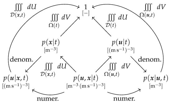
Figure 1. Relational diagram between the pdfs defined in this study [26].

3.2. Fluid Densities

The family of five pdfs are now used to define corresponding fluid mass densities, four of which are not usually encountered in the analysis of fluid flow systems:

(a)

A volumetric fluid density $\rho :\Omega \times \mathbb{R}\to {\mathbb{R}}_0^{+}$, $(\mathit{x},t)\mapsto \rho (\mathit{x},t)$ [kg m⁻³];

(b)

A velocimetric fluid density $Д:\mathcal{D}\times \mathbb{R}\to {\mathbb{R}}_0^{+}$, $(\mathit{u},t)\mapsto Д(\mathit{u},t)$ [kg (m s⁻¹)⁻³];

(c)

A velocivolumetric (phase space) fluid density $\zeta :\mathcal{D}\times \Omega \times \mathbb{R}\to {\mathbb{R}}_0^{+}$, $(\mathit{u},\mathit{x},t)\mapsto \zeta (\mathit{u},\mathit{x},t)$ [kg m⁻³ (m s⁻¹)⁻³];

(d)

A conditional velocimetric fluid density $\eta :\mathcal{D}\times \Omega \times \mathbb{R}\to {\mathbb{R}}_0^{+}$, $(\mathit{u},\mathit{x},t)\mapsto \eta (\mathit{u},\mathit{x},t)$ [kg (m s⁻¹)⁻³]; and

(e)

A conditional volumetric fluid density $\xi :\mathcal{D}\times \Omega \times \mathbb{R}\to {\mathbb{R}}_0^{+}$, $(\mathit{u},\mathit{x},t)\mapsto \xi (\mathit{u},\mathit{x},t)$ [kg m⁻³];

The density $Д$ uses the Cyrillic “de” character, from the transliteration of “density”.

Considering a fluid volume of fixed fluid mass M, the five fluid densities are defined to satisfy the following nine relations analogous to (1):

$$\begin{array}{cccc}\hfill M& ={\int \int \int }_{\Omega \left(t\right)}\rho (\mathit{x},t)dV,\hfill & \hfill M& ={\int \int \int }_{\mathcal{D}\left(t\right)}Д(\mathit{u},t)dU,\hfill \\ \hfill M& ={\int \int \int }_{\Omega \left(t\right)}{\int \int \int }_{\mathcal{D}(\mathit{x},t)}\zeta (\mathit{u},\mathit{x},t)dUdV\hfill & \hfill ={\int \int \int }_{\mathcal{D}\left(t\right)}& {\int \int \int }_{\Omega (\mathit{u},t)}\zeta (\mathit{u},\mathit{x},t)dVdU,\hfill \\ \hfill \rho (\mathit{x},t)& ={\int \int \int }_{\mathcal{D}(\mathit{x},t)}\zeta (\mathit{u},\mathit{x},t)dU,\hfill & \hfill Д(\mathit{u},t)& ={\int \int \int }_{\Omega (\mathit{u},t)}\zeta (\mathit{u},\mathit{x},t)dV,\hfill \\ \hfill \eta (\mathit{u},\mathit{x},t)& =\frac{\zeta (\mathit{u},\mathit{x},t)M}{\rho (\mathit{x},t)},\hfill & \hfill \xi (\mathit{u},\mathit{x},t)& =\frac{\zeta (\mathit{u},\mathit{x},t)M}{Д(\mathit{u},t)},\hfill \\ \hfill M& ={\int \int \int }_{\mathcal{D}(\mathit{x},t)}\eta (\mathit{u},\mathit{x},t)dU,\hfill & \hfill M& ={\int \int \int }_{\Omega (\mathit{u},t)}\xi (\mathit{u},\mathit{x},t)dV\hfill \end{array}$$

(2)

The integration pathways between the fluid densities are illustrated in the relational diagram in Figure 2.

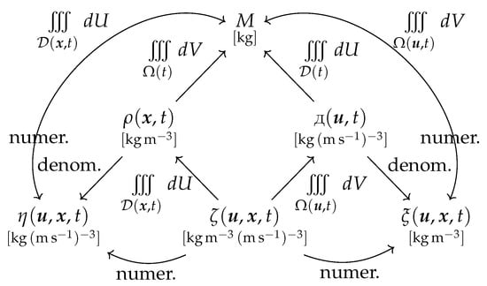
Figure 2. Relational diagram between the fluid densities defined in this study [26].

In studies of multiphase systems such as flow in porous media, the definition of Eulerian continuum variables is complicated by the presence of phase boundaries, which break the continuum assumption. To address this, numerous authors define an expected local fluid density $[\rho (\mathit{x},t\left)\right]$ by integration of the density $\rho (\mathit{x}+\mathit{r},t)$ multiplied by a weighting function $w(\mathit{r},t)$ over a small finite fluid volume $\mathcal{V}(\mathit{r},t)$, where $[·]$ is the volumetric expectation and $\mathit{r}\in \Omega$ is the local coordinate vector (e.g., [28,29,30]). This avoids the problems caused by taking a fluid volume to its infinitesimal limit. The weighting function $w(\mathit{r},t)$ satisfies the properties of the pdf $p\left(\mathit{r}\right|t)$, and is here formally identified as such. From this insight, and also considering a small velocimetric domain $\mathcal{U}$ with local coordinate $\mathit{s}\in \mathcal{D}$ for velocity averaging, as well as the small fluid mass domain $\mathsf{m}$ in either representation, the five fluid densities can be defined from their underlying pdfs by the convolutions:

$$\begin{array}{cc}\hfill [\rho ](\mathit{x},t)& ={\int }_{\mathsf{m}(\mathit{x},t)}p\left(\mathit{r}\right|t)dm(\mathit{x}+\mathit{r},t)={\int \int \int }_{\mathcal{V}(\mathit{x},t)}p\left(\mathit{r}\right|t)\rho (\mathit{x}+\mathit{r},t)dV(\mathit{r},t)\hfill \\ \hfill ⟨Д⟩(\mathit{u},t)& ={\int }_{\mathsf{m}(\mathit{u},t)}p\left(\mathit{s}\right|t)dm(\mathit{u}+\mathit{s},t)={\int \int \int }_{\mathcal{U}(\mathit{u},t)}p\left(\mathit{s}\right|t)Д(\mathit{u}+\mathit{s},t)dU(\mathit{s},t)\hfill \\ \hfill [⟨\zeta ⟩](\mathit{u},\mathit{x},t)& ={\int }_{\mathsf{m}(\mathit{u},\mathit{x},t)}p(\mathit{s},\mathit{r}|t)dm(\mathit{u}+\mathit{s},\mathit{x}+\mathit{r},t)\hfill \\ \hfill & ={\int \int \int }_{\mathcal{V}(\mathit{x},t)}{\int \int \int }_{\mathcal{U}(\mathit{u},\mathit{x}+\mathit{r},t)}p(\mathit{s},\mathit{r}|t)\zeta (\mathit{u}+\mathit{s},\mathit{x}+\mathit{r},t)dU(\mathit{s},\mathit{x}+\mathit{r},t)dV(\mathit{s},\mathit{r},t)\hfill \\ \hfill & ={\int \int \int }_{\mathcal{U}(\mathit{u},t)}{\int \int \int }_{\mathcal{V}(\mathit{u}+\mathit{s},\mathit{x},t)}p(\mathit{s},\mathit{r}|t)\zeta (\mathit{u}+\mathit{s},\mathit{x}+\mathit{r},t)dV(\mathit{u}+\mathit{s},\mathit{r},t)dU(\mathit{s},\mathit{r},t)\hfill \\ \hfill ⟨\eta ⟩(\mathit{u},\mathit{x},t)& ={\int }_{\mathsf{m}(\mathit{u},\mathit{x},t)}p\left(\mathit{s}\right|\mathit{x},t)dm(\mathit{u}+\mathit{s},\mathit{x},t)={\int \int \int }_{\mathcal{U}(\mathit{u},\mathit{x},t)}p\left(\mathit{s}\right|\mathit{x},t)\eta (\mathit{u}+\mathit{s},\mathit{x},t)dU(\mathit{s},\mathit{x},t)\hfill \\ \hfill \left[\xi \right](\mathit{u},\mathit{x},t)& ={\int }_{\mathsf{m}(\mathit{u},\mathit{x},t)}p\left(\mathit{r}\right|\mathit{u},t)dm(\mathit{u},\mathit{x}+\mathit{r},t)={\int \int \int }_{\mathcal{V}(\mathit{u},\mathit{x},t)}p\left(\mathit{r}\right|\mathit{u},t)\xi (\mathit{u},\mathit{x}+\mathit{r},t)dV(\mathit{u},\mathit{r},t)\hfill \end{array}$$

(3)

where $⟨·⟩$ is a local velocimetric expectation, and $dm$ is an infinitesimal element of fluid mass. Note that if each pdf is assumed uniformly distributed over its domain, each expected fluid density reduces to the product of its underlying pdf and the fluid mass, as required by dimensional considerations. The expectation notations in (3) are now dropped.

3.3. Generalized Densities

Using the generalized fluid densities, we can construct five generalized densities of any conserved extensive quantity carried by a fluid:

(a)

Volumetric densities $\alpha :\Omega \times \mathbb{R}\to {\mathbb{R}}_0^{+}$, $(\mathit{x},t)\mapsto \alpha (\mathit{x},t)$ [qty m⁻³];

(b)

Velocimetric densities $\beta :\mathcal{D}\times \mathbb{R}\to {\mathbb{R}}_0^{+}$, $(\mathit{u},t)\mapsto \beta (\mathit{u},t)$ [qty (m s⁻¹)⁻³];

(c)

Velocivolumetric (phase space) densities $\phi :\mathcal{D}\times \Omega \times \mathbb{R}\to {\mathbb{R}}_0^{+}$, $(\mathit{u},\mathit{x},t)\mapsto \phi (\mathit{u},\mathit{x},t)$ [qty m⁻³ (m s⁻¹)⁻³];

(d)

Conditional velocimetric densities $\theta :\mathcal{D}\times \Omega \times \mathbb{R}\to {\mathbb{R}}_0^{+}$, $(\mathit{u},\mathit{x},t)\mapsto \theta (\mathit{u},\mathit{x},t)$ [qty (m s⁻¹)⁻³]; and

(e)

Conditional volumetric densities $ϵ:\mathcal{D}\times \Omega \times \mathbb{R}\to {\mathbb{R}}_0^{+}$, $(\mathit{u},\mathit{x},t)\mapsto ϵ(\mathit{u},\mathit{x},t)$ [qty m⁻³];

where “qty” denotes the units of the conserved quantity. These are defined by the relations:

$$\begin{array}{cccc}\hfill \alpha (\mathit{x},t)& =\rho (\mathit{x},t)\underline{\alpha }(\mathit{x},t),\hfill & \hfill \beta (\mathit{u},t)& =Д(\mathit{u},t)\breve{\beta }(\mathit{u},t),\hfill \\ \hfill \phi (\mathit{u},\mathit{x},t)& =\zeta (\mathit{u},\mathit{x},t)\underline{\breve{\phi }}(\mathit{u},\mathit{x},t),\hfill & \hfill \theta (\mathit{u},\mathit{x},t)& =\eta (\mathit{u},\mathit{x},t)\underline{\breve{\theta }}(\mathit{u},\mathit{x},t),\hfill \\ \hfill ϵ(\mathit{u},\mathit{x},t)& =\xi (\mathit{u},\mathit{x},t)\underline{\breve{ϵ}}(\mathit{u},\mathit{x},t)\hfill \end{array}$$

(4)

where $\underline{\alpha }$, $\breve{\beta }$, $\underline{\breve{\phi }}$, $\underline{\breve{\theta }}$ and $\underline{\breve{ϵ}}$ [qty kg⁻¹] are specific densities, representing the quantity carried per unit fluid mass. For precision, these are labeled by an underline to indicate position dependence (a function of $\mathit{x}$), or a breve accent to indicate velocity dependence (a function of $\mathit{u}$). However, the fluid velocity $\mathit{u}$ does not require these designations, being already velocity-dependent.

The family of generalized densities will satisfy a set of integral relations analogous to (2), equating to the total integrated quantity $Q\left(t\right)$ [qty] rather than the total fluid mass M. The integral connections between generalized densities can also be plotted in a relational diagram analogous to Figure 2.

4. The Generalized Reynolds Transport Theorem and Example Systems

Recently, a generalized extension of the Reynolds transport theorem was presented for the multivariate mapping of the density of a conserved quantity in a generic coordinate space, induced by a vector or tensor field [24]. For the generalized density $\psi$ of a conserved quantity in an n-dimensional domain $\Omega$ within an n-dimensional space $\mathsf{M}$, described by the global Cartesian coordinate vector $\mathit{X}\subset {\mathbb{R}}^n$ and parameter vector $\mathit{C}\subset {\mathbb{R}}^m$, this reduces to:

$$\begin{array}{c}\hfill \begin{array}{cc}\hfill d\underset{\Omega \left(\mathit{C}\right)}{\int }\psi d^n\mathit{X}& =\left[{\nabla }_{\mathit{C}}\underset{\Omega \left(\mathit{C}\right)}{\int }\psi d^n\mathit{X}\right]·d\mathit{C}=\left[\underset{\Omega \left(\mathit{C}\right)}{\int }\left[{\nabla }_{\mathit{C}}\psi +{\nabla }_{\mathit{X}}·\left(\psi \mathit{V}\right)\right]d^n\mathit{X}\right]·d\mathit{C},\hfill \end{array}\end{array}$$

(5)

where $\mathit{V}={\left({\nabla }_{\mathit{C}}\mathit{X}\right)}^{\top }$ is a smooth vector or tensor field (a function of $\mathit{C}$), ${\nabla }_{\mathit{X}}$ is the gradient with respect to $\mathit{X}$, ${\nabla }_{\mathit{C}}$ is the gradient with respect to $\mathit{C}$, and $d^n\mathit{X}$ is a volume element in $\Omega$. This is applicable to all spaces containing the density field $\psi (\mathit{V},\mathit{C})$ of a conserved quantity, not just the volumetric spaces usually considered in fluid mechanics.

We now apply (5) to three example formulations, also reported in [26]. In the following, we adopt the following specific quantities in (4): specific mass of fluid 1 [–], specific mass ${\chi }_c$ of chemical species c [kg${}_c$ kg${}^{-1}$], specific linear momentum (fluid velocity) $\mathit{u}$ [m s${}^{-1}$], specific angular momentum $\mathfrak{r}\times \mathit{u}$ [m${}^2$ s${}^{-1}$] (where $\mathfrak{r}$ is the local lever arm radius [m]), specific energy e [J kg${}^{-1}$], specific charge z [C kg${}^{-1}$] and specific entropy s [J K${}^{-1}$ kg${}^{-1}$]. We also use the following terms: rate of change of mass ${\dot{M}}_c$ of species c, total force $\sum \mathit{F}$, total torque $\sum \mathit{T}$, total energy E, heat flow rate ${\dot{Q}}_{in}$, rate of work ${\dot{W}}_{in}$, total charge Z, electrical current I, charge $z_c$ on species c, total entropy S, entropy production $\dot{\sigma }$ and non-fluid entropy flow rate ${\dot{S}}^{nf}$.

4.1. Volumetric-Temporal Formulation

Consider the traditional example of a volumetric space $\Omega$ with coordinates $\mathit{X}=\mathit{x}$, time parameter $\mathit{C}=t$ and generalized density $\alpha (\mathit{x},t)=\rho (\mathit{x},t)\underline{\alpha }(\mathit{x},t)$. The field is $\mathit{V}=\partial \mathit{x}/\partial t=\mathit{u}$, the velocity field. Equation (5) gives:

$$\frac{DQ}{Dt}=\frac{dQ}{dt}=\frac{d}{dt}\underset{\Omega \left(t\right)}{\int \int \int }\alpha dV=\underset{\Omega \left(t\right)}{\int \int \int }\left[\frac{\partial \alpha }{\partial t}+{\nabla }_{\mathit{x}}·\left(\alpha \mathit{u}\right)\right]dV$$

(6)

where $D/Dt$ is the substantial or material derivative, in this case equivalent to the total derivative $d/dt$. Equation (6) is the standard Reynolds transport theorem [1,2,3,8,9]. The integral conservation laws obtained from (6) are listed in Table 1 (e.g., [2,3,4,5,6,7]).

Table 1. Conservation Laws for the Volumetric-Temporal Formulation [2,3,4,5,6,7].

Conserved Quantity	Density $\mathbf{=}\mathit{\rho }\underset{-}{\mathit{\alpha }}$	Integral Equation
Fluid mass	$\rho$	0	$=\underset{\Omega \left(t\right)}{\int \int \int }\left[{\displaystyle \frac{\partial \rho }{\partial t}}+{\nabla }_{\mathit{x}}·(\rho \mathit{u})\right]dV$
Species mass	$\rho {\underline{\chi }}_c$	${\dot{M}}_c$	$=\underset{\Omega \left(t\right)}{\int \int \int }\left[{\displaystyle \frac{\partial \rho {\underline{\chi }}_c}{\partial t}}+{\nabla }_{\mathit{x}}·(\rho {\underline{\chi }}_c\mathit{u})\right]dV$
Linear momentum	$\rho \mathit{u}$	$\sum \mathit{F}$	$=\underset{\Omega \left(t\right)}{\int \int \int }\left[{\displaystyle \frac{\partial \rho \mathit{u}}{\partial t}}+{\nabla }_{\mathit{x}}·(\rho \mathit{u}\mathit{u})\right]dV$
Angular momentum	$\rho (\underline{\mathfrak{r}}\times \mathit{u})$	$\sum \mathit{T}$	$=\underset{\Omega \left(t\right)}{\int \int \int }\left[{\displaystyle \frac{\partial \rho (\underline{\mathfrak{r}}\times \mathit{u})}{\partial t}}+{\nabla }_{\mathit{x}}·(\rho (\underline{\mathfrak{r}}\times \mathit{u})\mathit{u})\right]dV$
Energy	$\rho \underline{e}$	${\displaystyle \frac{DE}{Dt}}={\dot{Q}}_{in}+{\dot{W}}_{in}$	$=\underset{\Omega \left(t\right)}{\int \int \int }\left[{\displaystyle \frac{\partial \rho \underline{e}}{\partial t}}+{\nabla }_{\mathit{x}}·(\rho \underline{e}\mathit{u})\right]dV$
Charge (in solution)	$\rho \underline{z}$	${\displaystyle \frac{DZ}{Dt}}=I+{\sum }_c{z}_c{\dot{M}}_c$	$=\underset{\Omega \left(t\right)}{\int \int \int }\left[{\displaystyle \frac{\partial \rho \underline{z}}{\partial t}}+{\nabla }_{\mathit{x}}·(\rho \underline{z}\mathit{u})\right]dV$
Entropy	$\rho \underline{s}$	${\displaystyle \frac{DS}{Dt}}=\dot{\sigma }$$+{\dot{S}}^{nf}$	$=\underset{\Omega \left(t\right)}{\int \int \int }\left[{\displaystyle \frac{\partial \rho \underline{s}}{\partial t}}+{\nabla }_{\mathit{x}}·(\rho \underline{s}\mathit{u})\right]dV$

4.2. Velocimetric-Temporal Formulation

Consider a velocimetric space $\mathcal{D}$ with coordinates $\mathit{X}=\mathit{u}$, time parameter $\mathit{C}=t$ and generalized density $\beta (\mathit{u},t)=Д(\mathit{u},t)\breve{\beta }(\mathit{u},t)$. The field is $\mathit{V}=\partial \mathit{u}/\partial t=\dot{\mathit{u}}$, the local acceleration vector field. Equation (5) gives:

$$\begin{array}{c}\hfill \begin{array}{c}\hfill \frac{DQ}{Dt}=\frac{dQ}{dt}=\frac{d}{dt}\underset{\mathcal{D}\left(t\right)}{\int \int \int }\beta dU=\underset{\mathcal{D}\left(t\right)}{\int \int \int }\left[\frac{\partial \beta }{\partial t}+{\nabla }_{\mathit{u}}·\left(\beta \dot{\mathit{u}}\right)\right]dU\end{array}\end{array}$$

(7)

Equation (7) provides a new velocimetric-temporal formulation of the Reynolds transport theorem [24]. The integral conservation laws obtained from (7) for the seven conserved quantities are listed in Table 2. Since these integrals are equal to the total rate of change of the conserved quantity $dQ/dt$, they equate to the same source-sink terms as for the volumetric-temporal formulation (Table 1).

Table 2. Conservation Laws for the Velocimetric-Temporal Formulation.

Conserved Quantity	Density $\mathbf{=}Д\stackrel{\mathbf{˘}}{\mathit{\beta }}$	Integral Equation
Fluid mass	$Д$	0	$=\underset{\mathcal{D}\left(t\right)}{\int \int \int }\left[{\displaystyle \frac{\partial Д}{\partial t}}+{\nabla }_{\mathit{u}}·(Д\dot{\mathit{u}})\right]dU$
Species mass	$Д{\breve{\chi }}_c$	${\dot{M}}_c$	$=\underset{\mathcal{D}\left(t\right)}{\int \int \int }\left[{\displaystyle \frac{\partial Д{\breve{\chi }}_c}{\partial t}}+{\nabla }_{\mathit{u}}·(Д{\breve{\chi }}_c\dot{\mathit{u}})\right]dU$
Linear momentum	$Д\mathit{u}$	$\sum \mathit{F}$	$=\underset{\mathcal{D}\left(t\right)}{\int \int \int }\left[{\displaystyle \frac{\partial Д\mathit{u}}{\partial t}}+{\nabla }_{\mathit{u}}·(Д\mathit{u}\dot{\mathit{u}})\right]dU$
Angular momentum	$Д(\breve{\mathfrak{r}}\times \mathit{u})$	$\sum \mathit{T}$	$=\underset{\mathcal{D}\left(t\right)}{\int \int \int }\left[{\displaystyle \frac{\partial Д(\breve{\mathfrak{r}}\times \mathit{u})}{\partial t}}+{\nabla }_{\mathit{u}}·(Д(\breve{\mathfrak{r}}\times \mathit{u})\dot{\mathit{u}})\right]dU$
Energy	$Д\breve{e}$	${\displaystyle \frac{DE}{Dt}}={\dot{Q}}_{in}+{\dot{W}}_{in}$	$=\underset{\mathcal{D}\left(t\right)}{\int \int \int }\left[{\displaystyle \frac{\partial Д\breve{e}}{\partial t}}+{\nabla }_{\mathit{u}}·(Д\breve{e}\dot{\mathit{u}})\right]dU$
Charge (in solution)	$Д\breve{z}$	${\displaystyle \frac{DZ}{Dt}}=I+{\sum }_c{z}_c{\dot{M}}_c$	$=\underset{\mathcal{D}\left(t\right)}{\int \int \int }\left[{\displaystyle \frac{\partial Д\breve{z}}{\partial t}}+{\nabla }_{\mathit{u}}·(Д\breve{z}\dot{\mathit{u}})\right]dU$
Entropy	$Д\breve{s}$	${\displaystyle \frac{DS}{Dt}}=\dot{\sigma }$$+{\dot{S}}^{nf}$	$=\underset{\mathcal{D}\left(t\right)}{\int \int \int }\left[{\displaystyle \frac{\partial Д\breve{s}}{\partial t}}+{\nabla }_{\mathit{u}}·(Д\breve{s}\dot{\mathit{u}})\right]dU$

4.3. Time-Independent Velocimetric-Spatial Formulation

Finally, consider a time-independent velocivolumetric space $\mathcal{D}\times \Omega$ with velocity coordinates $\mathit{X}=\mathit{u}$, spatial parameter $\mathit{C}=\mathit{x}$ and generalized density $\phi (\mathit{u},\mathit{x})=\zeta (\mathit{u},\mathit{x})\underline{\breve{\phi }}(\mathit{u},\mathit{x})$. The field is $\mathit{V}={\left({\nabla }_{\mathit{x}}\mathit{u}\right)}^{\top }={\mathit{G}}^{\top }$, the velocity gradient tensor field. Equation (5) gives:

$$\begin{array}{c}\hfill \begin{array}{cc}\hfill {\nabla }_{\mathit{x}}\alpha & ={\nabla }_{\mathit{x}}\underset{\mathcal{D}\left(\mathit{x}\right)}{\int \int \int }\phi dU=\underset{\mathcal{D}\left(\mathit{x}\right)}{\int \int \int }\left[{\nabla }_{\mathit{x}}\phi +{\nabla }_{\mathit{u}}·\left(\phi {\mathit{G}}^{\top }\right)\right]dU\hfill \end{array}\end{array}$$

(8)

The integral conservation laws obtained from (8) for the seven identified conserved quantities are listed in Table 3. These relations are of different character to those in Table 1 and Table 2, giving new expressions for the spatial gradient of each generalized density $\alpha =\rho \underline{\alpha }$.

Table 3. Conservation Laws for the Time-Independent Velocimetric-Spatial Formulation.

Conserved Quantity	Density $\mathbf{=}\mathit{\zeta }\stackrel{\mathbf{˘}}{\underset{-}{\mathit{\phi }}}$	Integral Equation
Fluid mass	$\zeta$	${\nabla }_{\mathit{x}}\rho$	$=\underset{\mathcal{D}\left(\mathit{x}\right)}{\int \int \int }\left({\nabla }_{\mathit{x}}\zeta +{\nabla }_{\mathit{u}}·\left(\zeta {\mathit{G}}^{\top }\right)\right)dU$
Species mass	$\zeta {\breve{\underline{\chi }}}_c$	${\nabla }_{\mathit{x}}(\rho {\underline{\chi }}_c)$	$=\underset{\mathcal{D}\left(\mathit{x}\right)}{\int \int \int }\left({\nabla }_{\mathit{x}}\left(\zeta {\breve{\underline{\chi }}}_c\right)+{\nabla }_{\mathit{u}}·\left(\zeta {\breve{\underline{\chi }}}_c{\mathit{G}}^{\top }\right)\right)dU$
Linear momentum	$\zeta \mathit{u}$	${\nabla }_{\mathit{x}}(\rho \mathit{u})$	$=\underset{\mathcal{D}\left(\mathit{x}\right)}{\int \int \int }\left({\nabla }_{\mathit{x}}\left(\zeta \mathit{u}\right)+{\nabla }_{\mathit{u}}·\left(\zeta \mathit{u}{\mathit{G}}^{\top }\right)\right)dU$
Angular momentum	$\zeta (\underline{\breve{\mathfrak{r}}}\times \mathit{u})$	${\nabla }_{\mathit{x}}(\rho (\underline{\mathfrak{r}}\times \mathit{u}))$	$=\underset{\mathcal{D}\left(\mathit{x}\right)}{\int \int \int }\left({\nabla }_{\mathit{x}}\left(\zeta (\underline{\breve{\mathfrak{r}}}\times \mathit{u})\right)+{\nabla }_{\mathit{u}}·\left(\zeta (\underline{\breve{\mathfrak{r}}}\times \mathit{u}){\mathit{G}}^{\top }\right)\right)dU$
Energy	$\zeta \breve{\underline{e}}$	${\nabla }_{\mathit{x}}(\rho \underline{e})$	$=\underset{\mathcal{D}\left(\mathit{x}\right)}{\int \int \int }\left({\nabla }_{\mathit{x}}\left(\zeta \breve{\underline{e}}\right)+{\nabla }_{\mathit{u}}·\left(\zeta \breve{\underline{e}}{\mathit{G}}^{\top }\right)\right)dU$
Charge (in solution)	$\zeta \breve{\underline{z}}$	${\nabla }_{\mathit{x}}(\rho \underline{z})$	$=\underset{\mathcal{D}\left(\mathit{x}\right)}{\int \int \int }\left({\nabla }_{\mathit{x}}\left(\zeta \breve{\underline{z}}\right)+{\nabla }_{\mathit{u}}·\left(\zeta \breve{\underline{z}}{\mathit{G}}^{\top }\right)\right)dU$
Entropy	$\zeta \breve{\underline{s}}$	${\nabla }_{\mathit{x}}(\rho \underline{s})$	$=\underset{\mathcal{D}\left(\mathit{x}\right)}{\int \int \int }\left({\nabla }_{\mathit{x}}\left(\zeta \breve{\underline{s}}\right)+{\nabla }_{\mathit{u}}·\left(\zeta \breve{\underline{s}}{\mathit{G}}^{\top }\right)\right)dU$

5. Conclusions

This study examines the formulation of different fluid densities required by a generalized Reynolds transport theorem for different coordinate spaces [24], based on a velocivolumetric Eulerian description of fluid flow. The family of five pdfs $p(\mathit{u},\mathit{x}|t)$, $p\left(\mathit{x}\right|t)$, $p\left(\mathit{u}\right|t)$, $p\left(\mathit{u}\right|\mathit{x},t)$ and $p\left(\mathit{x}\right|\mathit{u},t)$ are used by convolution to define corresponding fluid densities $\zeta (\mathit{u},\mathit{x},t),\rho (\mathit{x},t),(\mathit{u},t),\eta (\mathit{u},\mathit{x},t)$ and $\xi (\mathit{u},\mathit{x},t)$. These in turn can be used with specific quantities to define generalized densities of any conserved quantity in the fluid. Applying these densities within the extended Reynolds framework, we derive new families of integral conservation laws for seven important conserved quantities in the volumetric, velocimetric and time-independent velocivolumetric formulations. The analyses substantially expand the scope of known conservation laws for the analysis of fluid flow systems.

References

- Reynolds, O. Papers on Mechanical and Physical Subjects; Cambridge University Press: Cambridge, UK, 1903; Volume III. [Google Scholar]
- White, F.M. Fluid Mechanics, 2nd ed.; McGraw-Hill Higher Education: New York, NY, USA, 1986. [Google Scholar]
- Munson, B.R.; Young, D.F.; Okiishi, T.H.; Huebsch, W.W. Fundamentals of Fluid Mechanics, 6th ed.; John Wiley: Hoboken, NJ, USA, 2010. [Google Scholar]
- De Groot, S.R.; Mazur, P. Non-Equilibrium Thermodynamics; Dover Publicatiions: Mignola, NY, USA, 1984. [Google Scholar]
- Bird, R.B.; Stewart, W.E.; Lightfoot, E.N. Transport Phenomena, 2nd ed.; John Wiley & Sons: New York, NY, USA, 2006. [Google Scholar]
- White, F.M. Viscous Fluid Flow, 3rd ed.; McGraw-Hill: New York, NY, USA, 2006. [Google Scholar]
- Durst, F. Fluid Mechanics; Springer: Berlin, Germany, 2008. [Google Scholar]
- Dvorkin, E.N.; Goldschmit, M.B. Nonlinear Continua; Springer: Berlin, Germany, 2006. [Google Scholar]
- Truesdell, C.; Toupin, R.A. The classical field theories. In Handbuch der Physik, Band III/1; Flügge, S., Ed.; Springer: Berlin, Germany, 1960; p. 347. [Google Scholar]
- Seguin, B.; Hinz, D.F.; Fried, E. Extending the transport theorem to rough domains of integration. Appl. Mech. Rev. 2014, 66, 050802. [Google Scholar] [CrossRef] [PubMed]
- Falach, L.; Segev, R. Reynolds transport theorem for smooth deformations of currents on manifolds. Math. Mech. Solids 2015, 20, 770–786. [Google Scholar] [CrossRef][Green Version]
- Gurtin, M.E.; Struthers, A.; Williams, W.O. A transport theorem for moving interfaces. Q. Appl. Math. 1989, 47, 773–777. [Google Scholar] [CrossRef]
- Ochoa-Tapia, J.A.; del Rio, J.A.; Whitaker, S. Bulk and surface diffusion in porous media: An application of the surface-averaging theorem. Chem. Eng. Sci. 1993, 48, 2061–2082. [Google Scholar] [CrossRef]
- Slattery, J.C.; Sagis, L.; Oh, E.-S. Interfacial Transport Phenomena, 2nd ed.; Springer: New York, NY, USA, 2007. [Google Scholar]
- Fosdick, R.; Tang, H. Surface transport in continuum mechanics. Math. Mech. Solids 2009, 14, 587–598. [Google Scholar] [CrossRef]
- Lidström, P. Moving regions in Euclidean space and Reynolds transport theorem. Math. Mech. Solids 2011, 16, 366–380. [Google Scholar] [CrossRef]
- Flanders, H. Differentiation under the integral sign. Am. Mon. 1973, 80, 615–627. [Google Scholar] [CrossRef]
- Frankel, T. The Geometry of Physics, 3rd ed.; Cambridge University Press: Cambridge, UK, 2013. [Google Scholar]
- Harrison, J. Operator calculus of differential chains and differential forms. J. Geom. Anal. 2015, 25, 357–420. [Google Scholar] [CrossRef][Green Version]
- Anderson, T.B.; Jackson, R. A fluid mechanical description of fluidized beds. Ind. Eng. Chem. Fund. 1967, 6, 527–539. [Google Scholar] [CrossRef]
- Whitaker, S. Diffusion and dispersion in porous media. AIChE J. 1967, 13, 420–427. [Google Scholar] [CrossRef]
- Slattery, J.C. Flow of viscoelastic fluids through porous media. AIChE J. 1967, 13, 1067–1071. [Google Scholar] [CrossRef]
- Marle, C.M. Écoulements monophasiques en milieu poreux. Rev. L’Inst. Franç. Pét. 1967, 22, 1471–1509. [Google Scholar]
- Niven, R.K.; Cordier, L.; Kaiser, E.; Schlegel, M.; Noack, B.R. Rethinking the Reynolds transport theorem, Liouville equation, and Perron-Frobenius and Koopman operators. arXiv 2020, arXiv:1810.06022. [Google Scholar]
- Niven, R.K.; Cordier, L.; Kaiser, E.; Schlegel, M.; Noack, B.R. New conservation laws based on generalized Reynolds transport theorems. In Proceedings of the 22nd Australasian Fluid Mechanics Conference AFMC2020, Brisbane, Australia, 7–10 December 2020; p. 110. [Google Scholar]
- Niven, R.K. A hierarchy of probability, fluid and generalized densities for the Eulerian velocivolumetric description of fluid flow, for new families of conservation laws. Entropy 2022, 24, 1493. [Google Scholar] [CrossRef]
- Jaynes, E.T. Probability Theory: The Logic of Science; Bretthorst, G.L., Ed.; Cambridge University Press: Cambridge, UK, 2003. [Google Scholar]
- Matheron, G. Les variables régionalisées et leur estimation, une application de la théorie de fonctions aléatoires aux sciences de la nature; Masson et Cie: Paris, France, 1965. (In French) [Google Scholar]
- Monin, A.S.; Yaglom, A.M. Statistical Fluid Mechanics: Mechanics of Turbulence; Dover Publications: Mignola, NY, USA, 1971. [Google Scholar]
- Cushman, J.H. On unifying the concepts of scale, instrumentation, and stochastics in the development of multiphase transport theory. Water Resour. Res. 1984, 20, 1668–1676. [Google Scholar] [CrossRef]
Publisher’s Note: MDPI stays neutral with regard to jurisdictional claims in published maps and institutional affiliations. |
© 2022 by the author. Licensee MDPI, Basel, Switzerland. This article is an open access article distributed under the terms and conditions of the Creative Commons Attribution (CC BY) license (https://creativecommons.org/licenses/by/4.0/).