Classification and Uncertainty Quantification of Corrupted Data Using Supervised Autoencoders ^†

Abstract

Parametric and non-parametric classifiers often have to deal with real-world data, where corruptions such as noise, occlusions, and blur are unavoidable. We present a probabilistic approach to classify strongly corrupted data and quantify uncertainty, even though the corrupted data do not have to be included to the training data. A supervised autoencoder is the underlying architecture. We used the decoding part as a generative model for realistic data and extended it by convolutions, masking, and additive Gaussian noise to describe imperfections. This constitutes a statistical inference task in terms of the optimal latent space activations of the underlying uncorrupted datum. We solved this problem approximately with Metric Gaussian Variational Inference (MGVI). The supervision of the autoencoder’s latent space allowed us to classify corrupted data directly under uncertainty with the statistically inferred latent space activations. We show that the derived model uncertainty can be used as a statistical “lie detector” of the classification. Independent of that, the generative model can optimally restore the corrupted datum by decoding the inferred latent space activations.

1. Introduction and Motivation

Many real-world applications of data-driven classifiers, e.g., neural networks, involve corruptions that pose significant challenges to the pretrained classifiers. Often, the corruption must previously be included, and, thus, already be known during training. For instance, noise (e.g., due to sensor imperfections) and convolutions (e.g., due to lens flares or unfocused images) are inevitable in image processing systems and may occur spontaneously and irregularly. The same holds for masking, which may occur when a foreign object occludes the actual object of interest (e.g., water droplets, dirt, or scratches on the camera lens). Hence, we aimed to answer the following question in this paper: How can we classify corrupted data with a parametric classifier without imposing any constraints on the training data? As classifying corrupted data naturally demands a measure of uncertainty for validation, we included both model uncertainty ${\mathit{\delta }}_m$ and reconstruction uncertainty ${\mathit{\delta }}_r$ in the classification. We refer to ${\mathit{\delta }}_m$ as the model’s confidence of the classification itself. In contrast, we refer to ${\mathit{\delta }}_r$ as the confidence of the process of reconstructing the latent space activations given some corrupted datum. An overview of the proposed method is illustrated in Figure 1.

2. Classification and Uncertainty Quantification of Corrupted Data

2.1. Methodology Overview and Related Work

To address the challenge of classification and uncertainty quantification of corrupted data, we propose the following core approach, illustrated in Figure 2.

① In the first step, we trained a supervised autoencoder [1] that is: (a) capable of classifying the input data with its latent space activations $\mathit{h}$ and (b) capable of decoding the (supervised) latent space activations to generate higher-dimensional data, targeting it to be identical to the input. Except for these two constraints ((a) and (b)), we did not impose any further restrictions on the autoencoder.

② In the second step, we decoupled the decoder g from the autoencoder and treated the decoder as a fixed generative function g. Neither retraining nor further modifying of g is performed in the following steps.

③ In the third step, we included g in an Additive White Gaussian Noise (AWGN) channel model $\mathit{d}=\mathit{m}\mathit{C}g\left(\mathit{h}\right)+\mathit{n}$. This AWGN channel model additionally involves heavy corruption such as convolution $\mathit{C}$ and masking $\mathit{m}$.

④ In the final step, we approximated the posterior probability distribution $\mathcal{P}\left(\mathit{h}\right|\mathit{d})$ in the latent space and derived the mean and standard deviation, corresponding optimally to some uncorrupted datum $g\left(\mathit{h}\right)$, given the corrupted datum $\mathit{d}$. Due to supervision in the latent space, this reconstruction enables a direct classification of $\mathit{d}$ including model and reconstruction uncertainty quantification, even though the decoding function was trained on uncorrupted data. We used a set of samples $\mathcal{H}$ from the approximate posterior probability distribution to determine the sample mean $\mathrm{mean}\left(\mathcal{H}\right)=\overline{\mathcal{H}}$, as well as the set’s reconstruction uncertainty ${\mathit{\delta }}_r$ with the sample standard deviation $\mathrm{std}\left(\mathcal{H}\right)$. Samples are statistically inferred by Metric Gaussian Variational Inference (MGVI) [2]. In addition to the reconstruction uncertainty ${\mathit{\delta }}_r$, we determined the model uncertainty by calculating the Mahalanobis distance (M-distance) in the latent space representation, slightly different from [3]. Here, we distinguish between reconstruction uncertainty ${\mathit{\delta }}_{\mathbf{r}}$ and model uncertainty ${\mathit{\delta }}_{\mathit{m}}$ to evaluate the confidence of the process of inferring $\mathit{h}$ and to evaluate the confidence of the classification given by the supervised latent space, respectively. Similar to our approach, references [4,5] showed that the reconstruction of the latent space by posterior inference and by using generative models [6,7,8] for a corrupted datum can lead to an optimal image restoration with uncertainty quantification. These methods do not, however, focus on classifying the corrupted datum in the latent space, nor do they use supervised autoencoder structures. In the field of quantifying uncertainties of classifications, several methods exist. Predominantly, Bayesian Neural Networks (BNNs) [9] and Monte Carlo dropout (MC-dropout) [10] have recently shown success. More recently, Evidential Deep Learning (EDL) [11] was introduced as yet another probabilistic method to quantify classification uncertainty. The latter two methods are compared to our method in Section 3. Finally, various methods to perform image restoration exist in the literature, such as the well-known denoising autoencoder [12]. These conventional methods require prior knowledge of the corruption to be included to the training data.

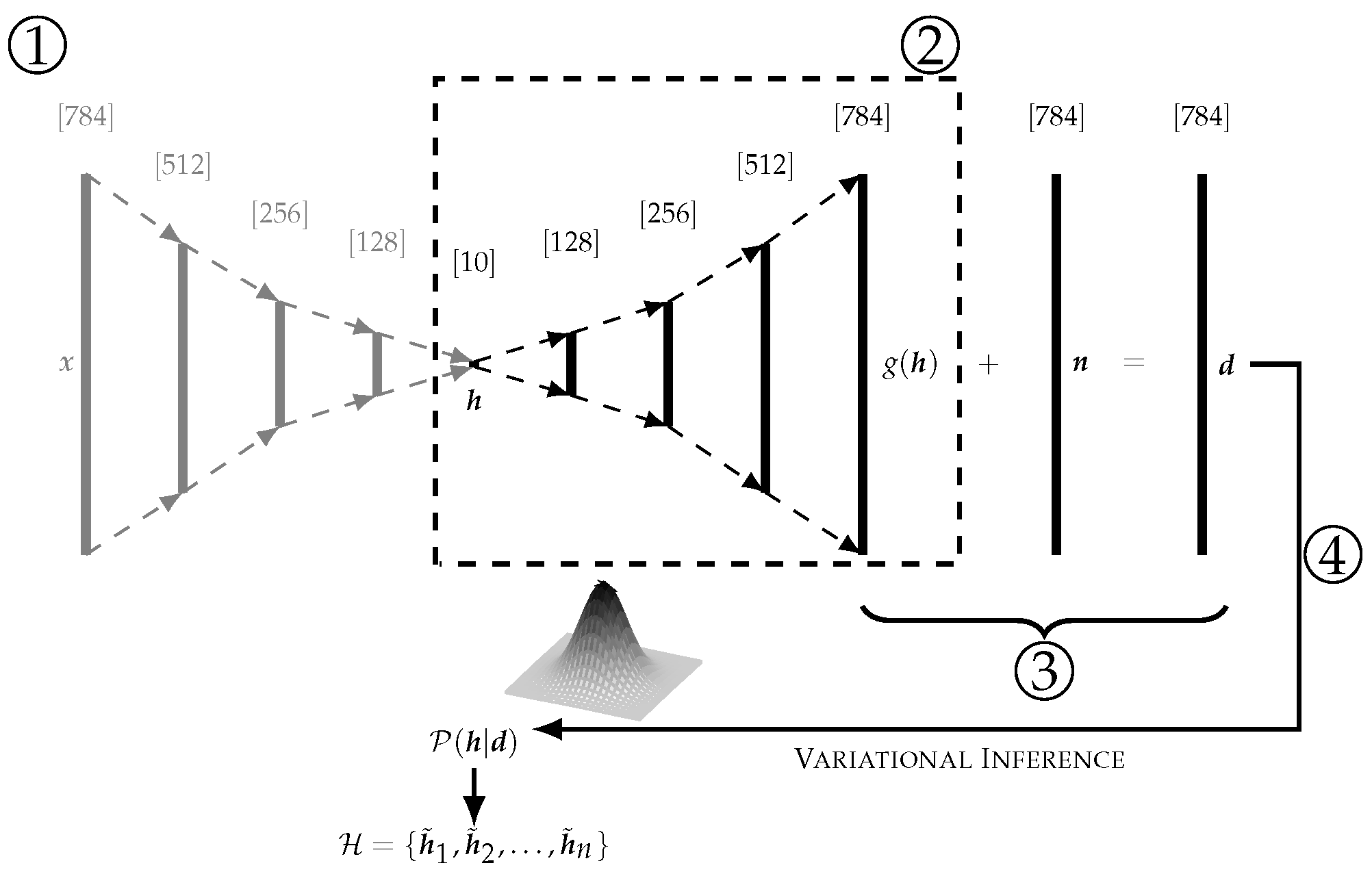
2.2. Generative Model and Bayesian Inference with Neural Networks

The first step of our method is to train a supervised autoencoder. The autoencoder involves the encoding function f (mapping data $\mathit{x}\in {\mathbb{R}}^p$ to the latent space representation with activations $\mathit{h}\in {\mathbb{R}}^z,z\in \mathbb{N}$), as well as the decoding function g (mapping $\mathit{h}$ to the data space representation $\widehat{\mathit{x}}\in {\mathbb{R}}^p,p\in \mathbb{N},p\gg z$). The parameters of $f:{\mathbb{R}}^p\to {\mathbb{R}}^z$ and $g:{\mathbb{R}}^z\to {\mathbb{R}}^p$ are optimized via a combination of two loss terms ${\mathcal{L}}_{gf}$ (representing the reconstruction loss in the data space) and ${\mathcal{L}}_f$ (representing the classification loss in the latent space):

$$\begin{array}{ll}{\mathcal{L}}_{\mathrm{SAE}}& ={\mathcal{L}}_{gf}(g\left(f\left(\mathit{x}\right)\right),\mathit{x})+{\mathcal{L}}_f(f{\left(\mathit{x}\right)}^j,\mathbf{y})\\ & ={\mathcal{L}}_{gf}(\widehat{\mathit{x}},\mathit{x})+{\mathcal{L}}_f({\mathit{h}}^j,\mathbf{y}),\end{array}$$

(1)

where j denotes the number of activations in the latent space $\mathit{h}$ that are supervised, i.e., ${\mathit{h}}^j=[{\mathit{h}}_1,\cdots ,{\mathit{h}}_j]$. After normalizing all data samples in the range of $[0,1]$, we used the corresponding cross-entropy for each respective loss term to penalize false classifications in the latent space and inaccurate reconstructions in the data space. Note that the loss term ${\mathcal{L}}_f({\mathit{h}}^j,\mathbf{y})$ processes activations from the latent space ${\mathit{h}}^j$ with the $\mathrm{softmax}$-function (i.e., ${\mathcal{L}}_{\mathrm{SAE}}={\mathcal{L}}_{gf}(\widehat{\mathit{x}},\mathit{x})+{\mathcal{L}}_f(\mathrm{softmax}\left({\mathit{h}}^j\right),\mathbf{y})$). The $\mathrm{softmax}$-function’s output yields values ranging from $[0,1]$, which can be penalized by one-hot-encoded labels $\mathbf{y}$. The $\mathrm{softmax}$-function is not included as an activation function in our neural network, where the latent space $\mathit{h}$ is activated linearly; see Section 3 for details. We minimized the general loss function of Equation (1) using the Adam optimizer [13] (test accuracy of $[98.6\%;89.4\%]$ on the encoding function f with [MNIST; Fashion-MNIST]). Once the training procedure converged, we decoupled the decoding function g from the autoencoder. Without loss of generality, we then used an AWGN model including the nonlinearity $g\left(\mathit{h}\right)$, which additionally involves masking $\mathit{m}$ and convolution $\mathit{C}$ on g:

$$\mathit{d}=\mathit{m}\mathit{C}g\left(\mathit{h}\right)+\mathit{n}.$$

(2)

Additive white Gaussian noise, $\mathit{n}\in {\mathbb{R}}^p\sim \mathcal{N}(0,{\Sigma }_n)$, is applied to the decoded latent space signal $g\left(\mathit{h}\right)$, which yields the corrupted data $\mathit{d}\in {\mathbb{R}}^p$. Note that, for the implementation of $\mathit{h}=\mathbf{A}\mathbf{\xi }+{\mathbf{\mu }}_h$, the reparametrization trick [14] is applied (${\Sigma }_{\mathit{h}}=\mathrm{cov}\left(f\left({\mathit{X}}_{\mathrm{Val}}\right)\right),{\Sigma }_{\mathit{h}}=\mathbf{A}{\mathbf{A}}^{\mathrm{T}}$, ${\Sigma }_{\mathit{h}}\in {\mathbb{R}}^{z\times z},\mathbf{\xi }\sim \mathcal{N}(\mathbf{0},\mathbf{I}),\mathbf{\xi }\in {\mathbb{R}}^z$, ${\mathbf{\mu }}_h=\mathrm{mean}\left({\mathit{X}}_{\mathrm{Val}}\right),{\mathbf{\mu }}_h\in {\mathbb{R}}^z$). In addition to AWGN, we included the corruptions of masking $\mathit{m}$ and convolutions $\mathit{C}$, which are both linear operations.

Since we are interested in reconstructing the latent space activation $\mathit{h}$ from $\mathit{d}$ alongside uncertainty quantification, the goal is to determine the posterior distribution $\mathcal{P}\left(\mathit{h}\right|\mathit{d})\propto \mathcal{P}\left(\mathit{d}\right|\mathit{h}\left)\mathcal{P}\right(\mathit{h})$. The log-probability distribution reads

$$-ln\mathcal{P}\left(\mathit{h}\right|\mathit{d})={\displaystyle \frac{1}{2}}\left({\left(\mathit{d}-\mathit{m}\mathit{C}g\left(\mathit{h}\right)\right)}^{\mathrm{T}}{\Sigma }_{\mathit{n}}^{-1}\left(\mathit{d}-\mathit{m}\mathit{C}g\left(\mathit{h}\right)\right)+\left({\mathit{h}}^{\mathrm{T}}{\Sigma }_{\mathit{h}}^{-1}\mathit{h}\right)\phantom{{\left(\mathit{h})\right)}^{\mathrm{T}}}\right)+\mathrm{const}.,$$

(3)

where ${(·)}^{\mathrm{T}}$ denotes the matrix transpose. Since we are ultimately interested in the analytically intractable mean of $\mathit{h},{〈\mathit{h}〉}_{\mathcal{P}\left(\mathit{h}\right|\mathit{d})}=\int \mathit{h}\mathcal{P}\left(\mathit{h}\right|\mathit{d})d\mathit{h}$, we approximately determined the mean and the variance of $\mathcal{P}\left(\mathit{h}\right|\mathit{d})$ by applying MGVI. Similar to other variational inference methods [14,15], MGVI approximates the distribution by a simpler, but tractable distribution from within a variational family, $\mathcal{Q}\left(\mathit{h}\right)$. The parameters of $\mathcal{Q}\left(\mathit{h}\right)$, i.e., mean $\eta$ and covariance $\Delta$, are obtained by minimizing the variational lower bound. The size of a full variational covariance scales quadratically with the number of latent variables. Taking these limitations into account, we employed MGVI, which locally approximates the target distribution using the inverse Fisher metric as an uncertainty estimate around the variational mean $\eta$, which we are optimizing for. The approximation is represented by an ensemble of samples $\mathcal{H}=\{{\tilde{\mathit{h}}}_1,{\tilde{\mathit{h}}}_2,\cdots ,{\tilde{\mathit{h}}}_n\}$ with $\tilde{\mathit{h}}\in {\mathbb{R}}^z$, which we used for our analysis. $\tilde{\mathit{h}}$ refers to the inferred sample. We here call $\overline{\mathcal{H}}$ the posterior mean and ${\mathit{\delta }}_r$ the posterior standard deviation, or the reconstruction uncertainty.

2.3. Classification and Uncertainty Quantification

The supervision of the latent space allows us to classify the input $\mathit{d}$ in a straightforward manner by evaluating the sample mean and sample standard deviation of the set $\mathcal{H}$. While the sampling mean of the set $\mathrm{mean}\left(\mathcal{H}\right)=\overline{\mathcal{H}}$ gives the class of the most likely classification, the sampling standard deviation reflects the reconstruction uncertainty ${\mathit{\delta }}_r$ of the latent space posterior distribution. ${\mathit{\delta }}_r$ depends on the type and magnitude of the corruption, as well as the prior probability distribution we included in the channel model (Equation (3)). We visualized this dependency with various experiments; see Figure 3.

Since we are additionally interested in the uncertainty of the model, ${\mathit{\delta }}_m$, we evaluated the M-distance of all samples in $\mathcal{H}$ to every class conditional distribution in the latent space (see arrows in Figure 4). We initially determined the parameters of these class conditional distributions by passing the uncorrupted data samples from an independent (i.e., independent of training and testing) dataset ${\mathit{X}}_{\mathrm{Val}}$ (see Section 3) through the encoder f. We then evaluated the closest class conditional distribution to a single sample $\tilde{\mathit{h}}$, which corresponds to the most likely class. The absolute value of the M-distance to the closest class conditional distribution serves as a measure of the model uncertainty ${\mathit{\delta }}_m$. In this work, all class conditional distributions in the latent space were assumed to follow multivariate Gaussian distributions with covariance ${\Sigma }_i$ and mean ${\mathbf{\mu }}_i$. This method is an implementation slightly different from [3], where it was shown that the Mahalanobis distance is not only an accurate classifier in this context, but also a reliable out-of-distribution detector reflecting the model uncertainty. Reference [3] used tied covariance matrices instead of individual covariance matrices for each class conditional distribution, as done in our method.

3. Experiments

To validate our method, we conducted several experiments (see for details of implementation and code: https://github.com/pjoppich/corrupted_data_classification) on the MNIST [16] and the Fashion-MNIST [17] dataset. We evaluated the performance on various corruption types and magnitudes and performed a comparison to MC-dropout [10] and EDL [11]. The following architecture was used for the supervised autoencoder (we used the same architecture for both datasets): A feedforward neural network was built with dimensions ${784}^{\left\{0\right\}}-{512}^{\left\{1\right\}}-{256}^{\left\{2\right\}}-{128}^{\left\{3\right\}}-{10}^{\left\{4\right\}}-{128}^{\left\{5\right\}}-{256}^{\left\{6\right\}}-{512}^{\left\{7\right\}}-{784}^{\left\{8\right\}}$, where layers $\left\{0\right\}-\left\{2\right\}$ and $\left\{4\right\}-\left\{7\right\}$ use the $\mathrm{SeLU}$ activation function [18], layer $\left\{3\right\}$ linear, and layer $\left\{8\right\}$ sigmoid activations. Note that, in our case, for simplicity, the number of latent space dimensions z is equal to the number of supervised classes j, although $j\le z$ holds generally. We split each dataset into three subsets, ${\mathit{X}}_{\mathrm{Train}}$ ($48·{10}^3$ samples, used for training), ${\mathit{X}}_{\mathrm{Test}}$ ($10·{10}^3$ samples, used for testing and experiments), and ${\mathit{X}}_{\mathrm{Val}}$ ($12·{10}^3$ samples, used for determining ${\Sigma }_h$ and ${\Sigma }_{{\mathcal{C}}_1}\cdots {\Sigma }_{{\mathcal{C}}_K}$). We used the MGVI implementation of NIFTy [19] to perform the inference [3].

3.1. Classification

We visualize experiments (1)–(3) in Figure 3. In the first experiment (1), we classified data from an independent test set of the MNIST-dataset corrupted by different noise levels with the proposed method. We denote $\alpha$ as the noise level of n, $n\sim \mathcal{N}(0,\alpha )$. We compared the accuracy of our method to the baseline of processing corrupted data through the encoder of the pretrained autoencoder. We show that we significantly improved the accuracy of classifying corrupted data in comparison to the straightforward classification by $f\left(\mathit{d}\right)$. For the second experiment (2), we used the same data samples as for (1) with the exception that we now additionally corrupted the data with window masking at a constant noise level of $\alpha =0.1$. Again, we compared the accuracy of our method to the baseline of processing the same data samples through the encoder. In the third experiment (3), we corrupted the data by convolving them with a Gaussian blur kernel with a filter size of $7\times 7$ and different magnitudes $\gamma$ at a constant noise level of $\alpha =0.1$.

Experiments (1), (2), and (3) led to the following conclusions:

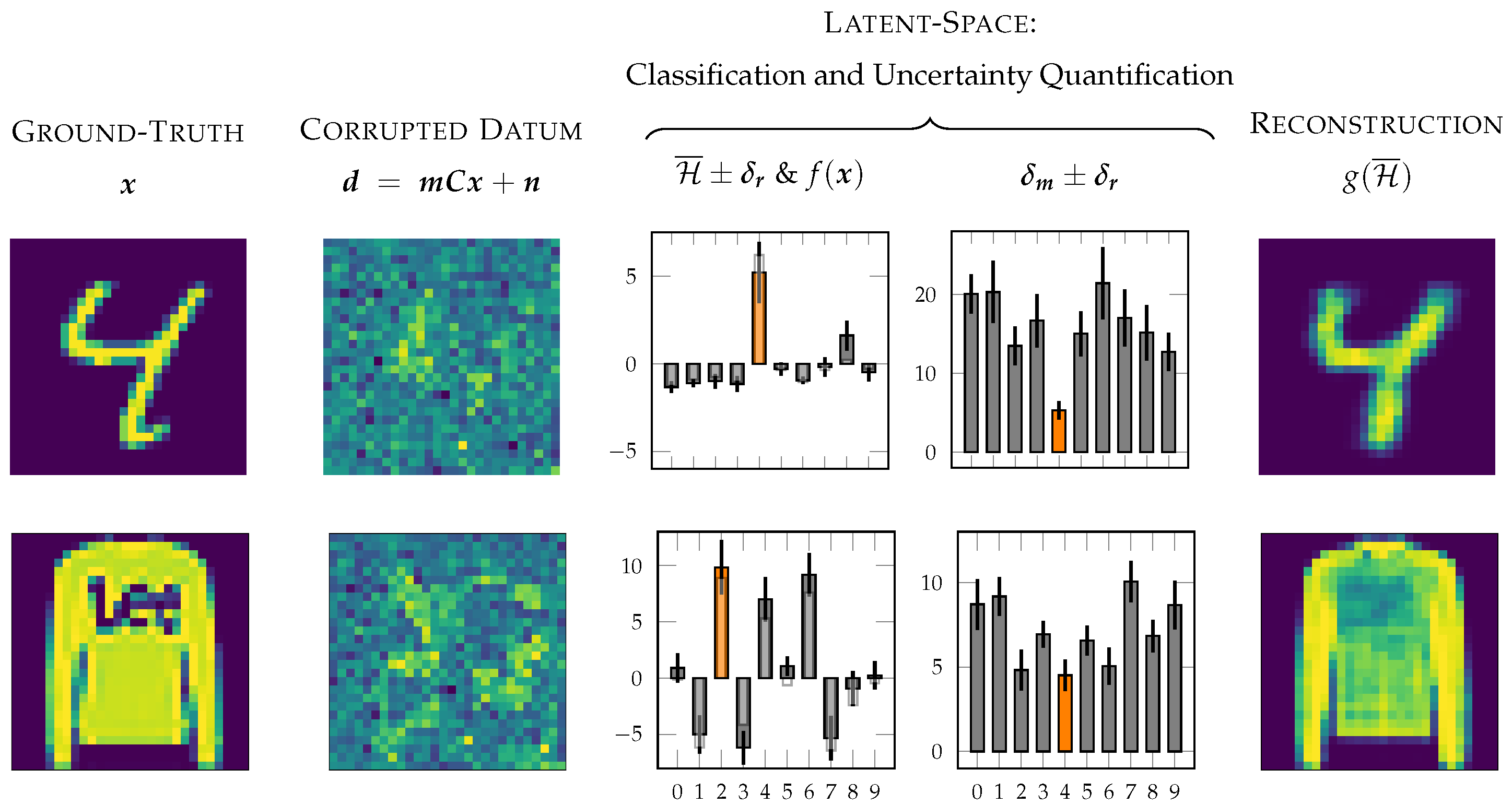
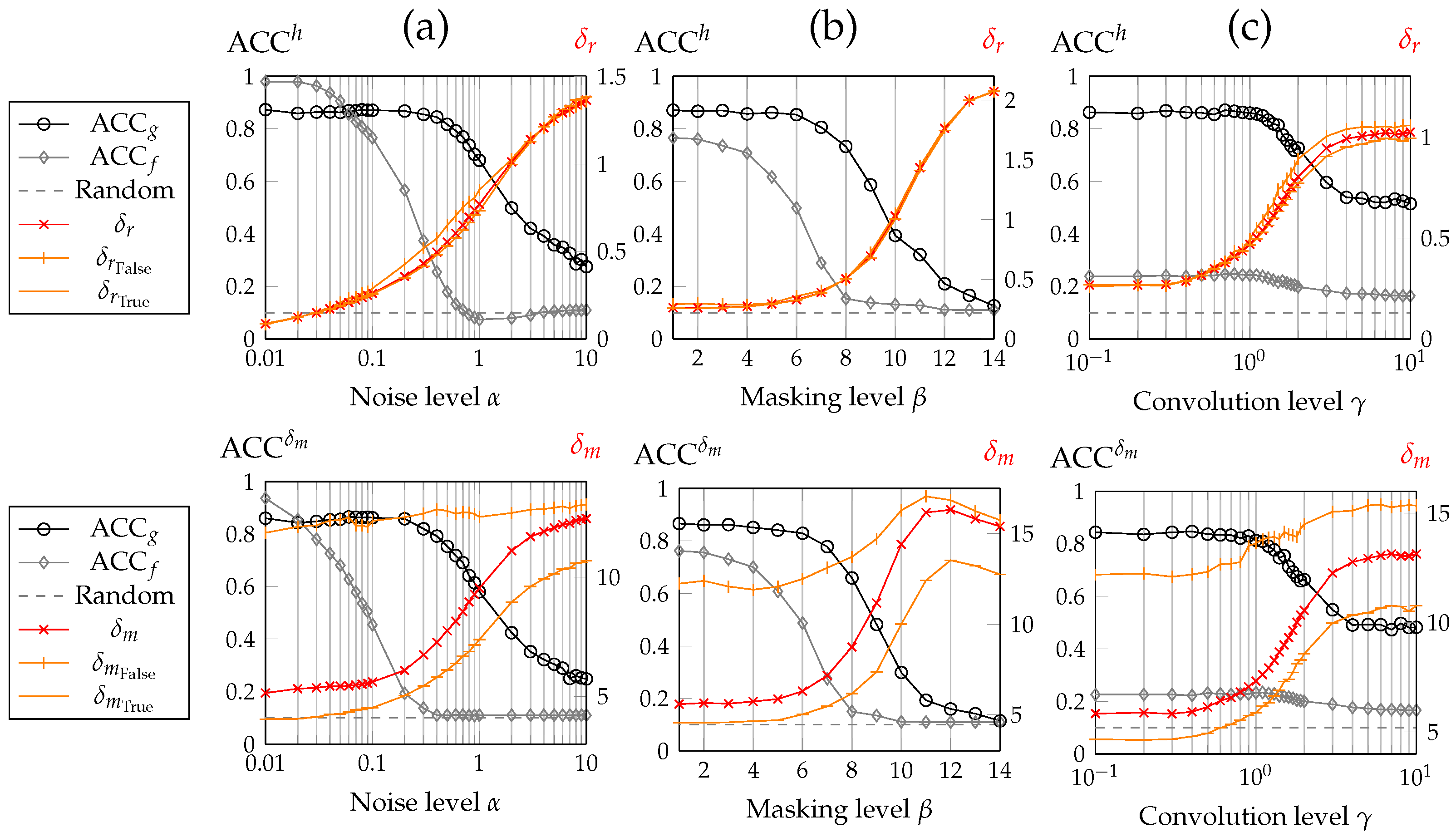
• The reconstruction uncertainty ${\mathit{\delta }}_{r_{\mathrm{True}}}$ of correct classifications is approximately equivalent to the ${\mathit{\delta }}_{r_{\mathrm{False}}}$ of wrong classifications. This behavior indicates that the correctness of the classification does not influence the reconstruction uncertainty ${\mathit{\delta }}_r$, showing evidence that ${\mathit{\delta }}_r$ is independent of the model uncertainty ${\mathit{\delta }}_m$.
• As opposed to ${\mathit{\delta }}_r$, the model uncertainty ${\mathit{\delta }}_m$ strongly depends on the correct/wrong classification of the corrupted datum: ${\mathit{\delta }}_m$ is significantly and consistently higher for false classifications than for true classifications. This characteristic sets the basis for a statistical “lie detector” (see Section 3.2) of classification. Fields of application could be the validation of neural networks in, e.g., medical imaging and other safety-critical applications.
• Classifying corrupted data through the decoder (see ${\mathrm{ACC}}_g$ in Figure 3) (rather than the encoder (see ${\mathrm{ACC}}_f$)), with a suitable channel model considering the corruption, significantly improved the model’s accuracy without the necessity of retraining the autoencoder. Especially for high levels of all corruption types, the accuracy of the model notably improved. Corruption by convolution had catastrophic consequences for classifying data in a straightforward manner through the encoder f, while this type of corruption seemed to only have a minor impact on our method.
• Both uncertainties ${\mathit{\delta }}_r$ and ${\mathit{\delta }}_m$ rose with increasing levels of corruption.

3.2. Detection of False Classifications

Finally, in experiment (4) (see Figure 5), we validated the model uncertainty of our method by introducing the Uncertainty-based Receiver Operating Characteristics (U-ROC) curve of detecting false classifications with the M-distance. We evaluated the binary classification task of the two classes “The neural network correctly classifies a corrupted datum” (Positive Class) and “The neural network falsely classifies a corrupted datum” (Negative Class). Based on the model uncertainty of our method, we aimed to predict the two classes without further knowledge, providing the initially proposed “lie detector”. The U-ROC curve was built from the True Positive Rate and the False Positive Rate. We compared our U-ROC curve with the U-ROC curve of the MC-dropout method [10] and with the U-ROC curve of EDL [11], feeding all methods with the identical input of a datum corrupted by noise at $\alpha =[0.1,0.5,1.0]$. We made the following conclusions from experiment (4), Figure 5:

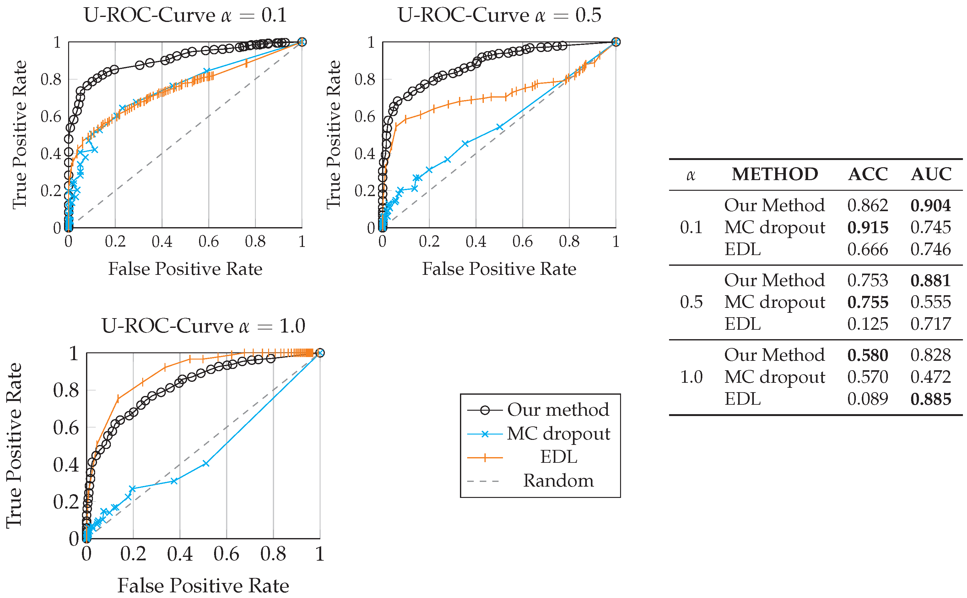
• Our method seemed to outperform MC-dropout and EDL to detect false classifications given the same data samples at the input for $\alpha =0.1$ and $\alpha =0.5$. One reason for this might be that the M-distance serves as a reliable out-of-distribution detector, exploiting the inherent latent space structure of uncorrupted data as a reference, as opposed to MC-dropout and EDL. For $\alpha =1.0$, both EDL and our method outperformed MC-dropout, while the Area Under the Curve (AUC) of EDL was largest. Here, it should be noted that EDL cannot classify the corrupted data at this noise level (accuracy: $8.9\%$), resulting in only few samples to test the cases of True Positives and False Positives.
• All three methods provided reliable results for detecting false classifications for low noise levels. The model uncertainty ${\mathit{\delta }}_m$ truly reflects the confidence of the classification, i.e., a high value of ${\mathit{\delta }}_m$ correlates empirically with a higher probability of false classification.
• The U-ROC curve combined with the accuracy indicates that EDL seemed to overestimate uncertainties, leading to a very robust U-ROC curve for high noise levels, but simultaneously leading to a severe drop in the accuracy in the presence of data corruption. We observed comparable results on F-MNIST data.

4. Requirements and Summary

Our proposed methodology to classify a corrupted datum $\mathit{d}$ including uncertainty quantification requires the following inputs in addition to $\mathit{d}$:

• $\mathit{m},\mathit{C}$: Without loss of generality, here, we assumed corruption by masking and convolution represented by $\mathit{m}$ and $\mathit{C}$ in the AWGN channel model, as depicted in Equation (2). Here, $\mathit{C}$ can in real-world applications often be derived from the image processing system in use. Algorithms to detect possibly occluding objects (represented by masking $\mathit{m}$) were given by, e.g., [20].
• ${\Sigma }_{\mathit{n}}$: Noise covariance matrix. AWGN with $n\sim \mathcal{N}(0,{\Sigma }_n)$ and applied additively to the data $\mathit{d}$. Among others, the methodology published by [21] enables the derivation of ${\Sigma }_{\mathit{n}}$ given noisy data $\mathit{d}$.
• ${\Sigma }_{\mathit{h}}$: Sampling covariance matrix of all (uncorrupted) latent space activations processed by the encoding function f. We used the assumption that an autoencoder can represent an inherent, lower-dimensional structure of the data in its latent space and assumed this sub-dimensional structure to sufficiently follow a multivariate Gaussian probability distribution.

In summary, our approach was able to classify heavily corrupted data with parametric classifiers. The method does not require corrupted data for training. As we built our procedure on a probabilistic architecture, we quantified the classification and the model uncertainties, allowing for a reliable detection of false classifications. We see our method as a highly flexible and robust framework that can be applied to any generative neural network to improve performance on corrupted data significantly. If the generative neural network comes with a supervised encoded space, it can classify the data directly. We showed that the M-distance can independently be used to classify data. The limitations of our method include that the corruption type needs to be modeled, as well as there is a higher computational cost than MC-dropout and EDL (mainly due to the approximation of the posterior probability distribution; Step 4 in Section 2.1).

References

- Le, L.; Patterson, A.; White, M. Supervised autoencoders: Improving generalization performance with unsupervised regularizers. In NIPS’18: Proceedings of the 32nd International Conference on Neural Information Processing Systems, Montréal, Canada, 3–8 December 2018; Curran Associates, Inc.: Red Hook, NY, USA, 2018; pp. 107–117. [Google Scholar]
- Knollmüller, J.; Enßlin, T. Metric Gaussian Variational Inference. arXiv 2020, arXiv:1901.11033. [Google Scholar]
- Lee, K.; Lee, K.; Lee, H.; Shin, J. A Simple Unified Framework for Detecting out-of-Distribution Samples and Adversarial Attacks. In NIPS’18: Proceedings of the 32nd International Conference on Neural Information Processing Systems, Montréal, Canada, 3–8 December 2018; Curran Associates, Inc.: Red Hook, NY, USA, 2018; pp. 7167–7177. [Google Scholar]
- Böhm, V.; Lanusse, F.; Seljak, U. Uncertainty Quantification with Generative Models. arXiv 2019, arXiv:1910.10046. [Google Scholar]
- Böhm, V.; Seljak, U. Probabilistic Auto-Encoder. arXiv 2020, arXiv:2006.05479. [Google Scholar]
- Adler, J.; Öktem, O. Deep Bayesian Inversion. arXiv 2018, arXiv:1811.05910. [Google Scholar]
- Seljak, U.; Yu, B. Posterior Inference Unchained with EL_2O. arXiv 2019, arXiv:1901.04454. [Google Scholar]
- Wu, G.; Domke, J.; Sanner, S. Conditional Inference in Pre-trained Variational Autoencoders via Cross-coding. arXiv 2018, arXiv:1805.07785. [Google Scholar]
- Neal, R.M. Bayesian Learning for Neural Networks; Springer: Berlin/Heidelberg, Germany, 1995. [Google Scholar]
- Gal, Y.; Ghahramani, Z. Dropout as a Bayesian Approximation: Representing Model Uncertainty in Deep Learning. In Proceedings of the 33rd International Conference on Machine Learning, New York, NY, USA, 19–24 June 2016; Volume 48, pp. 1050–1059. [Google Scholar]
- Sensoy, M.; Kaplan, L.; Kandemir, M. Evidential Deep Learning to Quantify Classification Uncertainty. In NIPS’18: Proceedings of the 32nd International Conference on Neural Information Processing Systems, Montréal, Canada, 3–8 December 2018; Curran Associates, Inc.: Red Hook, NY, USA, 2018; pp. 3183–3193. [Google Scholar]
- Vincent, P.; Larochelle, H.; Bengio, Y.; Manzagol, P.A. Extracting and composing robust features with denoising autoencoders. In Proceedings of the 25th International Conference on Machine Learning, Helsinki, Finland, 5–9 July 2008; pp. 1096–1103. [Google Scholar]
- Kingma, D.P.; Ba, J. Adam: A Method for Stochastic Optimization. In Proceedings of the 3rd International Conference on Learning Representations, ICLR 2015, San Diego, CA, USA, 7–9 May 2015. [Google Scholar]
- Kingma, D.P.; Welling, M. Auto-Encoding Variational Bayes. In Proceedings of the 2nd International Conference on Learning Representations, ICLR 2014, Banff, AB, Canada, 14–16 April 2014. [Google Scholar]
- Kucukelbir, A.; Tran, D.; Ranganath, R.; Gelman, A.; Blei, D.M. Automatic Differentiation Variational Inference. J. Mach. Learn. Res. 2017, 18, 430–474. [Google Scholar]
- LeCun, Y. The MNIST database of Handwritten Digits. 1998. Available online: http://yann.lecun.com/exdb/mnist/ (accessed on 6 June 2020).
- Xiao, H.; Rasul, K.; Vollgraf, R. Fashion-MNIST: A Novel Image Dataset for Benchmarking Machine Learning Algorithms. arXiv 2017, arXiv:1708.07747. [Google Scholar]
- Klambauer, G.; Unterthiner, T.; Mayr, A.; Hochreiter, S. Self-Normalizing Neural Networks. In NIPS’17: Proceedings of the 31st International Conference on Neural Information Processing Systems, Long Beach, CA, USA, 4–9 December 2017; Curran Associates, Inc.: Red Hook, NY, USA, 2017; pp. 972–981. [Google Scholar]
- Selig, M.; Bell, M.R.; Junklewitz, H.; Oppermann, N.; Reinecke, M.; Greiner, M.; Pachajoa, C.; Enßlin, T.A. NIFTY–Numerical Information Field Theory-A versatile PYTHON library for signal inference. Astron. Astrophys. 2013, 554, A26. [Google Scholar] [CrossRef]
- Li, B.; Hu, W.; Wu, T.; Zhu, S.C. Modeling occlusion by discriminative and-or structures. In Proceedings of the IEEE International Conference on Computer Vision, Sydney, NSW, Australia, 1–8 December 2013; pp. 2560–2567. [Google Scholar]
- Liu, X.; Tanaka, M.; Okutomi, M. Noise level estimation using weak textured patches of a single noisy image. In Proceedings of the 2012 19th IEEE International Conference on Image Processing, Orlando, FL, USA, 30 September–3 October 2012; pp. 665–668. [Google Scholar]
Publisher’s Note: MDPI stays neutral with regard to jurisdictional claims in published maps and institutional affiliations. |
© 2022 by the authors. Licensee MDPI, Basel, Switzerland. This article is an open access article distributed under the terms and conditions of the Creative Commons Attribution (CC BY) license (https://creativecommons.org/licenses/by/4.0/).
Share and Cite
Joppich, P.; Dorn, S.; De Candido, O.; Knollmüller, J.; Utschick, W. Classification and Uncertainty Quantification of Corrupted Data Using Supervised Autoencoders. Phys. Sci. Forum 2022, 5, 12. https://doi.org/10.3390/psf2022005012
Joppich P, Dorn S, De Candido O, Knollmüller J, Utschick W. Classification and Uncertainty Quantification of Corrupted Data Using Supervised Autoencoders. Physical Sciences Forum. 2022; 5(1):12. https://doi.org/10.3390/psf2022005012
Chicago/Turabian StyleJoppich, Philipp, Sebastian Dorn, Oliver De Candido, Jakob Knollmüller, and Wolfgang Utschick. 2022. "Classification and Uncertainty Quantification of Corrupted Data Using Supervised Autoencoders" Physical Sciences Forum 5, no. 1: 12. https://doi.org/10.3390/psf2022005012
APA StyleJoppich, P., Dorn, S., De Candido, O., Knollmüller, J., & Utschick, W. (2022). Classification and Uncertainty Quantification of Corrupted Data Using Supervised Autoencoders. Physical Sciences Forum, 5(1), 12. https://doi.org/10.3390/psf2022005012