Survey Optimization via the Haphazard Intentional Sampling Method ^†

Abstract

In previously published articles, our research group has developed the Haphazard Intentional Sampling method and compared it to the Rerandomization method proposed by K.Morgan and D.Rubin. In this article, we compare both methods to the pure randomization method used for the Epicovid19 survey, conducted to estimate SARS-CoV-2 prevalence in 133 Brazilian Municipalities. We show that Haphazard intentional sampling can either substantially reduce operating costs to achieve the same estimation errors or, the other way around, substantially improve estimation precision using the same sample sizes.

1. Introduction

Traditional sampling with face-to-face interviews usually demands large staff and infrastructure and expensive field operations to cover a representative group of the population of interest. Even then, pure (or stratified) randomized experiments do not guarantee efficient control over specific sets of covariates, and there may be large divergences between sample and population statistics. To address this problem, Lauretto et al. [1, 2] and Fossaluza et al. [3] developed the Haphazard Intentional Sampling method, an approach that combines intentional sampling, using methods of numerical optimization for an appropriate objective function, with random disturbances ensuring good decoupling properties. The word haphazard was used by Dennis Lindley to distinguish the decoupling effect from the tool used to obtain the desired decoupling, namely, randomization; for further details, see [1,3,4]. For a fixed sample size, this technique aims at diminishing the distance between sample and population regarding specific covariates of interest or, the other way around, minimizing the sample size needed to achieve good enough expected agreement between sample and population regarding specific covariates of interest. The Mahalanobis distance is the natural choice for the statistical model at hand, but other $L_p$ distances, or convex combinations thereof, will be used as approximations useful for numerical computation, as explained in the following sections. This method can be applied in several contexts, such as allocations of treatment and control groups in medical trials [2] or in statistical sampling problems [5]. In this method, a weight factor, $\lambda$, adjusts the weight of the random perturbation relative to the deterministic objective function of the optimization problem. In practical problems, the weight factor $\lambda$ can be calibrated in such a way that, on the one hand, it is small enough to generate only slightly sub-optimal solutions and, on the other hand, it is large enough to break potential confounding effects that could introduce spurious statistical biases in the study.

In this paper, the performance of the Haphazard intentional sampling method is compared to pure random sampling and to the Rerandomization methods proposed by Morgan and Rubin [6]. As a benchmark, we use an artificial sampling problem concerning inferences about the prevalence of Sars-CoV-2, using covariates from public data sets generated by the 2010 Census of the Brazilian Institute of Geography and Statistics (IBGE). Pending analyses of this benchmark study, real epidemiological applications shall be developed in the near future. Sampling procedures of the three aforementioned methods were repeatedly applied to the benchmark problem, in order to obtain performance statistics regarding how well generated samples represent the population.

2. Haphazard Intentional Sampling Method

In this section, we present the formulation of the Haphazard intentional sampling method presented by Lauretto et al. [1,2]. Let $\mathbf{X}$ denote a matrix in ${\mathbb{R}}^{n\times d}$, where n is the number of candidate sampling units and d is the number of covariates of interest. An allocation consists of assigning to each unit a group chosen from a set of possible groups, $\mathcal{G}=\{0,1,2,...g\}$. We denote by $\mathbf{w}$ an allocation vector in ${\mathcal{G}}^n$, assigning each unit to a group. For simplicity, we assume only two groups, that is, $\mathcal{G}=\{0,1\}$, the control and treatment groups, or the unsampled and sampled units. We also assume that the number of units assigned to each group is previously defined. That is, integers $n_1$ and $n_0$ exist such that $n_1+n_0=n$, $\mathbf{1}{\mathbf{w}}^t=n_1$ and $\mathbf{1}{(\mathbf{1}-\mathbf{w})}^t=n_0$. $\mathbf{1}$ denotes a vector of ones with the proper size; therefore, the scalar product $\mathbf{1}{\mathbf{w}}^t$ is the sum of the scalar components of $\mathbf{w}$. The goal of the allocation problem is to generate an allocation, $\mathbf{w}$, that, with high probability, approximately minimizes the imbalance between groups with respect to a loss function, $L(\mathbf{w},\mathbf{X})$.

The Mahalanobis distance is the metric of choice for statistical models based on the multivariate normal distribution; for further details, see Stern [7] (Section 6.2). The Mahalanobis distance between the covariates of interest in each group is defined as follows. Let $\mathbf{A}$ be an arbitrary matrix in ${\mathbb{R}}^{n\times m}$. Furthermore, define ${\mathbf{A}}^{*}:=\mathbf{A}\mathbf{L}$, where $\mathbf{L}$ is the lower triangular Cholesky factor [8] of the inverse of covariance matrix of $\mathbf{A}$; that is, $\mathrm{Cov}{\left(\mathbf{A}\right)}^{-1}=\mathbf{L}{\mathbf{L}}^t$.

For an allocation $\mathbf{w}$, let ${\overline{{\mathbf{A}}^{*}}}^1$ and ${\overline{{\mathbf{A}}^{*}}}^0$ denote the averages of each column of ${\mathbf{A}}^{*}$ over units allocated to, respectively, groups 1 and 0 according to the row vector $\mathbf{w}$:

$${\overline{{\mathbf{A}}^{*}}}^1:=(1/n_1)\mathbf{w}{\mathbf{A}}^{*}\mathrm{and}{\overline{{\mathbf{A}}^{*}}}^0:=(1/n_0)(\mathbf{1}-\mathbf{w}){\mathbf{A}}^{*}.$$

(1)

The Mahalanobis distance between the average of the column values of $\mathbf{A}$ in each group specified by $\mathbf{w}$ is defined as:

$$M(\mathbf{w},\mathbf{A}):=m^{-1}{\parallel {\overline{{\mathbf{A}}^{*}}}^1-{\overline{{\mathbf{A}}^{*}}}^0\parallel }_2,$$

(2)

where m denotes the number of columns of A.

2.1. Pure Intentional Sampling Formulation

Under the Mahalanobis loss function, a pure intentional sampling procedure consists of generating an allocation $\mathbf{w}$ that minimizes the following optimization problem:

$$\begin{array}{cc}\mathrm{minimize}\hfill & {\displaystyle M(\mathbf{w},\mathbf{X})}\hfill \\ \mathrm{subject\; to}\hfill & {\displaystyle \mathbf{1}{\mathbf{w}}^t=n_1}\hfill \\ \hfill & {\displaystyle \mathbf{1}{(\mathbf{1}-\mathbf{w})}^t=n_0}\hfill \\ \hfill & {\displaystyle \mathbf{w}\in {\{0,1\}}^n}\hfill \end{array}$$

(3)

The formulation presented in Equation (3) is a Mixed-Integer Quadratic Programming Problem (MIQP) [9], that can be computationally very expensive. The hybrid loss function, $H(\mathbf{w},\mathbf{A})$, is a surrogate function for $M(\mathbf{w},\mathbf{A})$ built using a linear combination of $L_1$ and $L_{\infty }$ norms; see Ward and Wendell [10]:

$$H(\mathbf{w},\mathbf{A}):=m^{-1}\left(\parallel {\overline{{\mathbf{A}}^{*}}}^1-{\overline{{\mathbf{A}}^{*}}}^0{\parallel }_1+\sqrt{m}{\parallel {\overline{{\mathbf{A}}^{*}}}^1-{\overline{{\mathbf{A}}^{*}}}^0\parallel }_{\infty }\right)$$

(4)

The minimization of $H(\mathbf{w},\mathbf{A})$ yields the Mixed-Integer Linear Programming Problem (MILP) defined in the next equation, which is computationally much less expensive than the MIQP problem (3); see Murtagh [11] and Wolsey and Nemhauser [9].

$$\begin{array}{cc}\mathrm{minimize}\hfill & {\displaystyle H(\mathbf{w},\mathbf{X})}\hfill \\ \mathrm{subject\; to}\hfill & {\displaystyle \mathbf{1}{\mathbf{w}}^t=n_1}\hfill \\ \hfill & {\displaystyle \mathbf{1}{(\mathbf{1}-\mathbf{w})}^t=n_0}\hfill \\ \hfill & {\displaystyle \mathbf{w}\in {\{0,1\}}^n}\hfill \end{array}$$

(5)

Statistical inference based on pure intentional sampling is vulnerable to malicious manipulation, unconscious biases, and many other confounding effects. In the Frequentist School of statistics, the use of intentional allocation is anathema, whereas in the Bayesian School, it has been the subject of long-standing debates. The solution presented in this paper is a compromise aiming to achieve the effective performance of intentional sampling but using moderate randomization to avoid systematic confounding effects. Lauretto et al. [1] and Fossaluza et al. [3] give a thorough discussion of the motivation and history of the ideas leading to the Haphazard intentional sampling method.

2.2. Haphazard Formulation

The Haphazard intentional sampling method consists of extending the pure intentional sampling method, formulated in Equation (5), as a MILP optimization problem, with the introduction of a noisy component. Let $\mathbf{Z}$ be an artificially generated random matrix in ${\mathbb{R}}^{n\times k}$, with elements that are independent and identically distributed according to the standard normal distribution. For a given tuning parameter, $\lambda \in [0,1]$, the Haphazard method, aims to solve the following optimization problem:

$$\begin{array}{cc}\mathrm{minimize}\hfill & {\displaystyle (1-\lambda )H(\mathbf{w},\mathbf{X})+\lambda H(\mathbf{w},\mathbf{Z})}\hfill \\ \mathrm{subject\; to}\hfill & {\displaystyle \mathbf{1}{\mathbf{w}}^t=n_1}\hfill \\ \hfill & {\displaystyle \mathbf{1}{(\mathbf{1}-\mathbf{w})}^t=n_0}\hfill \\ \hfill & {\displaystyle \mathbf{w}\in {\{0,1\}}^n}\hfill \end{array}$$

(6)

The parameter $\lambda$ controls the amount of perturbation that is added to the surrogate loss function, $H(\mathbf{w},\mathbf{X})$. If $\lambda =0$, then ${\mathbf{w}}^{*}$ is the deterministic optimal solution for $H(\mathbf{w},\mathbf{X})$, corresponding to the pure intentional sampling. If $\lambda =1$, then ${\mathbf{w}}^{*}$ is the optimal solution for the artificial random loss, $H(\mathbf{w},\mathbf{Z})$, corresponding to a completely random allocation. By choosing an intermediate value of $\lambda$ (as discussed in Section 3.2), one can obtain ${\mathbf{w}}^{*}$ to be a partially randomized allocation such that, with a high probability, $H({\mathbf{w}}^{*},\mathbf{X})$ is close to the minimum loss.

3. Case Study

The artificial data set used for the simulations carried in this study are inspired by Epicovid19 [12], a survey conducted by the Brazilian Institute of Public Opinion and Statistics (IBOPE) and the Federal University of Pelotas (UFPel) to estimate SARS-CoV-2 infection prevalence in 133 Brazilian municipalities. Our study is supplemented by data from the 2010 Brazilian census conducted by IBGE, giving socio-economic information by census sector. Sectors are the minimal units by which census information is made publicly available. Typically, each sector has around 200 households. Furthermore, households in a sector form a contiguous geographic area with approximately homogeneous characteristics.

The first step of the sampling procedure of Epicovid19 study consisted of randomly selecting a subset of census sectors of each surveyed municipality. As a second step, at each of the selected sectors, a subset of households was randomly selected for a detailed interview concerning socio-economic characteristics and SARS-CoV-2 antibody testing. Our benchmark problem is based on the original Epicovid19 study, where we evaluate the impact of alternative census sector sampling procedures on the estimation of the response variable, namely, SARS-CoV-2 prevalence. In order to simulate outcomes for alternative sector selections, we used an auxiliary regression model for this response variable, as explained in the sequel.

3.1. Auxiliary Regression Model for SARS-CoV-2 Prevalence

The auxiliary regression model for SARS-CoV-2 prevalence had the Epicovid19 estimated infection rates adjusted for the spread of the pandemic in subsequent months and corrected for underreporting due to lack of intensive testing in Brazil. As explanatory variables, this auxiliary model used 15 socio-demographic covariates, including income, ethnicity, age, sanitation condition, etc. The parameters of this auxiliary regression model were estimated using standard regression packages available at the R statistical environment. Since the response variable is simulated by this auxiliary regression model, its covariates and their weight coefficients in the regression can be taken as a valid representativity target, that is, the Haphazard and Rerandomization methods will try to make sector selections that resemble the population characteristics corresponding to these 15 covariates.

The auxiliary model was a logit link regression, specified by selecting three of the most relevant predictive variables, namely, average income, population percentage with zero income, and percentage of households with two or more bathrooms (a standard indirect measure of wealth used by IBGE):

$$ln(p_i/(1-p_i))={\eta }_i=\widehat{{\beta }_0}+\widehat{{\beta }_1}{x}_{i,1}+\widehat{{\beta }_2}{x}_{i,2}+\widehat{{\beta }_3}{x}_{i,3}+{ϵ}_i$$

(7)

$$p_i=\frac{e^{{\eta }_i}}{(1+e^{{\eta }_i})}$$

(8)

$p_i$: simulated SARS-CoV-2 prevalence in sector i;

$x_{i,1}$: income in census sector i;

$x_{i,2}$: zero income population percentage in census sector i;

$x_{i,3}$: percentage of households with two or more bathrooms in census sector i.

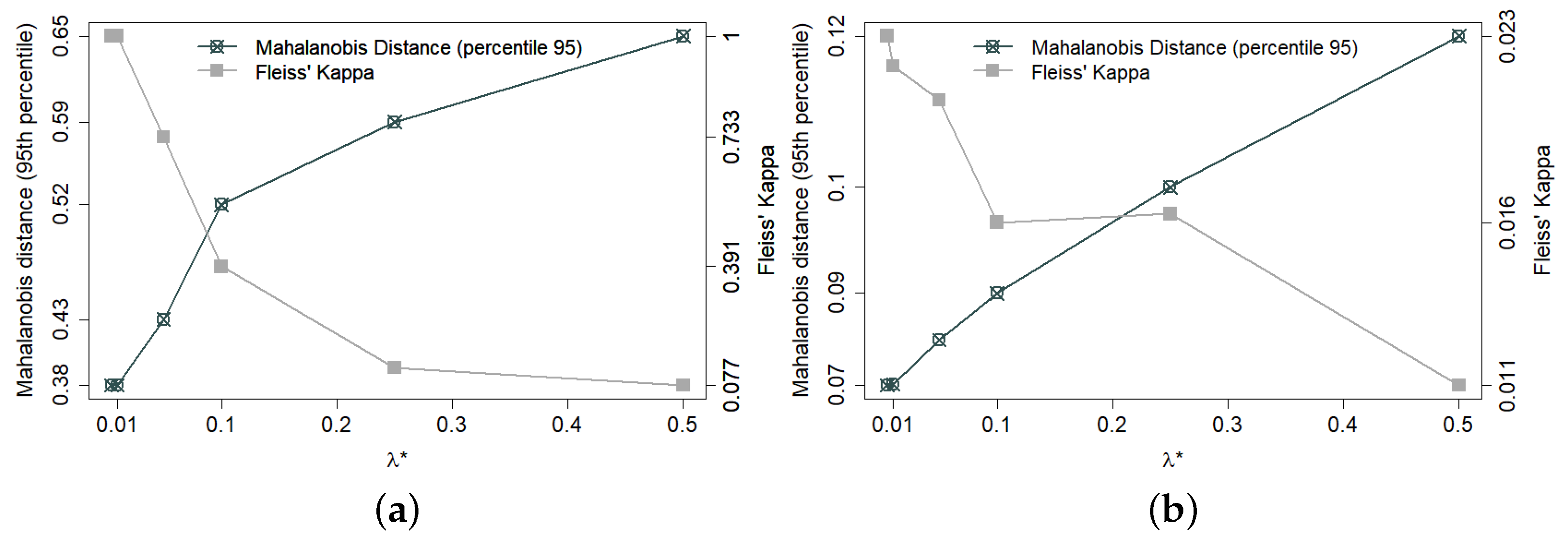
3.2. Balance and Decoupling Trade-Off in the Haphazard Method

The Haphazard intentional sampling method is not exclusively concerned with choosing maximally representative samples. Equally important is to prevent estimation biases induced by spurious confounding effects. This is exactly the role of the decoupling effects engendered by standard randomization procedures. We need a quantitative measure to assess how effectively the noise introduced in the method, with weight $\lambda$, is performing this task. A proxy measure of this sort can be constructed using Fleiss’ Kappa coefficient, conceived to measure the degree of agreement between nominal scales assigned by multiple raters, see Fleiss [13]. In our context, it is used as follows.

For r repetitions of a sampling procedure, let $r_{i,j}$ denote the number of times element $i\in \{1,2,\cdots ,N\}$ is allocated to group $j\in \{0,1\}$. Let ${\overline{P}}_o$ denote the observed average proportion of concordance among all allocation pairs. Let ${\overline{P}}_e$ denote the expected agreement that would be obtained by chance, conditional on the proportion of assignments that were observed in each group j.

$${\overline{P}}_o=\frac{1}{Nr(r-1)}\sum _{i=1}^N\sum _{j=0}^1{r}_{i,j}(r_{i,j}-1){\overline{P}}_e=\sum _{j=0}^1\frac{{\left({\sum }_{i=1}^N{r}_{i,j}\right)}^2}{{\left(Nr\right)}^2}$$

(9)

The Fleiss’ Kappa coefficient is obtained by the ratio of the difference between the observed and the expected random agreement, ${\overline{P}}_o-{\overline{P}}_e$, and the difference between total agreement and the agreement obtained by chance, $1-{\overline{P}}_e$:

$$\kappa =\frac{{\overline{P}}_o-{\overline{P}}_e}{1-{\overline{P}}_e}$$

(10)

The relation between decoupling and the degree of disturbance added is assessed empirically. The following transformation between parameters $\lambda$ and ${\lambda }^{*}$ is devised to equilibrate the weights given to the terms of Equation (6) corresponding to the covariates of interest and artificial noise, according to dimensions d (the number of columns of $\mathbf{X}$) and k (the number of columns of $\mathbf{Z}$).

$$\lambda ={\lambda }^{*}/\left[{\lambda }^{*}(1-k/d)+k/d\right],\mathrm{where}{\lambda }^{*}\in \{0.005,0.01,0.05,0.1,0.25,0.5\}.$$

(11)

The trade-off between balancing and decoupling also varies according to the characteristics of each municipality. Small municipalities have only a limited number of census sectors and, hence, also a limited set of near-optimal solutions. Therefore, for small municipalities, good decoupling requires a larger ${\lambda }^{*}$. Figure 1a shows, for the smallest of the 133 municipalities in the database (with 34 census sectors), the trade-off between balance and decoupling (Fleiss’ Kappa) as ${\lambda }^{*}$ varies in proper range. Figure 1b shows the same trade-off for a medium sized municipality. Since it has many more sectors (176), it is a lot easier to find well-balanced solutions and, hence, good decoupling is a lot easier to achieve.

Larger municipalities engender larger optimization problems (for the number of binary decision variables equals the number of census sectors) that, in turn, usually require more CPU time for the MILP solver.

Table 1. Parameters ${\lambda }^{*}$ and maximum CPU time for MILP solver by number of sectors.

Sectors	${\mathit{\lambda }}^{*}$	Time (s)
<50	0.1	5
50–4000	0.01	30
>4000	0.001	120

displays empirically calibrated parameters ${\lambda }^{*}$ and maximum CPU times under the hardware configuration described in Section 3.3.

3.3. Benchmark Experiments and Computational Setups

Our performance experiments used a subset of 10 municipalities of the 133 in the original Epicovid19 study, covering a wide range of population size and characteristics. Following the original Epicovid19 protocol, a sample of 25 census sectors was selected at each municipality. The sampling procedure for selecting these 25 sectors was repeated 300 times, using each of the three methods under comparison, namely, Haphazard method, Rerandomization, and pure randomization.

Numerical optimization and statistical computing tasks were implemented using the R v.3.6.1. environment [14] and the Gurobi v.9.0.1 optimization solvers [15]. The computer used to run these routines had an AMD RYZEN 1920X processor (3.5 GHz, 12 cores, 24 threads), ASROCK x399 motherboard, 64 GB DDR4 RAM, and Linux Ubuntu 18.04.5 LTS operating system. There is nothing particular about hardware configuration, with performance being roughly proportional to general computing power.

4. Experimental Results

In this section, we present the comparative results for the Haphazard, Rerandomization, and simple randomization methods, considering the metrics discussed in the sequel.

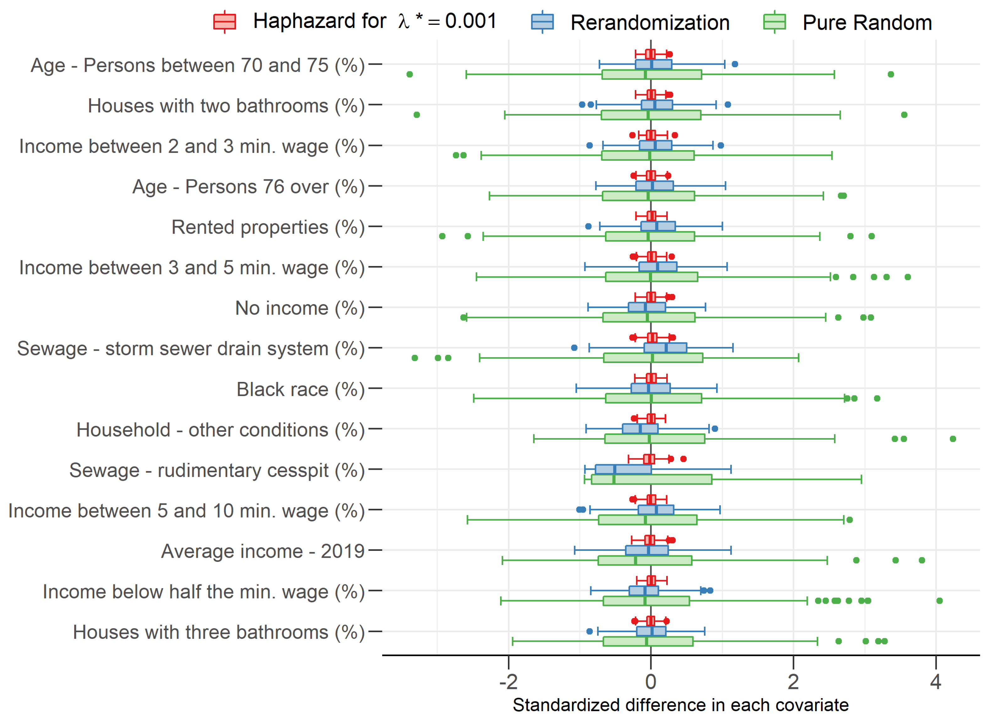
4.1. Group Unbalance among Covariates

We compute the standardized difference between group means for each covariate, based on 300 simulated allocations per method. Specifically, we compute the empirical distribution of the statistics $({\overline{\mathbf{X}}}_{,j}^1-{\overline{\mathbf{X}}}_{,j}^0)/s_j$, where ${\overline{\mathbf{X}}}_{,j}^1$ and ${\overline{\mathbf{X}}}_{,j}^0$ denote the averages of the j-th column of $\mathbf{X}$ over units allocated to, respectively, groups 1 and 0 (see Equation (1)); and $s_j$ is the reference scale given by the standard deviation of ${\overline{\mathbf{X}}}_{,j}^1-{\overline{\mathbf{X}}}_{,j}^0$ computed over 300 pure random allocations.

Figure 2 shows the distribution of standardized differences in each covariate (see Morgan and Rubin [16]) for São Paulo, the largest Brazilian municipality (18,182 sectors). It can be easily seen that differences are remarkably smaller for the haphazard allocations than for the rerandomization allocations, which, in turn, are remarkably smaller than for the pure randomization allocations. It is important to mention that this same pattern is verified in all other municipalities.

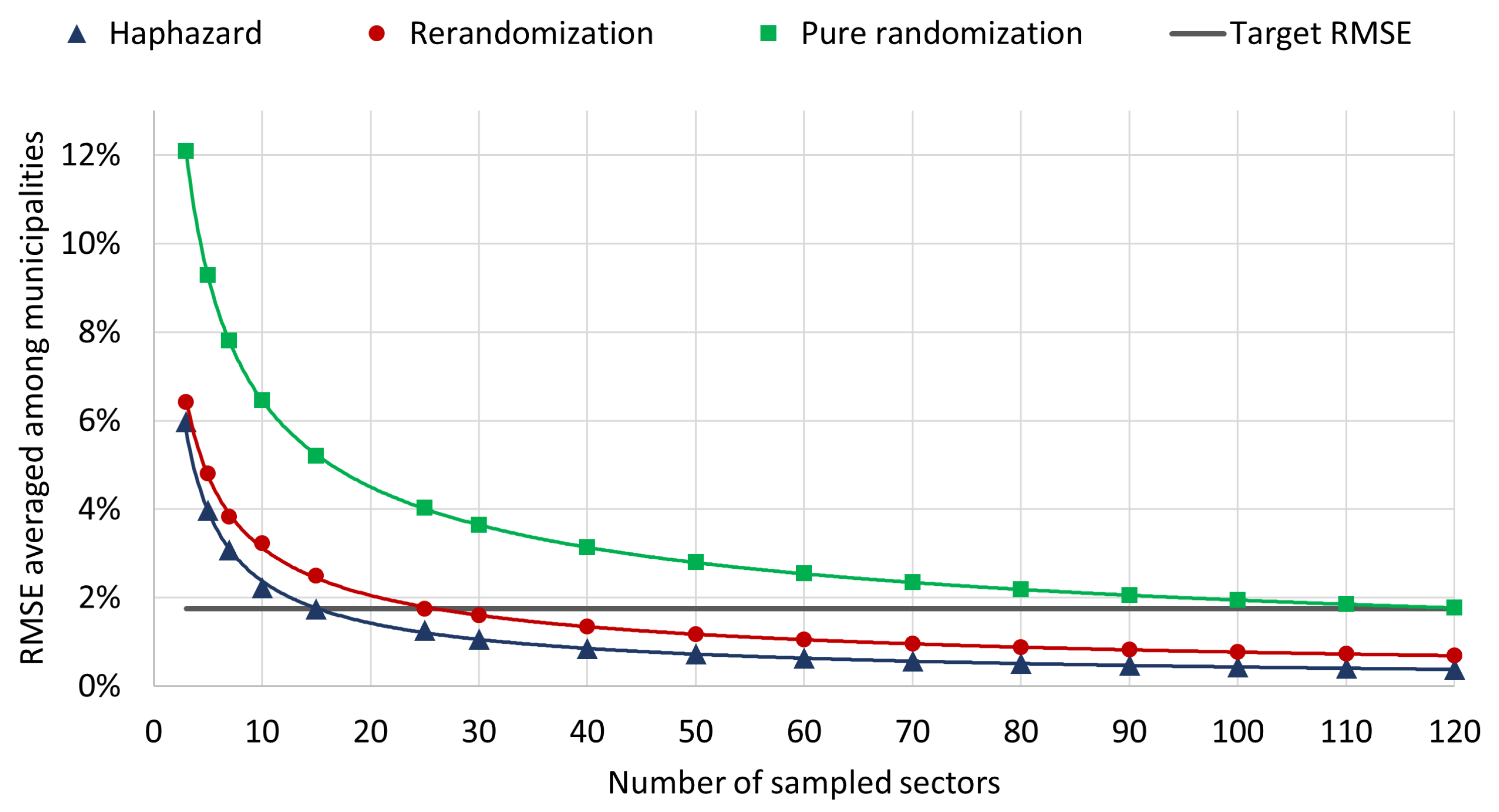
4.2. Root Mean Square Errors of Simulated Estimations

We now consider simulated scenarios where, once we have sampled the sectors in each municipality, we estimate the municipality’s SARS-CoV-2 prevalence based on observed prevalences on these sectors. Here, SARS-CoV-2 prevalence in each sector is simulated by the auxiliary regression model described in Section 3.1. To assess the estimation error yielded in each sampling method and to estimate variability, we compute, for each municipality, the root mean square error (RMSE) and the standard deviation of estimates, as follows:

$$RMSE\left(\widehat{\theta }\right)=\sqrt{\frac{1}{r}\sum _{a=1}^r{\left({\widehat{\theta }}_a-\theta \right)}^2}SD\left(\widehat{\theta }\right)=\sqrt{\frac{1}{r-1}\sum _{a=1}^r{\left({\widehat{\theta }}_a-E\left(\widehat{\theta }\right)\right)}^2},$$

(12)

where $r=300$ denotes the number of allocations, ${\widehat{\theta }}_a$ denotes the SARS-CoV-2 prevalence estimated from allocation a, $\theta$ denotes the SARS-CoV-2 prevalence considering all sectors of the municipality, and $E(\widehat{\theta })$ denotes the average of ${\widehat{\theta }}_a$ computed over r allocations.

Table 2. Root mean square error (RMSE) and standard deviation (SD); red: best result; black: worst.

City	Haphazard		Rerandomizaton		Pure Randomizaton
	RMSE	SD	RMSE	SD	RMSE	SD
São Paulo	1.6558%	1.6516%	2.4683%	2.3900%	4.9930%	4.9899%
Rorainópolis	0.8582%	0.7487%	1.5116%	1.4310%	3.0028%	3.0008%
Rio de Janeiro	1.3864%	1.3310%	1.9441%	1.9394%	4.6324%	4.6216%
Oiapoque	1.3887%	1.3835%	1.7651%	1.7509%	3.2107%	3.2107%
Marília	1.1624%	1.1603%	1.4787%	1.4737%	3.4950%	3.4919%
Iguatu	0.8329%	0.8196%	1.3029%	1.3025%	3.9094%	3.9003%
Cruzeiro do Sul	1.3873%	1.3489%	2.0482%	2.0457%	5.0029%	5.0003%
Corrente	0.7496%	0.7000%	1.0708%	1.0665%	2.8250%	2.8230%
Campos dos Goytacazes	0.9419%	0.9350%	1.8786%	1.8522%	4.4839%	4.4829%
Brasília	1.7978%	1.3434%	1.5739%	1.5299%	3.9608%	3.9539%

presents the $RMSE(\widehat{\theta })$ and $SD(\widehat{\theta })$ yielded by each sampling method for the 10 municipalities selected for this study. Both the Haphazard and the Rerandomization methods show RMSEs and SDs that are much smaller than the pure randomization method. Moreover, the Haphazard method outperforms the Rerandomization method, in the following sense: (a) the Haphazard method yields smaller RMSEs than the Rerandomization methods (in 9 out of 10 municipalities for this simulation); (b) moreover, the SDs are substantially smaller for the Haphazard method.

The RMSEs analyzed in the last paragraphs can be used to compute the sample size required to achieve a target precision in the statistical estimation of SARS-CoV-2 prevalence (as mentioned in Section 3, each sampling unit consists of a census sector containing around 200 households; the sample size refers to the number of sectors to be selected from each municipality). Figure 3 shows RMSEs as a function of sample size. If the sample size for each municipality is calibrated in order to achieve the target precision of the original Epicovid19 study (black horizontal line), using the Haphazard method implies an operating cost 40% lower than using the Rerandomization method and 80% lower than using pure randomization.

5. Final Remarks

Both Haphazard and Rerandomization are promising methods in generating samples that provide good estimates of the population parameters with potentially reduced sample sizes and consequent operating costs. Alternatively, if we keep the same sample sizes, the use of Haphazard or Rerandomization methods will substantially improve the precision of statistical estimation. The Rerandomization method is simple to implement. The Haphazard intentional method requires the use of numerical optimization software and the empirical calibration of auxiliary parameters. Nevertheless, from a computational point of view, as the dimension of the covariate space or the number of elements to be allocated increases, the Haphazard method will be exponentially more efficient. Finally, the theoretical framework of the Rerandomization method has been fully developed [6,16]. In further research, we intend to better develop the theoretical framework of the Haphazard intentional sampling method and continue to show its potential for applied statistics.

References

1. Lauretto, M.S.; Nakano, F.; Pereira, C.A.B.; Stern, J.M. Intentional Sampling by goal optimization with decoupling by stochastic perturbation. AIP Conf. Proc. 2012, 1490, 189–201. [Google Scholar]
2. Lauretto, M.S.; Stern, R.B.; Morgan, K.L.; Clark, M.H.; Stern, J.M. Haphazard intentional allocation an rerandomization to improve covariate balance in experiments. AIP Conf. Proc 2017, 1853, 050003. [Google Scholar]
3. Fossaluza, V.; Lauretto, M.S.; Pereira, C.A.B.; Stern, J.M. Combining Optimization and Randomization Approaches for the Design of Clinical Trials. In Interdisciplinary Bayesian Statistics; Springer: New York, NY, USA, 2015; pp. 173–184. [Google Scholar]
4. Stern, J.M. Decoupling, Sparsity, Randomization, and Objective Bayesian Inference. Cybern. Hum. Knowing 2008, 15, 49–68. [Google Scholar]
5. Lauretto, M.S.; Stern, R.B.; Ribeiro, C.O.; Stern, J.M. Haphazard Intentional Sampling Techniques in Network Design of Monitoring Stations. Proceedings 2019, 33, 12. [Google Scholar] [CrossRef] [Green Version]
6. Morgan, K.L.; Rubin, D.B. Rerandomization to improve covariate balance in experiments. Ann. Stat. 2012, 40, 1263–1282. [Google Scholar] [CrossRef]
7. Stern, J.M. Symmetry, Invariance and Ontology in Physics and Statistics. Symmetry 2011, 3, 611–635. [Google Scholar] [CrossRef]
8. Golub, G.H.; Van Loan, C.F. Matrix Computations; JHU Press: Baltimore, MD, USA, 2012. [Google Scholar]
9. Wolsey, L.A.; Nemhauser, G.L. Integer and Combinatorial Optimization; John Wiley & Sons: Hoboken, NJ, USA, 2014. [Google Scholar]
10. Ward, J.; Wendell, R. Technical Note-A New Norm for Measuring Distance Which Yields Linear Location Problems. Oper. Res. 1980, 28, 836–844. [Google Scholar] [CrossRef]
11. Murtagh, B.A. Advanced Linear Programming: Computation And Practice; McGraw-Hill International Book Co.: New York, NY, USA, 1981. [Google Scholar]
12. EPICOVID19. Available online: http://www.epicovid19brasil.org/?page_id=472 (accessed on 21 August 2020).
13. Fleiss, J.L. Measuring nominal scale agreement among many raters. Am. Psychol. Assoc. (APA) 1971, 76, 378–382. [Google Scholar] [CrossRef]
14. R Core Team. R: A Language and Environment for Statistical Computing; R Foundation for Statistical Computing: Vienna, Austria, 2020. [Google Scholar]
15. Gurobi Optimization Inc. Gurobi: Gurobi Optimizer 9.01 Interface; R Package Version 9.01; Gurobi Optimization Inc.: Beaverton, OR, USA, 2021. [Google Scholar]
16. Morgan, K.L.; Rubin, D.B. Rerandomization to Balance Tiers of Covariates. J. Am. Stat. Assoc. 2015, 110, 1412–1421. [Google Scholar] [CrossRef] [PubMed] [Green Version]
Figure 1. Trade-off between balance and decoupling in 300 allocations for two municipalities containing, respectively, 34 (panel a) and 176 (panel b) sectors. Sectors are the minimal units by which census information is made publicly available, each containing about 200 households. Balance between allocated and non-allocated sectors is expressed by the 95th percentile of Mahalanobis distance. Decoupling is expressed by Fleiss’ Kappa coefficient—notice the different range in each case (a,b).
Psf 03 00004 g001
Figure 2. Difference between groups 1 (sampled sectors) and 0 (not sampled sectors) with respect to average standardized covariate values for each type of allocation.
Psf 03 00004 g002
Figure 3. RMSE averaged among municipalities x number of sampled sectors.
Psf 03 00004 g003