A Weakly Informative Prior for Resonance Frequencies ^†

Abstract

We derive a weakly informative prior for a set of ordered resonance frequencies from Jaynes’ principle of maximum entropy. The prior facilitates model selection problems in which both the number and the values of the resonance frequencies are unknown. It encodes a weakly inductive bias, provides a reasonable density everywhere, is easily parametrizable, and is easy to sample. We hope that this prior can enable the use of robust evidence-based methods for a new class of problems, even in the presence of multiplets of arbitrary order.

1. Introduction

An important problem in the natural sciences is the accurate measurement of resonance frequencies. The problem can be formalized by the following probabilistic model:

$$p(D,\mathit{x}|I)=p(D\left|\mathit{x}\right)p\left(\mathit{x}\right|I)\equiv \mathcal{L}(\mathit{x}\left)\pi \right(\mathit{x}),$$

(1)

where D is the data, $\mathit{x}={\left\{x_k\right\}}_{k=1}^K$ are the K resonance frequencies of interest, and I is the prior information about $\mathit{x}$. As an example instance of (1), we refer to the vocal tract resonance (VTR) problem discussed in Section 5 for which D is audio recorded from the mouth of a speaker; $\mathit{x}$ are a set of K VTR frequencies, and the underlying model is a sinusoidal regression model. Any realistic problem will include additional model parameters $\mathit{\theta }$, but these have been silently ignored by formally integrating them out of (1), i.e., $p(D,\mathit{x}|I)=\int \mathrm{d}\mathit{\theta }p(D,\mathit{x},\mathit{\theta }\left|I\right)$.

In this paper, we assume that the likelihood $\mathcal{L}\left(\mathit{x}\right)\equiv p\left(D\right|\mathit{x})$ is given, and our task is to choose an uninformative prior $\pi \left(\mathit{x}\right)\equiv p\left(\mathit{x}\right|I)$ from limited prior information I. A conflict arises, however:

$$\begin{array}{c}\mathrm{The}\mathrm{uninformative}\mathrm{priors}\pi \mathrm{most}\mathrm{commonly}\mathrm{chosen}\mathrm{to}\mathrm{express}\mathrm{limited}\\ \mathrm{prior}\mathrm{information}I\mathrm{are},\mathrm{in}\mathrm{practice},\mathrm{often}\mathrm{precluded}\mathrm{by}\mathrm{that}\mathrm{same}I.\end{array}$$

(2)

The goal of this paper is to describe this conflict (2) and to show how it can be resolved by adopting a specific choice for $\pi$. This allows robust inference of the number of resonances K in the important case of such limited prior information I, which in turn enables accurate measurement of the resonance frequencies $\mathit{x}$ with standard methods such as nested sampling [1] or reversible jump MCMC [2].

2. Notation

The symbol $\pi$ is intended to convey a vague notion of a generally uninformative or weakly informative prior. Definite choices for $\pi$ are indicated with the subscript i:

$${\pi }_i\left(\mathit{x}\right)\equiv p\left(\mathit{x}\right|{\mathit{\beta }}_i,I_i),(i=1,2,3),$$

(3)

where ${\mathit{\beta }}_i$ is a placeholder for the hyperparameter specific to ${\pi }_i$. Note that in the plots below and for the experiments in Section 5, the values of the ${\mathit{\beta }}_i$ are always set according to

Table 1. The values of the hyperparameters ${\mathit{\beta }}_i$ used throughout the paper. All quantities are given in units of Hz.

$\mathit{k}\to$	0	1	2	3	4	5	6	7	8	9	10
$\mathit{a}=\left\{a_k\right\}$		200	600	1400	2900	3500
$\mathit{b}=\left\{b_k\right\}$		1100	3500	4000	4500	5500
$\overline{{\mathit{x}}_{\mathbf{0}}}=\left\{\overline{x_k}\right\}$	200	500	1000	1500	2000	2500	3000	3500	4000	4500	5000
other		$x_0=$ 200					$x_{\max }=$ 5500

.

Each ${\pi }_i$ uniquely determines a number of important high-level quantities since the likelihood $\mathcal{L}\left(\mathit{x}\right)$ and data D are assumed to be given. These quantities are the evidence for the model with K resonances:

$$Z_i\left(K\right)=\int {\mathrm{d}}^K\mathit{x}\mathcal{L}\left(\mathit{x}\right){\pi }_i\left(\mathit{x}\right),$$

(4)

the posterior:

$$P_i\left(\mathit{x}\right)=\frac{\mathcal{L}\left(\mathit{x}\right){\pi }_i\left(\mathit{x}\right)}{Z_i\left(K\right)},$$

(5)

and the information:

$$H_i\left(K\right)=\int {\mathrm{d}}^K\mathit{x}{P}_i\left(\mathit{x}\right)log\frac{P_i\left(\mathit{x}\right)}{{\pi }_i\left(\mathit{x}\right)},$$

(6)

which measures the amount of information obtained by updating from prior ${\pi }_i$ to posterior $P_i$, i.e., $H_i\left(K\right)\equiv D_{\mathrm{KL}}\left(P_i\right|{\pi }_i)$, where $D_{\mathrm{KL}}$ is the Kullback–Leibler divergence.

3. Conflict

The uninformative priors $\pi$ referenced in (2) are of the independent and identically distributed type:

$$\pi \left(\mathit{x}\right)=\prod _{k=1}^{K}g\left(x_k\right|\mathit{\beta }),$$

(7)

where $g\left(x\right|\mathit{\beta })$ is any wide distribution with hyperparameters $\mathit{\beta }$. A typical choice for g is the uniform distribution over the full frequency bandwidth; other examples include diffuse Gaussians or Jeffreys priors [3,4,5,6,7,8,9].

Second, the limited prior information I in (2) about K implies that the problem will involve model selection, since each value of K implicitly corresponds to a different model for the data. It is, thus, necessary to evaluate and compare evidence $Z\left(K\right)=\int {\mathrm{d}}^K\mathit{x}\mathcal{L}\left(\mathit{x}\right)\pi \left(\mathit{x}\right)$ for each plausible K.

The conflict between these two elements is due to the label switching problem, which is a well-known issue in mixture modeling, e.g., [10]. The likelihood functions $\mathcal{L}\left(\mathit{x}\right)$ used in models parametrized by resonance frequencies are typically invariant to switching the label k; i.e., the index k of the frequency $x_k$ has no distinguishable meaning in the model underlying the data. The posterior $P\left(\mathit{x}\right)\propto \mathcal{L}\left(\mathit{x}\right)\pi \left(\mathit{x}\right)$ will inherit this exchange symmetry if the prior is of type (7). Thus, if the model parameters $\mathit{x}$ are well determined by the data D, the posterior landscape will consist of one primary mode, which is defined as a mode living in the ordered region:

$${\mathcal{R}}_K\left(x_0\right)=\left\{\mathit{x}\right|x_0\le x_1\le x_2\le \cdots \le x_K\}\mathrm{with}{x}_0>0,$$

(8)

and $(K!-1)$ induced modes, which are identical to the primary mode up to a permutation of the labels k and, thus, live outside of the region ${\mathcal{R}}_K\left(x_0\right)$. The trouble is that correctly taking into account these induced modes during the evaluation of $Z\left(K\right)$ requires a surprising amount of extra work in addition to tuning the MCMC method of choice, and that is the label switching problem in our setting. In fact, there is currently no widely accepted solution for the label switching problem in the context of mixture models either [11,12]. This is, then, how in (2) uninformative priors $\pi$ are “precluded” by the limited information I: the latter implies model selection, which in turn implies evaluating $Z\left(K\right)$, which is hampered by the label switching problem due to the exchange symmetry of the former. Therefore, it seems better to try to avoid it by encoding our preference for primary modes directly into the prior. This results in abandoning the uninformative prior $\pi$ in favor of the weakly informative prior ${\pi }_3$, which is proposed in Section 4 as a solution to the conflict.

We use the VTR problem to briefly illustrate the label switching problem in Figure 1. The likelihood $\mathcal{L}\left(\mathit{x}\right)$ is described implicitly in Section 5 and is invariant to switching the labels k because the underlying model function (23) of the regression model is essentially a sum of sinusoids, one for each $x_k$. As frequencies can be profitably thought of as scale variables ([13], Appendix A), the uninformative prior (7) is represented by

$${\pi }_1\left(\mathit{x}\right)\equiv p\left(\mathit{x}\right|x_0,x_{\max },I_1)=\prod _{k=1}^{K}h\left(x_k\right|x_0,x_{\max }),$$

(9)

where ${\mathit{\beta }}_1\equiv (x_0,x_{\max })$ are a common lower and upper bound, and

$$h\left(x\right|a,b)=\{\begin{array}{cc}\frac{1}{log(b/a)}\frac{1}{x}\hfill & \mathrm{if}a\le x\le b\hfill \\ 0\hfill & \mathrm{otherwise}\hfill \end{array}\mathrm{with}\begin{array}{cc}\hfill a& >0\hfill \\ \hfill b& <\infty \hfill \end{array}$$

(10)

is the Jeffreys prior, the conventional uninformative prior for a scale variable [although any prior of the form (7) that is sufficiently uninformative would yield essentially the same results.] We have visualized the posterior landscape $P_1\left(\mathit{x}\right)$ in Figure 1 by using the pairwise marginal posteriors $P_1(x_k,x_{\ell })$ plotted in blue. Note the exchange symmetry of $P_1$, which manifests as an (imperfect) reflection symmetry around the dotted diagonal $x_k=x_{\ell }$ bordering the ordered region ${\mathcal{R}}_3\left(x_0\right)$. The primary mode can be identified by the black dot; all other modes are induced modes. Integrating all $K!$ modes to obtain $Z\left(K\right)$ quickly becomes intractable for $Z\gtrsim 4$.

A Simple Way Out?

A simple method out of the conflict is to break the exchange symmetry by assuming specialized bounds for each $x_k$:

$${\pi }_2\left(\mathit{x}\right)\equiv p\left(\mathit{x}\right|\mathit{a},\mathit{b},I_2)=\prod _{k=1}^{K}h\left(x_k\right|a_k,b_k),$$

(11)

where ${\mathit{\beta }}_2\equiv (\mathit{a},\mathit{b})$ with $\mathit{a}={\left\{a_k\right\}}_{k=1}^K$ and $\mathit{b}={\left\{b_k\right\}}_{k=1}^K$ being hyperparameters specifying the individual bounds. However, in order to enable the model to detect doublets (a resolved pair of two close frequencies such as the primary mode in the leftmost panel in Figure 1), it is necessary to assign overlapping bounds in $(\mathit{a},\mathit{b})$, presumably by using some heuristic. The necessary degree of overlap increases as the detection of higher order multiplets such as triplets (which can and do occur) is desired, but the more overlap in $(\mathit{a},\mathit{b})$, the more the label switching problem returns. Despite this issue, there will be cases where we have sufficient prior information I to set the $(\mathit{a},\mathit{b})$ hyperparameters without too much trouble; the VTR problem is such a case for which the overlapping values of $(\mathit{a},\mathit{b})$ up to $K=5$ are given in Table 1.

4. Solution

Our solution to the conflict (2) is a chain of K coupled Pareto distributions:

$${\pi }_3\left(\mathit{x}\right)\equiv p\left(\mathit{x}\right|\overline{{\mathit{x}}_{\mathbf{0}}},I_3)=\prod _{k=1}^K\mathsf{Pareto}\left(x_k\right|x_{k-1},{\lambda }_k)$$

(12)

where

$$\mathsf{Pareto}\left(x\right|x_{*},\lambda )=\{\begin{array}{cc}\hfill \frac{\lambda x_{*}^{\lambda }}{x^{\lambda +1}}& \mathrm{if}x\ge x_{*}\\ 0\hfill & \mathrm{otherwise}\end{array}\mathrm{with}\begin{array}{cc}\hfill x_{*}& >0\hfill \\ \hfill \lambda & >0,\hfill \end{array}$$

(13)

and the hyperparameter ${\mathit{\beta }}_3\equiv \overline{{\mathit{x}}_{\mathbf{0}}}$ is defined as

$$\overline{{\mathit{x}}_{\mathbf{0}}}\equiv (\overline{x_0},\overline{\mathit{x}}),\overline{x_0}:=x_0,\overline{\mathit{x}}={\left\{\overline{x_k}\right\}}_{k=1}^K,{\lambda }_k=\frac{\overline{x_k}}{\overline{x_k}-\overline{x_{k-1}}}.$$

(14)

From Figure 2, it can be seen that ${\pi }_3$ encodes weakly informative knowledge about K ordered frequencies: (12) and (13) together imply that ${\pi }_3\left(\mathit{x}\right)$ is defined only for $\overline{\mathit{x}}\in {\mathcal{R}}_K\left(x_0\right)$, while nonzero only for $\mathit{x}\in {\mathcal{R}}_K\left(x_0\right)$. In other words, its support is precisely the ordered region ${\mathcal{R}}_K\left(x_0\right)$, which solves the label switching problem underlying the conflict automatically, as the exchange symmetry of $\pi$ is broken. This is illustrated in Figure 2, where $P_3$ contracts to a single primary mode, which is just what we would like.

The $K+1$ hyperparameters $\overline{{\mathit{x}}_{\mathbf{0}}}$ in (14) are a common lower bound $x_0$ plus K expected values of the resonance frequencies $\overline{\mathit{x}}$. While the former is generally easily determined, the latter may seem difficult to set given the premise of this paper that we dispose only of limited prior information I. Why do we claim that ${\pi }_3$ is only weakly informative if it is parametrized by the expected values of the very things it is supposed to be only weakly informative about? The answer is that for any reasonable amount of data, inference based on ${\pi }_3$ is completely insensitive to the exact values of $\overline{\mathit{x}}$. Therefore, any reasonable guess for $\overline{{\mathit{x}}_{\mathbf{0}}}$ will suffice in practice. For example, for the VTR problem, we simply applied a heuristic where we take $\overline{x_k}=k\times 500\mathrm{Hz}$ (see Table 1). This insensitivity is due to the maximum entropy status of ${\pi }_3$ and indicates the weak inductive bias it entails. On a more prosaic level, the heavy tails of the Pareto distributions in (12) ensure that the prior will be eventually overwhelmed by the data no matter how a priori improbable the true value of $\mathit{x}$ is. More prosaic still, in Section 5.1 below we show quantitatively that for the VTR problem ${\pi }_3$ is about as (un)informative as ${\pi }_2$.

4.1. Derivation of ${\pi }_3$

Our ansatz consists of interpreting the $\mathit{x}$ as a set of K ordered scale variables that are bounded from below by $x_0$. Starting from (9) and not bothering with the bounds $(a,b)$, we obtain the improper pdf

$$m\left(\mathit{x}\right)\propto \{\begin{array}{cc}\hfill {\prod }_{k=1}^K\frac{1}{x_k}& \mathit{x}\in {\mathcal{R}}_K\left(x_0\right)\\ 0\hfill & \mathrm{otherwise}.\hfill \end{array}$$

(15)

We can simplify (15) using the one-to-one transformation $\mathit{x}\leftrightarrow \mathit{u}$ defined as

$$\begin{array}{cccccc}\hfill \mathit{x}& \to \mathit{u}:\hfill & \hfill u_k& =log\frac{x_k}{x_{k-1}}\hfill & \hfill (k& =1,2,\dots ,K)\hfill \\ \hfill \mathit{u}& \to \mathit{x}:\hfill & \hfill x_k& =x_0\exp \sum _{\kappa =1}^k{u}_{\kappa }\hfill & \hfill (k& =1,2,\dots ,K)\hfill \end{array}$$

(16)

which yields (with abuse of notation for brevity)

$$m\left(\mathit{u}\right)\propto \{\begin{array}{cc}1\hfill & \mathit{u}\ge 0\hfill \\ 0\hfill & \mathrm{otherwise}.\hfill \end{array}$$

(17)

Since model selection requires proper priors, we need to normalize $m\left(\mathit{u}\right)$ by adding extra information (i.e., constraints) to it; we propose to simply fix the K first moments $\langle \mathit{u}\rangle ={\{\langle u_k\rangle \}}_{k=1}^K$. This will yield the Pareto chain prior ${\pi }_3\left(\mathit{u}\right)$ directly, expressed in $\mathit{u}$ space rather than $\mathit{x}$ space. The expression for ${\pi }_3\left(\mathit{u}\right)$ is found by minimizing the Kullback–Leibler divergence [14]

$$D_{\mathrm{KL}}\left({\pi }_3\right|m)=\int {\mathrm{d}}^K\mathit{u}{\pi }_3\left(\mathit{u}\right)log\frac{{\pi }_3\left(\mathit{u}\right)}{m\left(\mathit{u}\right)},\mathrm{subject}\mathrm{to}\langle \mathit{u}\rangle \equiv \int d^K\mathit{u}\mathit{u}{\pi }_3\left(\mathit{u}\right)=\overline{\mathit{u}},$$

(18)

where $\overline{\mathit{u}}={\left\{\overline{u_k}\right\}}_{k=1}^K$ are the supplied first moments. This variational problem is equivalent to finding ${\pi }_3\left(\mathit{u}\right)$ by means of Jaynes’ principle of maximum entropy with $m\left(\mathit{u}\right)$ serving as the invariant measure [15]. Since the exponential distribution $\mathsf{Exp}\left(x\right|\lambda )$ is the maximum entropy distribution for a random variable $x\ge 0$ with a fixed first moment $\langle x\rangle =1/\lambda$, the solution to (18) is

$${\pi }_3\left(\mathit{u}\right)=\prod _{k=1}^K\mathsf{Exp}\left(u_k\right|{\lambda }_k),$$

(19)

where the rate hyperparameters ${\lambda }_k=1/\overline{u_k}$ and

$$\mathsf{Exp}\left(x\right|\lambda )=\{\begin{array}{cc}\lambda \exp \{-\lambda x\}\hfill & \mathrm{if}x\ge 0\hfill \\ 0\hfill & \mathrm{otherwise}\hfill \end{array}\mathrm{with}\lambda >0.$$

(20)

Transforming (19) to $\mathit{x}$ space using (16) finally yields (12), but we still need to express ${\lambda }_k$ in terms of $\overline{\mathit{x}}$—we might find it hard to pick reasonable values of $\overline{u_k}=\overline{log{x}_k/x_{k-1}}$ from limited prior information I. For this, we will need the identity

$$\langle x_k\rangle \equiv \int {\mathrm{d}}^K\mathit{x}{x}_k{\pi }_3\left(\mathit{x}\right)=\frac{{\lambda }_k}{{\lambda }_k-1}\langle x_{k-1}\rangle (k=1,2,\dots ,K).$$

(21)

Constraining $\langle x_k\rangle =\overline{x_k}$ and solving for ${\lambda }_k$, we obtain ${\lambda }_k=\overline{x_k}/(\overline{x_k}-\overline{x_{k-1}})$, in agreement with (14). Note that the existence of the first marginal moments $x_k$ requires that ${\lambda }_k>1$.

4.2. Sampling from ${\pi }_3$

Sampling from ${\pi }_3$ is trivial because of the independence of the $u_k$ in $\mathit{u}$ space (19). To produce a sample ${\mathit{x}}^{\prime }\sim {\pi }_3\left(\mathit{x}\right)$ given the hyperparameter $\overline{{\mathit{x}}_{\mathbf{0}}}$, compute the corresponding rate parameters ${\left\{{\lambda }_k\right\}}_{k=1}^K$ from (14), and use them in (19) to obtain a sample ${\mathit{u}}^{\prime }\sim {\pi }_3\left(\mathit{u}\right)$. The desired ${\mathit{x}}^{\prime }$ is then obtained from ${\mathit{u}}^{\prime }$ using the transformation (16).

5. Application: The VTR Problem

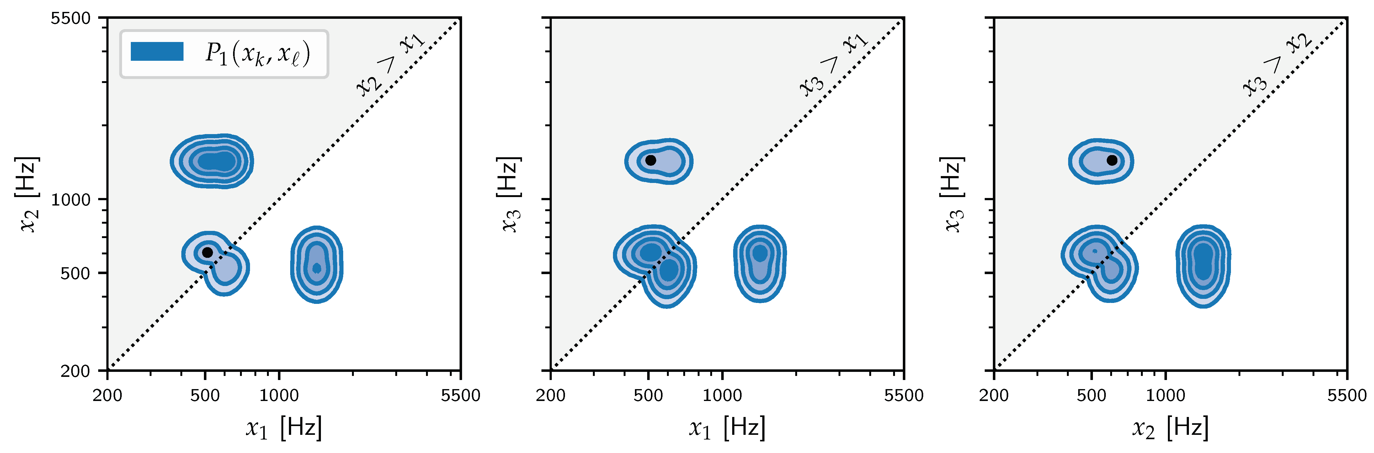
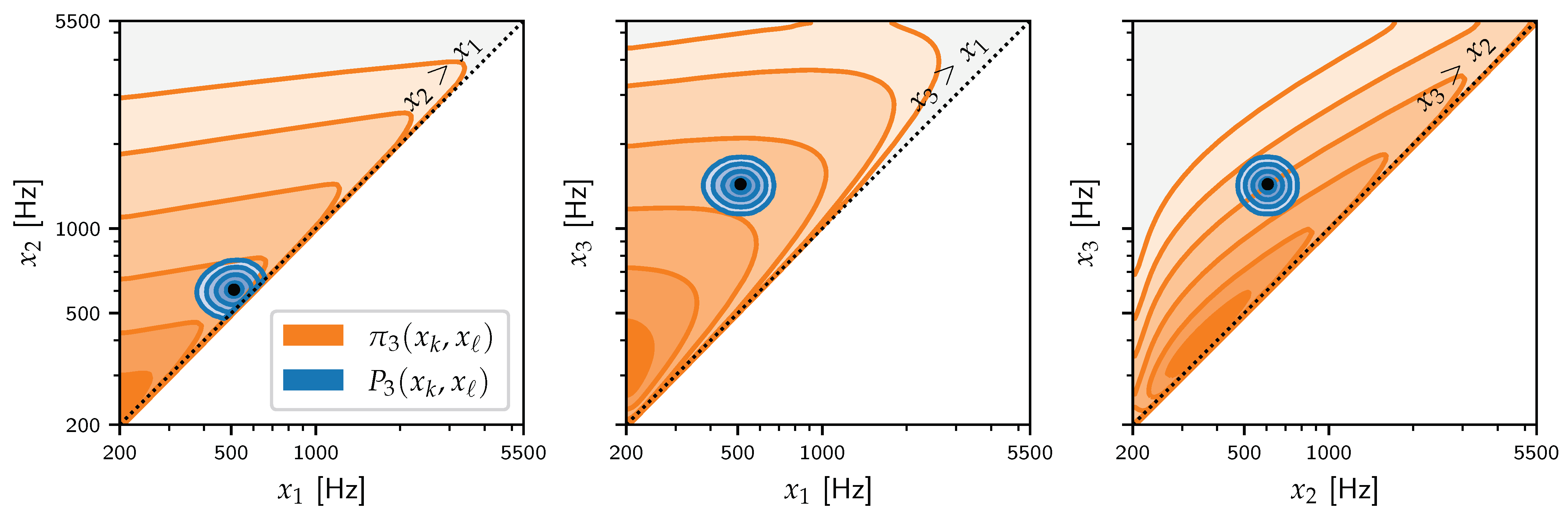
We now present a relatively simple but realistic instance of the problem of measuring resonance frequencies, which will allow us to illustrate the above ideas. The VTR problem consists of measuring human vocal tract resonance (VTR) frequencies $\mathit{x}$ for each of five representative vowel sounds taken from the CMU ARCTIC database [16]. The VTR frequencies $\mathit{x}$ describe the vocal tract transfer function $T\left(x\right)$ and are fundamental quantities in acoustic phonetics [17]. The five vowel sounds are recorded utterances of the first vowel in the words $W=\{\mathsf{shore},\mathsf{that},\mathsf{you},\mathsf{little},\mathsf{until}\}$. In order to achieve high-quality VTR frequency estimates $\widehat{\mathit{x}}$, only the quasi-periodic steady-state part of the vowel sound is considered for the measurement. The data D, thus, consists of a string of highly correlated pitch periods. See Figure 3 for an illustration of these concepts.

The measurement itself is formalized as inference using the probabilistic model (1). The model assumed to underlie the data is the sinusoidal regression model introduced in [18]; due to limited space, we only describe it implicitly. The sinusoidal regression model assumes that each pitch period $\mathit{d}\in D$ can be modeled as

$$d_t=f(t;\mathit{A},\mathit{\alpha },\mathit{x})+\sigma e_t\mathrm{where}{e}_t\sim \mathcal{N}(0,1),(t=1,2,\dots ,T),$$

(22)

where $\mathit{d}={\left\{d_t\right\}}_{t=1}^T$ is a time series consisting of T samples. The model function

$$f(t;\mathit{A},\mathit{\alpha },\mathit{x})=\sum _{k=1}^K[A_{k}cos\left(x_{k}t\right)+A_{K+k}sin\left(x_{k}t\right)]exp\{-{\alpha }_{k}t\}+\sum _{\ell =1}^L{A}_{2K+\ell }{t}^{\ell -1}$$

(23)

consists of a sinusoidal part (first ∑) and a polynomial trend correction (second ∑). Note the additional model parameters $\mathit{\theta }=\{\mathit{A},\mathit{\alpha },\sigma ,L\}$. Formally, given the prior $p\left(\mathit{\theta }\right)$ ([18], Section 2.2), the marginal likelihood $\mathcal{L}\left(\mathit{x}\right)$ is then obtained as $\mathcal{L}\left(\mathit{x}\right)=\int \mathit{\theta }\mathcal{L}(\mathit{x},\mathit{\theta })p\left(\mathit{\theta }\right)$, where the complete likelihood $\mathcal{L}(\mathit{x},\mathit{\theta })$ is implicitly given by (22) and (23). Practically, we just marginalize out $\mathit{\theta }$ from samples obtained from the complete problem $p(D,\mathit{x},\mathit{\theta }|I)$.

For inference, the computational method of choice is nested sampling [1] using the dynesty library [19,20,21,22,23], which scales roughly as $\mathcal{O}\left(K^2\right)$ [24]. Since the VTR problem is quite simple ($H_i\left(K\right)\sim 30\mathrm{nats}$), we only perform single nested sampling runs and take the obtained $log{Z}_i\left(K\right)$ and $H_i\left(K\right)$ as point estimates. Full details on the experiments and data are available at https://github.com/mvsoom/frequency-prior.

5.1. Experiment I: Comparing ${\pi }_2$ and ${\pi }_3$

In Experiment I, we perform a high-level comparison between ${\pi }_2$ and ${\pi }_3$ in terms of evidence (4) and information (6). The values of the hyperparameters used in the experiment are listed in Table 1. We did not include ${\pi }_1$ in this comparison as the label switching problem prevented convergence of nested sampling runs for $K\ge 4$. The $(\mathit{a},\mathit{b})$ bounds for ${\pi }_2$ were based on loosely interpreting the VTRs as formants and consulting formant tables from standard works [25,26,27,28,29,30]. These allowed us to compile bounds up until the fifth formant such that $K_{\max }=5$. For ${\pi }_3$, we simply applied a heuristic where we take $\overline{x_k}=k\times 500\mathrm{Hz}$. We selected $x_0$ empirically (although a theoretical approach is also possible [31]), and $x_{\max }$ was set to the Nyquist frequency. The role of $x_{\max }$ is to truncate ${\pi }_3$ in order to avoid aliasing effects, since the support of ${\pi }_3\left(x_i\right)$ is unbounded from above. We implemented this by using the following likelihood function in the nested sampling program:

$${\mathcal{L}}^{\prime }\left(\mathit{x}\right)=\{\begin{array}{cc}\hfill \mathcal{L}\left(\mathit{x}\right)& \mathrm{if}{x}_k\le x_{\max }\mathrm{for}\mathrm{all}(k=1,2,\dots ,K)\\ 0\hfill & \mathrm{otherwise}.\hfill \end{array}$$

(24)

First, we compare the influence of ${\pi }_2$ and ${\pi }_3$ on model selection. Given $D\in W$, the posterior probability of the number of resonances K is given by the following.

$$p_i\left(K\right)=\frac{Z_i\left(K\right)}{{\sum }_{K^{\prime }}{Z}_i\left(K^{\prime }\right)}(K=1,2,\dots ,K_{\max }).$$

(25)

The results in the top row of Figure 4a are striking: while $p_2\left(K\right)$ shows individual preferences based on D, $p_3\left(K\right)$ prefers $K=K_{\max }$ unequivocally.

Second, in Figure 4b, we compare ${\pi }_2$ and ${\pi }_3$ directly in terms of differences in evidence [$log{Z}_i\left(K\right)$] and uninformativeness [$H_i\left(K\right)$] for each combination $(D,K)$.

Arrows pointing eastward indicate $Z_3\left(K\right)>Z_2\left(K\right)$. The ${\pi }_3$ prior dominates the ${\pi }_2$ prior in terms of evidence, for almost all values of K, indicating that ${\pi }_3$ places its mass in regions of higher likelihood or, equivalently, that the data were much more probable under ${\pi }_3$ than ${\pi }_2$. This implies that the hint of ${\pi }_3$ at more structure beyond $K>K_{\max }$ should be taken serious–we investigate this in Section 5.2.

Arrows pointing northward indicate $H_3\left(K\right)>H_2\left(K\right)$, i.e., ${\pi }_3$ is less informative than ${\pi }_2$, since more information is gained by updating from ${\pi }_3$ to $P_3$ than from ${\pi }_2$ to $P_2$. It is observed that ${\pi }_2$ and ${\pi }_3$ are roughly comparable in terms of (un)informativeness.

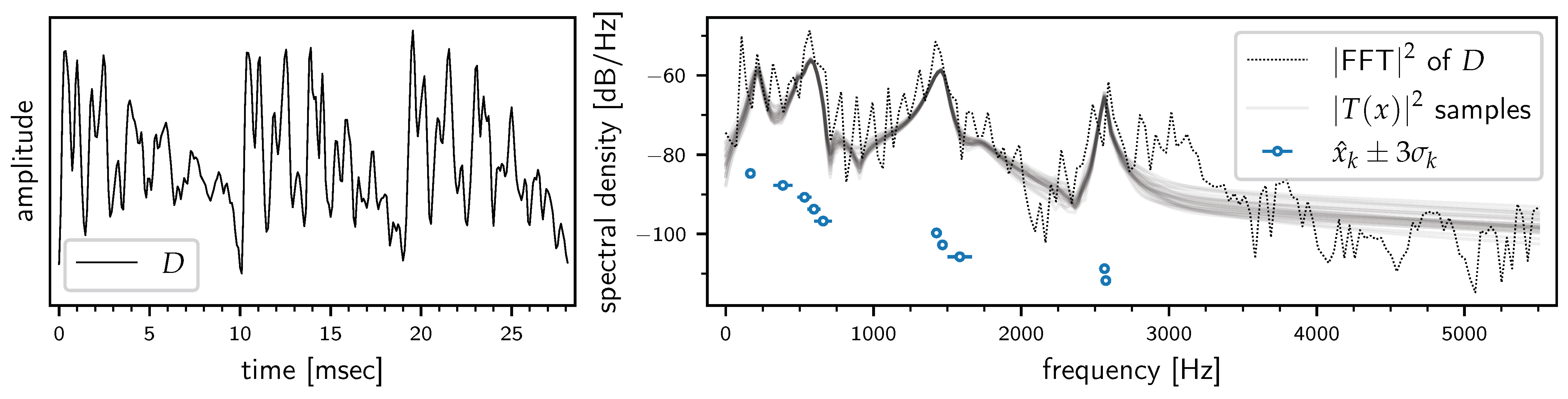
5.2. Experiment II: ‘Free’ Analysis

We now freely look for more structure in the data by letting K vary up until $K_{\max }=10$. This goes beyond the capacities of ${\pi }_1$ (because of the label switching problem) and ${\pi }_2$ (because no data are available to set the $(\mathit{a},\mathit{b})$ bounds). Thus, the great advantage of ${\pi }_3$ is that we can use a simple heuristic to set $\overline{{\mathit{x}}_{\mathbf{0}}}$ and let the model perform the discovering without worrying about convergence issues or the obtained evidence values. The bottom row in Figure 4a shows that model selection for the VTR problem is well-defined, with the most probable values of $K\le 10$, except for $D=\mathsf{until}$. That case is investigated in Figure 3, where the need for more VTRs (higher K) is apparent from the unmodeled broad peak centered at around 3000 Hz in the FFT power spectrum (right panel). Incidentally, this spectrum also shows that spectral peaks are often resolved into more than one VTR, which underlines the importance of using a prior that enables trouble-free handling of multiplets of arbitrary order. A final observation from the spectrum is the fact that the inferred ${\widehat{x}}_k$ differs substantially from the supplied values in $\overline{\mathit{x}}$ (Table 1), which hints at the weak inductive bias underlying ${\pi }_3$.

6. Discussion

It is only when the information in the prior is comparable to the information in the data that the prior probability can make any real difference in parameter estimation problems or in model selection problems.

([32], p. 9)

Although the weakly informative prior for resonance frequencies ${\pi }_3$ is meant to be overwhelmed, its practical advantage (i.e., solving the label switching problem) will nonetheless persist, making a real difference in model selection problems even when “the information in the prior” is much smaller than “the information in the data”. In this sense, ${\pi }_3$ is quite unlike the prior referenced in the above quote. Since it will be overwhelmed, all it has to do is provide a reasonable density everywhere (which it does), be easily parametrizable (which it is), and be easy to sample from (which it is).

Thus, we hope that this prior can enable the use of robust evidence-based methods for a new class of problems, even in the presence of multiplets of arbitrary order. The prior is compatible with off-the-shelf exploration algorithms and solves the label switching problem without any special tuning or post processing. It would be interesting to compare it to other approaches, e.g., [33], especially in terms of exploration efficiency. It is valid for any collection of scale variables that is intrinsically ordered, of which frequencies and wavelengths seem to be the most natural examples. Some examples of recent work where the prior could be applied directly are:

• Nuclear magnetic resonance (NMR) spectroscopy [34];
• Resonant ultrasound spectroscopy (a standard method in material science) [35];
• In the analysis of atomic spectra [36], such as X-ray diffraction [37];
• Accurate modeling of instrument noise (in this case LIGO/Virgo noise) [38];
• Model-based Bayesian analysis in acoustics [39].

References

1. Skilling, J. Nested Sampling for General Bayesian Computation. Bayesian Anal. 2006, 1, 833–859. [Google Scholar] [CrossRef]
2. Green, P.J. Reversible Jump Markov Chain Monte Carlo Computation and Bayesian Model Determination. Biometrika 1995, 82, 711–732. [Google Scholar] [CrossRef]
3. Mark, Y.Z.; Hasegawa-johnson, M. Particle Filtering Approach to Bayesian Formant Tracking. In Proceedings of the IEEE Workshop on Statistical Signal Processing, St. Louis, MO, USA, 28 September–1 October 2003. [Google Scholar]
4. Zheng, Y.; Hasegawa-Johnson, M. Formant Tracking by Mixture State Particle Filter. In Proceedings of the 2004 IEEE International Conference on Acoustics, Speech, and Signal Processing, Montreal, QC, Canada, 17–21 May 2004; Volume 1, pp. 1–565. [Google Scholar] [CrossRef]
5. Yan, Q.; Vaseghi, S.; Zavarehei, E.; Milner, B.; Darch, J.; White, P.; Andrianakis, I. Formant Tracking Linear Prediction Model Using HMMs and Kalman Filters for Noisy Speech Processing. Comput. Speech Lang. 2007, 21, 543–561. [Google Scholar] [CrossRef]
6. Mehta, D.D.; Rudoy, D.; Wolfe, P.J. Kalman-Based Autoregressive Moving Average Modeling and Inference for Formant and Antiformant Tracking. J. Acoust. Soc. Am. 2012, 132, 1732–1746. [Google Scholar] [CrossRef]
7. Shi, Y.; Chang, E. Spectrogram-Based Formant Tracking via Particle Filters. In Proceedings of the (ICASSP ’03), 2003 IEEE International Conference on Acoustics, Speech, and Signal Processing, Hong Kong, China, 6–10 April 2003; Volume 1, p. 1. [Google Scholar] [CrossRef]
8. Deng, L.; Lee, L.J.; Attias, H.; Acero, A. Adaptive Kalman Filtering and Smoothing for Tracking Vocal Tract Resonances Using a Continuous-Valued Hidden Dynamic Model. IEEE Trans. Audio Speech Lang. Process. 2007, 15, 13–23. [Google Scholar] [CrossRef]
9. Luberadzka, J.; Kayser, H.; Hohmann, V. Glimpsed Periodicity Features and Recursive Bayesian Estimation for Modeling Attentive Voice Tracking. Int. Congr. Acoust. 2019, 9, 8. [Google Scholar]
10. Stephens, M. Dealing with Label Switching in Mixture Models. J. R. Stat. Soc. Ser. (Stat. Methodol.) 2000, 62, 795–809. [Google Scholar] [CrossRef]
11. Celeux, G.; Kamary, K.; Malsiner-Walli, G.; Marin, J.M.; Robert, C.P. Computational Solutions for Bayesian Inference in Mixture Models. arXiv 2018, arXiv:1812.07240. [Google Scholar]
12. Celeux, G.; Fruewirth-Schnatter, S.; Robert, C.P. Model Selection for Mixture Models - Perspectives and Strategies. arXiv 2018, arXiv:1812.09885. [Google Scholar]
13. Bretthorst, G.L. Bayesian Spectrum Analysis and Parameter Estimation; Springer: Berlin/Heidelberg, Germany, 1988. [Google Scholar]
14. Knuth, K.H.; Skilling, J. Foundations of Inference. Axioms 2012, 1, 38–73. [Google Scholar] [CrossRef] [Green Version]
15. Jaynes, E.T. Prior Probabilities. IEEE Trans. Syst. Sci. Cybern. 1968, 4, 227–241. [Google Scholar] [CrossRef]
16. Kominek, J.; Black, A.W. The CMU Arctic Speech Databases. In Proceedings of the Fifth ISCA Workshop on Speech Synthesis, Pittsburgh, PA, USA, 14–16 June 2004. [Google Scholar]
17. Van Soom, M.; de Boer, B. A New Approach to the Formant Measuring Problem. Proceedings 2019, 33, 29. [Google Scholar] [CrossRef] [Green Version]
18. Van Soom, M.; de Boer, B. Detrending the Waveforms of Steady-State Vowels. Entropy 2020, 22, 331. [Google Scholar] [CrossRef] [PubMed] [Green Version]
19. Speagle, J.S. Dynesty: A Dynamic Nested Sampling Package for Estimating Bayesian Posteriors and Evidences. arXiv 2019, arXiv:1904.02180. [Google Scholar] [CrossRef] [Green Version]
20. Feroz, F.; Hobson, M.P.; Bridges, M. MULTINEST: An Efficient and Robust Bayesian Inference Tool for Cosmology and Particle Physics. Mon. Not. R. Astron. Soc. 2009, 398, 1601–1614. [Google Scholar] [CrossRef] [Green Version]
21. Neal, R.M. Slice Sampling. Ann. Stat. 2003, 31, 705–767. [Google Scholar] [CrossRef]
22. Handley, W.J.; Hobson, M.P.; Lasenby, A.N. POLYCHORD: Nested Sampling for Cosmology. Mon. Not. R. Astron. Soc. 2015, 450, L61–L65. [Google Scholar] [CrossRef]
23. Handley, W.J.; Hobson, M.P.; Lasenby, A.N. POLYCHORD: Next-Generation Nested Sampling. Mon. Not. R. Astron. Soc. 2015, 453, 4384–4398. [Google Scholar] [CrossRef] [Green Version]
24. Buchner, J. Nested Sampling Methods. arXiv 2021, arXiv:2101.09675. [Google Scholar]
25. Peterson, G.E.; Barney, H.L. Control Methods Used in a Study of the Vowels. J. Acoust. Soc. Am. 1952, 24, 175–184. [Google Scholar] [CrossRef]
26. Hillenbrand, J.; Getty, L.A.; Clark, M.J.; Wheeler, K. Acoustic Characteristics of American English Vowels. J. Acoust. Soc. Am. 1995, 97, 3099–3111. [Google Scholar] [CrossRef] [Green Version]
27. Vallée, N. Systèmes Vocaliques: De La Typologie Aux Prédictions. Ph.D. Thesis, Université Stendhal, Grenoble, France, 1994. [Google Scholar]
28. Kent, R.D.; Vorperian, H.K. Static Measurements of Vowel Formant Frequencies and Bandwidths: A Review. J. Commun. Disord. 2018, 74, 74–97. [Google Scholar] [CrossRef]
29. Vorperian, H.K.; Kent, R.D.; Lee, Y.; Bolt, D.M. Corner Vowels in Males and Females Ages 4 to 20 Years: Fundamental and F1–F4 Formant Frequencies. J. Acoust. Soc. Am. 2019, 146, 3255–3274. [Google Scholar] [CrossRef] [PubMed]
30. Klatt, D.H. Software for a Cascade/Parallel Formant Synthesizer. J. Acoust. Soc. Am. 1980, 67, 971–995. [Google Scholar] [CrossRef] [Green Version]
31. de Boer, B. Acoustic Tubes with Maximal and Minimal Resonance Frequencies. J. Acoust. Soc. Am. 2008, 123, 3732. [Google Scholar] [CrossRef] [Green Version]
32. Bretthorst, G.L. Bayesian Analysis. II. Signal Detection and Model Selection. J. Magn. Reson. 1990, 88, 552–570. [Google Scholar] [CrossRef]
33. Buscicchio, R.; Roebber, E.; Goldstein, J.M.; Moore, C.J. Label Switching Problem in Bayesian Analysis for Gravitational Wave Astronomy. Phys. Rev. D 2019, 100, 084041. [Google Scholar] [CrossRef] [Green Version]
34. Wilson, A.G.; Wu, Y.; Holland, D.J.; Nowozin, S.; Mantle, M.D.; Gladden, L.F.; Blake, A. Bayesian Inference for NMR Spectroscopy with Applications to Chemical Quantification. arXiv 2014, arXiv:1402.3580. [Google Scholar]
35. Xu, K.; Marrelec, G.; Bernard, S.; Grimal, Q. Lorentzian-Model-Based Bayesian Analysis for Automated Estimation of Attenuated Resonance Spectrum. IEEE Trans. Signal Process. 2019, 67, 4–16. [Google Scholar] [CrossRef]
36. Trassinelli, M. Bayesian Data Analysis Tools for Atomic Physics. Nucl. Instruments Methods Phys. Res. Sect. Beam Interact. Mater. Atoms 2017, 408, 301–312. [Google Scholar] [CrossRef] [Green Version]
37. Fancher, C.M.; Han, Z.; Levin, I.; Page, K.; Reich, B.J.; Smith, R.C.; Wilson, A.G.; Jones, J.L. Use of Bayesian Inference in Crystallographic Structure Refinement via Full Diffraction Profile Analysis. Sci. Rep. 2016, 6, 31625. [Google Scholar] [CrossRef] [PubMed] [Green Version]
38. Littenberg, T.B.; Cornish, N.J. Bayesian Inference for Spectral Estimation of Gravitational Wave Detector Noise. Phys. Rev. D 2015, 91, 084034. [Google Scholar] [CrossRef] [Green Version]
39. Xiang, N. Model-Based Bayesian Analysis in Acoustics—A Tutorial. J. Acoust. Soc. Am. 2020, 148, 1101–1120. [Google Scholar] [CrossRef] [PubMed]
Figure 1. The exchange symmetry of the posterior P 1 ( x ) for a well-determined instance of the VTR problem from Section 5 with K : = 3 . The pairwise marginal posteriors P 1 ( x k , x ) are shown using the isocontours of kernel density approximations calculated from posterior samples of x . For each panel, the diagonal x k = x is plotted as a dotted line, and the ordered region R 3 ( x 0 ) is shaded in grey. The black dot marks the mean of the primary mode for this problem.
Psf 03 00002 g001
Figure 2. Contraction of prior ( π 3 ) to posterior ( P 3 ) for the application of π 3 to the VTR problem used in Figure 1. The pairwise marginal prior π 3 ( x k , x ) is obtained by integrating out the third frequency; for example, π 3 ( x 1 , x 2 ) = d x 3 π 3 ( x ) . Unlike P 1 in Figure 1, P 3 exhibits only a single mode that coincides with the primary mode as marked by the black dot.
Psf 03 00002 g002
Figure 3. The VTR problem for the case ( D : = until , K : = 10 ) . Left panel: The data D, i.e., the quasi-periodic steady-state part, consist of 3 highly correlated pitch periods. Right panel: Inferred VTR frequency estimates { x ^ k } k = 1 K for K : = 10 at 3 sigma. They describe the power spectral density of the vocal tract transfer function | T ( x ) | 2 , represented here by 25 posterior samples and compared to the Fast Fourier Transform (FFT) of D. All x ^ k are well resolved, and most have error bars too small to be seen on this scale.
Psf 03 00002 g003
Figure 4. (a) Model selection in Experiment I (top row) and Experiment II (bottom row). (b) In Experiment I, π 2 and π 3 are compared in terms of evidence [ log Z i ( K ) ] and uninformativeness [ H i ( K ) ] for each ( D , K ) . The arrows point from π 2 to π 3 and are color-coded by the value of K. For small values of K, the arrow lengths are too small to be visible on this scale.
Psf 03 00002 g004