Abstract
The United States is experiencing a large growth in the solar sector. The U.S. solar power capacity has grown from 0.34 Gigawatts (GW) in 2008 to an estimated 97.2 GW today. However, some states have had difficulty installing large scale solar farms due to concerns regarding geographic location, political climate, or economic factors. Kentucky (KY) is one of the states which is below the national average for solar energy production. However, KY contains a wealth of potential for these types of farms with decent solar irradiation levels and large tracts of unused land for solar farms. For the study, this paper selects three representative areas of KY by using PVWatts and topographical maps which can theoretically produce enough electricity so that KY can meet or exceed the national generation percentage average (2.3% or 2.06 TWh annually in KY’s case). The study analyzes the economic feasibility of solar photovoltaic systems (PV) farms in terms of Cumulative Cash Flow ($) and Payback Time (Year) by using the Cost of Renewable Energy Spreadsheet Tool (CREST). Furthermore, this paper estimates the Average/Median/High output power (kWh) annually for the scenario among three areas in Kentucky, Smithland, Hickman, and Falls of Rough. In this theoretical scenario, an average 2.27 TWh would be generated annually which exceeds the national generation percentage average. Furthermore, by the sixth year, the cumulative cash flow would exceed the breakeven point, proving the feasibility of these solar farms. The annual average power generation estimates for the areas of Smithland, Hickman, and Falls of Rough are 0.3741 TWh, 1.1628 TWh, and 0.731 TWh respectively. The average profit per MWh estimates for the areas of Smithland, Hickman, and Falls of Rough are $11,130.12/MWh, $10,742.46/MWh, and $11,392.01/MWh respectively. According to CREST, the final cumulative cash flow, after the 25-year life span of the panels, would be approximately $624,566,720.
1. Introduction
Despite many beliefs, solar energy is feasible in Kentucky. While the state may not have the solar irradiation rates of places like Arizona, or the number of incentives as states like California [1], Kentucky does receive an adequate amount of sunlight to make Solar PV installation profitable. There are large tracts of unused land perfect for large scale solar that many more urban areas lack [2,3]. In addition, while Kentucky lacks large scale solar, small scale solar has been steadily growing, and sentiment has slowly been shifting in favor of the generation method, as shown in Figure 1 [4,5,6,7]. The objective of this paper is to demonstrate the feasibility of large-scale solar generation in Kentucky by designing several large-scale solar farms in the state and conducting a financial analysis of these designs.
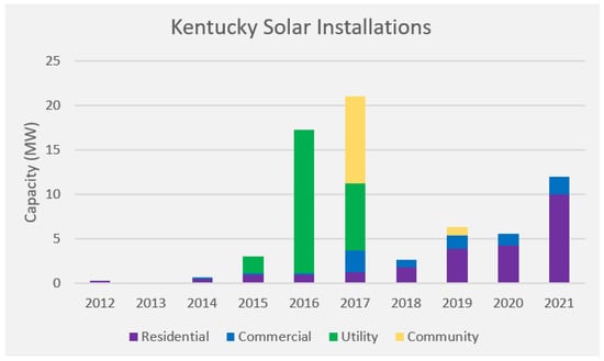
Figure 1.
KY Annual Solar Installations by Sector [6].
To understand the future of solar energy within Kentucky, the current situation must first be examined. This section examines the historical and current role solar fills in Kentucky’s energy grid. Despite the rising favorability of solar, Kentucky is a state that historically has been highly coal dependent. Even in 2020, nearly three quarters of Kentucky’s electricity was generated from coal, as shown in Figure 2 [8,9].
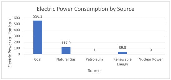
Figure 2.
Electric power sector consumption by source for Kentucky [8].
Coal mining was a prosperous industry in Kentucky for decades, and it was a semi-reliable source of work despite the dangerous conditions. While the job was looked down upon at the time, many people in Kentucky today have romanticized the role of coal miners and are now opposed to renewable energy sources because they see them as a threat to their “way of life” despite coal mining being a declining industry [10].
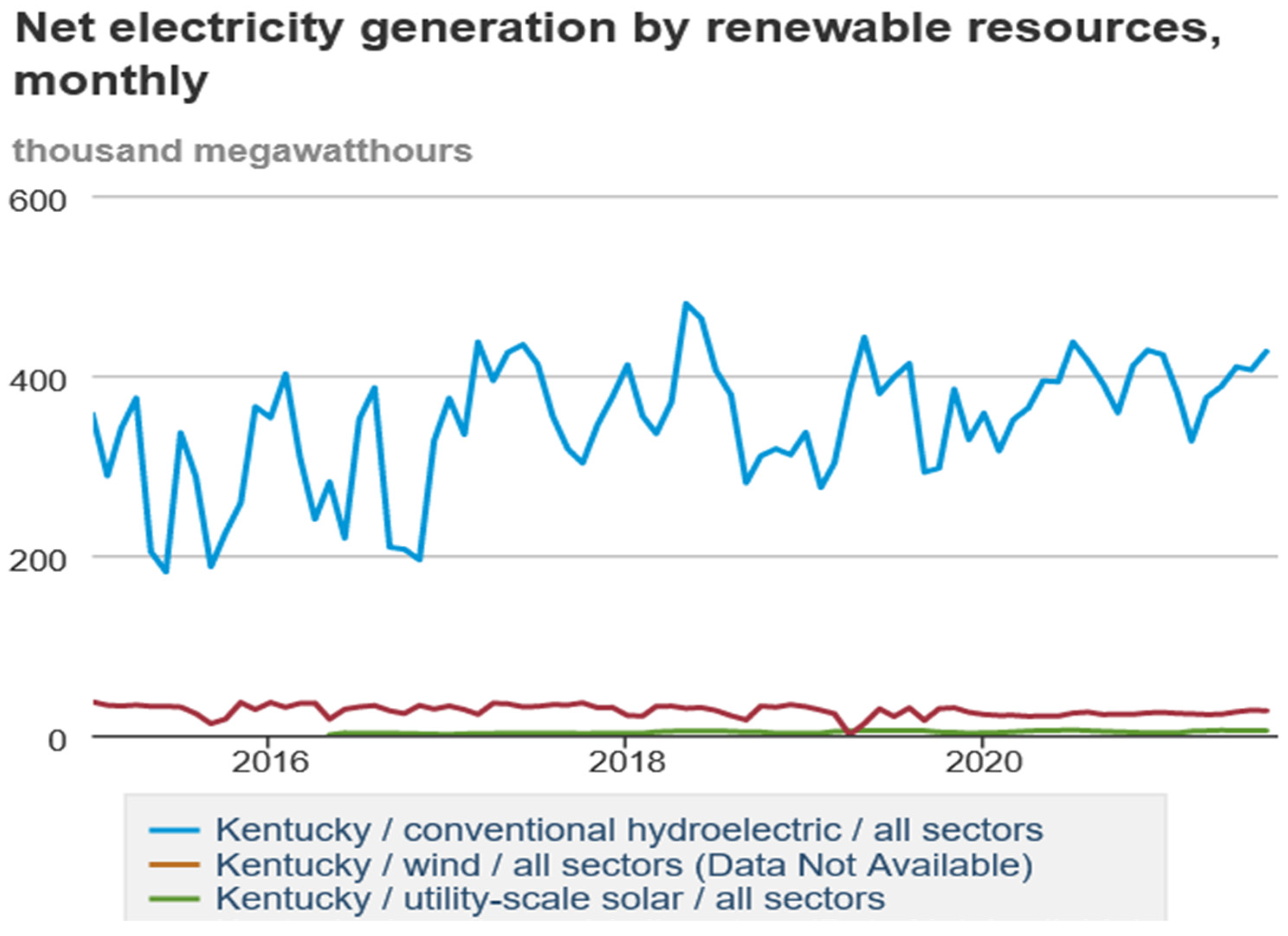
This may be why, compared to many states, there are few incentives for the people of Kentucky to invest in solar farms. There is little to no incentive for large scale solar to be implemented within the state. In fact, there are only two instances of what could be called utility grade solar in Kentucky. In each case electrical generation compared to load is miniscule, as shown in Figure 3 where the net generation of utility level renewable energy is graphed.
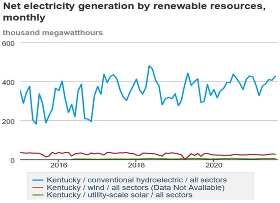
Figure 3.
Net electricity generation by renewable resources monthly in Kentucky [8].
However, there have been some incentives for individuals to invest in solar. In 2008 the state passed legislation requiring all electric cooperatives and corporations—except TVA utilities—to offer Net Metering to all individuals with PV, wind, biomass, biogas, or hydroelectric systems. This would allow independent individuals to sell back excess power generated by solar panels on their property. The cap was originally set at 30 kW but was raised to 45 kW by KY Senate Bill 100 as of 2020 [11]. Envirowatts is a program where consumers pay extra to purchase green energy, and that excess is invested back into renewable energy sources, but it is extremely limited [12,13]. In addition to this, there are some easements, tax incentives, and a grant for solar installed on farms. In total there are 26 programs to assist with the costs of solar generation in Kentucky, only seven of which are unique to Kentucky. The rest are federal policies and incentives [2,14]. In addition to these twenty-six programs, there is also the cooperative solar opportunity of Solar Farm One, which will be addressed in another section.
To truly grow Kentucky’s solar energy infrastructure, political changes need to occur. The state government needs to incentivize the industry to bring larger companies to the area. Many other industries already relocate factories and production facilities that cannot be outsourced to other countries to Kentucky because of the lower property taxes and labor costs. With added financial incentives to assist with the initial set up costs, solar in Kentucky could be a very profitable industry, and the new market could generate jobs to replace the coal jobs that are steadily declining.
2. Materials and Methods
2.1. Analysis of Solar PV Potential in Kentucky
2.1.1. The Current of Solar in the KY State
While the solar industry in Kentucky is severely underdeveloped in comparison to other areas of the country, there are a few ongoing solar initiatives and operating solar farms that show the viability of solar in Kentucky. Cooperative Solar was implemented by rural member owned electric cooperatives to use pooled resources to create Solar Farm One. There is also some Corporate Solar within the state where investor-owned corporations have installed solar for profit, such as Duke Energy. Small Scale Solar is the solar generated by homeowners and individuals in the Kentucky for their own personal use or to sell back to the state.
Cooperative Solar
Solar Farm One is a cooperative solar endeavor, meaning that member owned cooperatives participate in this program for the benefit of their members. It is located in Winchester Kentucky and maintained by EKPC. It is a 60-acre solar farm with over 32,300 panels, some fixed, others 2-axis tracking. Panels are “sold” to consumers from cooperatives. The consumer pays for the panel and upkeep. Then, all electricity generated is credited to their bill [15].
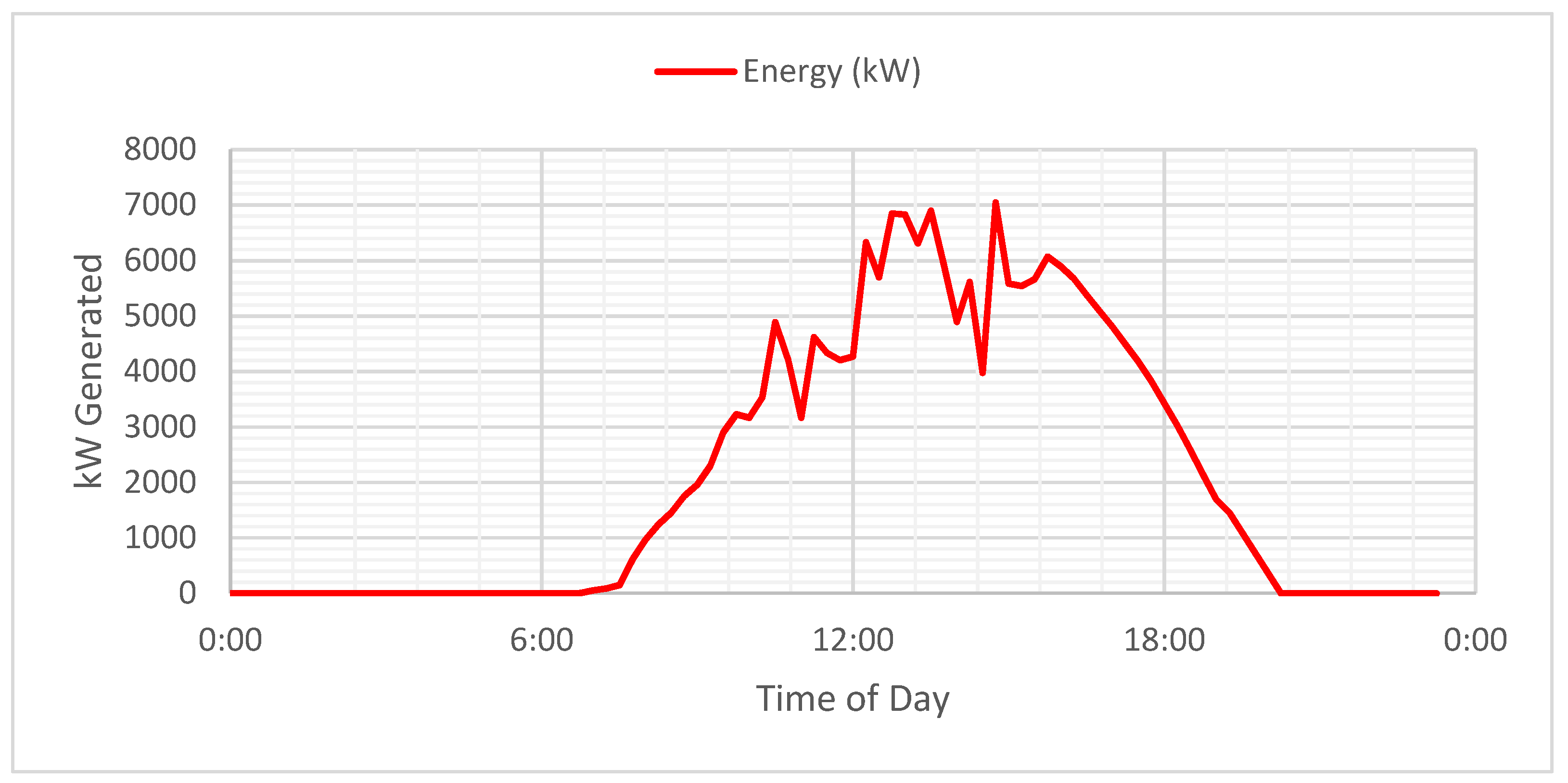
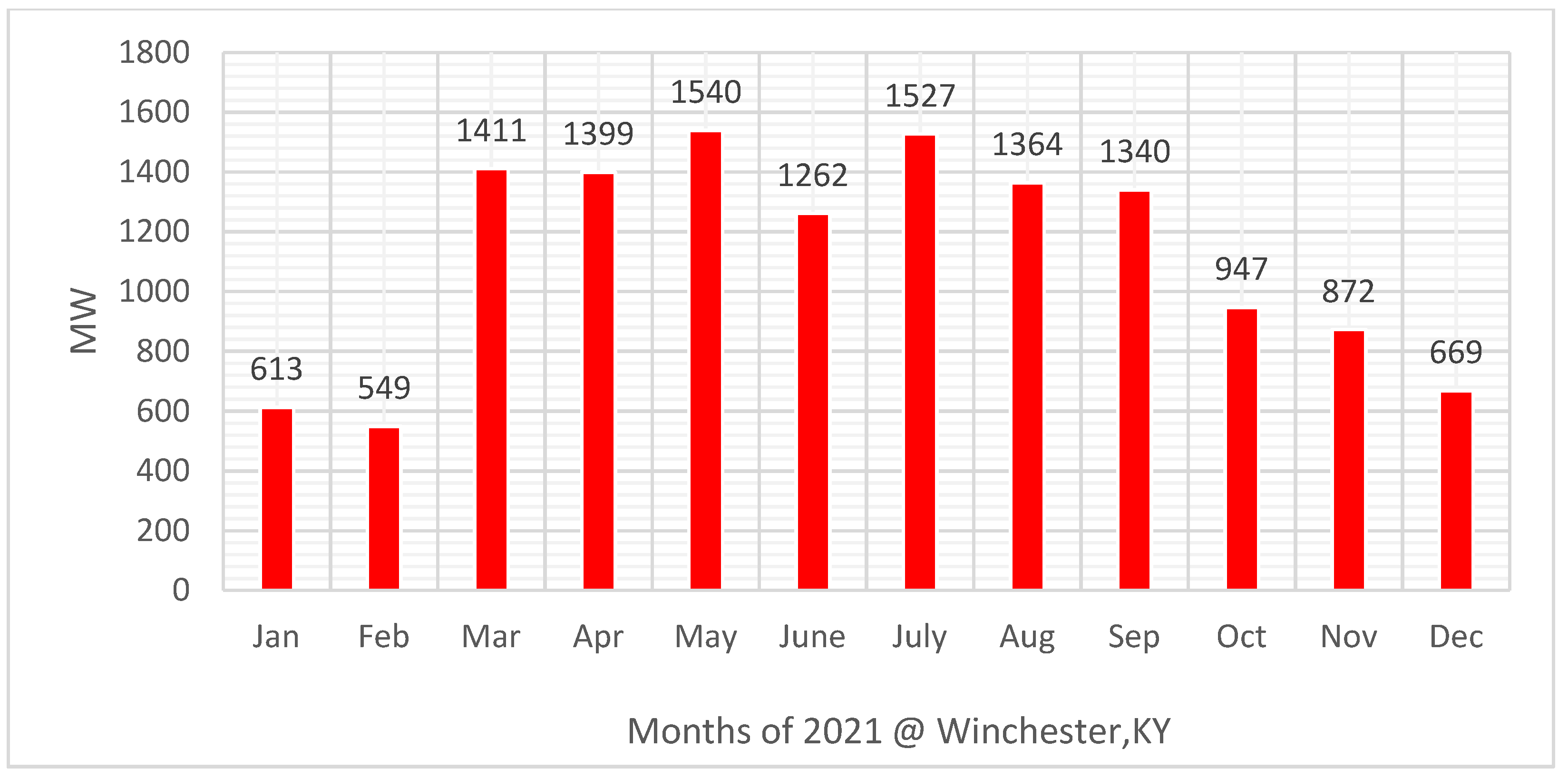
This solar farm began operating on 25 October 2017, and since then it has generated 12.5 GWh. The program is praised for assisting the average citizen to support and benefit from renewable energy and for being an affordable way to invest in solar panels. The farm also provides real time data so that anyone interested in their program can access their generation data. This data is displayed in Figure 4 (output on 3 June 2022) and Figure 5 (2021 yearly data). This allows consumers to see how much power was generated hourly on any given day, daily any given month, and monthly any given year [15].
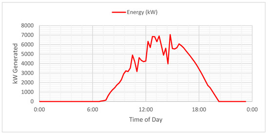
Figure 4.
Daily output of Solar Farm One: Winchester, KY on 3 June 2022 [15].

Figure 5.
Yearly Output of Solar Farm One: Winchester, KY for 2021 [15].
Corporate Solar
Corporate solar in Kentucky is the investor-owned farms that are for profit. At the time of Duke’s solar farm’s construction, Duke Energy was one of the United States’ top five renewable energy companies. Duke Energy services parts of Kentucky and Ohio, but before this solar farm most of their renewable energy efforts had been focused in Ohio. However, they decided to add some form of renewable energy into their repertoire for Northern Kentucky because Duke Energy previously only had coal-fire and natural gas power-plants in-state [16,17].
They decided to build three power plants with the goal of reaching a 6.8 MW capacity. The plan was to have two solar farms in Kenton County, Walton Solar Power Plant One and Walton Solar Power Plant Two, on different parts of the same 60-acre tract of land. Combined, there would be approximately 19,000 solar panels with a 4 MW capacity [16,17]. The farm finally opened on 14 December 2017, as a singular power plant with 17,024 panels and a slightly smaller capacity. The other plant was the Crittenden Solar Power Plant in Grant County, which was meant to house approximately 12,500 panels with a 2.7 MW capacity. The final completed farm did not meet this goal, housing only 11,500 panels. This farm also started its operation on 14 December 2017 [16,17].
Small Scale Solar
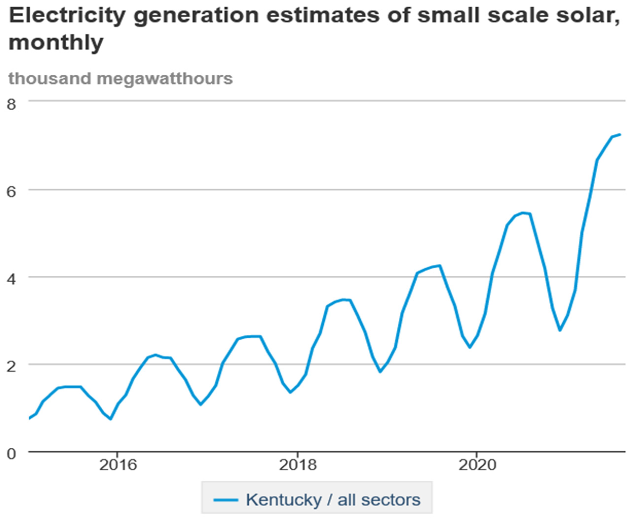
Small scale solar is defined by the EIA as a system that generates less than a singular megawatt [18]. While large scale solar is important, in Kentucky small scale solar is a far more rapidly growing industry. This is partially because Kentucky is an extremely rural state. Despite the massive expansion of rural electrification in the past seventy-five years, there are still regions in Kentucky where if someone builds there, they would be far removed from any form of electrical infrastructure and would either pay heavily to obtain that infrastructure or find an alternative. For this reason, roof-top solar and off-grid solar panels are growing in popularity. They are being installed on homesteads and in hunting cabins. Some people will install them as an alternative winter back-up in the place of traditional gas generators, since snowstorms can cause power loss for weeks depending on where one lives [5,19,20]. As shown in Figure 6, small scale solar generation has quadrupled since 2015 [8].
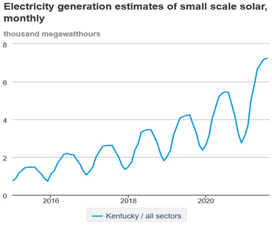
Figure 6.
Electricity generation estimates for small scale solar in Kentucky [8].
In addition to this, businesses and farms have begun to have solar panels installed to reduce electricity costs. For example, the Hemphill Community Center claims their solar panels and their newly reduced electricity bill are the reason they were able to stay open [21]. They had 66 panels installed (approximately 24 kW) and estimate that they save over $300 a month. Plus, Dotson Farms had 15 kW worth of solar panels installed, and the farm made a 10-year contract with the Tennessee Valley Authority to buy their electricity back at $0.14/kW. They have effectively offset their electricity bill with their solar income [21].
2.1.2. The Future of Solar in the KY State
According to the National Renewable Energy Laboratory (NREL), the factor that will truly determine the rate of growth for solar in Kentucky will be the cost of photovoltaic (PV) panels [5]. In a 2017 study on Projections of Distributed Photovoltaic Adoption in Kentucky through 2040, the distributed PV capacity in Kentucky was estimated based on the price of PV panels—low cost, mid cost, and high cost. This study mainly focused on the rooftop solar potential in Kentucky, and it is estimated by the NREL that the Distributed Photovoltaics Capacity (DPC) will range from 162 MW to 3160 MW in 2040, which would be 211.9 GWh/year to 4111.6 GWh/year. There is currently approximately 130 million square meters of roof area suitable for solar, which is the base area used for this study. The study is estimating that somewhere between 1–18% of the technical potential will be in use by 2040, as showcased in Table 1 [5].

Table 1.
Installed DPV capacity (MWdc)and energy generation in Kentucky [5].
Another promising upcoming source of solar energy in the state is the campaign to transform strip mines into solar farms. Strip mining was a common practice in Eastern Kentucky for decades. The practice is being slowly phased out due to the intense damage it does to the surrounding environment, wildlife, and water sources. In an attempt to reclaim some of these sites, Kentucky Governor Andy Beshear has approved $600,000 in tax incentives to Savion. By 2024, Savion hopes to have constructed a 200 MW solar farm that would power 33,000 Kentucky homes. Construction should start this year. [22].
Solar is a topic that is slowly gaining more and more traction, which can be showcased by these large new projects and by the number of feasibility studies being performed. Similar studies to this one has been done in the past regarding solar feasibility, this one differs primarily due to location, scale, and factors taken into consideration. Solar feasibility studies have been focused on Kentucky before, such as Analysis of Photovoltaic Energy in the Eastern Kentucky Region and the Residential Financial Feasibility and Installation of solar panels in a residential setting: A feasibility study for a Southern US City, but these studies primarily focused was on small scale or residential solar, whereas this focuses on utility scale solar. [3,7] Other studies such as Feasibility Study of Economics and Performance of Solar Photovoltaics at the Price Landfill Site in Pleasantville, New Jersey—a study that also utilized the one of the same programs as this paper—do study large scale solar feasibility, but the location is different. There is not the same terrain, load constraints, and socio-economic factors at play in New Jersey as there are in Kentucky. [23] The same is true with Implementation of a large-scale solar photovoltaic system at a higher education institution in Illinois, USA. It also used SAM and had a similar process as this paper, but involved a different location, and the focus was on payback period for a university project, instead of output. [24]
2.2. Approach
To prove that solar was feasible and could even be profitable in Kentucky, this paper creates a rough estimate for the output of three solar farms in Kentucky. A side goal was to design farms large enough that their output would theoretically push Kentucky’s solar electricity generation over the national average. The percentage of electricity in the United States that is generated via solar energy is 2.3% according to the Energy Information Association (EIA), while the Kentucky average is 0.2% as of 2020. That means to meet the national average, an additional 2.1% or 1.88 TWh of KY’s total electricity consumption would have to be generated via solar. This amount of solar generation is unprecedented in Kentucky [7,25].
Three locations were chosen for potential solar farms. There are many considerations when choosing the location for a solar farm. This paper utilizes similar criteria, with minor differences to account for the differences in location. The primary ones are listed in Table 2 below:
Table 2.
Parameter Definitions.
- (1)
- Terrain
- (2)
- Solar Irradiance
- (3)
- Cost and Size
- (4)
- Proximity to pre-existing infrastructure.
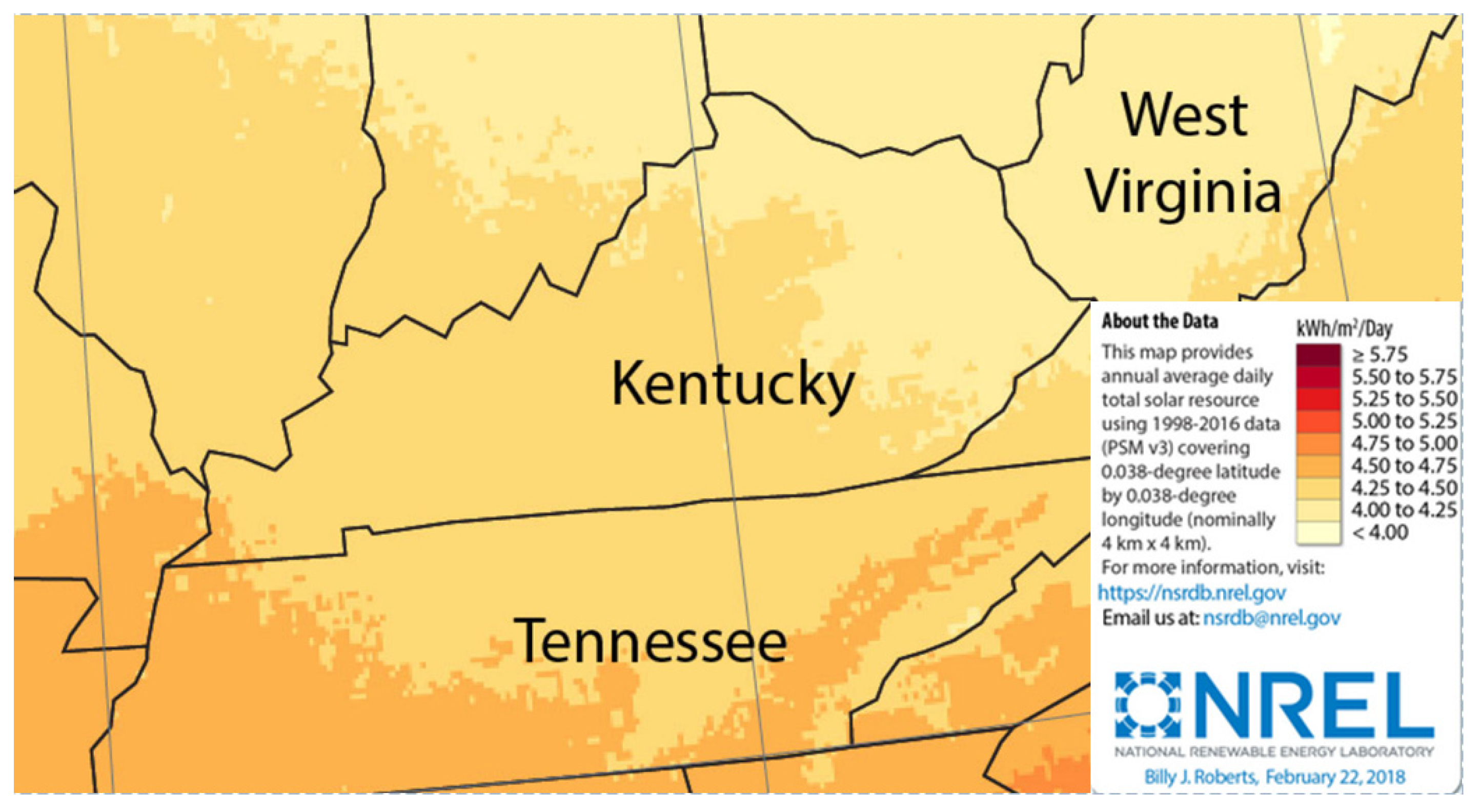
Consideration (1) Terrain. Eastern Kentucky is mountainous, which would add an additional layer of difficulty to the construction of a solar farm. There would be additional difficulties transporting supplies and equipment up narrow, winding roads. It would be difficult to locate or create a flat field to station the sheer volume of panels needed for this size of solar farm. This area is densely wooded as well meaning there will be a need to clear an area for the farm to be constructed. However, the mid and western parts of the state are flatter, less densely wooded, and typically have better roadways. Another consideration that falls under Terrain is flood plains. Flooding is common in Kentucky and building on a flood plain could cause costly damage down the line. Topographical maps (Figure 7), Google Earth, and PVWatts were used to determine the suitability of the properties [25,26,27].

Figure 7.
Solar irradiation data from NREL displayed on map for various regions of Kentucky.
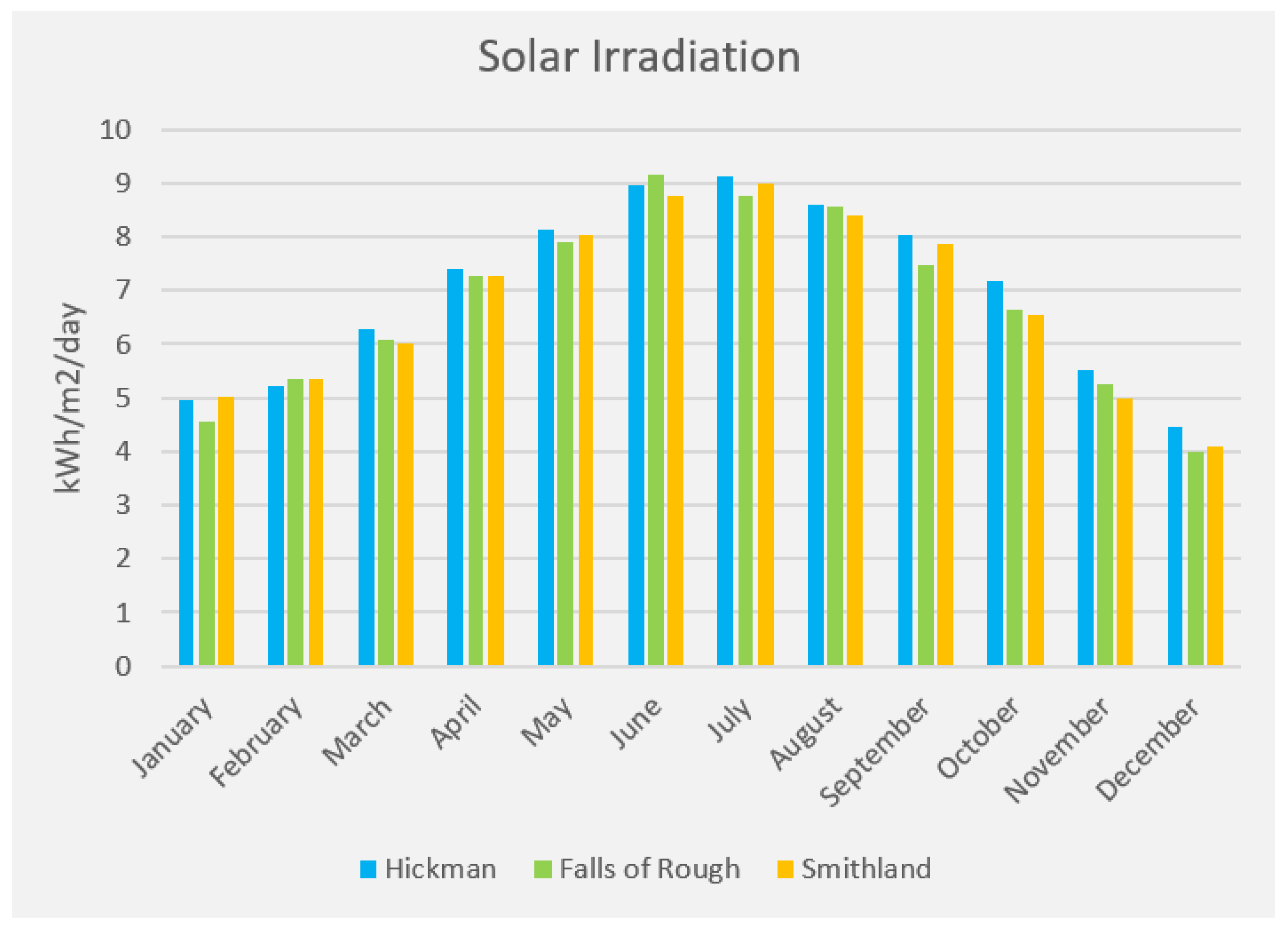
Consideration (2) Solar Irradiation. Kentucky does not have the solar irradiation numbers that states like Arizona or California have, but they are on par with states like Georgia, which almost meets the national average for generation. Solar irradiation data was pulled from the National Renewable Energy Laboratory for various parts of the state to determine which region had the highest kWh/m2/day. Some of this data is shown in Figure 8. The NREL’s excel files for solar data and PVWatts were used during this step [27].
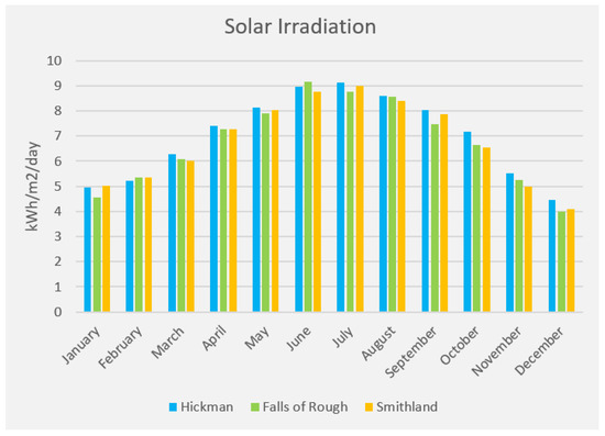
Figure 8.
Solar irradiation data from the chosen three areas (Hickman, Falls of Rough, and Smithland of KY) on a graph [1,27].
Consideration (3) Cost and Size. The western area of the state was found to have the highest numbers. Therefore, the search began in western Kentucky for areas that could house solar. Since the focus of this paper is large scale solar farms, only properties over 500 acres for sale were examined [27]. The cost of the property was also taken into consideration, as the high price per acreage would affect the upfront costs of creating the solar farm when it came time to complete the financial analysis portion.
Consideration (4) Pre-existing infrastructure. Areas near pre-existing power plants or along large transmission lines were preferred since those areas will have a grid better prepared to handle large loads. In addition to that, if a potential solar farm had a coal or hydroelectric power plant nearby, that plant could compensate for times when the solar farms output would be insufficient, such as at night.
Taking these factors into account, three locations were chosen as potential sites for solar farms. These sites were chosen based on the factors listed above and property availability in Kentucky at the start of this study. Over 30 locations were found for sale in Western Kentucky that were large enough to house a solar farm of this magnitude and were in areas with appropriately high solar irradiation. Some were eliminated due the first factor terrain. Topographical maps showed that the areas contained undesirable natural features such as ridges or sharp slopes. In other cases, proximity to rivers and flood plains were an issue. Some were eliminated as well due to price, since a financial analysis is also being completed. Out of the remaining properties, those located closest to existing infrastructure were chosen. Location 1 (Smithland) was located near multiple coal and hydroelectric power plants. Location 2 (Hickman) was located relatively close to a coal fired plant, and Location 3 (Falls of Rough) was near one of the largest transmission lines in the state and a biofuel power plant [7].
2.3. Modeling
2.3.1. System Advisor Model (SAM) and Cost of Renewable Energy Spreadsheet Tool (CREST)
The System Advisor Model (SAM) and PVWatts were used to perform the mathematical modeling. SAM has multiple modeling options. The one used for this study was the Detailed PV Model for solar generation analysis in tandem with the Cost of Renewable Energy Spreadsheet Tool (CREST), which was used to analyze the financials [28].
Step (1) Find best location by using PVWatts, Google Earth, topographical maps, and electrical generation and transmission maps, while taking geographical location and features, solar irradiation, size, and proximity to existing infrastructure into account [26,27].
Step (2) Enter parameters into SAM for estimated annual power output (TWh) calculations and graph generation [29].
Step (3) Enter variables requested by the financial model, which include degradation rate, income tax rates, and incentives [30].
2.3.2. SAM Parameters
There are a variety of factors to consider when determining solar generation output (kWh produced). Some of the factors the model addresses are covered in this section. Yearly Solar Irradiance is one, as well as the sun’s position. The tracking system used is key. Since the selected solar panels use two axis tracking, the surface tilt and azimuth angles follow the sun’s zenith and azimuth angles. AOI (angle of incidence) correction is used to adjust the direct beam irradiance to account for reflection losses. Based on the POA irradiance incident on the module cover, an AOI correction is added to “adjust the direct beam irradiance to account for reflection losses” [29]. There is also the angle of refraction to consider, as well as transmittance through the glass and effective transmittance. The cell temperature, nameplate DC rating, system losses, DC system size, and efficiency of the inverter are also considerations. Other variables include module type, DC to AC ratio, and ground coverage ratio [29]. These considerations are similar to those used in Feasibility Study on a Large Scale Solar PV System. However, Gauli only accounts for losses due to temperature, cables, and invertors, whereas this model accounts for losses due to soiling, shading, snow, mismatch, wiring, connections, light induced degradation, nameplate rating, and age [31].
Many of these factors are determined by the solar panels used and location. For example, there are various categories under system losses to enter loss percentages based on the type of loss. Many loss parameters were left at their default value. However, some were altered, such as snow. The default losses due to snow were originally 0%. However, snow is common in Kentucky, and some system losses will occur because of it [29].
The program outputs a variety of different graphs. The System AC power output (Pgen) of the theoretical solar arrays (kWh) was the main focus. There are many calculations that take place to arrive at this value [29,32,33]. Below are some of the key equations:
This equation takes the number of invertors into account (Ninv), the AC output of a single invertor (Pac), total AC power loss (Lac), and curtailment and availability losses (Ladjust). Total AC power loss is affected by transformer losses (Ltransformer) and wiring losses (Lacwiring) [29,32,33].
The AC Invertor Output () is determined using the Sandia Invertor model [29,32,33].
In this scenario, refers to the maximum power dc power out, and is the power consumption during operation. and are DC string voltage and the nominal DC voltage. C0, C1, C2, and C3 are the curvature between AC and DC power, the variation coefficient of with DC input voltage, the variation coefficient of with DC input voltage, and the variation coefficient of C0 with DC input voltage respectively [29,32,33]. Then, to find Pac the following equation would be utilized:
In this equation, Pac,0 is the maximum AC power output [29,32,33].
SAM/PVWatts also provides three estimates of annual output—a conservative estimate, an average estimate, and a high estimate. The program pulls from the NREL’s solar irradiance database and averages the values over the years available for that location and creates an estimate based on that value and array specifications. This is the average estimate. PVWatts also outputs a range of values because solar irradiance can vary from year to year [27,29]. The conservative estimate is approximately 5% below the average, and the high estimate is approximately 5% above the average.
2.3.3. CREST Parameters
The first variable addressed is the generator nameplate capacity. Then, the net capacity factor is set. In this case, the state average was used for KY. Variables such as annual production degradation and the useful panel life are pulled from averages and the solar panel data sheets. Since these are theoretical solar farms, for operations and maintenance costs, the estimated cost per kW set out by the NREL was utilized. Average values were also used for financing options (such as interest rate, lender’s fee, etc.) for the same reason. The cost per watt in capital costs was based on the average installation and panel costs for two-axis tracking PV with the individual property prices factored in. The program also takes tax incentives into account. Going into 2022, the federal rate will be dropping to 22%. In addition to this, in Kentucky large scale renewable energy projects can file for state tax exemption. Appendix A Table A1 features all the categories and their descriptions for CREST. Appendix A Table A2 shows an example of CREST in use. Blue numbers are user inputs and can be altered. Black numbers are calculations performed by the model [30].
CREST’s outputs include cash flows, market value, revenue, operating expenses, debt service, reserves, pre-tax cash flow, federal taxable income, state taxable income, federal tax benefits/liability, state tax benefits/liability, after tax cash flow, payback time, after tax IRR, debt service coverage, etc. [28]. Cumulative cash flow is one of the main outputs we will focus on. Cumulative cash flow is the sum of all expenses and income during the lifetime of the project. Payback time is the other major factor. This is the length of time that it takes for the cumulative cash flow to transition from a cumulative loss to cumulative gain.
There is a large quantity of equations that form the CREST mathematical model. These are the most relevant ones for this study. Production (P) is determined by multiplying the nameplate capacity (NC) by the net capacity factor (NCf) by 8760 [28].
P = NC × NCf × 8760
Revenue from Tariffs (Rtar) is determined by multiplying the tariff rate (T) by production and dividing by 100. This value when added to market revenue (RM), federal and state incentives (Bfed and Bst), and interest on revenue accounts (r) sums to the total annual revenue (Rannual) [28].
Rtar = (T × P)/100
Rannual = Rtar + RM + Bst + Bfed + r
Total operating expenses (EO) equals operation and management expenses (EOM) plus insurance costs (EI), project administration (EPA), property tax (EPT), land lease fee if relevant (ELL), and royalties (ER). Operating Income (IO) equals total annual revenue minus total operating costs. There is also Operating Income after Interest Expense (IOI), which is Operating Income minus the yearly loan payments for startup costs (M) [28].
EO = EOM + EI + EPA + EPT + ELL + ER
IO = Rannual − EO
IOI = IO − M
3. Results
3.1. Solar Farms by Location—Smithland, KY
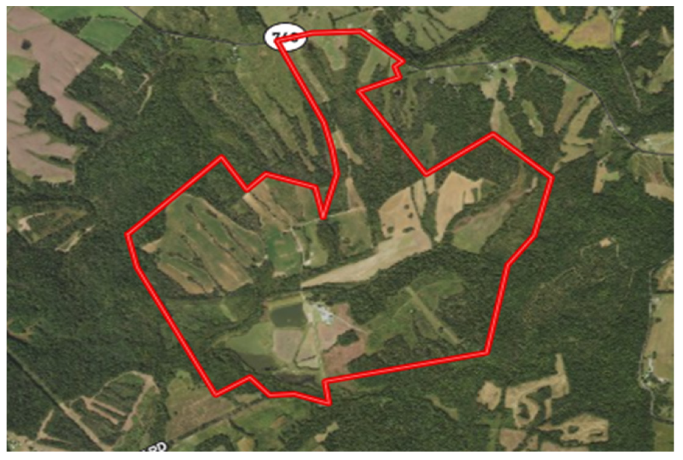
The first area was in Smithland, KY. The area receives decent solar irradiation numbers, and a large percentage of the land had been cleared for farming in the past. Trees would still need to be removed, but that would be a less intensive process there than on other properties. Unfortunately, in Kentucky property lines are far more likely to follow geographical features rather than straight boundary lines, as shown in Figure 9 of the Smithland property.
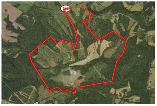
Figure 9.
Property in Smithland Kentucky [30,34].
The best course would be to sell the offshoots from the main body of the property and build on the remaining tract of land. This not only allows for a more uniform layout for the solar farm, but the sold offshoots will provide returned income, and some of the more heavily forested sections would no longer be our concern. This still leaves a sizable tract of land. Considering spacing between the rows of panels, necessary maintenance roads, and onsite buildings and infrastructure needed, there should be enough land left that a 200 MW solar farm could be installed.
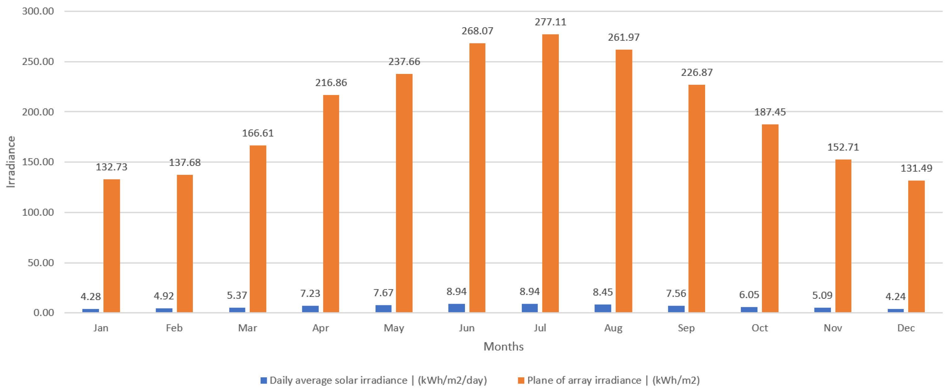
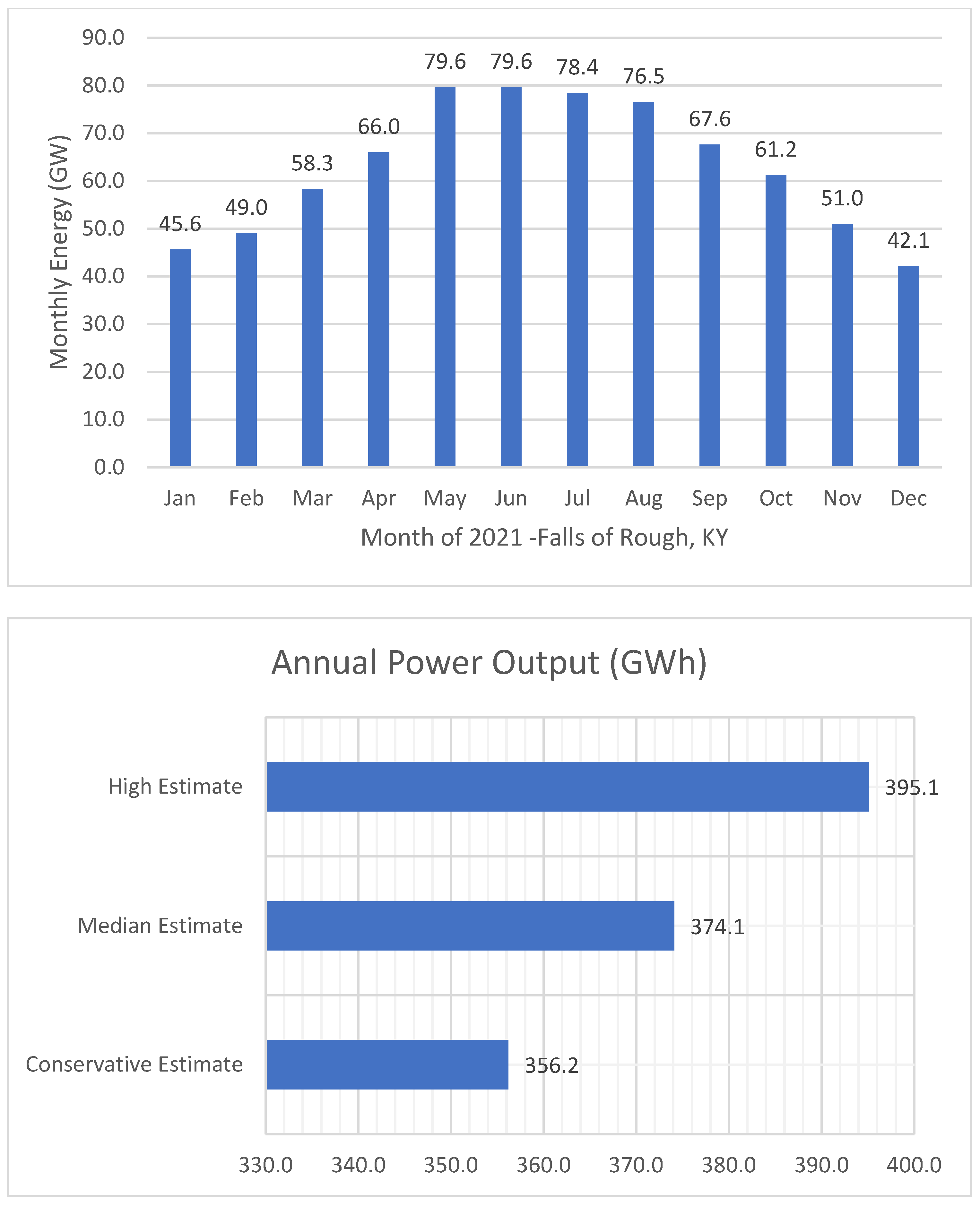
When using southern-facing standard crystalline silicon panels with a nominal efficiency of 15% on two-axis tracking, with estimated system losses of 14.93%, this leads to an output between 356.2 GWh and 395.1 GWh. The program used gives an estimate, but also specifies a range of values to be expected. Figure 10 displays the solar irradiance for the specific area as well as the plane of array irradiance (POA) which are used to quantify the incident irradiance on a given solar array. The median number presented was 374.1 GWh annually, as shown in Figure 11, which displays the annual and monthly estimates of GWh produced, and Table 3.

Figure 10.
Graph of monthly average solar irradiance and array irradiance in kWh/m2 for Smithland, KY 2021 [27].
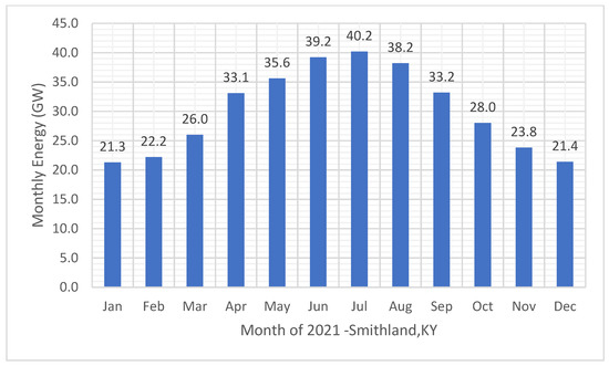
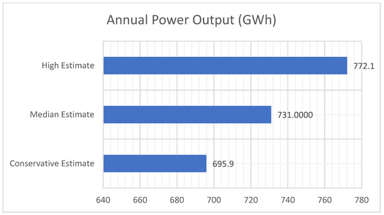
Figure 11.
Graphs of estimated GWh produced over a one-year period—2021—for potential Smithland solar farm monthly (13.1: Upper) and annually (13.2: Lower) [27,29].
Table 3.
Regarding estimates of yearly power generation by potential Smithland solar farm. Percentages are based off average annual electricity consumption in Kentucky [27,29].
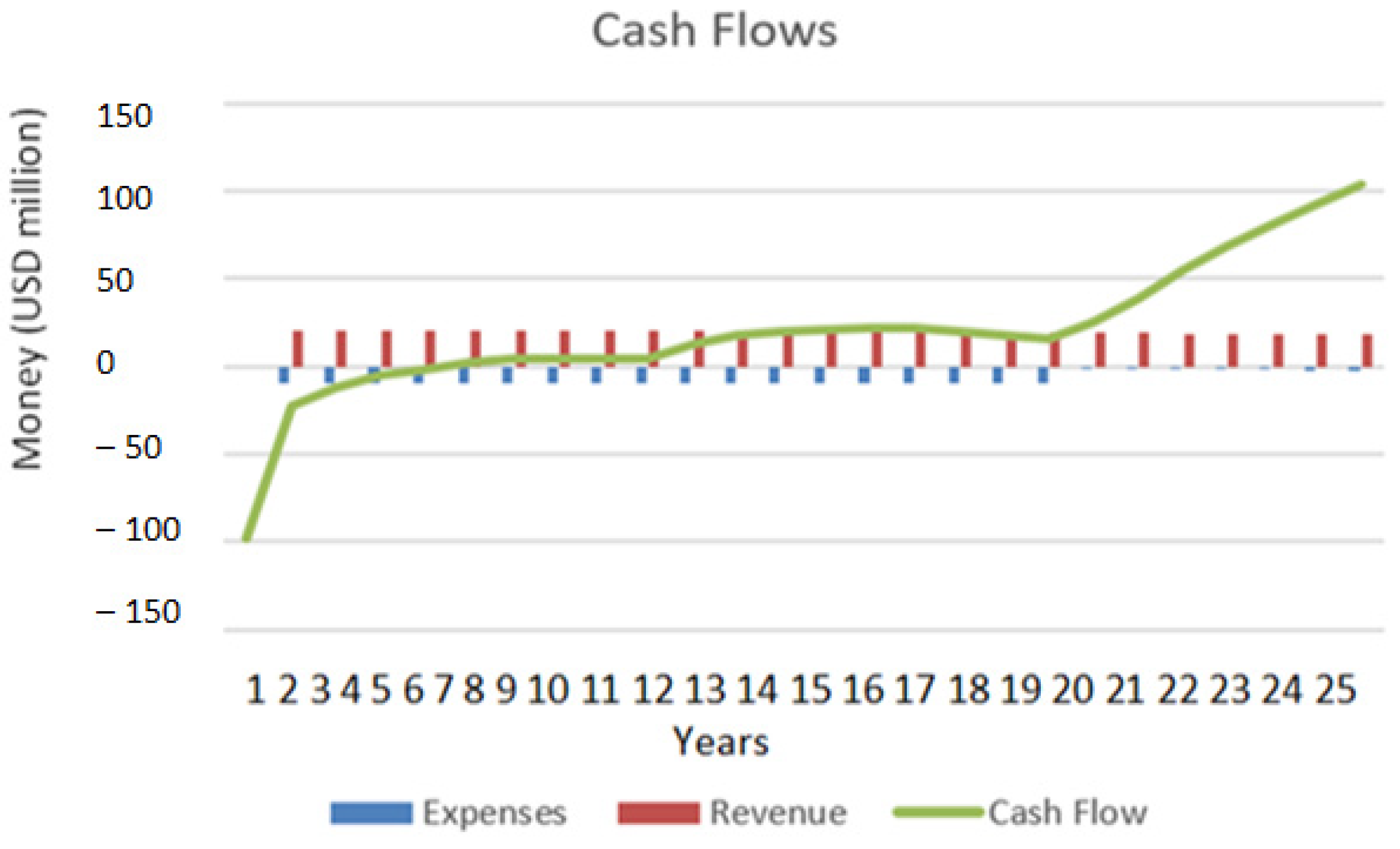
According to CREST, the final cumulative cash flow as shown in Figure 12, after the 25-year life span of the panels, was $104,094,453, and the farm became profitable in the sixth year [30].
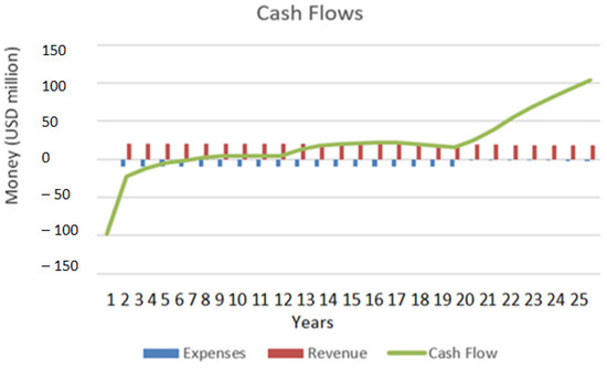
Figure 12.
Cumulative cash flow chart for Smithland solar farm [30].
3.2. Solar Farms by Location—Hickman, KY
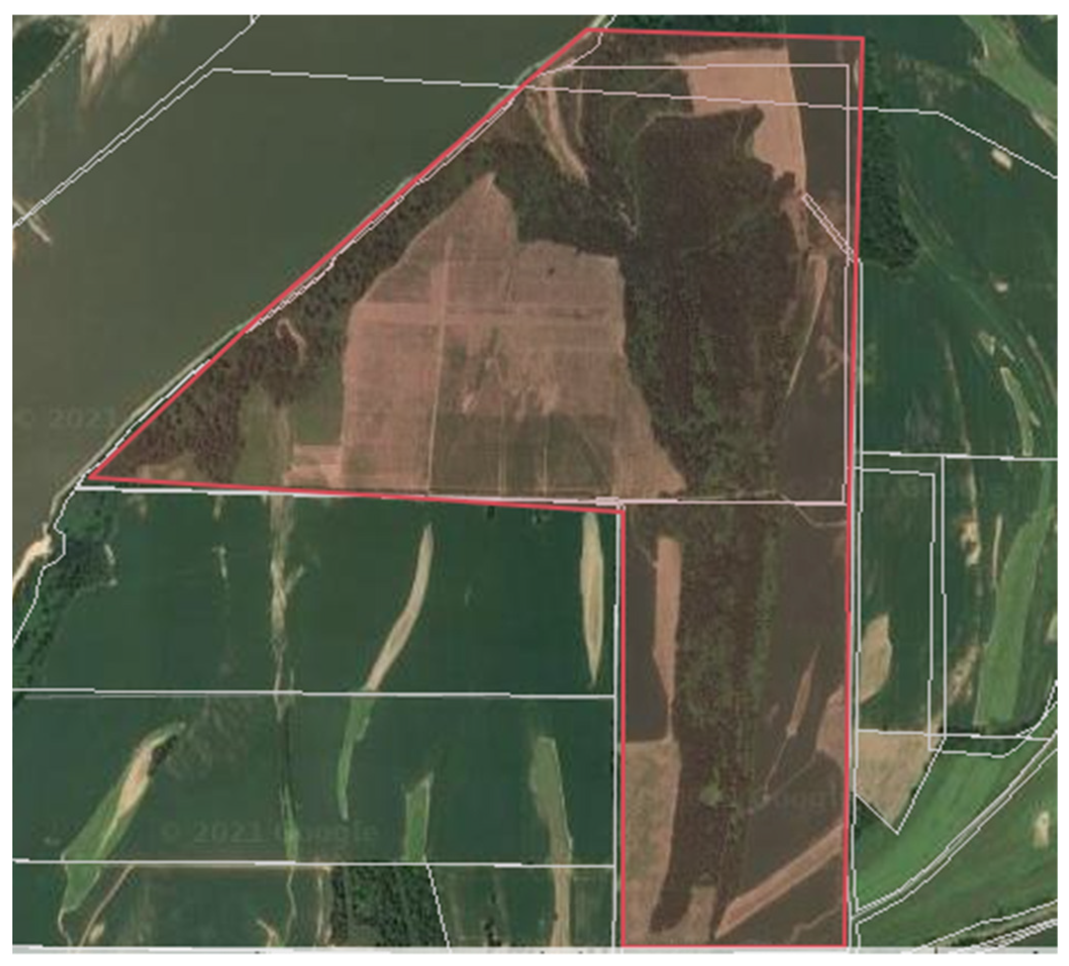
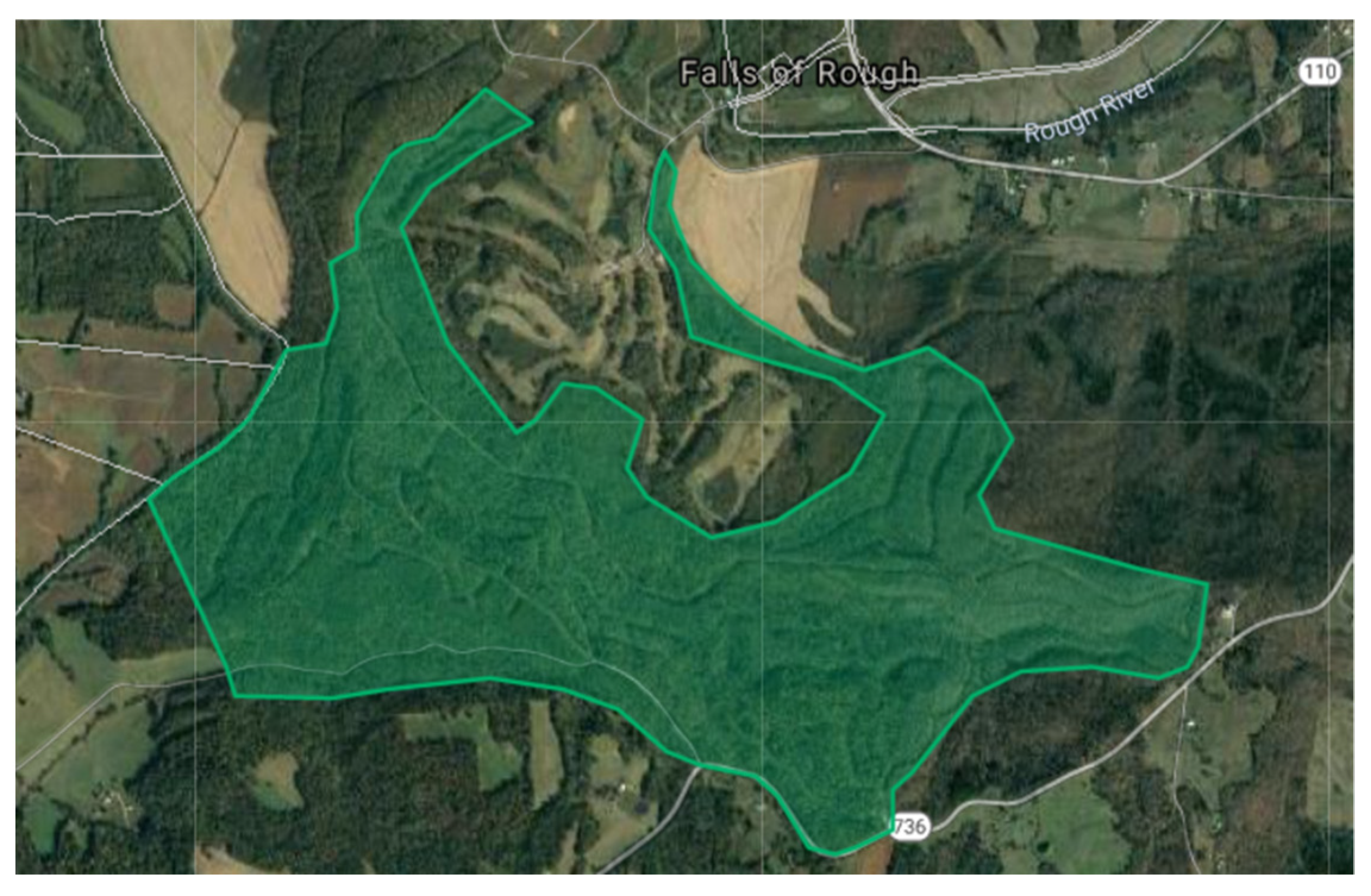
The next property was in Hickman, KY and was a larger property with cleaner borders. It was the largest property at 1036 acres shown in Figure 13, and parts of this tract of land were also used for farming and already cleared. However, there were still more trees to clear than the last property. This could be seen as either a positive or negative based on one’s outlook. Additional trees could be seen as a negative because they would take longer to clear and delay construction. However, logging is common in Kentucky, and there are many companies that will pay landowners to be able to come onto their property to log, so this could also be an additional source of income. It could help to partially fund the farm, while delegating the labor of removing trees to a third party.
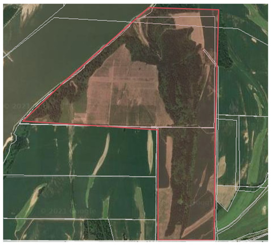
Figure 13.
Property in Hickman, KY [30,34].
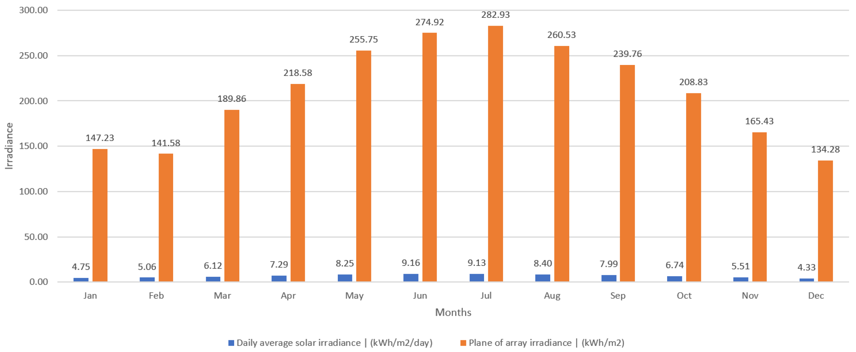
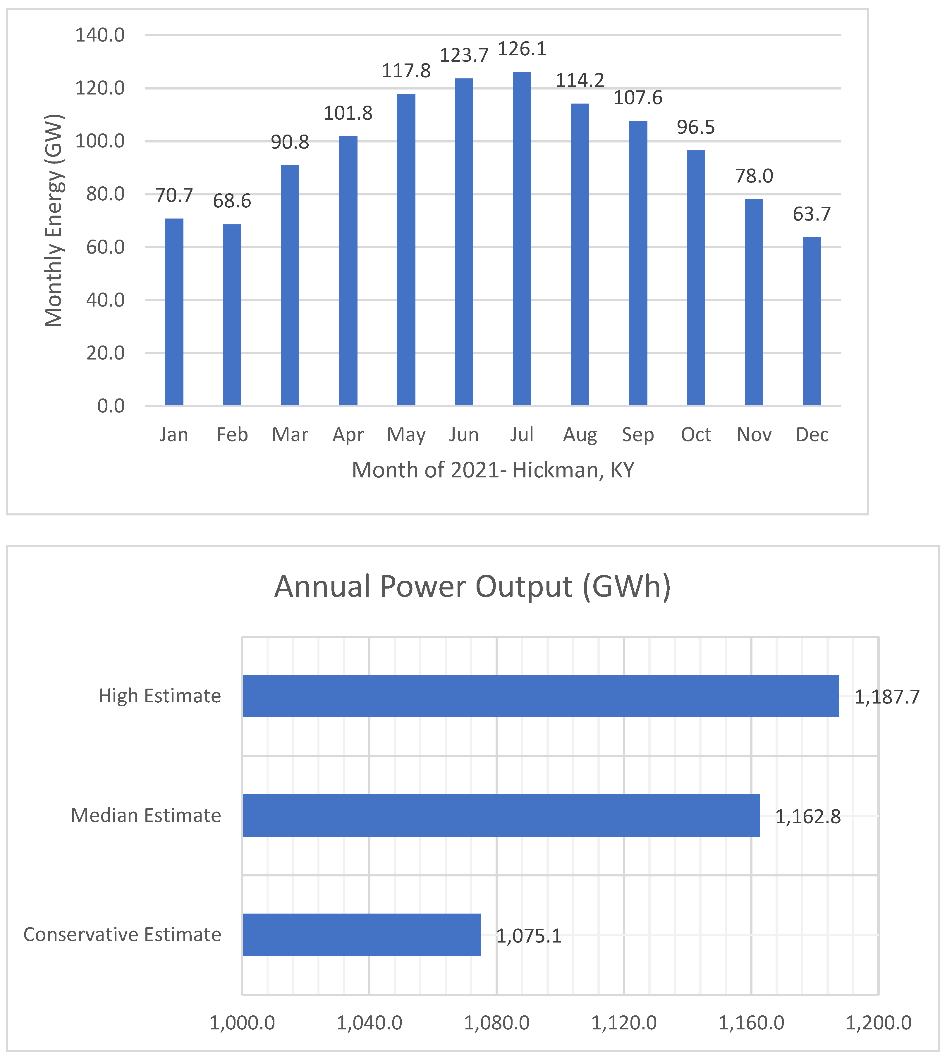
Most of the land on this property would be usable for solar panels, except for a small tract on the western end of the property. The property borders the Mississippi River, so a flood zone should be designated there to prevent flood waters from destroying solar panels. Taking these factors into account lowers the amount of usable land for solar panels. However, there is still enough to theoretically house a 600 MW solar farm. Figure 14 displays the solar irradiance for the area as well as the array irradiance. Hickman shows the largest irradiation values out of the three locations. When using the same solar setup as mentioned previously, this leads to an output between 1075.1 GWh and 1187.7 GWh, with a median value of 1162.8 GWh, as shown in Figure 15, which displays the annual and monthly estimates of GWh produced, and Table 4.
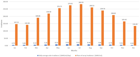
Figure 14.
Graph of monthly average solar irradiance and array irradiance in khW/m2 for Hickman, KY [27].
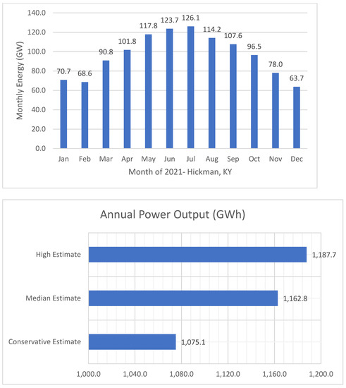
Figure 15.
Graphs of estimated GWh produced over a one-year period for potential Hickman solar farm monthly (17.1: Upper) and annually (17.2: Lower) [27,29].
Table 4.
Regarding estimates of yearly power generation by potential Hickman solar farm. Percentages are based off average annual electricity consumption in Kentucky [27,29].
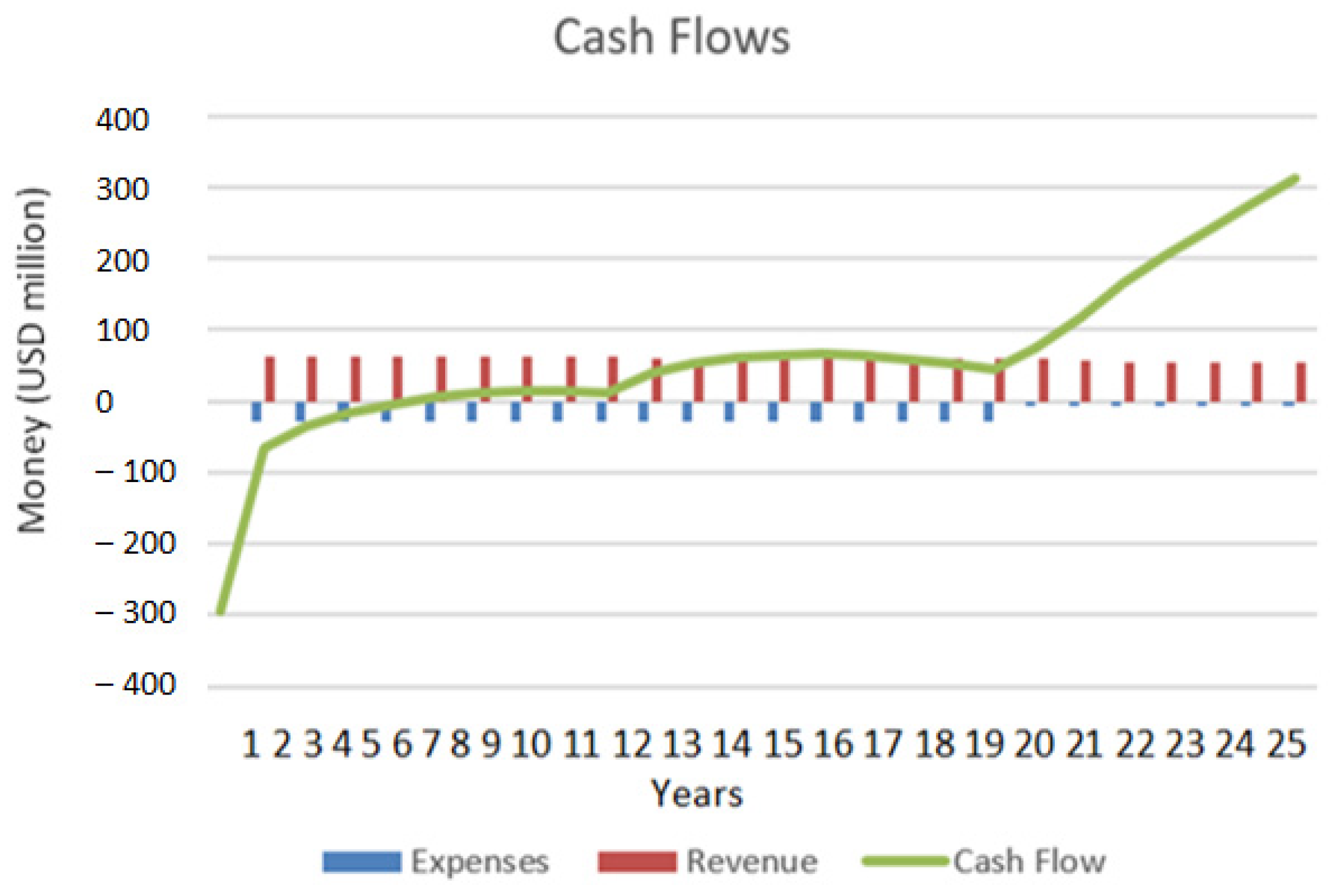
According to CREST, the final cumulative cash flow (Figure 16), after the 25-year life span of the panels, was $312,283,360, and the farm became profitable in the sixth year [30].
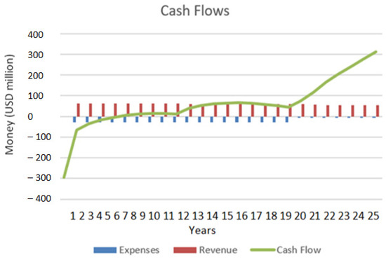
Figure 16.
Cumulative cash flow chart for Hickman solar farm [30].
3.3. Solar Farms by Location—Falls of Rough, KY
The final property was located in Falls of Rough, KY, shown in Figure 17. Despite still being a decent distance away, this location would be the closest to large population centers in Kentucky, such as Lexington and Louisville.

Figure 17.
Property in Falls of Rough, KY [30,34].
This property has 873 acres. However, this is the most heavily forested area of the three properties. This would mean an increased income for timber sold before building, but it would also mean a longer delay before construction. As with the Smithland property, there are sections of land that would be more convenient to sell. This would still leave a sizable tract of land, enough to hold a 400 MW solar farm. Figure 18 displays the solar irradiance for the area as well as the array irradiance. When using the same solar setup, this leads to an output between 696.5 GWh and 772.1 GWh, with a median value of 731.0 GWh, as shown in Figure 19, which displays the annual and monthly estimates of GWh produced, and Table 5.
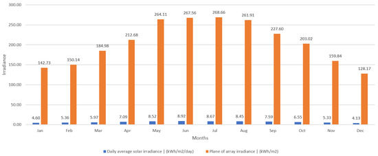
Figure 18.
Graph of monthly average solar irradiance and array irradiance in kWh/m2 for Falls of Rough, KY [27].

Figure 19.
Graphs of estimated GWh produced over a one-year period for potential Falls of Rough solar farm monthly (21.1: Upper) and annually (21.2: Lower) [27,29].
Table 5.
Regarding estimates of yearly power generation by potential Falls of Rough solar farm. Percentages are based off average annual electricity consumption in Kentucky [27,29].
According to CREST, the final cumulative cash flow (Figure 20), after the 25-year life span of the panels, was $208,188,907, and the farm became profitable in the sixth year [30].
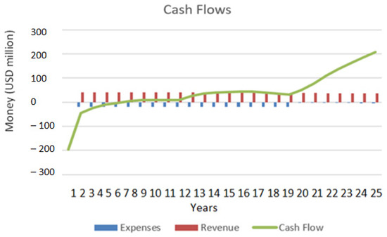
Figure 20.
Cumulative cash flow chart for Falls of Rough solar farm [30].
4. Discussion
Kentucky is one of the states which has lower than the national average for solar power generation (2.3%) [22]. To overcome this issue, first, three areas in Smithland, Hickman, and Falls of Rough were chosen based on the following factors: (1) Terrain, (2) Solar irradiance, (3) Cost and Size and (4) Proximity pre-existing infrastructure. This paper demonstrates the feasibility of large-scale solar generation in Kentucky by designing several large-scale solar farms in the state and conducting a financial analysis of these designs.
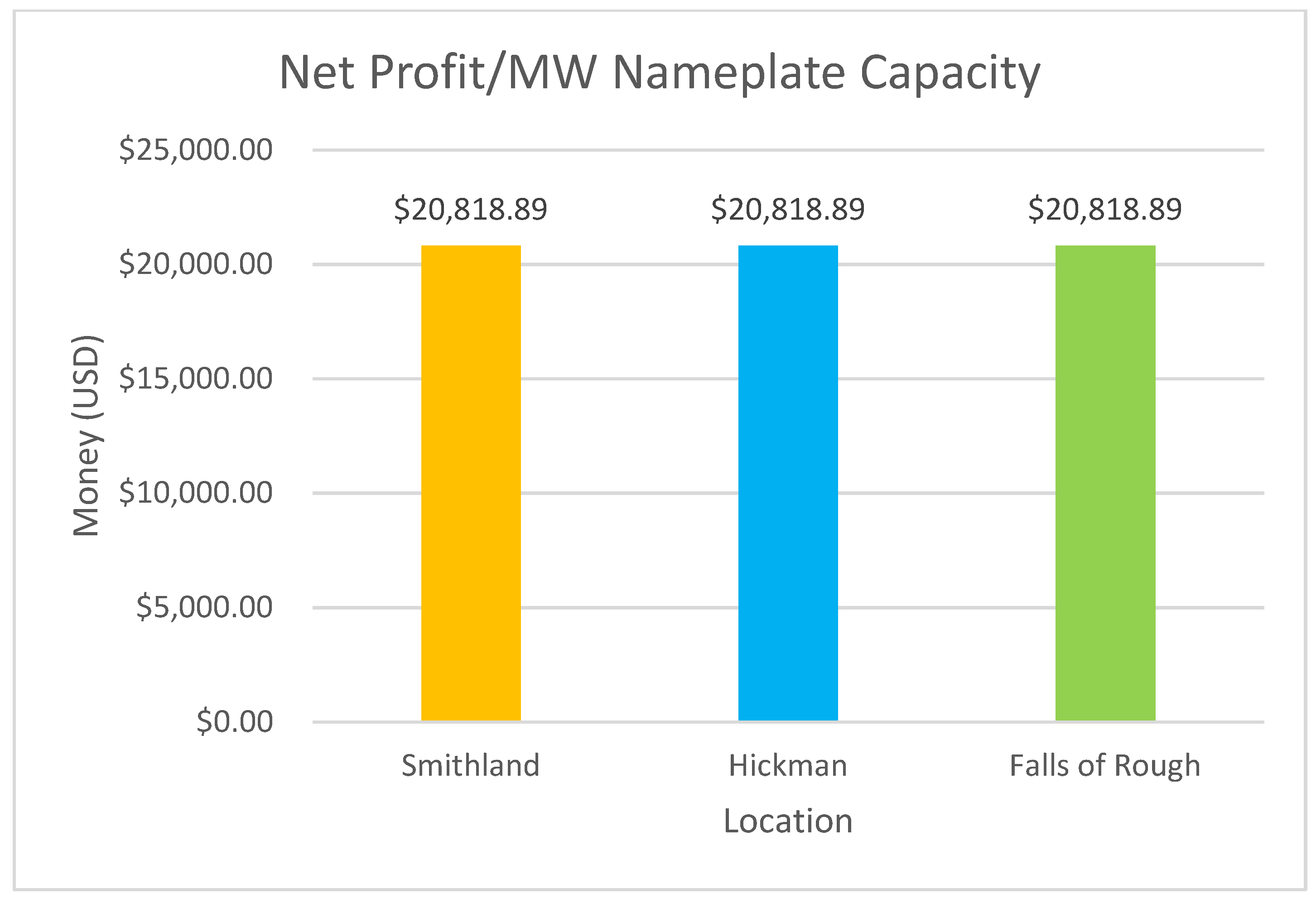
Overall, the theoretical solar panels at all three locations would total into 1.2 GW of solar panels (nameplate capacity) with an average annual power generation of 2.27 TWh. This would mean that these three plants’ theoretical generation would increase Kentucky’s annual solar electricity. This value added onto the pre-existing solar in KY would mean that 2.545% of KY’s electricity would be generated via solar. This was determined by using the average power output estimates and the power (kWh) consumed in KY in 2020. Figure 21, Figure 22 and Figure 23 are the comparison for each of the solar farms which includes power output, cumulative cash flow, average annual cash flow/nameplate capacity, and average annual cash flow/MWh. These graphs offer a comparison of the three farms and display the benefits of each location.
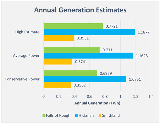
Figure 21.
Annual Power Generation Estimates [27,29].
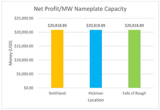
Figure 22.
Price per MW Estimates [27,28,29].

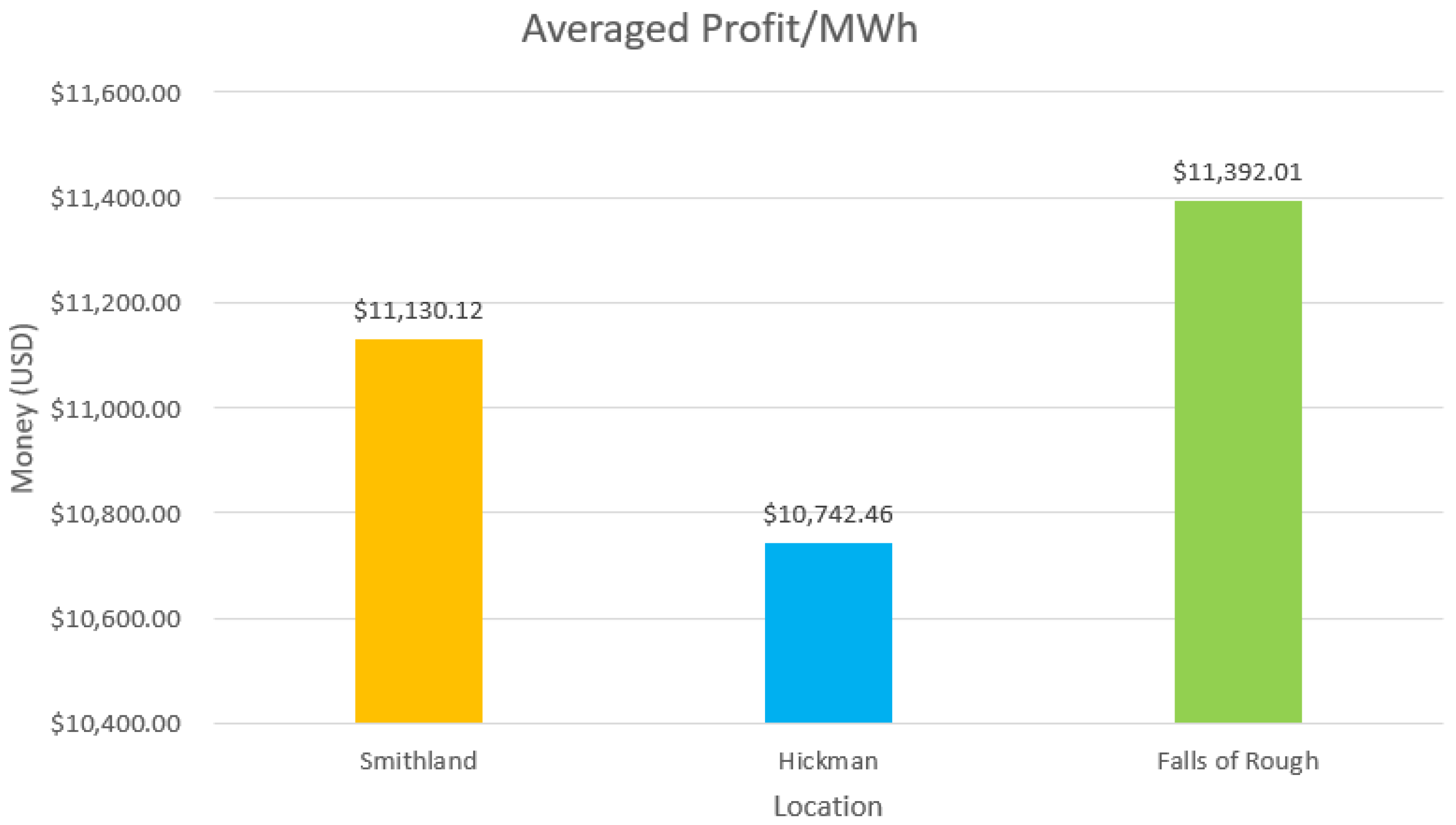
Figure 23.
Price per MWh Estimates [27,28,29].
Overall, the Hickman Farm would appear to generate the most TWh and have the largest profit. Its estimated annual power output is over 400 MWh more than Falls of Rough and just under 800 MWh more than Smithland. It also has the largest profit margin of over $312 million by the end of the solar panels lifetime. This makes sense considering it is the largest farm. However, Falls of Rough generates the most money per MWh at over $11,300 per MWh produced. Each farm has its own benefits and pitfalls, just like solar power generation has its own obstacles and advantages. Therefore, while all the farms were determined to be profitable based on the rough estimates using CREST, Hickman is the largest producer and has the largest net profit. Falls of Rough would be the most profitable percentage wise. This would seem to indicate that in Kentucky larger farms are more profitable in general. Furthermore, the more desirable location based on solar irradiation would be towards the western part of the state because both Hickman and Smithland have the higher solar irradiation values and are in the western part, whereas Falls of Rough is more centrally located. However, when considering the optimal location, there are many other factors that come into play including property taxes, land prices, etc. The location that would receive the highest percentage return after these considerations is Falls of Rough. These models prove that solar is not only feasible but could potentially be extremely profitable. They show a return on investment within 6 years, large profit margins, and annual generation of over 2.2 TWh. Solar is severely underutilized within the state—partially because of socio-economic reasons—and the belief that solar is not feasible in Kentucky is rampant. However, the data shows that creating profitable solar farms within the state is possible.
5. Conclusions
Although Kentucky has been slower to adopt solar technology in comparison to some states, the region has great potential for solar farms. The objective of this study was to analyze the economic feasibility of three potential solar farm sites within the state. Each location was analyzed based upon multiple factors including terrain, solar irradiance, cost and size, and proximity to pre-existing infrastructure.
The data collected in this study shows that solar farms in the state of Kentucky are a profitable venture worth investing in. Each of the three locations analyzed in this study show results of large profit margins, and the combined power output shows the ability to exceed the national generation percentage average of 2.3%. Even though Kentucky is one of the states which is currently below the national average for solar energy production, this study proves that the state contains great potential for solar farms. If the state begins investing in and profiting from solar energy production, Kentucky could be the state that helps bring forth a paradigm shift as it relates to renewable energy throughout Appalachia.
Author Contributions
Conceptualization, Y.K. and A.S.; software, A.S.; validation, Y.K. and A.S.; investigation, A.S.; writing—original draft preparation, A.S. and Y.K.; writing—review and editing, A.S., Y.K. and J.F.; visualization, A.S. and Y.K.; supervision, Y.K. and J.F.; project administration, Y.K. and A.S.; All authors have read and agreed to the published version of the manuscript.
Funding
This research received no external funding.
Institutional Review Board Statement
Not applicable.
Informed Consent Statement
Not applicable.
Data Availability Statement
Not available.
Conflicts of Interest
The authors declare no conflict of interest.
Appendix A
Table A1.
CREST Financial Inputs [28].
Table A1.
CREST Financial Inputs [28].
| Category | Input | Description |
|---|---|---|
| Technology | Photovoltaic | Type of solar technology being used |
| Generator Nameplate Capacity | Varies on Location | Assumed system capacity |
| Net Capacity Factor | State Average | the options here are to enter a custom factor or to select State Average |
| State | KY | If State Average is chosen, enter the state here |
| Annual Production Degradation | 0.50% | Annual percentage the system has degraded. The value used was based on typical degradation for the panels used |
| Project Useful Life | 25 | How long the panels are expected to last before needing replacement |
| Total Installed Cost | Varies on Location | Total costs for standard operation, maintenance, etc. in $(USD)/Watt DC. This was based on averages for solar farms of similar size in areas with similar income |
| Fixed O & M Expense, Yr 1 | $6.50/kW-yr dc | Total expected fixed costs |
| O & M Cost Inflation, Initial Period | 1.60% | Inflation rate 1 will last over a set initial period |
| Initial Period Ends Last Day Of: | 10 | The time period over which inflation rate 1 lasts |
| O & M Cost Inflation, thereafter | 1.60% | Inflation Rate after the initial period ends |
| % Debt | 45% | Theoretical amount of funds borrowed |
| Debt Term | 18 | number of years for debt repayment |
| Interest Rate on Term Debt | 7% | interest rate set by lender |
| Lender’s Fee | 3% | one-time fee collected by the lender |
| DSCR | 1.2–1.45% | Debt Service Coverage Ratio is yearly cash flow/(annual principal + interest) |
| Target After-Tax Equity IRR | 12% | minimum rate of return |
| Other Closing Costs | 0% | any additional costs |
| Is the owner a taxable entity? | Yes | |
| Federal Income Tax Rate | 35% | |
| Federal Tax Benefits used as generated or carried forward? | Generated | determines whether deprecation is monetized as it occurs or after the project has sufficient tax liability |
| State Income Tax Rate | 0% | |
| State Tax Benefits used as generated or carried forward? | Generated | determines whether deprecation is monetized as it occurs or after the project has sufficient tax liability |
| Payment Duration for Cost-Based Tariff | FIT Contract length—determined by policymakers | |
| % Of Year 1 Tariff Escalated | portion of tariff that can be escalated | |
| Cost-Based Tariff Escalation Rate | used to account for levelized nominal tariff rate | |
| Federal Incentives | Cost-Based | |
| Investment Tax Credit (ITC) or Cash Grant? | ITC | |
| ITC Amount | 22% | |
| ITC Utilization Factor | 100% | How much of the project expenses the ITC can be applied to |
| Additional Federal Grants | 0 | |
| Federal Grants Treated as Taxable Income? | No | |
| State Rebates/Grants | No | |
| $ Cap on State Rebates/Grants | $500,000 | Maximum amount of state grants or rebates a project can legally accept |
| State Grants Treated as Taxable Income? | No | |
| 1st Equipment Replacement | 10 | Year equipment will need maintenance/replacement |
| 1st Replacement Cost ($ in year replaced) | $0.24 | |
| 2nd Equipment Replacement | 20 | Year equipment will need 2nd maintenance/replacement |
| 2nd Replacement Cost ($ in year replaced) | $0.24 | |
| Number of months of Debt Service | 6 | lenders often require a debt service amount set aside equal to x amount of months’ repayment |
| Number of months of O&M Expense | 6 | how many months of O & M should be set aside in a reserve account |
| Interest on All Reserves | 2% |
Table A2.
CREST Example [28].
Table A2.
CREST Example [28].
| Project Size and Performance | Units | Input Value |
|---|---|---|
| Generator Nameplate Capacity | kW dc | 400,000 |
| Net Capacity Factor: Select “State Average” or “Custom” → | State Average | |
| Net C.F.: If “State Average” method, then select state → | KY | |
| Net Capacity Factor, Yr 1 | 14.0% | |
| Production, Yr 1 | kWh | 490,669,792 |
| Annual Production Degradation | % | 0.5% |
| Project Useful Life | years | 25 |
| Capital Costs | Units | Input Value |
| Select Cost Level of Detail | Simple | |
| Total Installed Cost | $/Watt dc | $0.89 |
| Total Installed Cost (before rebates/grants, if any) | $ | $356,000,000 |
| Total Installed Cost (before rebates/grants, if any) | $/Watt dc | $0.89 |
| Operations & Maintenance | Units | Input Value |
| Select Cost Level of Detail | Simple | |
| Fixed O&M Expense, Yr 1 | $/kW-yr dc | $6.50 |
| Variable O&M Expense, Yr 1 | ¢/kWh | 0.00 |
| O&M Cost Inflation, initial period | % | 1.6% |
| Initial Period ends last day of: | year | 10 |
| O&M Cost Inflation, thereafter | % | 1.6% |
| Permanent Financing | Units | Input Value |
| % Debt (% of hard costs) (mortgage-style amort.) | % | 45% |
| Debt Term | years | 18 |
| Interest Rate on Term Debt | % | 7.00% |
| Lender’s Fee (% of total borrowing) | % | 3.0% |
| Required Minimum Annual DSCR | 1.20 | |
| Actual Minimum DSCR, occurs in → | Year 18 | 1.60 |
| Minimum DSCR Check Cell (If “Fail”, read note ==>) | Pass/Fail | Pass |
| Required Average DSCR | 1.45 | |
| Actual Average DSCR | 1.73 | |
| Average DSCR Check Cell (If “Fail”, read note ==>) | Pass/Fail | Pass |
| % Equity (% hard costs) (soft costs also equity funded) | % | 55% |
| Target After-Tax Equity IRR | % | 12.00% |
| Weighted Average Cost of Capital (WACC) | % | 8.47% |
| Other Closing Costs | $ | $0 |
| Summary of Sources of Funding for Total Installed Cost | ||
| Senior Debt (funds portion of hard costs) | 45% | $160,200,000 |
| Equity (funds balance of hard costs + all soft costs) | 55% | $195,800,000 |
| Total Value of Grants (excl. pmt in lieu of ITC, if applicable) | 0% | $0 |
| Total Installed Cost | $ | $356,000,000 |
| Tax | Units | Input Value |
| Is owner a taxable entity? | Yes | |
| Federal Income Tax Rate | % | 35.0% |
| Federal Tax Benefits used as generated or carried forward? | As Generated | |
| State Income Tax Rate | % | 8.5% |
| State Tax Benefits used as generated or carried forward? | As Generated | |
| Effective Income Tax Rate | % | 40.53% |
| Depreciation Allocation | see table ==> | |
| Cost-Based Tariff Rate Structure | Units | Input Value |
| Payment Duration for Cost-Based Tariff | years | 25 |
| % of Year-One Tariff Rate Escalated | % | 0.0% |
| Cost-Based Tariff Escalation Rate | % | 0.0% |
| Forecasted Market Value of Production; applies after Incentive Expiration | ||
| Select Market Value Forecast Methodology | Year One | |
| Value of energy, capacity & RECs, Yr 1 | ¢/kWh | 5.00 |
| Market Value Escalation Rate | % | 3.0% |
| Federal Incentives | Units | Input Value |
| Select Form of Federal Incentive | Cost-Based | |
| Investment Tax Credit (ITC) or Cash Grant? | ITC | |
| ITC or Cash Grant Amount | % | 22% |
| ITC utilization factor, if applicable | % | 100% |
| ITC or Cash Grant | $ | $73,620,800 |
| Is PBI Tax-Based (PTC) or Cash-Based (REPI)? | Tax Credit | |
| PBI Rate | ¢/kWh | 2.30 |
| PBI Utilization or Availability Factor, if applicable | % | 100.0% |
| PBI Duration | yrs | 10 |
| PBI Escalation Rate | % | 2.0% |
| Additional Federal Grants (Other than Section 1603) | $ | $0 |
| Federal Grants Treated as Taxable Income? | No | |
| State Rebates, Tax Credits and/or REC Revenue | Units | Input Value |
| Select Form of State Incentive | Neither | |
| ITC Amount | % | 30% |
| Utilization Factor, if applicable | % | 100% |
| State ITC realization period | yrs | 5 |
| Total State ITC, over realization period | $ | $0 |
| Is Performance-Based Incentive Tax Credit or Cash Pmt? | Cash | |
| Annual $ Cap on Performance-Based Incentive | $ | $0 |
| If cash, is state PBI or REC taxable? | Yes | |
| PBI or REC Rate | ¢/kWh | 1.50 |
| PBI Utilization Factor, if applicable | % | 100.0% |
| PBI or REC Payment Duration | yrs | 10 |
| PBI or REC Escalation Rate (pos. or neg.) | % | 2.0% |
| Additional State Rebates/Grants | $/Watt | $0.00 |
| Total $ Cap on State Rebates/Grants | $ | $500,000 |
| State Rebates/Grants Treated as Taxable Income? | No | |
| Capital Expenditures During Operations: Inverter Replacement | Input Value | |
| 1st Equipment Replacement | year | 10 |
| 1st Replacement Cost ($ in year replaced) | $/Watt dc | $0.235 |
| 2nd Equipment Replacement | year | 20 |
| 2nd Replacement Cost ($ in year replaced) | $/Watt dc | $0.235 |
| Reserves Funded from Operations | Units | Input Value |
| Decommissioning Reserve | ||
| Fund from Operations or Salvage Value? | Operations | |
| Reserve Requirement | $ | $0 |
| Initial Funding of Reserve Accounts | Units | Input Value |
| Debt Service Reserve | ||
| # of months of Debt Service | months | 6 |
| Initial Debt Service Reserve | $ | $7,962,949 |
| O&M Reserve/Working Capital | ||
| # of months of O&M Expense | months | 6 |
| Initial O&M and WC Reserve | $ | $1,583,103 |
| Interest on All Reserves | % | 2.0% |
| Depreciation Allocation | Input Values | |
| Bonus Depreciation | Yes | |
| % of Bonus Depreciation applied in Year 1 | 50% | |
| Allocation of Costs | 5-year MACRS | 7-year MACRS |
| Total Installed Cost | 94.0% | 0.0% |
References
- NREL. Solar Resource Data, Tools, and Maps. NREL.gov. Available online: https://www.nrel.gov/gis/solar.html (accessed on 15 December 2021).
- McDonald, A.; Bills, J. Appalachia-Science in the Public Interest and the Kentucky Solar Partnership. In The Kentucky Solar Energy Guide; 2005. [Google Scholar]
- Johnson, J.A. Analysis of Photovoltaic Energy in the Eastern Kentucky Region and the Residential Financial Feasibility. Ph.D. Thesis, Morehead State University, Morehead, KY, USA, 2018. [Google Scholar]
- Michaud, G. Perspectives on community solar policy adoption across the United States. Renew. Energy Focus 2020, 33, 1–15. [Google Scholar] [CrossRef]
- Gagnon, P.; Das, P. Projections of Distributed Photovoltaic Adoption in Kentucky through 2040 (No. NREL/PR-6A20-68656); National Renewable Energy Lab. (NREL): Golden, CO, USA, 2017. [Google Scholar] [CrossRef]
- Solar Energy Industries Association. Kentucky Solar. Available online: https://www.seia.org/state-solar-policy/kentucky-solar (accessed on 20 June 2022).
- Hale, B.; Kramer, S.W. Installation of Solar Panels in a Residential Setting: A Feasibility Study for a Southern US City. Available online: https://2015.creative-construction-conference.com/CCC2015_proceedings/CCC2015_69_Hale.pdf (accessed on 20 June 2022).
- EIA. U.S. Energy Information Administration-EIA-Independent Statistics and Analysis. Kentucky-State Energy Profile Analysis-U.S. Energy Information Administration (EIA). 15 July 2022. Available online: https://www.eia.gov/state/analysis.php?sid=KY#89 (accessed on 22 October 2021).
- Kentucky Office of Energy Policy and Kentucky Geological Survey. Kentucky Energy Infrastructure. 14 December 2021. Available online: https://kgs.uky.edu/kgsmap/kyenergy/viewer.asp (accessed on 15 December 2021).
- Amburgey, B.H. The Politics of Unionization: The Impact of Politics on the Strength of Kentucky Coal Miners’ Unions. 2020. Available online: https://ir.library.louisville.edu/honors/210/ (accessed on 20 June 2022).
- Net Metering. DSIRE. Available online: https://programs.dsireusa.org/system/program/detail/1081 (accessed on 31 May 2021).
- Noll, D.; Dawes, C.; Rai, V. Solar community organizations and active peer effects in the adoption of residential PV. Energy Policy 2014, 67, 330–343. [Google Scholar] [CrossRef]
- Kentucky Touchstone’s Energy Cooperative. Green Benefits. Envirowatts. 12 March 2021. Available online: https://www.envirowattsky.com/green-benefits/ (accessed on 31 May 2020).
- NC Clean Energy Technology Center. Programs. DSIRE. 27 August 2021. Available online: https://programs.dsireusa.org/system/program/ky/solar (accessed on 15 December 2021).
- East Kentucky Power Corporation. About Cooperative Solar. Cooperative Solar. Available online: https://www.cooperativesolar.com/about (accessed on 22 October 2021).
- Energy, D. Duke Energy unveils plans for its first solar power plants in Kentucky. Duke Energy | News Center. 14 July 2017. Available online: https://news.duke-energy.com/releases/duke-energy-unveils-plans-for-its-first-solar-power-plants-in-kentucky (accessed on 15 December 2021).
- Mayhew, C. Duke Energy Opens Solar Power Farms Near Walton. The Enquirer. 27 April 2018. Available online: https://www.cincinnati.com/story/news/local/kentoncounty/2018/04/24/duke-energy-opens-kentucky-solar-power-plant/546589002/ (accessed on 15 December 2021).
- EIA. EIA electricity Data Now Include Estimated Small-Scale Solar PV Capacity and Generation. Homepage-U.S. Energy Information Administration (EIA). Available online: https://www.eia.gov/todayinenergy/detail.php?id=23972 (accessed on 31 May 2022).
- Hiatt, R.S.; Parker, B.F. Solar Energy for Heating Farm Structures in Kentucky. 1979. Available online: https://uknowledge.uky.edu/aeu_reports/71/ (accessed on 20 June 2022).
- Duke, H. Encouraging rooftop solar: What policy is right for Kentucky? N. Ky. L. Rev. 2020, 47, 155. [Google Scholar]
- Kentucky Solar Energy Society. Solar Stories Map. 2020. Available online: https://www.kyses.org/SolarStories-Map (accessed on 20 June 2022).
- Savion Energy. Martin County Solar Project to Advance–Savion’s First Solar Project on a Reclaimed Coal Mine. SavionEnergy. 9 December 2021. Available online: https://savionenergy.com/martin-county-solar-project-to-advance-savions-first-solar-project-on-a-reclaimed-coal-mine/ (accessed on 28 September 2022).
- Salasovich, J.; Geiger, J.; Mosey, G.; Healey, V. Feasibility Study of Economics and Performance of Solar Photovoltaics at the Price Landfill Site in Pleasantville, New Jersey. A Study Prepared in Partnership with the Environmental Protection Agency for the RE-Powering America’s Land Initiative: Siting Renewable Energy on Potentially Contaminated Land and Mine Sites (No. NREL/TP-7A40-58480); National Renewable Energy Lab. (NREL): Golden, CO, USA, 2013. [Google Scholar]
- Jo, J.H.; Ilves, K.; Barth, T.; Leszczynski, E. Implementation of a large-scale solar photovoltaic system at a higher education institution in Illinois, USA. AIMS Energy 2017, 51, 54–62. [Google Scholar] [CrossRef]
- EIA. U.S. Energy Information Administration-EIA-Independent Statistics and Analysis. Electricity in the U.S.-U.S. Energy Information Administration (EIA). 18 March 2021. Available online: https://www.eia.gov/energyexplained/electricity/electricity-in-the-us.php (accessed on 22 October 2021).
- WorldAtlas. Kentucky Maps & Facts. WorldAtlas. 9 January 2022. Available online: https://www.worldatlas.com/maps/united-states/kentucky (accessed on 30 June 2022).
- PVWatts [Computer Software]. 2022. Available online: https://pvwatts.nrel.gov/version_6_3.php (accessed on 20 June 2022).
- CREST: Cost of Renewable Energy Spreadsheet Tool [Computer Software]. 2010. Available online: https://www.nrel.gov/analysis/crest.html (accessed on 20 June 2022).
- SAM: System Advisor Model. [Computer Software]. 2021. Available online: https://sam.nrel.gov/download.html (accessed on 20 June 2022).
- Kentucky Land for Sale over 500 Acres. LandWatch. (n.d.). Available online: https://www.landwatch.com/kentucky-land-for-sale/acres-over-500 (accessed on 15 December 2021).
- Gauli, U. Feasibility Study on A Large Scale Solar PV System. 2016. Available online: https://www.theseus.fi/bitstream/handle/10024/112804/Gauli_Umesh.pdf?sequence=1 (accessed on 20 June 2022).
- NREL, 2018; Global Horizontal Solar Irradiance: National Solar Irradiation Database Physical Solar Model. NREL: Solar Resource Maps. Available online: https://www.nrel.gov/gis/assets/images/solar-annual-ghi-2018-usa-scale-01.jpg (accessed on 28 September 2022).
- Gilman, P.; Dobos, A.; DiOrio, N.; Freeman, J.; Janzou, S.; Ryberg, D. SAM Photovoltaic Model Technical Reference Update; NREL: Golden, CO, USA, 2018.
- Google Maps. 2021. Available online: https://www.google.com/maps (accessed on 20 June 2022).


Publisher’s Note: MDPI stays neutral with regard to jurisdictional claims in published maps and institutional affiliations. |
© 2022 by the authors. Licensee MDPI, Basel, Switzerland. This article is an open access article distributed under the terms and conditions of the Creative Commons Attribution (CC BY) license (https://creativecommons.org/licenses/by/4.0/).