Article

Hydrodynamic Effects of Mastigonemes in the Cryptophyte Chilomonas paramecium

1
Department of Mechanical Engineering, University of Utah, Salt Lake City, UT 84112, USA
2
Core Research Facilities, Health Science, University of Utah, Salt Lake City, UT 84112, USA
3
School of Biological Sciences, University of Utah, Salt Lake City, UT 84112, USA
*
Authors to whom correspondence should be addressed.
Hydrobiology 2024, 3(3), 159-182; https://doi.org/10.3390/hydrobiology3030012
Submission received: 31 May 2024 / Revised: 2 July 2024 / Accepted: 10 July 2024 / Published: 17 July 2024

Abstract

:
Many swimming protists travel by actuating whip-like flagella to generate thrust. While many organisms’ flagella have been observed to have hair-like protrusions called mastigonemes, the function of these mastigonemes is not known. In particular, however, although theory, numerics, and some experiments suggest that mastigonemes can initiate the reversal in direction of thrust generated relative to the direction of traveling waves propagated along flagella, other experiments have found that they do not have hydrodynamic effects. Thus, it remains unclear whether mastigonemes have a hydrodynamic effect and function; additionally, any hydrodynamic effects may be species-dependent, which calls for the investigation of additional species. In this work, we report experimental observations of the cryptophyte C. paramecium that obtain their cell body, flagellar, and mastigoneme geometries, as well as their swimming kinematics and behavior. We then use the observed geometries and kinematics to numerically simulate swimming trajectories for a particularly well-characterized reorientation event, with and without various configurations of the mastigonemes. The comparison of numerical and experimental results shows that a configuration of mastigonemes in the beating plane best reproduces the observed reorientation dynamics, suggesting that in C. paramecium, although mastigonemes do not lead to gross changes in motility, such as thrust reversal, they do exert important quantitative effects.

1. Introduction

Protists are predominantly unicellular eukaryotic organisms that inhabit a wide range of habitats and exhibit a variety of shapes and forms. Many swimming protists actuate whip-like appendages called flagella in order to generate the required thrust to explore their environment [1]. Common flagellated protists include cryptophytes (also called cryptomonads), a delineated protist phylum. These biflagellated protists are nanoplankton (2.0–20 μm in size) and are ubiquitous [2,3,4,5,6,7,8,9]. They are notably present in cold, deep, or relatively dark environments [10,11,12] throughout the year and are often reported as one of the most prominent or even dominant algal groups at certain times of the year [9]. Cryptophytes are significant contributors to aquatic food chains as nutrient-rich [13], nontoxic prey for planktonic ciliate, dinoflagellate, or copepod predators [9,14,15,16,17]. Their photosynthetic forms are major phototrophic components in marine planktonic communities, with wide distributions from coastal to oceanic waters in the tropical, temperate, and polar regions [18,19,20,21,22,23,24,25].
There is considerable interest in understanding the functional differences between different types of flagella, particularly regarding variations in length, structure, and mechanosensing abilities. For instance, studies have shown that long flagella can generate more thrust compared to short flagella [26], and eukaryotic flagella differ significantly from prokaryotic flagella in terms of structure and function [26,27]. Additionally, smooth flagella and those displaying hairs called “mastigonemes” exhibit different swimming dynamics and mechanosensing capabilities [28,29]. These studies indicate that flagellar morphology can influence swimming speed and navigation abilities, which are crucial for survival in diverse aquatic environments.
One of the striking attributes of the cryptophyte locomotion system lies in the presence of thin rigid or tubular hairs on the surface of their unequally sized whipping flagella. These hairs are fibrous ultrastructures of nanometer-scale thickness. The nature and arrangement of flagellar appendages in cryptophytes are quite diverse [30,31,32]. While the taxonomic significance of the flagellar hairs is not entirely clear, some genera show characteristic patterns [31,33,34]. The species of the Chilomonas genus display one row of mastigonemes on each flagellum. The role of these flagellar structures is currently unknown, but according to theoretical and numerical approaches, mastigonemes can induce a reversal of the swimming direction relative to the wave propagation along the flagellum [28,35,36,37]: a smooth flagellum generates thrust in the direction of wave propagation, but a flagellum with mastigonemes generates thrust in the opposite direction. It has been demonstrated that the effects of the antibody-induced disruption of mastigoneme arrangement in zoosporic fungi strongly alter the swimming behavior and beating pattern of the cells, supporting the hypothesis that tubular mastigonemes are responsible for thrust reversal [36]. Conversely, recent experimental studies highlighted the lack of hydrodynamic contributions from the flagellar hairs of the model organism Chlamydomonas reinhardtii, a biflagellate chlorophyte protist [38]. However, it should be noted that C. reinhardtii bears flimsier mastigonemes than the hairs found in cryptophytes. From this discrepancy arises the question of whether or not mastigonemes have a hydrodynamic effect in cryptophytes. Since the distribution of mastigonemes is species-dependent, perhaps their hydrodynamic effects could be caused by the evolutionary selection of these appendages in cryptophytes. The potential hydrodynamic benefits from mastigonemes could enhance the competitive ability of the cells, a major factor contributing to shaping the trophic niches of different species.
In this work, we study the mastigoneme geometry and configuration of Chilomonas paramecium through electron microscopy using stationary fixed cells and perform phase contrast microscopy to observe the trajectories and kinematics of the cells during swimming. We also numerically simulate the trajectories of C. paramecium using the structural characteristics of the cell body, flagella, and mastigonemes determined from electron microscopy, together with the flagellar waveforms relative to the cell body extracted from microscopy videos, as input. In order to determine whether mastigonemes influence the hydrodynamics of the cell, we focus on a reorientation event spotted using phase contrast microscopy, which fortuitously showed both flagella beating in 2D within the field of view. We compare the observed reorientation and displacement of the cell to the results of numerical simulations, with and without mastigonemes. In the simulations, mastigonemes affect the amount of reorientation and displacement of the cell, and simulations with a specific configuration of mastigonemes most closely matches observations, suggesting that they do have a hydrodynamic effect for C. paramecium.

2. Methods

2.1. Choice and Cultivation of the Cryptophyte Species

We chose the cryptophyte Chilomonas paramecium as a model organism in our research work because it is easy to cultivate and maintain in the laboratory. Furthermore, it is a simple species to obtain, as it is commonly used for demonstrating flagellate motility and presenting protists in schools. Chilomonas is a colorless cryptophyte genus that includes approximately 25 species, whose nutrition appears to be entirely osmotrophic [30]. This genus is mainly known by widely reported C. paramecium that inhabits mostly freshwater environments, although there have been some reported sightings in estuarine and marine habitats [30,39,40,41]. Cultures of C. paramecium were obtained from Carolina Biological Supply Co., Ltd. (Burlington, NC, USA). They were grown with the addition of a sterilized wheat seed at 20 °C for 5 to 10 days before observation.

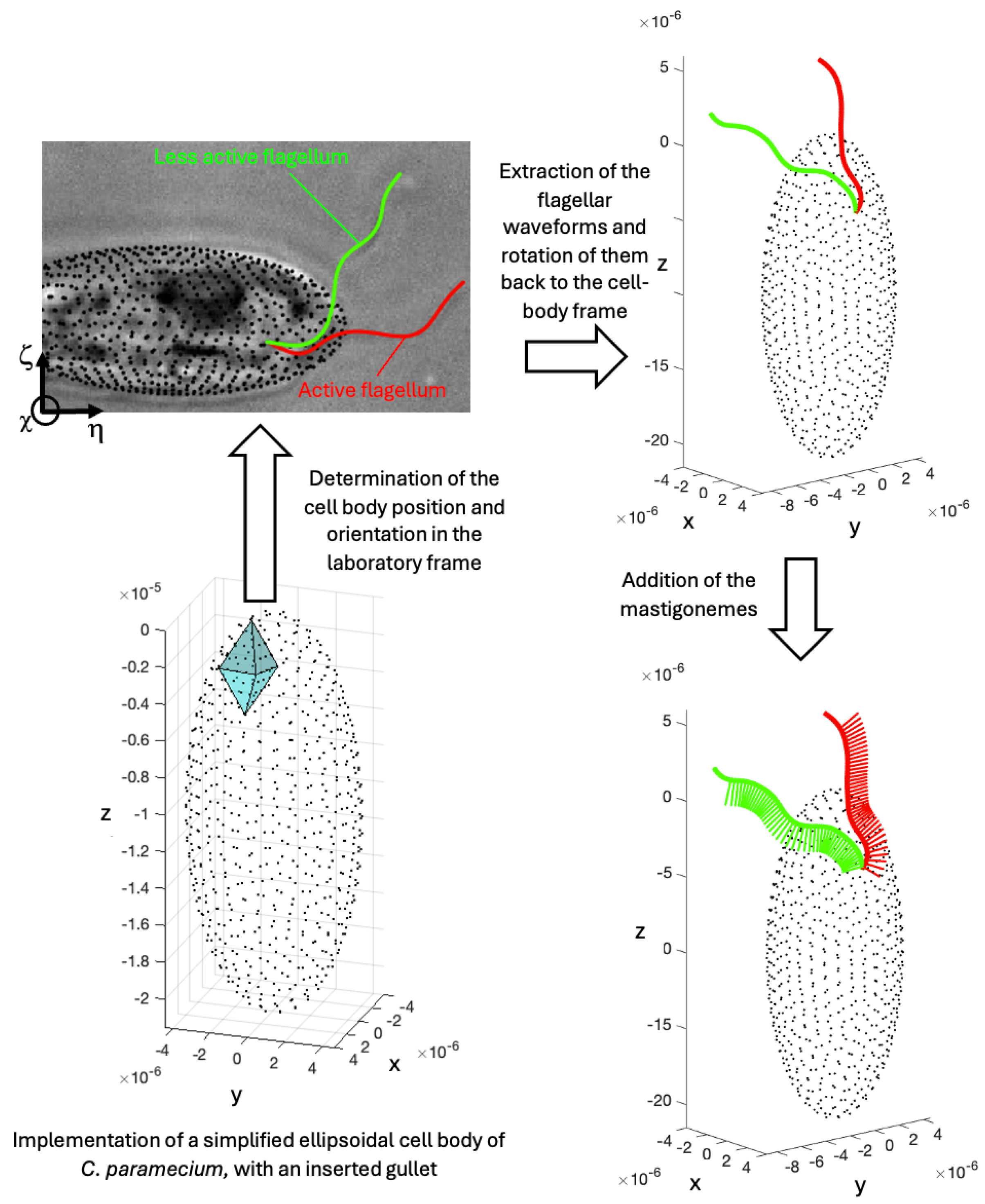
2.2. Acquisition of the Flagellar Waveforms from Phase-Contrast Microscopy and High-Speed Imaging

We used high-speed video phase contrast microscopy via a Princeton Instruments Kuro2048 camera (Teledyne Princeton Instruments, Trenton, NJ, USA), recording between 400 to 800 frames per second, to extract the cell’s swimming stroke, i.e., its flagellar waveforms over time. Magnifications of 20× and 40× were used to categorize overall cell motion during two main swimming behaviors, forward swimming and reorientation. Further studies using 100× magnification (with a depth of field of 410 nm) were also able to visualize the two flagella of C. paramecium during these swimming behaviors.
We first tracked the centerlines of the flagella when they were in the focal plane using ImageJ software (version 2.14.0/1.54f), coupled with the Kappa plugin, for curvature analysis. The curves are interpolated from control points placed manually on the in-focus flagella [42]. Once the control points are defined on each frame, a corresponding B-spline curve is generated to fit the points. The B-spline curves then comprise a frame-by-frame representation of the flagella waveform.

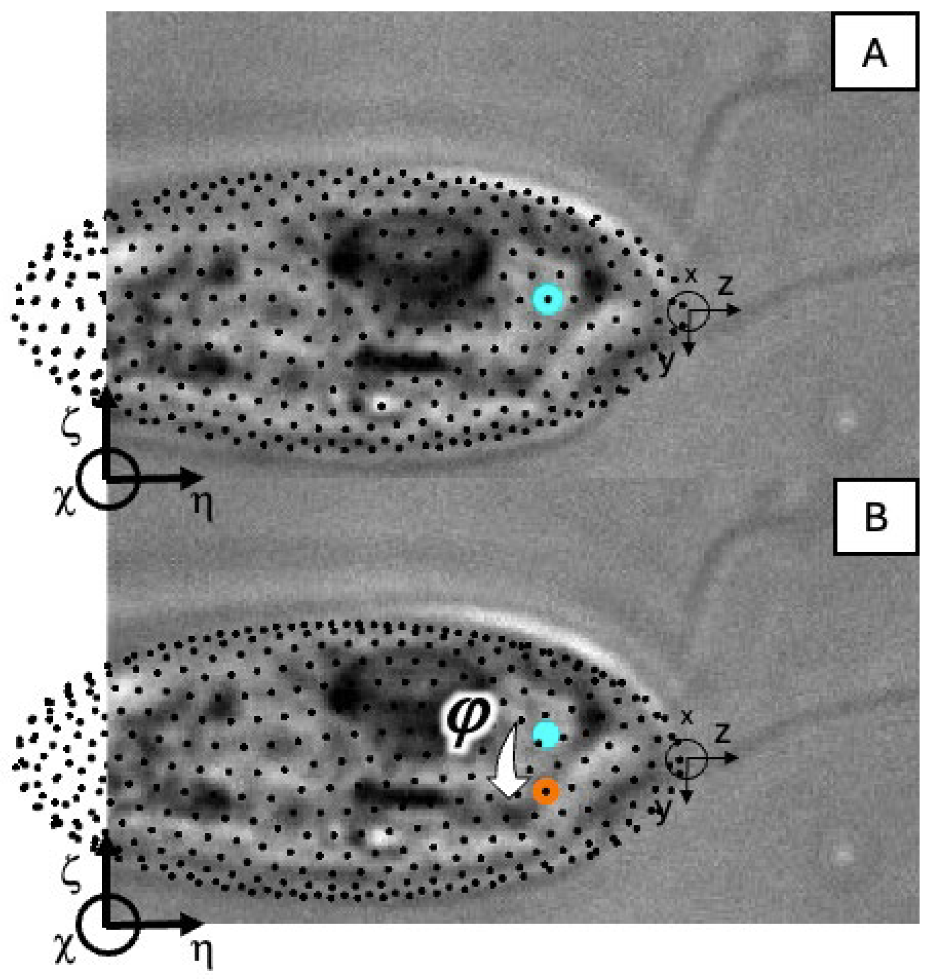
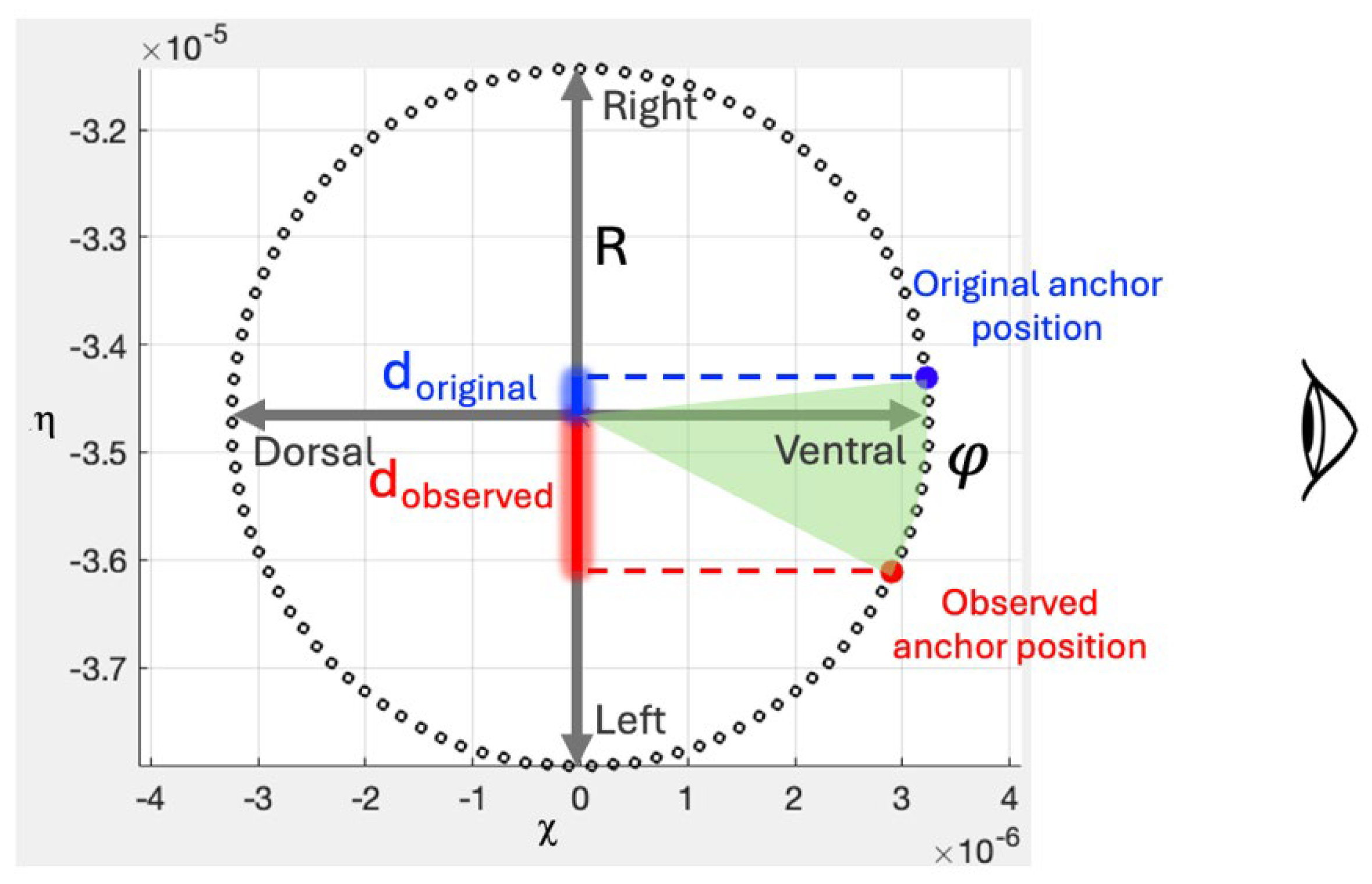
2.3. Tracking the Cell Body Position and Orientation

We used ImageJ (version 2.14.0/1.54f) to manually select the apical point of the cell body at each frame. The position of the apical point defines the translational position of the cell in the two-dimensional imaging plane.
We used a custom Matlab (version R2023b) GUI to draw an ellipse over the shape of the observed cell body in each frame. Cell body reorientation is described by a turning angle around the x-axis, as shown in Figure 1. The turning angle is the difference in the ellipse orientation between the initial frame and the frame of interest. The specification of the full three-dimensional cell body orientation requires another angle (φ) corresponding to the rotation of the cell around its longitudinal axis (the z-axis in Figure 1). To track the longitudinal angle φ, we used Image J software to track the position of the attachment point of the two flagella to the cell body. This involved manually placing the attachment point position on each frame of the video of interest. Through meticulous frame-by-frame analysis, we ensured accurate localization of the attachment points throughout the entire video sequence (Supplementary Video S2). As the cell rotates around its longitudinal axis, the location of the attachment point in the ellipse changes. We used a MATLAB error-minimizing solver that iteratively determined the longitudinal rotation angle necessary to minimize the distance between the observed anchor point in the frame of interest and the original anchor point marked in the first frame, rotated by the turning angle and then rotated by the longitudinal angle φ around the cell body z-axis (see Figure A1).
Due to the transparency of biological materials observed through phase-contrast microscopy, the longitudinal rotation may be perceived as either counterclockwise or clockwise around the z-axis, depending on whether the ventral side, with the flagellum anchor, is towards or away from the observer, respectively (see Figure A2). Therefore, for each frame, we obtained two rotation angles, φ and φ’, to align the anchored flagella with their observed shapes. φ represents the counterclockwise rotation needed if the cell initially presented its ventral side to the observer, while φ’ represents the clockwise rotation required if the cell presented its dorsal side to the observer. Additionally, we smoothed the values of φ and φ’ using a four-frame moving average to minimize abrupt rotations that could affect subsequent kinematic analyses.
We additionally quantified the uncertainties linked to our experimental observations by repeating the manual acquisition of the cell’s turning angle and position over time. For the net displacement, we chose five frames from our main video of interest and manually determined the position of the apical point five times for each frame. The standard deviation of the net displacement of the apical point from its original location provides an estimate of the uncertainty of the net displacement for each frame. Averaging these provides a typical uncertainty of the net displacement of ±124 nm, which is approximately the size of one pixel. For the turning angle, we drew ellipses around the cell body five times for each of these five frames using the Matlab GUI. The standard deviation of the turning angle obtained from these five measurements provides an estimate of the uncertainty of the turning angle in each frame. Averaging these yields a typical uncertainty in the turning angle of ±0.6°.
We used the error propagation formula to assess the uncertainties associated with finding the rotation angles φ and φ’, which can be derived from projecting the distance between the original and observed anchors and the frontal axis on the ventro-dorsal axis, when looking at a cross section of the cell body (see Appendix B for details), yielding a typical uncertainty of ±1.4 degrees for the longitudinal rotation angles.

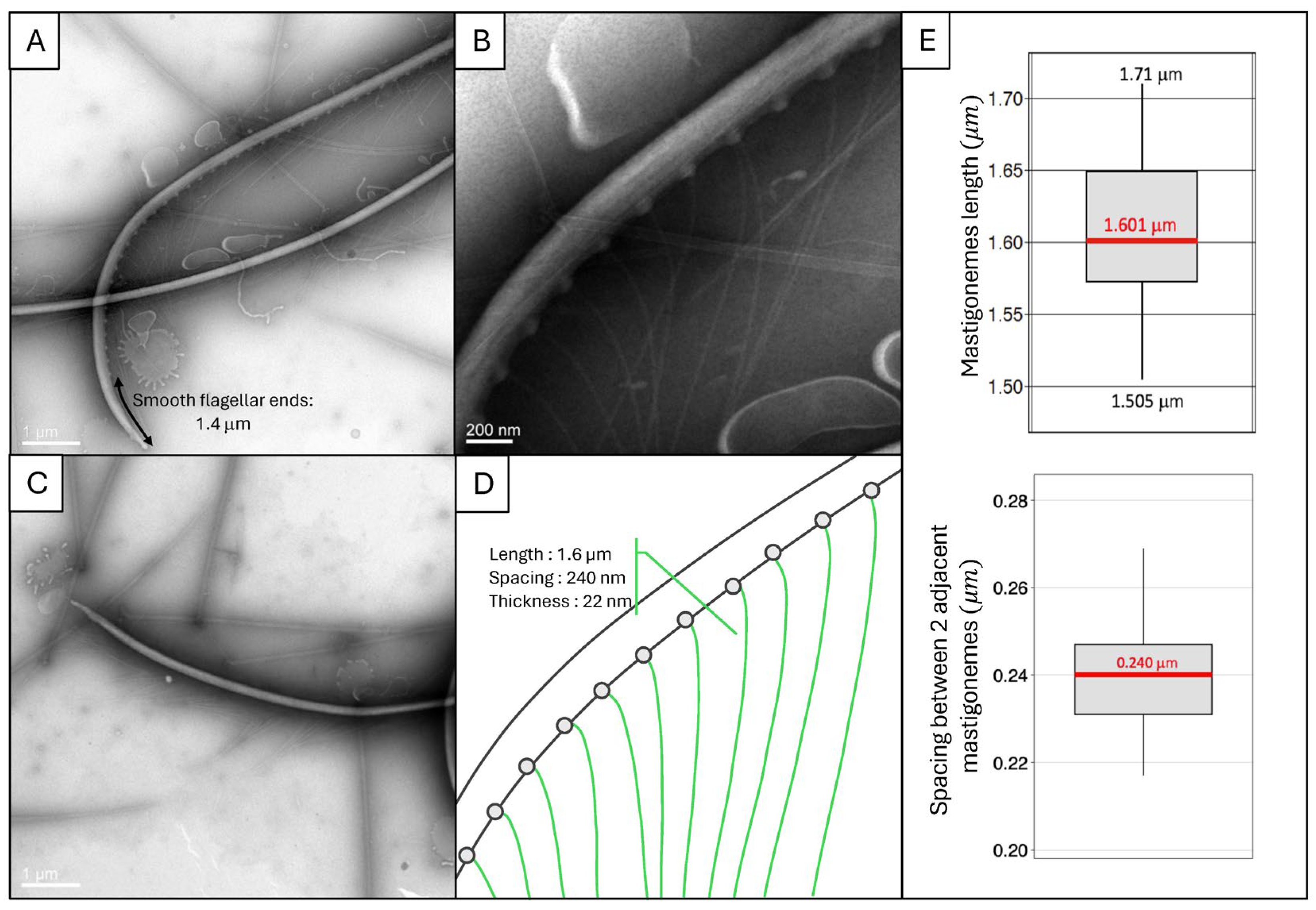
2.4. Acquisition of the Cell Body and Flagellar Ultrastructures Geometry from Observations Using Electron Microscopy

Phase contrast microscopy allows for the observation of flagellar waveforms but fails to reveal the flagellar hairs and their orientation due to the absence of labeling. Therefore, we employed electron microscopy to measure the cell body, flagella, and mastigonemes of Chilomonas paramecium.
Scanning electron microscopy (SEM): We used SEM to study the general morphology of the cells. The samples were critical-point dried and coated with 10 nm of Au/Pd. We used a Zeiss GeminiSEM-300 (Oberkochen, Germany) device, operating at 10 kV, with an InLens BSD detector at 33 nm pixel size to capture the SEM images. This technique provided detailed dimensions of the cell body and flagella but did not preserve the thin external hairs on the flagella.
Transmission electron microscopy (TEM): Despite recent attention to the resolution revolution resulting from significant advances in cryo-electron microscopy [43] (cryo-EM), negative staining electron microscopy remains a powerful technique, as it allows for the relatively simple and quick observation of microorganisms, macromolecules, and macromolecular complexes through the use of a contrast-enhancing stain reagent. We employed TEM with negative staining to observe the fine structures of the mastigonemes. The cultured specimens were pelleted by gentle centrifugation (5 min, 600× g), the supernatant was removed, and 3.5 µL of the concentrated sample was placed on carbon-coated grids. The cells were stained with a 1% uranyl acetate solution before observation. We used a JEOL-JEM 1400 plus electron microscope (Tokyo, Japan), operating at 120 kv, and a Gatan ultrascan camera (Pleasanton, CA, USA), with a 2.4 nm pixel size, to capture the TEM images. This protocol allowed us to measure the dimensions and distribution of the mastigonemes, although it often resulted in cell body deformation due to ejectosome discharge, complicating the detailed examination.
Measurement and analysis: We used ImageJ software to manually measure the flagella’s thickness and the half-diamond-shaped gullet’s dimensions. Similarly, the length of the mastigonemes was measured using the TEM images.

2.5. Prediction of Swimming from Flagellar Motions Using the Method of Regularized Stokeslets

We perform numerical simulations that take the motion of the flagella with respect to the cell body frame (in which the cell body is stationary) as input and assume zero total force and zero torque conditions (a neutrally buoyant cell body with uniform density). The simulations output the velocity and rotation of the swimmer, which are then used to construct the trajectory of the cell body over the time of interest.
The method using regularized Stokeslets [44,45] has been employed extensively to study swimming microorganisms [46,47,48,49,50,51]. In this approach, the flow is described as a result of localized forces at the surface of the cell body and flagella. The surface of the cell body and flagella is discretized by regularized Stokeslets, which are fundamental solutions to the Stokes equation for applied localized force distributions ϕε, smooth approximations for point forces fα:
ϕ ε r = 15 ε 4 f α 8 π | r | 2 + ε 2 7 2
The parameter ε represents the width of an individual regularized Stokeslet’s force distribution. The total flow velocity at position r due to N regularized Stokeslets is:
v i r = j = 1 3 α = 1 N S i j r r β f j β
where {i, j} = {1, 2, 3} run over coordinates {x, y, z}. rα is the position of the Stokeslets with localized force fα, and the regularized Stokeslet is:
S i j r = ( | r | 2 + 2 ε 2 ) δ i j + r i r j 8 π μ | r | 2 + ε 2 3 2
To apply Equation (2), we need to find the strength of the localized forces of the Stokeslets on the surface of the cell and the flagella. To do so, we first express the velocity at each point of the surface in terms of the swimming velocity and rotation of the swimmer. We use the apical point of anterior region of the cell body as the origin of the fixed body frame. The velocity at each of the N positions rα can be written:
v r α = V + Ω × r α + L α ˙
where V and Ω are the swimming and angular velocities, respectively, rα represents the Stokeslet positions placed on material points of the surface in the fixed body frame, and L α ˙ shows the velocities of the Stokeslets, with respect to the fixed body frame specifying the swimming stroke. In our case, the flagella are beating relative to the cell body, so L α ˙ is zero for α   corresponding to positions on the cell body but nonzero for α corresponding to positions on the undulating flagella.
Evaluating Equation (2) at r = rα for each of the rα leads to 3N equations with 6 N unknowns (3 N components of v(rα) and 3 N components of fα. Equation (4) adds six more unknowns (V and Ω) and 3 N more equations. To solve the system, we need six additional equations coming from the zero total force and zero total torque conditions for a free swimmer in the fluid, ∑αfα = 0 (three equations) and ∑αrα × fα = 0 (three equations). This reduces the problem to a linear system of equations in the fixed body frame that can be solved at each timestep. In particular, we obtain the cell body translational and rotational velocities (V and Ω) at each timestep. Details of our implementation can be found in the work of Martindale et al. [52].
To apply the method using regularized Stokeslets to C. paramecium, we discretized the surface of C. paramecium. The cell body is represented as an ellipsoid with the addition of a “gullet” (also sometimes called a “furrow”), a diamond-shaped cavity located towards the apical end on the ventral side of the cell, from which the two flagella emerge (Figure 2). The dimensions of the cell body and gullet follow those obtained from electron microscopy.
To generate the flagellar geometry in the body-fixed frame, at each timestep, we use the B-spline representing the flagellar centerline and rotate it back to the orientation of the cell body in the first timestep corresponding to the initial video frame, where the body-fixed axes {x, y, z} are defined in Figure 2. In other words, we rotate the B-spline around the z-axis by −φ or −φ’ (for the two cases of ventral orientation, respectively) and then around the x-axis (which is perpendicular to the image plane) by the negative of the turning angle.
Since the flagella cannot overlap in space, we shift the flagellar bases by 1/10th their diameter (220 μm) in the ±y directions. Doing so avoids numerical issues that arise when Stokeslets are placed very closely together. We then place N i n i t i a l positions at fixed distances ( d f ) along this body-frame centerline, and extrude the tubular surface of the flagella by forming a circle centered at each of the N i n i t i a l positions, in 3D and perpendicular to the centerline, with a diameter of D t (200 nm, from the EM observations in Results, Section 1). Finally, each circle is discretized into eight equally spaced points.
Mastigonemes were added perpendicularly to the surface of the tubes, either in the beating plane or in the plane perpendicular to the beating plane (depending on the mastigoneme geometry being tested) and were discretized into N s t , m points along their centerlines ( N s t , m = m a s t i g o n e m e s   l e n g t h m a s t i g o n e m e s   r a d i u s ) equally spaced by the distance d m , equal to the average radius of C. paramecium mastigonemes (from the EM observations in Section 3.1). The numerical values for the parameters used in the simulation are listed in Table 1.
A regularized Stokeslet is placed at each discretization point. The velocities of the Stokeslets on the flagella and mastigonemes ( L α ˙ , in Equation (4)) relative to the cell body are calculated by taking the displacement of that Stokeslet position from the previous timestep and dividing it by the timestep.

3. Results

3.1. Experimental Observations

3.1.1. Experimental Observations of C. paramecium Geometry

From our electron microscopy studies, we observe that the cell body of C. paramecium is 8 μm in thickness, 9 μm in width, and 21.5 μm in length. We describe it as a prolate ellipsoid of minor axis 8.5 μm and major axis 21.5 μm. The flagella length is between 15 to 20 μm, with a thickness of 200 nm (Figure 3 and Figure 4). There are mastigonemes on both flagella, and on each flagellum, mastigonemes are distributed equidistantly and unilaterally. They exhibit a spacing of 240 nm and their length is 1.6 μm in average (with minimum and maximum values of 1.505 to 1.71 μm, respectively), in concordance with the previously reported mastigoneme lengths in cryptophytes between 1.5 and 2 μm [30,31,32]. We additionally noticed that the mastigonemes arrays stop 1.4 μm from the tip of the flagella, leaving smooth end portions. However, our observations close to the cell body were hindered by the charging of bulk material discharged by the cell body, obstructing our view of the mastigoneme array near the gullet. Therefore, the distance at which the mastigonemes begin to emerge from the flagellum near the cell body remains uncertain.
Both flagella emerge from a half-diamond shaped opening, called the “gullet”, which is situated ventrally, on the antero-left side of the cell body, and tends to impart an asymmetrical shape to the cells [33] (Figure 3). The gullet depth is 1.72 μm, the length is 4.98 μm, and the width is 2.25 μm. The simplified cell model derived from these observations is presented in Figure 5.
We use these geometrical parameters as inputs to build our simulations, based on the structural characteristics of the cell body, flagella, and mastigonemes, together with the extracted flagellar waveforms (for propulsion) and cell body motion from the video of interest.

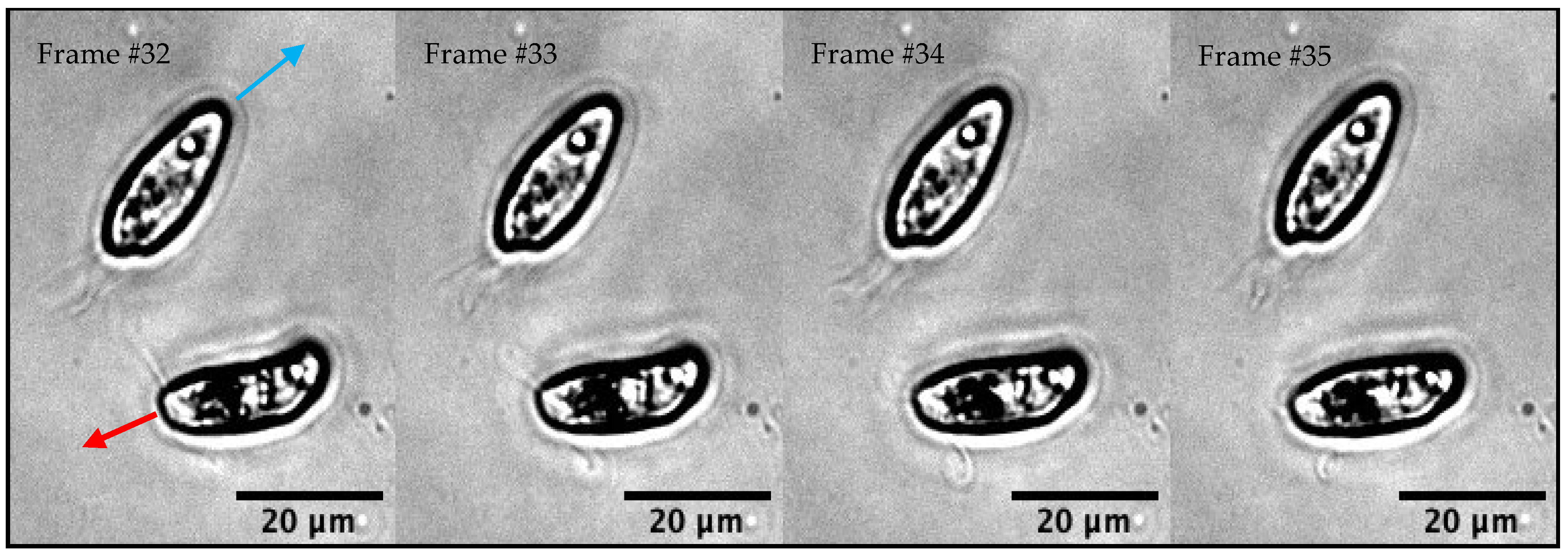
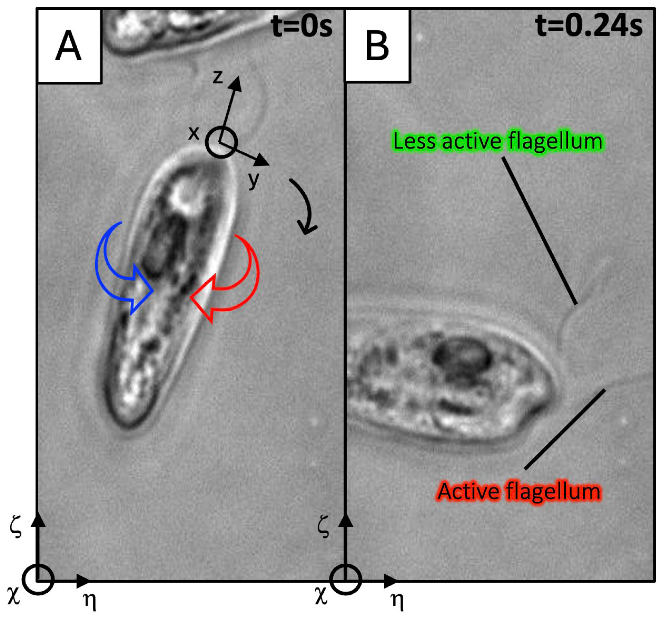
3.1.2. Experimental Observations of C. paramecium Motility and Flagellar Waveforms

C. paramecium displays two distinct swimming behaviors: forward motion and reorientation events. During forward swimming (toward the anterior end of the cell body, Supplementary Video S5), the flagella project from the ventral side of the cell body, exhibiting alternating brightness and darkness as parts of them move in and out of the focal plane, which indicates that they undergo breaststroke-like motion, with helical traveling waves. This flagellar motion is coupled with the cell body moving from side to side, while also rotating around its longitudinal body axis (Supplementary Video S6). Our observations are in good agreement with the swimming behavior described by Christensen [53] as “recoiling”.
When encountering an obstacle, we observe, in accordance with previously reported observations [54], that the organism reverses the direction of motion by projecting both flagella toward the anterior end of the cell body (Figure 6, Supplementary Videos S1 and S2), moving backward for a small distance (toward the posterior end of the cell body). Subsequently, the cell turns, which changes the swimming direction. This sequence is repeated until a clear field is achieved. In Supplementary Videos S1 and S2, during the backward motion, we observe wave-like deformations, which are of consistent sharpness and color, propagating along the flagella, indicating that they remain close to the focal plane. Since the flagella diameter is 200 nm and the depth of field is 410 nm, this suggests that both flagella of C. paramecium are beating in a 2D plane during the backward motion of the reorientation events, in contrast with the helical waves of the forward motion.
According to Votta [54], longitudinal rotation occurs in the faster moving organisms, and could be due to at least three mechanisms: (1) unequal flagellar lengths [55], (2) one flagellum remaining motionless, and the organism locomoting with the other flagellum alone, (3) asymmetry of the body of the organism. In contrast, in some instances, we also observed cell body rotation around the longitudinal axis when the cells are moving slowly during a reorientation. Our observations differ slightly from those expected for the proposed second mechanism, i.e., although the flagella are not whipping with equal amplitudes in our studied video, neither remains motionless. Instead, we can differentiate an “active” flagellum with higher amplitudes from a “less-active” flagellum with smaller amplitudes, but the cells do not remain motionless, as previously suggested.

3.2. Flagellar Waveform Extraction, Kinematic Analysis, and Simulation Inputs

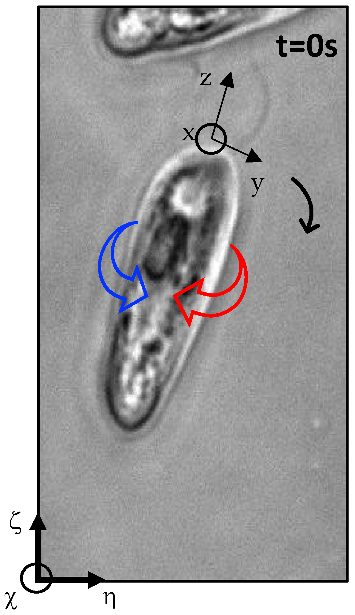
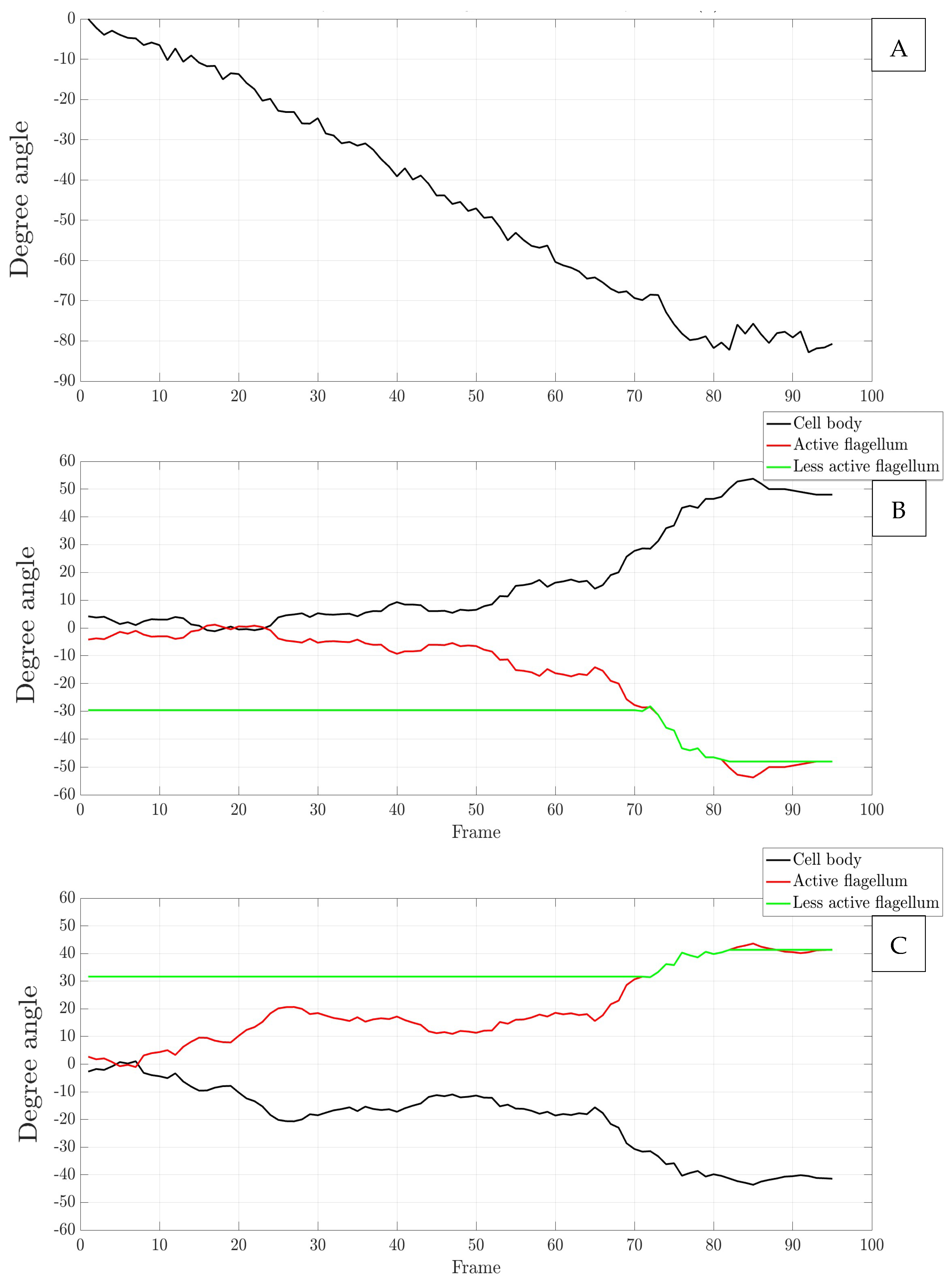
3.2.1. Description of the Video of Interest

Among the various swimming strokes observed in C. paramecium, we focused our attention on a particular reorientation event in which both flagella are distinctly visible. This event occurs when the cell predominantly presents one side to the observer, although it remains uncertain whether this side is ventral or dorsal, due to the transparency of the cells (see Supplementary Video S1). In the extended version of the video (Supplementary Video S7), the cell initially propels itself forward towards a neighboring cell, a motion lasting 0.22 s. Subsequently, it quickly interacts with the obstacle for a brief duration of 0.043 s before initiating a simultaneous backward movement and the beginning of the reorientation event. During the first half of this event, the cell turns clockwise around its dorsoventral axis (x-axis). Subsequently, an additional longitudinal rotation around the longitudinal axis (z-axis) is observed until the completion of the reorientation process. Upon the completion of this sequence, the cell has turned and rotated over a total duration of 0.24 s, achieving a clear field of view (Figure 7).
The video of interest (Supplementary Video S1) was selected for its outstanding display of both flagella and cell body movement, and it includes 95 frames of Supplementary Video S7, during which the cell is reorienting. In the first frame of the video of interest (Figure 7, left panel), the cell’s orientation could either present its ventral or dorsal side to the observer. By the end of the video, the cell shows its lateral side to the observer, it has reoriented clockwise around the laboratory χ-axis (perpendicular to the imaging plane, see Figure 7 by a turning angle of 80.7° from its original orientation, and its apical point has translated 19 μm along the positive η-axis and the negative ζ-axis of the laboratory ηζ plane (the imaging plane). Simultaneously, the cell body rotates longitudinally around the body-fixed z-axis. The evolution of the longitudinal rotation angles φ and φ’, together with the turning angle of the observed cell, are reported in Figure 8.

3.2.2. Analysis of Flagellar Waveform Variation

To compute the movement of C. paramecium at each timestep, we need to specify the waveform of both flagella. We observed that the flagella have different amplitudes during our video. The highlighted “active flagellum” in Figure 7 has a higher amplitude than the highlighted “less-active flagellum” during the first two-thirds of the video. Moreover, the less-active flagellum is fully in focus for only a small portion of the video (during 176 ms, from frame #71 to frame #82), unlike the active flagellum that beats within the depth of focus, in 2D, during the whole video. For input into the simulations, due to the limited availability of in-focus flagellar waveforms for the less-active flagellum, we opted to extrapolate the out-of-focus shapes from the in-focus samples by looping over the 11 observable waveforms for the entire video. Since the less-active flagellum is not in focus outside of frames #71–#82, it cannot have rotated by the same longitudinal angle as the cell body. In the absence of definitive data on the longitudinal rotation of the less-active flagellum, we assume that before and after frames #71–#82, it maintains a constant angle relative to the cell body, i.e., its longitudinal rotation is shown by the green curves in Figure 8B,C for ventral and dorsal presentation, respectively.
To create inputs for the simulations, we additionally constrained the lengths of the extracted flagellar shapes in order to best represent the flagellar morphology of C. paramecium. Although flagella are inextensible and should have constant length, the image analysis and extraction process described in the methods resulted in variations in flagellar lengths. We observed a length range of 13.46–15.55 µm for the less-active flagellum and 10.82–15.15 µm for the active flagellum. To resolve this discrepancy, we only retained the proximal portion of the extracted flagellum with a constant length for each flagellum. For the less-active flagellum, we chose to take the smallest length observed: 13.46 µm. For the active flagellum, we noticed one outlier waveform of the flagellar length range at timestep #69. However, thanks to the periodic nature of the propagated waves, we were able to interpolate a flagellar shape for this timestep from its earlier and later positions. Having then removed the short outlier waveform, the smallest value of the remaining lengths of the active flagellum was 12.09 µm, which we chose as the length of the active flagellum in our simulations.

3.3. Numerical Study of the Hydrodynamic Effects of Rigid Mastigonemes in C. paramecium

With the detailed kinematics of the observable flagella, we can simulate the swimming behavior of the observed reorienting cell using the regularized Stokeslets method. This simulation predicts the velocities and orientation of the swimmer for both possible initial orientations. The model takes as inputs the structural characteristics of C. paramecium and the waveforms of its flagella relative to the cell body, as recorded from the video of interest. The resulting outputs are the trajectories that the simplified cell would swim considering the presence of different configuration of mastigonemes on its flagella.

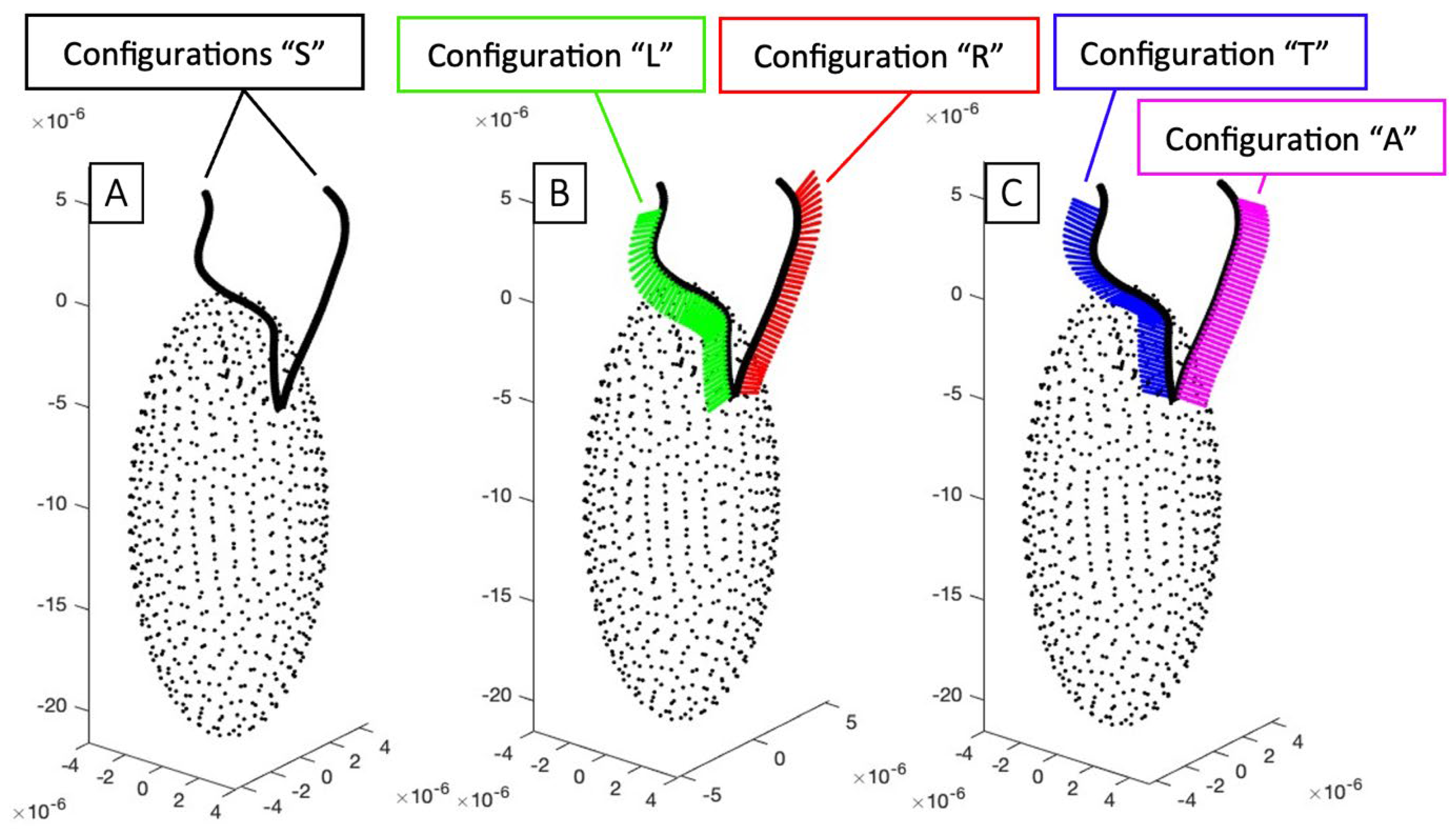
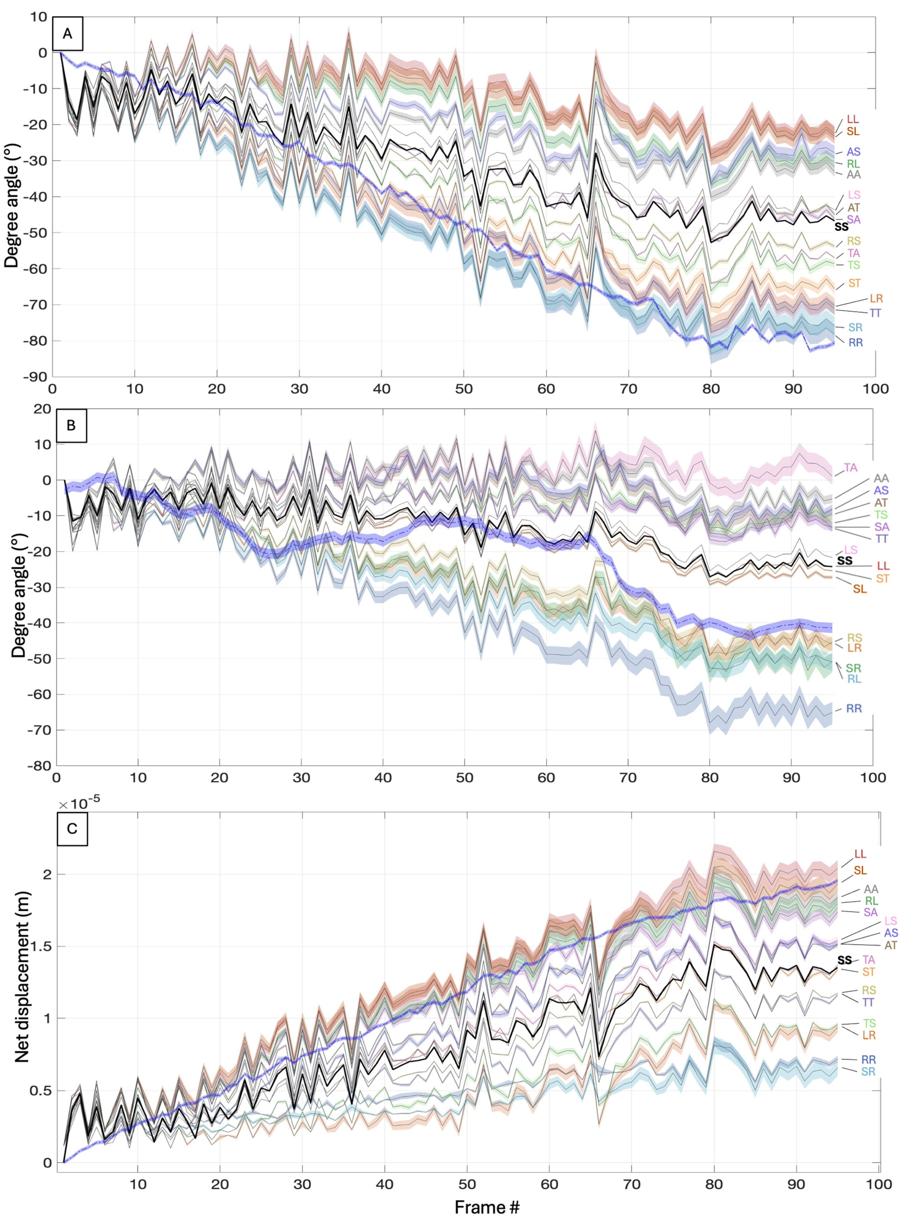
3.3.1. Mastigoneme Configurations

To investigate the hydrodynamic effect of mastigonemes in C. paramecium, we tested five configurations on each flagellum. Since the TEM images confirmed that C. paramecium displays one row of mastigonemes on each flagellum (shown in Figure 9), these configurations involved varying the orientation of the hairs on each flagellum, including:
  • Mastigonemes oriented toward the right in the beating plane, labeled as “R”.
  • Mastigonemes oriented toward the left in the beating plane, labeled as “L”.
  • Mastigonemes oriented toward the cell body in the plane perpendicular to the beating plane, labeled as “T”.
  • Mastigonemes oriented away from the cell body in the plane perpendicular to the beating plane, labeled as “A”.

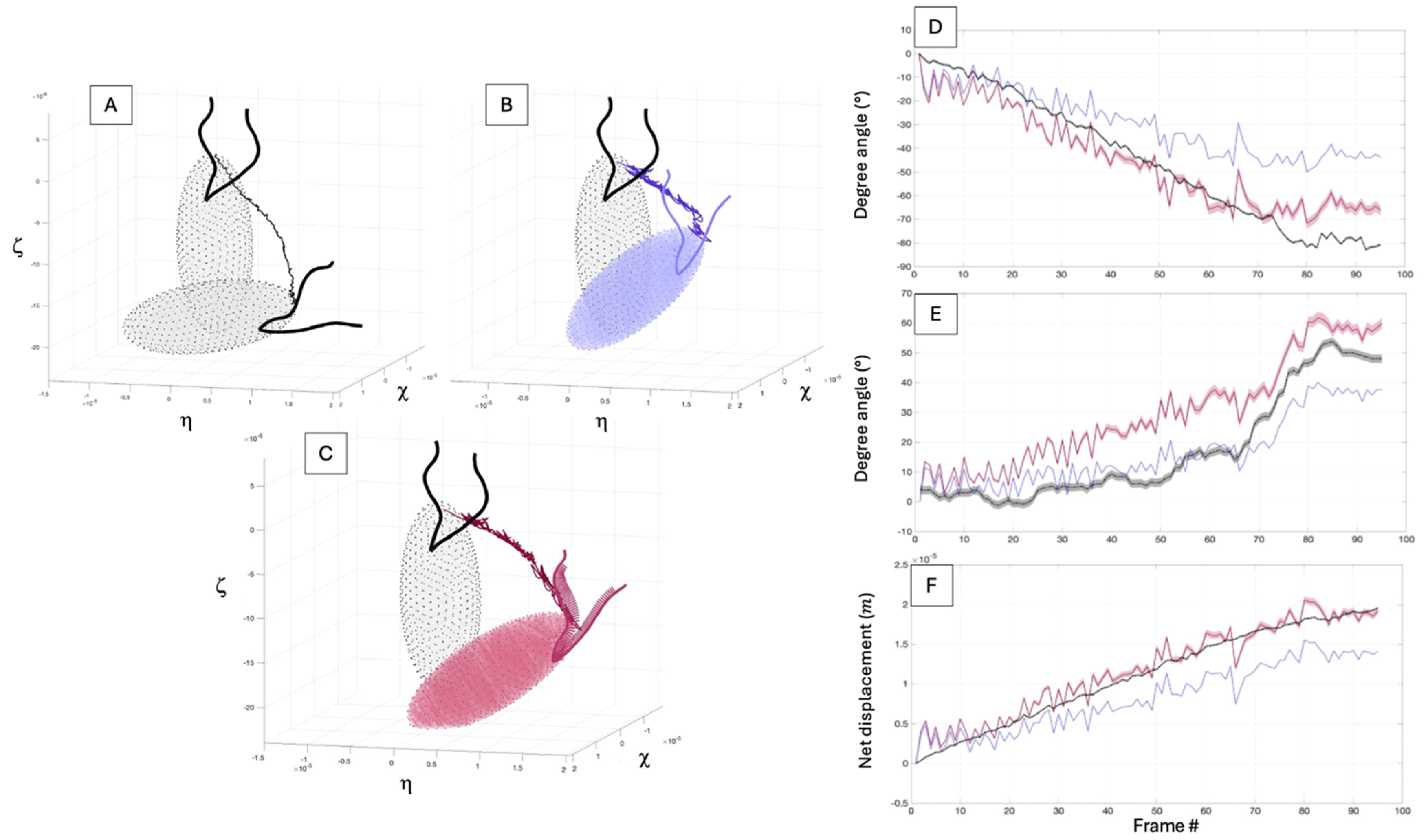
3.3.2. Simulation Overview

We generated 17 distinct configurations of flagellar hairs in our simulated model of C. paramecium for both gullet orientation cases. Anticipating that rigid mastigonemes and their orientations would influence the cell’s direction, we aimed to identify arrangements producing comparable displacement and turning angles to those observed in our selected video.
The translational and rotational velocities (V and Ω ) are the outputs from the use of the regularized Stokeslets method. From those, we can simulate the movement of the cells and predict the trajectories and orientation of the cells over time. Particularly, we compared the net displacements and the orientation angles between those of the video of interest and our simulations.
The evolution of the net displacements is determined by tracking the apical point of the cell body in both our simulations and the ellipsoid overlayed on the observed cell body from the video of interest. The comparison of orientations involves comparing the evolution of rotation angles around the x-axis (the turning angles) and around the z-axis (the longitudinal rotation angles) between the simulated and observed cell.
As discussed in Section 3.1, measurements obtained from EM observations revealed the mastigonemes to be 1.6 μm long, on average, with smooth flagellar tips measuring 1.4 μm. However, the starting position of the mastigoneme arrays is unknown due to the charging and deformity of the cell body under transmission electron microscopy. To simulate mastigoneme-bearing cell motion, we used the average mastigoneme length and initiated hair arrays at the flagellar bases in the “standard” configuration.
In addition to the standard configuration, we further tested the results’ robustness by varying the structural parameters. We tested mastigoneme lengths of 1.505 μm and 1.71 μm, in addition to the standard length of 1.6 μm. These lengths correspond to the minimum and maximum observed mastigoneme lengths in our TEM images (Figure 7). We also tested configurations in which the mastigoneme arrays started 1.4 μm from the flagellar base (the same length as the smooth flagellar tips) instead of at the flagellar base. Altogether, we tested four configurations—the standard configuration, the configuration with shorter and longer mastigoneme lengths, and the configuration with 1.6 μm long mastigonemes that start 1.4 μm from the flagellar base. The results below report positions of the standard configuration, with shaded uncertainties corresponding to the maximum and minimum of these four configurations to indicate a likely range of numerical results, given uncertainties regarding the mastigoneme length and configuration.

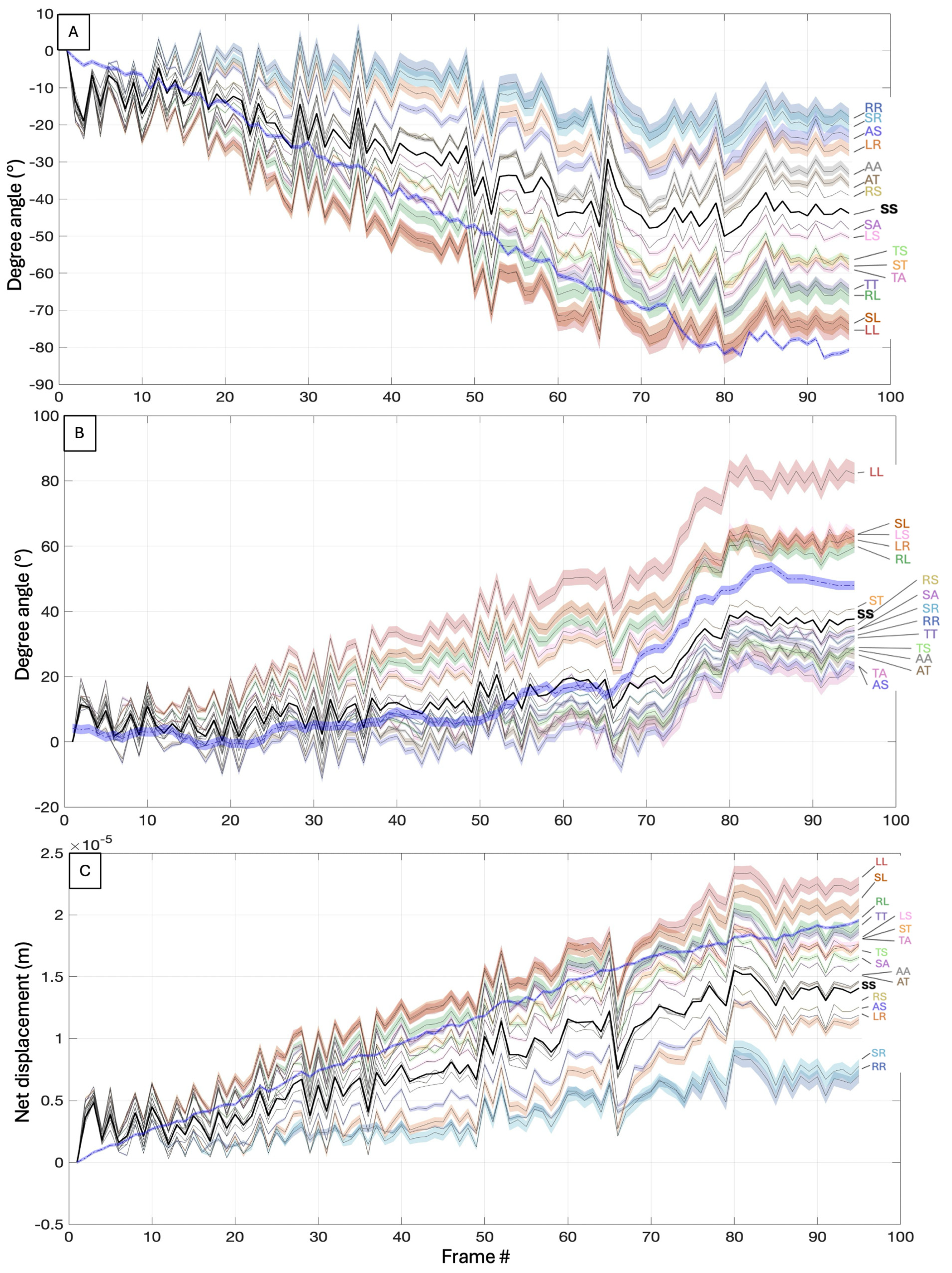
3.3.3. Numerical Results

This section presents the results of each of the 34 study cases, each featuring different mastigoneme configurations and the initial ventro-dorsal orientation of the cell body. Our focus will be on comparing the temporal evolution of their turning and rotation angles around the y and z axes, along with tracking the progression of their net displacement over time.
We will first start by illustrating the output motion dynamics of two standard cases: mastigoneme configurations “SS” and “RL” of a ventrally presented cell, showcased in Figure 10.
The simulation output consists of frame-by-frame positions and orientations of the simulated cell, from which trajectories and orientations can be determined. Upon analysis of these cases, we observed that both the “SS” and “RL” configurations rotate clockwise relative to their x-axis, similar to experimental observations. However, differences in turning angles and net displacement are evident between the two configurations. In Figure 10, panel D–F, we plot the turning angle, longitudinal angle, and net displacement as a function of time for the “SS” and “RL” configurations. The solid black lines indicate the experimental measurements for these parameters, with grey shaded areas corresponding to the estimated experimental uncertainty expressed in Section 2.3. For the numerical results, the shaded regions show the uncertainties estimated from the robustness studies described above. Configuration “RL”, featuring mastigonemes arranged in a single row on each flagellum within the flagellar beating plane, better reflects the behavior of the recorded cell, while configuration “SS”, with smooth flagella, deviates from the observed motion. These discrepancies highlight the impact of mastigoneme arrangement on the cell’s dynamics and suggest the need of ranking mastigoneme configurations based on their closeness to the observed cell behavior.
To assess the trajectories of all the mastigoneme configurations, in Figure 11 and Figure 12, we plot the turning angle, longitudinal rotation angle, and net displacement of the apical point as a function of time for all tested mastigoneme configurations. Figure 11 shows the results, assuming a ventral presentation of the cell towards the observer, while Figure 12 shows the results, assuming a dorsal presentation of the cell towards the observer.

4. Discussion

Examining Figure 11 and Figure 12, it is apparent that all the curves exhibit similar qualitative features, such as the sign and general increase of the turning angle and the nearly linear growth in net displacement, and that these features match those observed in the experimental video. However, the quantitative rotation angles and net displacements differ for smooth flagella without mastigonemes and for the various configurations of the mastigonemes. From this, we conclude that the overall motion of the flagella dominates the qualitative features of reorientation—there is no gross change, such as reversal, as thrust produced by mastigonemes. At the same time, however, the presence of mastigonemes has a clear hydrodynamic effect, causing some configurations to reproduce experimental results more closely than others, and in particular, yielding better results than those for smooth flagella without mastigonemes.
Next, we determine which mastigoneme configurations more closely match the experimental results. When a ventral presentation is assumed (Figure 11), the observed turning angle (Figure 11A) is best matched by the SL, LL, TT, and RL configurations. Note that while the TT and RL configuration do not match the observed turning angle at the end of the time frame, they provide better results than the SL and LL configurations throughout the middle of the time frame. Similarly, the observed longitudinal rotation angle (Figure 11B) is best matched by the SL, LS, LR, and RL configurations, while the observed net displacement (Figure 11C) is best matched by the LL, SL, RL, and TT configurations. Notably, the SL and RL configurations are among the best matching scenarios for all three metrics, and performing significantly better than the SS case without mastigonemes. Since the EM imaging shows that both flagella have mastigonemes, this suggests that the RL configuration is the most likely. Thus, these results reinforce the belief that mastigonemes have a hydrodynamic effect.
When a dorsal presentation is assumed (Figure 12), the observed turning angle (Figure 12A) is best matched by the RR, SR, TT, LR, and ST configurations, and the observed net displacement (Figure 12C) is best matched by the LL, SL, AA, RL, and SA configurations. Interestingly, the best performing configurations for the observed turning angle tend to be the worst performing for the net displacement, and vice versa, i.e., the results of these two metrics are contradictory. Compared with the performance of the mastigoneme configurations in the ventral presentation, this result suggests that the cell body had a ventral presentation in the experiment. This conclusion is reinforced by the unclear results when ranking the performance of the longitudinal rotation angle for the dorsal presentation (Figure 12B). For that metric, one set of configurations (LS, SS, LL, ST) performed well only in the middle of the time frame (frames 40–65), while a different set (RS, LR, SR, RL) performed better in the earlier and later frames.

5. Conclusions

Our results suggest that mastigonemes in the cryptophyte C. paramecium do indeed have a hydrodynamic effect. This is result similar to that for other protists, such as Ochromonas [35,37,56], but may be in contrast to that for Chlamydomonas reinhardtii; some studies have shown that the hair-like projections on Chlamydomonas flagella do not contribute to thrust enhancement [38], but other recent studies have shown that mutants of Chlamydomonas, lacking mastigonemes, exhibit a statistically significant reduction in swimming velocity [29,57,58]. Note that the chlorophyte C. reinhardtii differs from C. paramecium in that it features mastigonemes that are more flexible, and C. reinhardtii has a more spherical cell body compared to the more elongated shape of C. paramecium, which could also influence swimming dynamics [59]. Our findings in this manuscript further emphasize the potential hydrodynamic role of mastigonemes in flagellar motility, which aligns with the observations in our study. However, it seems that the hydrodynamic effects may not be generalizable across flagellated protists, as these range from none or minimal (Chlamydomonas [38]) to qualitative (Ochromonas [35,37,56]) and in between (Chilomonas); instead, they seem to be species-dependent, perhaps due to the differing morphology and properties of each species’ mastigonemes.
In general, future studies could address whether mastigoneme flexibility is important in determining their hydrodynamic effect. This could be accomplished both numerically, with simulations employing methods such as those developed by the authors of Ref. [60], as well as experimentally, such as by observing (under light microscopy) whether fluorescently stained mastigonemes deform during swimming. However, in C. paramecium, the hydrodynamic effect is more subtle than the thrust reversals predicted and observed for Ochromonas [35,37,56] and Phytophora cinnamomi [36]. These more subtle effects have also been examined, not only in the context of swimming, but also in regards to feeding [61,62] in protists. Our results add another example of the effects of mastigonemes on swimming behaviors, which could interact with other possible hydrodynamic and biological effects in a species-dependent fashion.

Supplementary Materials

The following supporting information can be downloaded at: https://www.mdpi.com/article/10.3390/hydrobiology3030012/s1, Video S1: Reorientation event. Video S2: Overlaid cell body without longitudinal rotation, initial anchor point and highlighted flagella. Video S3: Overlaid cell body with longitudinal rotation, initial anchor point and highlighted flagella. Video S4: Extracted flagellar motion in the cell-body frame. Video S5: 2 swimming behaviors or C. paramecium. Video S6: Cell body moving from side to side, while also rotating around its longitudinal body axis. Video S7: Reorientation event (long version).

Author Contributions

Conceptualization, H.C.F. and L.S.A.; methodology, L.S.A., L.N. and M.S.; software, L.S.A.; validation, H.C.F.; formal analysis, L.S.A.; investigation, L.S.A. and H.C.F.; resources, L.N. and M.S.; data curation, L.S.A., B.W., K.S., L.N. and M.S.; writing—original draft preparation, L.S.A.; writing—L.S.A. and H.C.F.; visualization, L.S.A.; supervision, H.C.F.; project administration, H.C.F.; funding acquisition, H.C.F. All authors have read and agreed to the published version of the manuscript.

Funding

This research was funded by US National Science Foundation grant number CBET-1805847. Computational resources were provided by the University of Utah Center for High Performance Computing.

Data Availability Statement

The raw data and code supporting the conclusions of this article will be made available by the authors on request.

Conflicts of Interest

The authors declare no conflict of interest.

Appendix A. Figures Depicting Longitudinal Rotation Angles

Figure A1. Determination of the longitudinal rotational angle around the z-axis from the movement of the anchor point. (A) Discretized cell body and anchor point (blue dot) from Frame #1, after rotating by the turning angle around laboratory-frame axis χ so that the body z-axis is in the same direction as in frame #75. (B) Discretized cell body and anchor point (orange dot) from Frame #75. The original anchor point from (A) (blue dot) overlaps with the observed anchor point (orange dot) after rotation around the z-axis by angle φ. In this example, it is assumed that the ventral side of the cell body is towards the observer.
Hydrobiology 03 00012 g0a1
Figure A2. Schematic of the two possible interpretations of the cell’s initial orientation. (A) If the cell is presenting dorsally to the observer, clockwise rotation by φ causes the attachment point to appear to move to the right. (B) If the cell is presenting ventrally to the observer, counterclockwise rotation by φ causes the attachment point to appear to move to the right.
Hydrobiology 03 00012 g0a2

Appendix B. Error Propagation for Uncertainties in Longitudinal Rotation Angles

The longitudinal rotation angles φ   and φ ’ are defined as a function of the observed projected distances between the anchor and the frontal axis of the cell body and the radius of the cross-section (Figure A3):
φ = f d o r i g i n a l , d o b s e r v e d = sin 1 d o r i g i n a l R + sin 1 d o b s e r v e d R
Both the position of the original anchor point, marked in the first frame, and the position of the observed anchor point in subsequent frames were obtained by manually marking the anchor on the image. To estimate the uncertainty of the anchor point position, we repeated the marking of the anchor point five times on the same five frames used to estimate the uncertainties of the net displacement and turning angle. The standard deviation of the position of these five measurements is taken to be Δ d o b s e r v e d for each frame. Δ d o r i g i n a l is obtained in a similar fashion for the first frame. By applying the error propagation formula to these standard deviations (A2), we calculated the uncertainty associated with determining the angles φ and φ’ for each of the five frames.
Δ θ = f d o r i g i n a l Δ d o r i g i n a l 2 + f d o b s e r v e d Δ d o b s e r v e d 2
Averaging these yields a typical uncertainty of ± 1.4° for the longitudinal rotation angles around the z axis.
Figure A3. Cross section of the cell body (initially presenting ventrally) showing the cell’s anatomical axis and the projected distance between the center and the observed and original anchor.
Hydrobiology 03 00012 g0a3

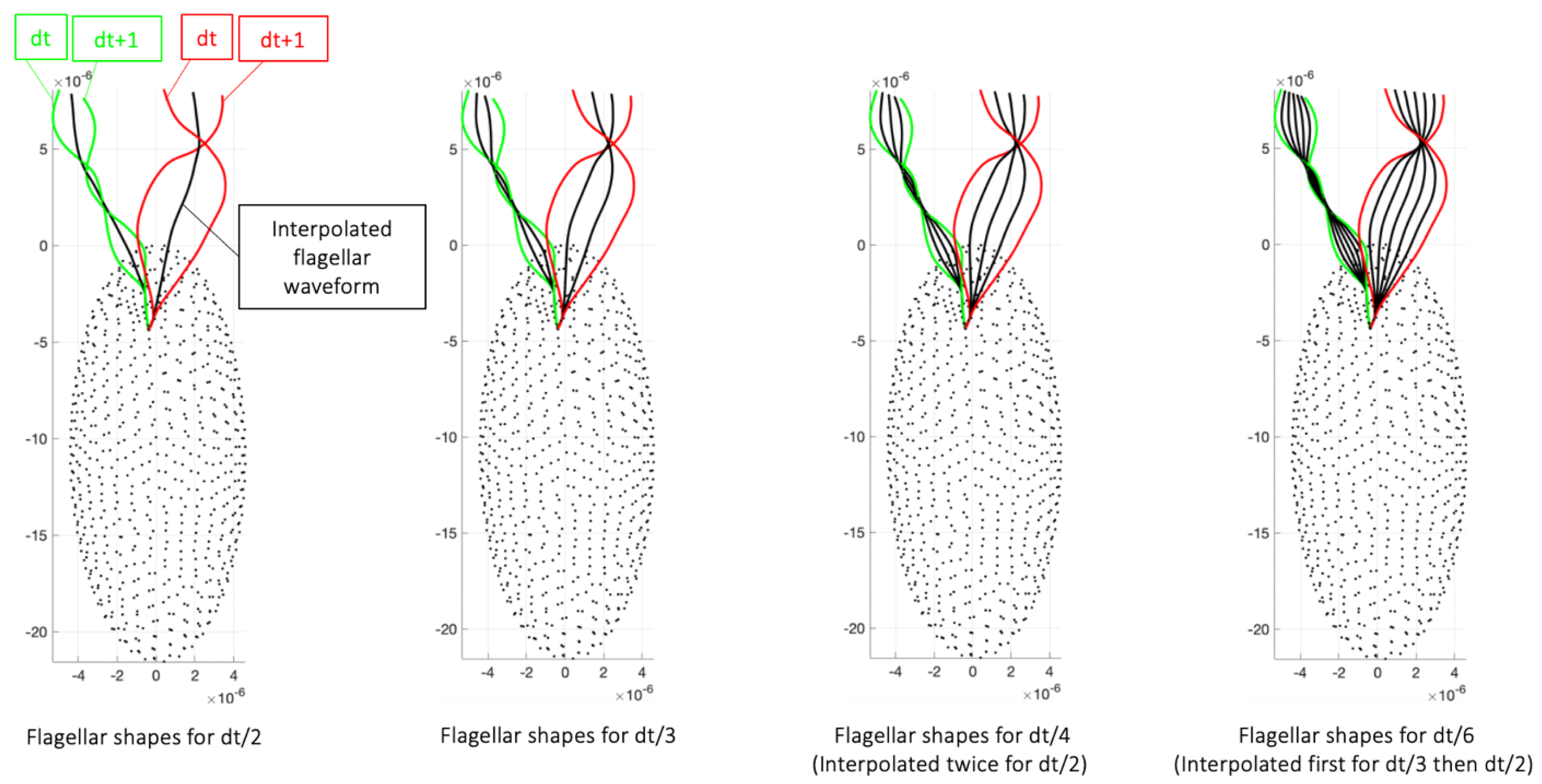
Appendix C. Convergence Study with Respect to Timestep Used in Simulation

While the high image-capture frequency of the video of interest (397 fps) allows for the observation of the periodic nature of propagated waves and the flagellar beating pattern of the individual reorienting cell, we conducted convergence studies to establish the reliability of our simulation results. These studies involved implementing smaller timesteps to ensure accurate resulting translational and rotational velocities. Furthermore, having smaller timesteps results in smaller velocities in between more predicted positions, hence yielding less jittery trajectories.
We used linear interpolation to determine the shape of the flagella between the captured waveforms. Specifically, we tracked the position of each Stokeslet on the flagella over time and computed an average of their positions between the initial timestep and the next one to interpolate their positions in between. Additionally, when needed, we interpolated new points at 1/3 and 2/3 along the resulting curve. This approach allowed us to predict the flagellar waveforms at smaller timesteps: dt/2, dt/3, dt/4, and dt/6 (see Figure A4).
To assess the convergence of our method, we first computed either the swimming velocity ( V ) or the angular velocity ( Ω ) at the different timesteps. Then, we used an average squared difference between the velocity values at the different timesteps and the most accurate values obtained at the finest time interval, dt/6, in order to calculate the error vector e α .
Figure A4. Illustration of the extrapolated flagellar waveforms at times t = dt/2, dt/3, dt/4 and dt/6.
Hydrobiology 03 00012 g0a4
This parameter serves as a quantitative measure of convergence over time, indicating how well the simulated values align with the most accurate results as the time interval decreases, thus providing insights into how accurately the method performs across various time intervals.
e α V = 1 N   d t ( V d t α V d t 6 ) 2   e α Ω = 1 N   d t ( Ω d t α Ω d t 6 ) 2
The α   subscript denotes the timestep divisor chosen, α = [ 1 ,   2 , 3 ,   4 ] . To analyze the convergence behavior of our output parameters, we plot the logarithm of the error vector e α   against the logarithm of the corresponding time interval d t α (Figure A5). The plots show that as we reduce the time intervals, the error decreases. The order of convergence is approximately 3 ( e α     ~   d t 3 ).
Figure A5. Error in translational and rotational velocity as a function of timestep.
Hydrobiology 03 00012 g0a5

References

  1. Lisicki, M.; Velho Rodrigues, M.F.; Goldstein, R.E.; Lauga, E. Swimming eukaryotic microorganisms exhibit a universal speed distribution. eLife 2019, 8, e44907. [Google Scholar] [CrossRef] [PubMed]
  2. Javornický, P.; Hindák, F. Cryptomonas frigoris spec. nova (Cryptophyceae), the new cyst-forming flagellate from the snow of the High Tatras. Biologia 1970, 25, 241–250. [Google Scholar] [PubMed]
  3. Klaveness, D. Ecology of the Cryptomonadida: A first review. In Growth and Reproductive Strategies of Freshwater Phytoplankton; Cambridge University Press: Cambridge, UK, 1988; pp. 105–133. [Google Scholar]
  4. Hill, D.R.A. A revised circumscription of Cryptomonas (Cryptophyceae) based on examination of Australian strains. Phycologia 1991, 30, 170–188. [Google Scholar] [CrossRef]
  5. Alcocer, J.; Lugo, A.; Sánchez, M.d.R.; Escobar, E. Isabela Crater-Lake: A Mexican insular saline lake. Hydrobiologia 1998, 381, 1–7. [Google Scholar] [CrossRef]
  6. Garibotti, I.; Vernet, M.; Ferrario, M.; Smith, R.; Ross, R.; Quetin, L. Phytoplankton Spatial Distribution Patterns along the Western Antarctic Peninsula (Southern Ocean). Mar. Ecol. Prog. Ser. 2003, 261, 21–39. [Google Scholar] [CrossRef]
  7. Hoef-Emden, K. Revision of the genus Cryptomonas (Cryptophyceae) II: Incongruences between the classical morphospecies concept and molecular phylogeny in smaller pyrenoid-less cells. Phycologia 2007, 46, 402–428. [Google Scholar] [CrossRef]
  8. Phlips, E.J.; Havens, K.E.; Lopes, M.R.M. Seasonal dynamics of phytoplankton in two Amazon flood plain lakes of varying hydrologic connectivity to the main river channel. Fundam. Appl. Limnol. 2008, 172, 99–109. [Google Scholar] [CrossRef]
  9. Hoef-Emden, K.; Archibald, J.M. Cryptophyta (Cryptomonads). In Handbook of the Protists; Archibald, J.M., Simpson, A.G.B., Slamovits, C.H., Eds.; Springer International Publishing: Cham, Switzerland, 2017; pp. 851–891. [Google Scholar] [CrossRef]
  10. Spaulding, S.A.; MCKnight, D.M.; Smith, R.L.; Dufford, R. Phytoplankton population dynamics in perennially ice-covered Lake Fryxell, Antarctica. J. Plankton Res. 1994, 16, 527–541. [Google Scholar] [CrossRef]
  11. Doust, A.B.; Wilk, K.E.; Curmi, P.M.G.; Scholes, G.D. The photophysics of cryptophyte light-harvesting. J. Photochem. Photobiol. Chem. 2006, 184, 1–17. [Google Scholar] [CrossRef]
  12. Spear-Bernstein, L.; Miller, K.R. Unique Location of the Phycobiliprotein Light-Harvesting Pigment in the Cryptophyceae. J. Phycol. 1989, 25, 412–419. [Google Scholar] [CrossRef]
  13. Moal, J.; Martin-Jezequel, V.; Harris, R.; Samain, J.-F.; Poulet, S. Interspecific and intraspecific variability of the chemical-composition of marine-phytoplankton. Oceanol. Acta 1987, 10, 339–346. [Google Scholar]
  14. Pedrós-Alió, C.; Massana, R.; Latasa, M.; Garcí-Cantizano, J.; Gasol, J.M. Predation by ciliates on a metalimnetic Cryptomonas population: Feeding rates, impact and effects of vertical migration. J. Plankton Res. 1995, 17, 2131–2154. [Google Scholar] [CrossRef]
  15. Weisse, T.; Kirchhoff, B. Feeding of the heterotrophic freshwater dinoflagellate Peridiniopsis berolinense on cryptophytes: Analysis by flow cytometry and electronic particle counting. Aquat. Microb. Ecol. 1997, 12, 153–164. [Google Scholar] [CrossRef]
  16. Roberts, E.C.; Laybourn-Parry, J. Mixotrophic cryptophytes and their predators in the Dry Valley lakes of Antarctica. Freshw. Biol. 1999, 41, 737–746. [Google Scholar] [CrossRef]
  17. Tirok, K.; Gaedke, U. Regulation of planktonic ciliate dynamics and functional composition during spring in Lake Constance. Aquat. Microb. Ecol. 2007, 49, 87–100. [Google Scholar] [CrossRef]
  18. Buma, A.G.J.; Treguer, P.; Kraay, G.W.; Morvan, J. Algal pigment patterns in different watermasses of the Atlantic sector of the Southern Ocean during fall 1987. Polar Biol. 1990, 11, 55–62. [Google Scholar] [CrossRef]
  19. Moline, M.A.; Claustre, H.; Frazer, T.K.; Schofield, O.; Vernet, M. Alteration of the food web along the Antarctic Peninsula in response to a regional warming trend. Glob. Change Biol. 2004, 10, 1973–1980. [Google Scholar] [CrossRef]
  20. Jeong, H.J.; Yoo, Y.D.; Lee, K.H.; Kim, T.H.; Seong, K.A.; Kang, N.S.; Lee, S.Y.; Kim, J.S.; Kim, S.; Yih, W.H. Red tides in Masan Bay, Korea in 2004–2005: I. Daily variations in the abundance of red-tide organisms and environmental factors. Harmful Algae 2013, 30, S75–S88. [Google Scholar] [CrossRef]
  21. Johnson, M.D.; Stoecker, D.K.; Marshall, H.G. Seasonal dynamics of Mesodinium rubrum in Chesapeake Bay. J. Plankton Res. 2013, 35, 877–893. [Google Scholar] [CrossRef]
  22. Piwosz, K.; Wiktor, J.M.; Niemi, A.; Tatarek, A.; Michel, C. Mesoscale distribution and functional diversity of picoeukaryotes in the first-year sea ice of the Canadian Arctic. ISME J. 2013, 7, 1461–1471. [Google Scholar] [CrossRef]
  23. Šupraha, L.; Bosak, S.; Ljubešić, Z.; Mihanović, H.; Olujić, G.; Mikac, I.; Viličić, D. Cryptophyte bloom in a Mediterranean estuary: High abundance of Plagioselmis cf. prolonga in the Krka River estuary (eastern Adriatic Sea). Sci. Mar. 2014, 78, 329–338. [Google Scholar] [CrossRef]
  24. Unrein, F.; Gasol, J.M.; Not, F.; Forn, I.; Massana, R. Mixotrophic haptophytes are key bacterial grazers in oligotrophic coastal waters. ISME J. 2014, 8, 164–176. [Google Scholar] [CrossRef] [PubMed]
  25. Yoo, Y.D.; Seong, K.A.; Jeong, H.J.; Yih, W.; Rho, J.-R.; Nam, S.W.; Kim, H.S. Mixotrophy in the marine red-tide cryptophyte Teleaulax amphioxeia and ingestion and grazing impact of cryptophytes on natural populations of bacteria in Korean coastal waters. Harmful Algae 2017, 68, 105–117. [Google Scholar] [CrossRef] [PubMed]
  26. Moran, J.; McKean, P.G.; Ginger, M.L. Eukaryotic Flagella: Variations in Form, Function, and Composition during Evolution. BioScience 2014, 64, 1103–1114. [Google Scholar] [CrossRef]
  27. Rossez, Y.; Wolfson, E.B.; Holmes, A.; Gally, D.L.; Holden, N.J. Bacterial Flagella: Twist and Stick, or Dodge across the Kingdoms. PLOS Pathog. 2015, 11, e1004483. [Google Scholar] [CrossRef] [PubMed]
  28. Namdeo, S.; Khaderi, S.N.; den Toonder, J.M.J.; Onck, P.R. Swimming direction reversal of flagella through ciliary motion of mastigonemes. Biomicrofluidics 2011, 5, 034108. [Google Scholar] [CrossRef] [PubMed]
  29. Liu, P.; Lou, X.; Wingfield, J.L.; Lin, J.; Nicastro, D.; Lechtreck, K. Chlamydomonas PKD2 organizes mastigonemes, hair-like glycoprotein polymers on cilia. J. Cell Biol. 2020, 219, e202001122. [Google Scholar] [CrossRef] [PubMed]
  30. Novarino, G. A companion to the identification of cryptomonad flagellates (Cryptophyceae = Cryptomonadea). Hydrobiologia 2003, 502, 225–270. [Google Scholar] [CrossRef]
  31. Kugrens, P.; Lee, R.E.; Andersen, R.A. Ultrastructural Variations in Cryptomonad Flagella. J. Phycol. 1987, 23, 511–518. [Google Scholar] [CrossRef]
  32. Morrall, S.; Greenwood, A.D. A comparison of the periodic substructure of the trichocysts of the Cryptophyceae and Prasinophyceae. Biosystems 1980, 12, 71–83. [Google Scholar] [CrossRef]
  33. Kugrens, P.; Clay, B.L. 21-CRYPTOMONADS. In Freshwater Algae of North America; Wehr, J.D., Sheath, R.G., Eds.; Aquatic Ecology; Academic Press: Cambridge, MA, USA, 2003; pp. 715–755. [Google Scholar] [CrossRef]
  34. Kugrens, P.; Lee, R.E. Ultrastructural Evidence for Bacterial Incorporation and Myxotrophy in the Photosynthetic Cryptomonad Chroomonas pochmanni Huber-Pestalozzi (Chyptomonadida). J. Protozool. 1990, 37, 263–267. [Google Scholar] [CrossRef]
  35. Brennen, C. Locomotion of Flagellates with Mastigonemes. J. Mechanochem. Cell Motil. 1976, 3, 207–217. [Google Scholar] [PubMed]
  36. Cahill, D.M.; Cope, M.; Hardham, A.R. Thrust reversal by tubular mastigonemes: Immunological evidence for a role of mastigonemes in forward motion of zoospores of Phytophthora cinnamomi. Protoplasma 1996, 194, 18–28. [Google Scholar] [CrossRef]
  37. Holwill, M.E.; Sleigh, M.A. Propulsion by hispid flagella. J. Exp. Biol. 1967, 10, 267–276. [Google Scholar] [CrossRef] [PubMed]
  38. Amador, G.J.; Wei, D.; Tam, D.; Aubin-Tam, M.-E. Fibrous Flagellar Hairs of Chlamydomonas reinhardtii Do Not Enhance Swimming. Biophys. J. 2020, 118, 2914–2925. [Google Scholar] [CrossRef] [PubMed]
  39. Kent, W.S. A Manual of the Infusoria: Including a Description of All Known Flagellate, Ciliate, and Tentaculiferous Protozoa, British and Foreign, and an Account of the Organization and the Affinities of the Sponges; David Bogue: Boca Raton, FL, USA, 1880; Volume 1. [Google Scholar]
  40. Pratt, D.M. The Phytoplankton of Narragansett Bay. Limnol. Oceanogr. 1959, 4, 425–440. [Google Scholar] [CrossRef]
  41. Jones, E.E. The Protozoa of Mobile Bay, Alabama; University of South Alabama: Mobile, AL, USA, 1974; pp. 1–113. [Google Scholar]
  42. Kevan, L. Hadrien Mary Kappa, GitHub Repository 2013. Available online: https://github.com/fiji/Kappa (accessed on 16 February 2024).
  43. Merk, A.; Bartesaghi, A.; Banerjee, S.; Falconieri, V.; Rao, P.; Davis, M.I.; Pragani, R.; Boxer, M.B.; Earl, L.A.; Milne, J.L.S.; et al. Breaking Cryo-EM Resolution Barriers to Facilitate Drug Discovery. Cell 2016, 165, 1698–1707. [Google Scholar] [CrossRef] [PubMed]
  44. Cortez, R. The Method of Regularized Stokeslets. SIAM J. Sci. Comput. 2001, 23, 1204–1225. [Google Scholar] [CrossRef]
  45. Cortez, R.; Fauci, L.; Medovikov, A. The method of regularized Stokeslets in three dimensions: Analysis, validation, and application to helical swimming. Phys. Fluids 2005, 17, 031504. [Google Scholar] [CrossRef]
  46. Flores, H.; Lobaton, E.; Méndez-Diez, S.; Tlupova, S.; Cortez, R. A study of bacterial flagellar bundling. Bull. Math. Biol. 2005, 67, 137–168. [Google Scholar] [CrossRef]
  47. Goto, T.; Masuda, S.; Terada, K.; Takano, Y. Comparison between Observation and Boundary Element Analysis of Bacterium Swimming Motion. JSME Int. J. Ser. C 2001, 44, 958–963. [Google Scholar] [CrossRef]
  48. Phan-Thien, N.; Tran-Cong, T.; Ramia, M. A boundary-element analysis of flagellar propulsion. J. Fluid Mech. 1987, 184, 533–549. [Google Scholar] [CrossRef]
  49. Ramia, M.; Tullock, D.L.; Phan-Thien, N. The role of hydrodynamic interaction in the locomotion of microorganisms. Biophys. J. 1993, 65, 755–778. [Google Scholar] [CrossRef] [PubMed]
  50. Shum, H.; Gaffney, E.; Smith, D. Modelling bacterial behaviour close to a no-slip plane boundary: The influence of bacterial geometry. R. Soc. Lond. Proc. Ser. A 2010, 466, 1725–1748. [Google Scholar] [CrossRef]
  51. Smith, D.J.; Gaffney, E.A.; Gadêlha, H.; Kapur, N.; Kirkman-Brown, J.C. Bend propagation in the flagella of migrating human sperm, and its modulation by viscosity. Cell Motil. Cytoskelet. 2009, 66, 220–236. [Google Scholar] [CrossRef] [PubMed]
  52. Martindale, J.D.; Jabbarzadeh, M.; Fu, H.C. Choice of computational method for swimming and pumping with nonslender helical filaments at low Reynolds number. Phys. Fluids 2016, 28, 021901. [Google Scholar] [CrossRef]
  53. Christensen, T. Algae: A Taxonomic Survey; AiO Tryk A/S: Odense, Denmark, 1980. [Google Scholar]
  54. Votta, J.J.; Jahn, T.L.; Griffith, D.L.; Fonseca, J.R. Nature of the Flagellar Beat in Trachelomonas volvocina, Rhabdomonas spiralis, Menoidium cultellus, and Chilomonas paramecium. Trans. Am. Microsc. Soc. 1971, 90, 404. [Google Scholar] [CrossRef] [PubMed]
  55. Manwell, R.D. Introduction to Protozoology; Dover Publications: New York, NY, USA, 1968. [Google Scholar]
  56. Bouck, G.B. The Structure, Origin, Isolation, and Composition of the Tubular Mastigonemes of the Ochromonas Flagellum. J. Cell Biol. 1971, 50, 362–384. [Google Scholar] [CrossRef] [PubMed]
  57. Das, P.; Mekonnen, B.; Alkhofash, R.; Ingle, A.V.; Workman, E.B.; Feather, A.; Zhang, G.; Chasen, N.; Liu, P.; Lechtreck, K.F. The Small Interactor of PKD2 protein promotes the assembly and ciliary entry of the Chlamydomonas PKD2–mastigoneme complexes. J. Cell Sci. 2024, 137, jcs261497. [Google Scholar] [CrossRef]
  58. Dai, J.; Ma, M.; Niu, Q.; Eisert, R.J.; Wang, X.; Das, P.; Lechtreck, K.F.; Dutcher, S.K.; Zhang, R.; Brown, A. Mastigoneme structure reveals insights into the O-linked glycosylation code of native hydroxyproline-rich helices. Cell 2024, 187, 1907–1921.e16. [Google Scholar] [CrossRef]
  59. Kage, A.; Omori, T.; Kikuchi, K.; Ishikawa, T. The shape effect of flagella is more important than bottom-heaviness on passive gravitactic orientation in Chlamydomonas reinhardtii. J. Exp. Biol. 2020, 223, jeb205989. [Google Scholar] [CrossRef]
  60. Jabbarzadeh, M.; Fu, H. A numerical method for inextensible elastic filaments in viscous fluids. J. Comput. Phys. 2020, 418, 109643. [Google Scholar] [CrossRef]
  61. Asadzadeh, S.S.; Walther, J.H.; Andersen, A.; Kiørboe, T. Hydrodynamic interactions are key in thrust-generation of hairy flagella. Phys. Rev. Fluids 2022, 7, 073101. [Google Scholar] [CrossRef]
  62. Asadzadeh, S.S.; Walther, J.H.; Kiørboe, T. Conflicting Roles of Flagella in Planktonic Protists: Propulsion, Resource Acquisition, and Stealth. PRX Life 2023, 1, 013002. [Google Scholar] [CrossRef]
Figure 1. Frame #1 of the reorientation event of interest (Supplementary Video S1). The growing arrows indicate the two possible longitudinal rotations of the cell body around the z-axis (counterclockwise in blue and clockwise in red), while the thin black arrow indicates its clockwise turning direction around the x-axis.
Hydrobiology 03 00012 g001
Figure 2. Workflow for simulating the motion of a simplified cell of C. paramecium bearing rigid mastigonemes.
Hydrobiology 03 00012 g002
Figure 3. SEM micrographs and measurements of C. paramecium. (AD) Examples of latero-ventral view showing gullet and flagella. (E) Corresponding box plots of dimensions. We measured the gullet’s dimensions from 19 images, of which the depth, length, and width could be measured in 9, 19, and 17 of the images, respectively. We measured the flagellar thickness in 25 images. The boxes represent the interquartile ranges (IQR), which are the ranges between the 25th and 75th percentiles. The whiskers indicate the smallest and largest values within 1.5 times the IQR from the lower and upper quartiles, respectively. The red lines in the box plots represent the mean of the measurements.
Hydrobiology 03 00012 g003
Figure 4. TEM micrographs and measurements of the mastigonemes of C. paramecium. (AC) Example TEM micrographs showing close-ups of the mastigonemes on the flagella. (D) Sketch of the flagella and mastigonemes. (E) Corresponding box plots of dimensions. The box plots are derived from 35 measurements of mastigoneme length and 34 measurements of the spacing between two adjacent mastigonemes. The boxes represent the interquartile ranges (IQR), which are the ranges between the 25th and 75th percentiles. The whiskers indicate the smallest and largest values within 1.5 times the IQR from the lower and upper quartiles, respectively. The red lines in the box plots represent the mean of the measurements.
Hydrobiology 03 00012 g004
Figure 5. Schematic of a C. paramecium showing the anatomical terms regarding the location and body axis. The flagella propel the cell with the swimming velocity V and angular velocity Ω .
Hydrobiology 03 00012 g005
Figure 6. Forward and backward motion of C. paramecium, observed in phase-contrast microscopy, with a high-speed camera recording at 85 fps. The red arrow indicates the direction of the cell swimming forward, while the blue arrow indicates the direction of the cell undergoing a reversion (Supplementary Video S6).
Hydrobiology 03 00012 g006
Figure 7. Reorientation event of interest (Supplementary Video S1). (A) Cell in Frame #1. The growing arrows indicate the two possible longitudinal rotations of the cell body around the z-axis (counterclockwise in blue and clockwise in red), while the thin black arrow indicates its clockwise turning direction around the x-axis necessary to rotate the cell body at a later time, such as in (B). (B) Cell in Frame #95. The less-active flagellum, indicated by the green label, and the active flagellum, indicated by the red label, play crucial roles in the cell’s movement.
Hydrobiology 03 00012 g007
Figure 8. Evolution of rotation angles over time. (A) Cell body turning angle around the x-axis. (B) Evolution of φ when the cell is initially presenting its ventral side to the observer; black: counterclockwise longitudinal rotation of the cell body needed to align the simulated flagella with their recorded shapes in the video; red: clockwise longitudinal rotation necessary to rotate the observed active flagellum back to the cell body frame; green: clockwise longitudinal rotation used to rotate the less-active flagellum back to the cell body frame. The less-active flagellum is observed only in frames 76–87, and those waveforms are looped over during the balance of the time of interest, using constant angles before and after frame 76–87 (see text). (C) Evolution of φ when the cell is initially presenting its dorsal side to the observer; black: clockwise longitudinal rotation of the cell body needed to align the simulated flagella with their recorded shapes in the video; red: counterclockwise longitudinal rotation necessary to rotate the observed active flagellum back to the cell body frame, green: counterclockwise longitudinal rotation used to rotate the less-active flagellum back to the cell body frame. The less-active flagellum is observed only in frames 76–87, and those waveforms are looped over during the balance the time of interest, using constant angles before and after frame 76–87 (see text).
Hydrobiology 03 00012 g008
Figure 9. Notation system. Each flagellum is characterized by a letter describing the mastigonemes configuration. The combination of two letters defines the overall arrangement case. (A) Configuration SS: smooth less-active flagellum and smooth active flagellum. (B) Configuration LR: mastigonemes oriented in the beating plane toward the left on the less-active flagellum and toward the right on the active flagellum. (C) Configuration TA: mastigonemes oriented in the plane perpendicular to the beating plane, toward the cell body on the active flagellum and away from the cell body on the active flagellum.
Hydrobiology 03 00012 g009
Figure 10. Comparison of experimental (in black) and simulated (SS in blue and RL in magenta) cell trajectories and orientations for ventrally presented cells. (A) Experimental cell trajectory, with its initial and final 3D positions. (B) SS cell trajectory, with its initial and final 3D positions. (C) RL cell trajectory, with its initial and final 3D positions. (D) Temporal evolution of the turning angles (experimental in black, SS in blue, and RL in magenta). (E) Temporal evolution of the longitudinal rotation angles (experimental in black, SS in blue and RL in magenta). (F) Temporal evolution of the net displacements of the apical point (experimental in black, SS in blue, and RL in magenta).
Hydrobiology 03 00012 g010
Figure 11. Temporal evolution of rotation angles (turning angle in (A) and longitudinal angle in (B)) and net displacement (C) compared with experimental data (blue) and with configuration “SS” (black) for a cell initially presenting ventrally. The blue shaded range indicates the uncertainties for the experimental data. Colored shaded ranges indicate uncertainties associated with each configuration (see text).
Hydrobiology 03 00012 g011
Figure 12. Temporal evolution of rotation angles (turning angle in (A) and longitudinal angle in (B)) and net displacement (C) compared with experimental data (blue) and with configuration “SS” (black) for a cell initially presenting dorsally. The blue shaded range indicates the uncertainties for the experimental data. Colored shaded ranges indicate uncertainties associated with each configuration (see text).
Hydrobiology 03 00012 g012
Table 1. Numerical values of parameters used in the discretization.
N i n i t i a l 100
D t 200 nm
d f active flagellum113 nm
d f less-active flagellum128 nm
N s t   on active flagellum41
N s t   on less-active flagellum48
N s t , m for 1.6 μm mastigonemes139
d m 11.5 nm
d c b 825 nm
ε a c t i v e   f l a g e l l u m 21.4 nm
ε l e s s   a c t i v e   f l a g e l l u m 21.4 nm
ε m a s t i g o n e m e s 11.5 nm
ε c e l l   b o d y 275.2 nm
Disclaimer/Publisher’s Note: The statements, opinions and data contained in all publications are solely those of the individual author(s) and contributor(s) and not of MDPI and/or the editor(s). MDPI and/or the editor(s) disclaim responsibility for any injury to people or property resulting from any ideas, methods, instructions or products referred to in the content.

