A Flexible Lifetime Distribution Based on Alpha Power Transformation: Properties, Inference and Data Analysis

Abstract

The Rayleigh–Logarithmic distribution provides a useful framework for modelling lifetime data by combining continuous lifetime variability with a logarithmic compounding mechanism. This study introduces a three-parameter Alpha Power Rayleigh–Logarithmic (APRL) distribution by applying the Alpha Power transformation to the classical Rayleigh–Logarithmic model. The additional transformation parameter allows the distributional shape, skewness, tail behaviour, and rate of increase in the hazard function to be adjusted while retaining the underlying structure of the baseline model. Several mathematical and reliability properties of the APRL distribution are derived, including the probability density and cumulative distribution functions, survival and hazard rate functions, quantile function, moments, order statistics, and mean residual life function. Model parameters are estimated by maximum likelihood using a multiple-start numerical optimization procedure, and the finite-sample performance of the estimators is investigated through Monte Carlo simulations under different parameter configurations and sample sizes. The simulation results show that estimation accuracy generally improves with increasing sample size, as reflected by decreasing bias, MSE, and RMSE, although estimation of the transformation parameter may exhibit greater variability for more extreme parameter settings. The practical performance of the APRL distribution is examined using the Aircraft Windshield Failure Times and Breaking Stress of Carbon Fibres datasets. Model comparisons based on information criteria, bootstrap-based goodness-of-fit assessment, and graphical diagnostics show that the APRL distribution provides competitive fits relative to several established lifetime distributions. In addition, mean time to failure and mean residual life analyses illustrate the practical interpretation of the reliability measures derived for the proposed model. Overall, the results support the APRL distribution as a useful alternative for the statistical analysis of lifetime and reliability data.

1. Introduction

The concept of symmetry plays a fundamental role in modern statistical modelling, reflecting balance, invariance, and proportional relationships among probabilistic structures. In probability theory, a distribution is regarded as symmetric when its probability density function is balanced around a central location, whereas many practical lifetime distributions exhibit varying degrees of asymmetry. The proposed Alpha Power Rayleigh–Logarithmic (APRL) distribution provides a flexible framework in which the shape parameter α regulates the degree of skewness and tail behaviour. As α varies, the distribution exhibits varying degrees of right-skewness and tail behaviour, allowing it to accommodate a wide range of lifetime data characteristics. Thus, rather than enforcing strict symmetry, the APRL distribution offers a continuous mechanism for modelling different levels of asymmetry. This flexibility makes the proposed model particularly suitable for representing lifetime data with different degrees of skewness, tail behaviour, and increasing failure rate characteristics.

It is seen that classical distributions are insufficient in data modelling in areas such as survival analysis, finance, and reliability theory. This problem has revealed the need for distributions to be more flexible for data modelling purposes. This requirement has increased the work on obtaining new probability distribution families by expanding the known distribution families. In addition to methods such as exponentiation, transformation, and parameter addition, “generative distributions” are commonly used to define new distribution families. Adamidis and Loukas [1] have given the two-parameter Exponential–Geometric (EG) distribution, which has a decreasing failure rate. Kus [2] introduced the Exponential–Poisson distribution (EP) and examined several of its characteristic properties. The Weibull–Poisson (WP) distribution, which generalized the EP distribution, was introduced by Lu and Shi [3]. Also, Binomial–Exponential 2 distribution is presented by Bakouch et al. [4].

Alpha Power transform is one of the methods for modelling daily life data, which makes distributions richer and more flexible. This method was proposed by Mahdavi and Kundu [5]. The aim is to add a skewness parameter to the baseline distribution. They studied various properties of one-parameter Exponential distribution, such as the moment generating function, order statistics, and entropy. The transformation has been applied by different researchers to obtain Alpha Power transformed distributions including Alpha Power transformed generalized Exponential distribution [6], on the Alpha Power Kumaraswamy distribution properties, simulation and application [7], Alpha Power transformed Lindley distribution [8], Alpha Power transformed Gombertz distribution [9], Alpha Power transformed log-logistic distribution [10], properties and applications of Alpha Power Weibull distribution [11], Alpha Power inverse Weibull distribution with reliability application [12], Alpha Power transformed Rayleigh distribution [13], Alpha Power Burr-XII distribution [14], Alpha Power inverted Exponential distribution [15], Alpha Power transformed extended Exponential distribution [16], etc. In addition, the subject of Alpha Power transformation has been researched by many other authors [17,18,19,20,21].

Recent studies have demonstrated the broad applicability of transformation-based distributional approaches in lifetime and reliability modelling. In particular, Alpha Power and related transformation mechanisms have been employed to extend several classical probability distributions, including the generalized Pareto, logistic, and Erlang distributions, as well as to construct bivariate models based on extreme shock mechanisms and broader Alpha Power-generated families. These studies have examined important statistical and reliability properties, parameter estimation procedures, simulation performance, and practical applications to real data. Related developments have also incorporated regression structures and mean residual life measures, further demonstrating the applicability of transformation-based models in lifetime and reliability analysis. Collectively, these contributions highlight the continuing interest in Alpha Power-based approaches for developing alternative probability models with useful statistical and reliability characteristics [22,23,24,25,26,27,28].

Despite these developments, several opportunities remain for extending transformation-based lifetime models. In particular, there is continuing scope for models that combine a compounding mechanism with an additional transformation parameter while retaining analytically tractable reliability characteristics and practical inferential procedures. Moreover, recent studies emphasize the importance of evaluating newly developed distributions not only through theoretical properties, but also through estimation performance, goodness-of-fit assessment, and reliability-oriented measures in real data applications. The present study addresses these opportunities by applying the Alpha Power transformation to the Rayleigh–Logarithmic distribution, thereby combining the logarithmic compounding structure of the baseline model with an additional transformation parameter. The resulting APRL model is investigated through its distributional and reliability properties, maximum likelihood estimation, Monte Carlo simulation, bootstrap-based inference and goodness-of-fit assessment, and real data applications. In addition, practical reliability measures, including MTTF and MRL, are evaluated for the fitted models to connect the theoretical development with reliability applications.

Let the probability density function $f\left(x\right)$ (pdf) and the cumulative distribution function be $F\left(x\right)$ (cdf) for a continuous random variable $X$. Mahdavi and Kundu [5] proposed a transformation called the Alpha Power with the pdf given as for $x\in R$:

$$f_{APT}\left(x\right)=\{\begin{array}{cc}{\displaystyle \frac{log\alpha }{\alpha -1}}f(x){\alpha }^{F\left(x\right)}& ,\alpha \in {\mathbb{R}}^{+}-\left\{1\right\}\\ f\left(x\right)& \alpha =1\end{array}$$

(1)

where ${\mathbb{R}}^{+}$ is the set of positive real numbers. The corresponding cdf is given as

$$F_{APT}\left(x\right)=\{\begin{array}{cc}{\displaystyle \frac{{\alpha }^{F\left(x\right)}-1}{\alpha -1}}& ,\alpha \in {\mathbb{R}}^{+}-\left\{1\right\}\\ F\left(x\right)& \alpha =1\end{array} .$$

(2)

The parameter α controls the effect of the Alpha Power transformation on the baseline distribution. When α = 1, the transformed model reduces to the original baseline distribution. Therefore, the APT family contains the baseline model as a special case and provides additional flexibility for modelling different distributional shapes.

The Alpha Power transformation (APT) of survival function $S_{APT}\left(x\right)$ and the hazard rate function $h_{APT}\left(x\right)$ are, respectively, given by

$$S_{APT}\left(x\right)=\{\begin{array}{cc}{\displaystyle \frac{\alpha }{\alpha -1}}\left(1-{\alpha }^{F\left(x\right)-1}\right),& \alpha \in {\mathbb{R}}^{+}-\left\{1\right\}\\ 1-F\left(x\right),& \alpha =1\end{array}$$

(3)

and

$$h_{APT}\left(x\right)=\{\begin{array}{cc}f(x){\displaystyle \frac{{\alpha }^{F\left(x\right)-1}}{1-{\alpha }^{F\left(x\right)-1}}}log\alpha ,& \alpha \in {\mathbb{R}}^{+}-\left\{1\right\}\\ {\displaystyle \frac{f\left(x\right)}{S\left(x\right)}},& \alpha =1\end{array}.$$

(4)

The survival function in Equation (3) represents the probability that the lifetime exceeds a specified value x, whereas the hazard rate in Equation (4) describes the instantaneous failure rate at time x. Through the transformation parameter α, the APT approach modifies the survival function and the rate of increase in the hazard function while preserving the basic structure of the baseline distribution.

The Rayleigh–Logarithmic (RL) distribution is widely used in reliability theory and survival analysis. This distribution plays an important role in real-life practice, including survival analysis, reliability theory, and ratio clinical studies. RL distribution has two parameters, shape (p) and scale (${\sigma }^2$). It is constructed as a distribution of independent Rayleigh random variable s when the sample size K has a logarithmic distribution member of continuous probability distribution and is considered as a model for failure time distribution. This distribution is one of the earliest in probability theory, and it was introduced by Bugatekin [29] and Hameed and Alwan [30].

RL distribution with parameters p and ${\sigma }^2$ with the probability density function and cumulative distribution function of a random variable $X$ are respectively given by

$$f\left(x\right)={\displaystyle \frac{-x}{{\sigma }^2\ln \left(1-p\right)}}{e}^{\left(-\frac{x^2}{2{\sigma }^2}\right)}.p.(1-p.e^{\left(-\frac{x^2}{2{\sigma }^2}\right)}{)}^{-1}, 0<p<1, {\sigma }^2>0$$

and

$$F\left(x\right)=1-{\displaystyle \frac{In\left(1-{p.e}^{\left(-\frac{x^2}{2{\sigma }^2}\right)}\right)}{In\left(1-p\right)}} .$$

Here, p is the shape parameter and ${\sigma }^2$ is the scale parameter of the RL distribution. The parameter p mainly controls the shape and tail behavior of the distribution, while ${\sigma }^2$ determines the overall scale of the lifetime observations. These two parameters allow the RL distribution to represent different lifetime patterns encountered in reliability and survival studies.

Bugatekin made comparisons with other mixed distributions using a real dataset in her article in 2017. Accordingly, the RL distribution was found to be a good competitor to the Binomial–Exponential 2 (BE2), two-parameter Weibull (W), Exponentiated–Exponential (EE), Weighted–Exponential (WE) and Poisson–Exponential (PE) distributions.

The Rayleigh–Logarithmic (RL) distribution provides a useful compound lifetime model by combining continuous lifetime behaviour with a logarithmic counting mechanism. Owing to this compound structure, it has demonstrated satisfactory performance in modelling heterogeneous lifetime data. Nevertheless, the original RL distribution contains only two parameters, which may limit its ability to accommodate the diverse levels of skewness, tail behaviour, and increasing hazard rate characteristics encountered in practical reliability and survival studies. Consequently, there remains a need for a more flexible extension capable of preserving the advantages of the RL model while improving its adaptability to complex lifetime data.

Although numerous Alpha Power transformed distributions have been proposed in the literature, most are constructed from relatively simple baseline models such as the Exponential, Rayleigh, Weibull, Lindley, and Burr XII distributions. In contrast, the proposed APRL distribution is developed from the Rayleigh–Logarithmic distribution, which is itself a compound lifetime model. As a result, the proposed model combines two complementary modelling mechanisms: the logarithmic compounding structure inherited from the RL distribution and the additional flexibility introduced by the Alpha Power transformation. This combination enables the APRL distribution to accommodate heterogeneous lifetime patterns while providing greater control over skewness, tail behaviour, and the rate of increase in the hazard function than either the original RL distribution or existing Alpha Power models based on simpler parent distributions. Consequently, unlike the APR and RL distributions, the proposed APRL model simultaneously preserves the compound lifetime structure of the RL distribution and introduces additional flexibility through the Alpha Power transformation, resulting in improved control over skewness, tail behaviour, and hazard rate characteristics.

The additional Alpha Power parameter is introduced to enhance the statistical flexibility of the model rather than to represent a specific physical failure mechanism. From a modelling perspective, this parameter governs the shape of the distribution by regulating its skewness, tail behaviour, and the rate of increase in the hazard function, thereby allowing the model to accommodate a broad range of lifetime data characteristics. In practical reliability and survival applications, these features often reflect unobserved heterogeneity, population variability, and latent risk factors that cannot always be adequately captured by the baseline model. Consequently, the proposed APRL distribution provides a parsimonious yet flexible framework for modelling complex lifetime data while preserving the underlying probabilistic structure of the original Rayleigh–Logarithmic distribution.

Motivated by these observations, this study proposes a new three-parameter Alpha Power Rayleigh–Logarithmic (APRL) distribution by incorporating the Alpha Power transformation into the classical RL distribution. The additional shape parameter considerably enhances the flexibility of the model while preserving the attractive characteristics of the original compound distribution. Consequently, the proposed model provides greater control over skewness, tail behaviour, and increasing hazard rate characteristics, making it suitable for modelling a wide variety of lifetime data encountered in reliability and survival analysis. Several fundamental mathematical properties of the APRL distribution, including its probability density function, cumulative distribution function, quantile function, moments, and mean residual life function, are derived. Statistical inference is developed using the maximum likelihood method, and the finite-sample performance of the estimators is investigated through extensive Monte Carlo simulations. Finally, the practical usefulness of the proposed model is demonstrated through comprehensive real data applications and comparisons with closely related lifetime distributions.

2. Alpha Power Rayleigh–Logarithmic (APRL) Distribution

2.1. Distributions

In this study, a new distribution called Alpha Power RL distribution (APRL) is proposed by using the Alpha Power conversion method and the RL distribution. Let $\phi =(\alpha ,p,{\sigma }^2{)}^T$. From (1), the random variable $X$ is said to have a three-parameter APRL distribution with the scale parameter ${\sigma }^2>0$ and shape parameters $\alpha >0$ and $0<p<1$, if the pdf of $x>0$ is

$$f_{APRL}\left(x,\phi \right)={\displaystyle \frac{-\log \alpha }{\left(\alpha -1\right){\sigma }^2\ln \left(1-p\right)}}x{e}^{\left(-{\displaystyle \frac{x^2}{2{\sigma }^2}}\right)}.p.(1-p.e^{\left(-{\displaystyle \frac{x^2}{2{\sigma }^2}}\right)}{)}^{-1}{\alpha }^{1-{\displaystyle \frac{\ln \left(1-{p.e}^{\left(-\frac{x^2}{2{\sigma }^2}\right)}\right)}{\ln \left(1-p\right)}}}, \alpha \in {\mathbb{R}}^{+}-\left\{1\right\},x>0$$

(5)

and the corresponding cdf is

$$F_{APRL}\left(x,\phi \right)={\displaystyle \frac{{\alpha }^{1-\frac{\ln \left(1-{p.e}^{\left(-\frac{x^2}{2{\sigma }^2}\right)}\right)}{\ln \left(1-p\right)}}}{\alpha -1}}-1, \alpha \in {\mathbb{R}}^{+}-\left\{1\right\},x>0.$$

(6)

The probability density function in Equation (5) defines the distribution of the lifetime variable, while Equation (6) gives the corresponding cumulative distribution function. The additional parameter α introduced through the Alpha Power transformation provides extra flexibility beyond the baseline RL distribution by allowing different distributional shapes without changing the support of the model.

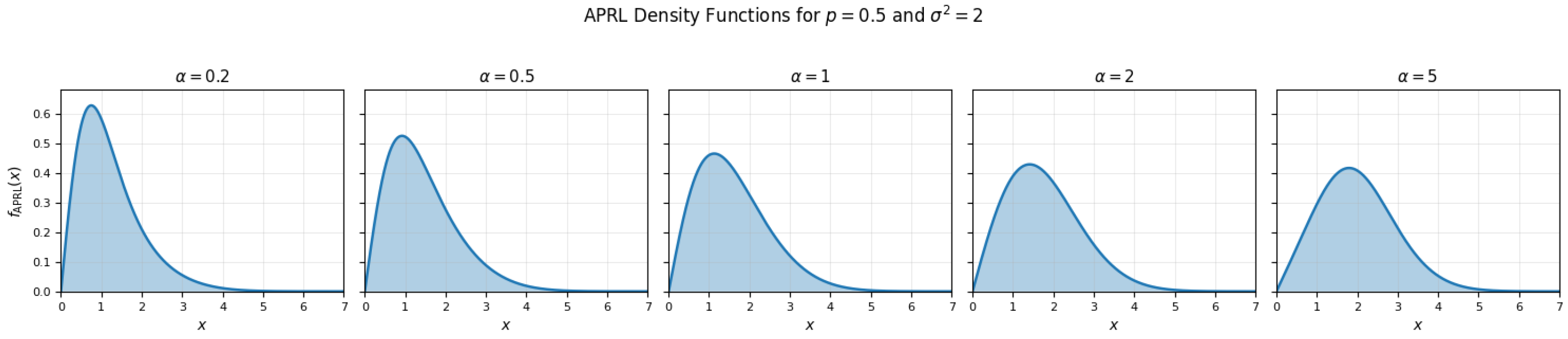
As the parameter α increases in the APRL distribution, the shape of the distribution changes significantly. For small α values (e.g., $\alpha =1.1$), the distribution is highly peaked and right-skewed, with the highest density occurring at small x values and a short tail. When α is 2 or 5, the peak shifts to the right, the distribution becomes more spread out, and the tails grow thicker. At $\alpha =10$, the skewness is reduced, and the distribution begins to take on a more balanced and nearly symmetric shape. For larger values such as $\alpha =20$, the distribution becomes flatter and more widely spread, and the peak becomes less prominent. Therefore, as α increases, the APRL distribution becomes more dispersed, less skewed, and exhibits longer tails.

In Figure 1, the histograms of the APRL distribution and the corresponding theoretical pdf curves are shown for different α values. The results indicate that the shape of the distribution changes noticeably as α increases. For small α values, the distribution is more spread out and right-skewed, whereas for larger α values, the peak shifts to the left and the distribution becomes more concentrated around smaller values. Additionally, the close agreement between the theoretical pdf curves and the sample histograms demonstrates that the sampling method accurately represents the APRL distribution.

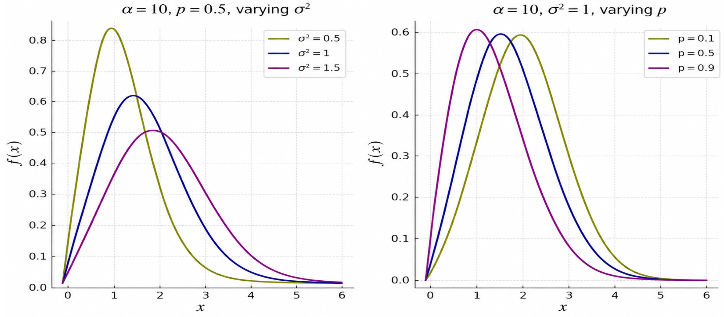
Figure 2 illustrates the probability density function of the APRL distribution under different parameter configurations, showing the effects of varying ${\sigma }^2$ and p while keeping the remaining parameters fixed.

2.2. Special Case

The proposed APRL distribution includes the classical Rayleigh–Logarithmic (RL) distribution as a limiting case. To verify this property, consider the cumulative distribution function of the APRL distribution,

$$F\left(x,\phi \right)={\displaystyle \frac{{\alpha }^{G\left(x\right)}-1}{\alpha -1}}$$

where $G\left(x\right)$ denotes the cumulative distribution function of the Rayleigh–Logarithmic distribution.

As $\alpha \to 1$, both the numerator and denominator converge to zero, yielding an indeterminate form of type 0/0. Applying L’Hospital’s rule gives

$$\underset{\alpha \to 1}{\lim }F\left(x,\phi \right)=\underset{\alpha \to 1}{\mathrm{l}\mathrm{i}\mathrm{m}}{\displaystyle \frac{\partial }{\partial \alpha }}\left({\alpha }^{G\left(x\right)}-1\right)=\underset{\alpha \to 1}{\mathrm{l}\mathrm{i}\mathrm{m}}G\left(x\right){\alpha }^{G\left(x\right)}-1=G(x)$$

Hence,

$$\underset{\alpha \to 1}{\mathrm{l}\mathrm{i}\mathrm{m}}F\left(x,\phi \right)=G\left(x\right)=F_{RL}\left(x\right).$$

Similarly, the probability density function of the APRL distribution is

$$f\left(x,\phi \right)={\displaystyle \frac{\ln \left(\alpha \right)}{\alpha -1}}{\alpha }^{G\left(x\right)}g(x)$$

where $g(x)$ is the probability density function of the Rayleigh–Logarithmic distribution. Using the limits

$$\underset{\alpha \to 1}{\mathrm{l}\mathrm{i}\mathrm{m}}{\displaystyle \frac{\ln \left(\alpha \right)}{\alpha -1}}=1, \underset{\alpha \to 1}{\mathrm{l}\mathrm{i}\mathrm{m}}{\alpha }^{G\left(x\right)}=1$$

it immediately follows that

$$\underset{\alpha \to 1}{\mathrm{l}\mathrm{i}\mathrm{m}}f\left(x,\phi \right)=g\left(x\right)=f_{RL}\left(x\right).$$

Therefore, the proposed APRL distribution constitutes a genuine extension of the classical Rayleigh–Logarithmic distribution, with the RL model recovered as the limiting case when $\alpha \to 1$.

3. Characteristic Structure of the APRL Distribution

3.1. Survival and Hazard Rate Functions

The life function is the function that shows the probability distribution of lifetimes. The survival function can be expressed as $S\left(x\right)=1-F\left(x\right)$, and the survival function of the APRL distribution obtained using this equation is as follows:

$$S_{APRL}\left(x,\phi \right)={\displaystyle \frac{\alpha }{\alpha -1}}(1-{\alpha }^{{\displaystyle \frac{-\ln \left(1-{p.e}^{\left(-\frac{x^2}{2{\sigma }^2}\right)}\right)}{\ln \left(1-p\right)}}}), \alpha \in {\mathbb{R}}^{+}-\left\{1\right\},x>0.$$

The hazard function is obtained as $h\left(x\right)=f\left(x\right)/S\left(x\right)$ and the hazard function of the APRL distribution can be written as

$$h_{APRL}\left(x,\phi \right)={\displaystyle \frac{-{\alpha }^{\frac{-\ln \left(1-p.e^{\left(-\frac{x^2}{2{\sigma }^2}\right)}\right)}{\ln \left(1-p\right)}}}{1-{\alpha }^{\frac{-\ln \left(1-{p.e}^{\left(-\frac{x^2}{2{\sigma }^2}\right)}\right)}{\ln \left(1-p\right)}}}}{\displaystyle \frac{x}{{\sigma }^2\ln \left(1-p\right)}}{e}^{\left(-{\displaystyle \frac{x^2}{2{\sigma }^2}}\right)}.p.(1-{p.e}^{\left(-{\displaystyle \frac{x^2}{2{\sigma }^2}}\right)}{)}^{-1}log\alpha , \alpha \in {\mathbb{R}}^{+}-\left\{1\right\}.$$

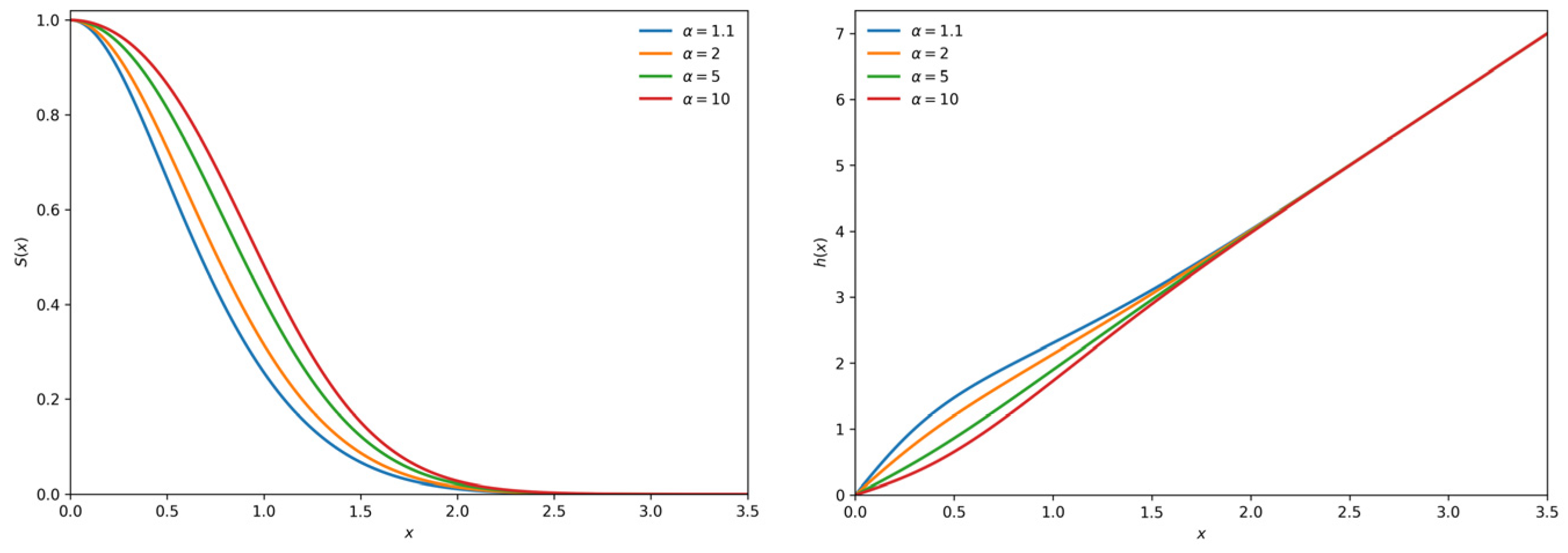
Figure 3 shows the survival and hazard rate functions of the APRL distribution for different values of the shape parameter α. As ${\sigma }^2$ varies, both functions exhibit different reliability and failure rate behaviours, demonstrating the flexibility of the proposed model.

3.2. Mean Residual Life Function

The mean residual life (MRL) function is an important reliability characteristic that describes the expected remaining lifetime of a component given that it has survived up to time x. It is widely used in reliability engineering, survival analysis, and risk assessment to evaluate the ageing behaviour of lifetime distributions. For a non-negative random variable X, the MRL function is defined as

$$m\left(x\right)=E\left(X-x\right|X>x),$$

which can be expressed as $S\left(t\right)$ denotes the survival function of the APRL distribution.

Substituting the survival function given in Section 3.1 yields

$$m\left(x\right)={\displaystyle \frac{1}{S_{APRL}\left(x\right)}}{\int }_x^{\infty }\left[1-{\displaystyle \frac{{\alpha }^{G_{RL}\left(t\right)}-1}{\alpha -1}}\right]dt,$$

where

$$G_{RL}\left(t\right)=1-{\displaystyle \frac{\ln \left(1-{p.e}^{\left(-\frac{x^2}{2{\sigma }^2}\right)}\right)}{\ln \left(1-p\right)}}.$$

Since the above integral does not generally admit a closed-form solution, the mean residual life function is evaluated numerically for specified values of $\alpha$, $p$, and ${\sigma }^2$. For the numerical illustrations presented in this study, the integral was evaluated using the adaptive quadrature algorithm implemented in the integrate() function in R, which provides reliable numerical approximations with built-in error control.

The MRL function provides valuable insight into the ageing characteristics of the proposed distribution. Depending on the parameter values, the APRL model can exhibit different remaining lifetime behaviours, demonstrating its flexibility for modelling a wide variety of lifetime data arising in reliability and survival applications.

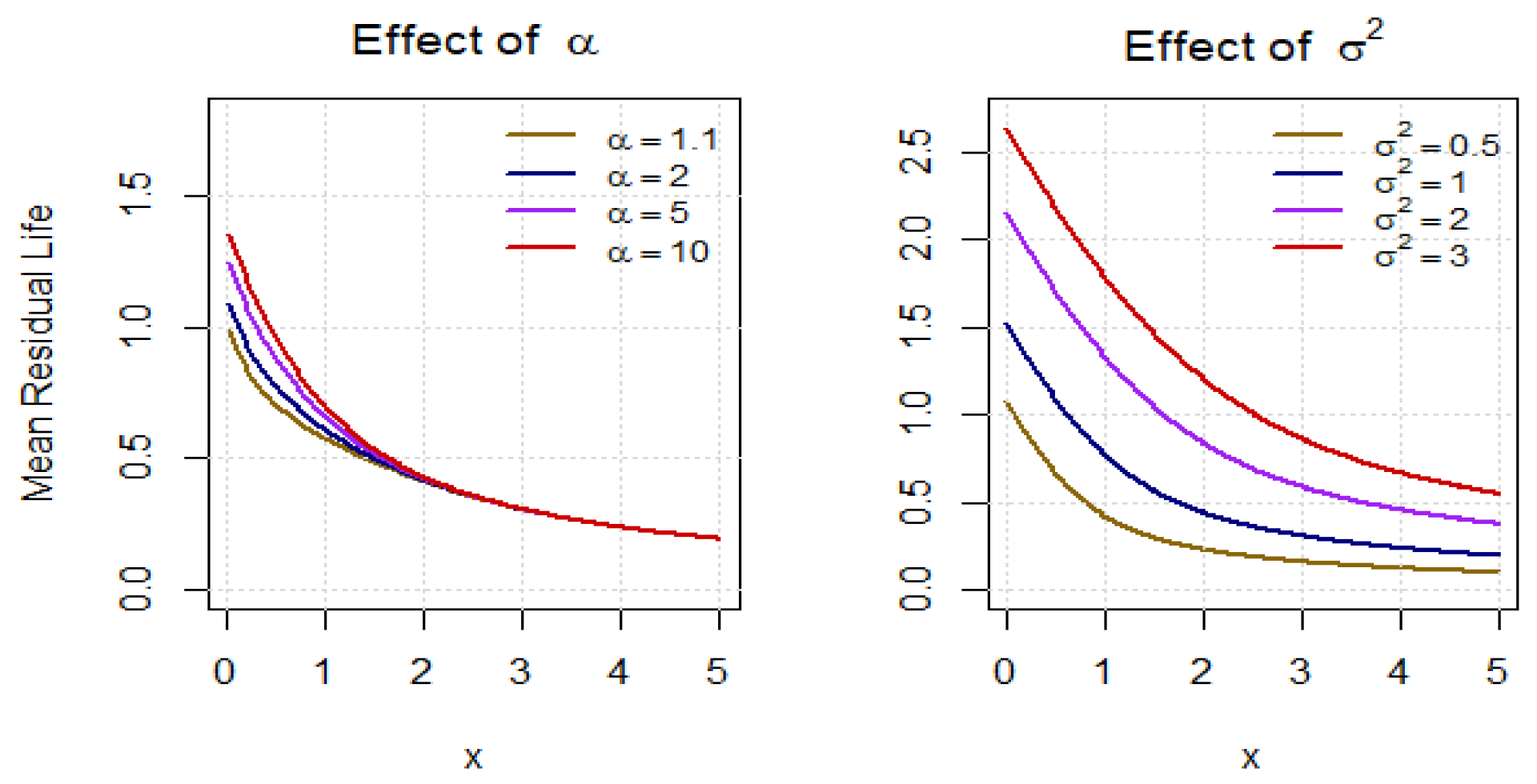
Figure 4 illustrates the effects of the shape parameter $\alpha$ and the scale parameter ${\sigma }^2$ on the mean residual life (MRL) function of the proposed APRL distribution. Since the principal contribution of the proposed model lies in the introduction of the additional Alpha Power parameter α, its influence on the remaining lifetime behavior is examined in the left panel. The right panel illustrates the effect of the scale parameter ${\sigma }^2$, which governs the overall lifetime scale of the distribution. It can be observed that larger values of p increase the initial mean residual life, whereas the differences among the curves gradually diminish as the survival time increases. In contrast, increasing ${\sigma }^2$ results in consistently larger expected remaining lifetimes over the entire support. These findings demonstrate that the proposed APRL distribution provides considerable flexibility in modelling different remaining lifetime behaviors encountered in reliability and survival analysis.

3.3. Moments

Since 0 < p < 1, 0 < ${\sigma }^2$ < 1, and $\alpha >0$, the infinite series appearing in the density expansion is absolutely convergent. Therefore, the series representation converges for all x > 0.

The k-th moment of the APRL distribution is given by

$$E\left(X^k\right)={\int }_0^{\infty }{x}^k. f_{APRL}\left(x,\phi \right)dx,$$

Using

$${\alpha }^{{\displaystyle \frac{-\ln \left(1-{p.e}^{\left(-\frac{x^2}{2{\sigma }^2}\right)}\right)}{\ln \left(1-p\right)}}}={\left(1-{p.e}^{\left(-{\displaystyle \frac{x^2}{2{\sigma }^2}}\right)}\right)}^{{\displaystyle \frac{-ln\alpha }{\mathrm{l}\mathrm{n}\left(1-p\right)}}},$$

the density can be expressed in a form involving

$${\left(1-{p.e}^{\left(-{\displaystyle \frac{x^2}{2{\sigma }^2}}\right)}\right)}^{-\beta },$$

where

$$\beta =1+{\displaystyle \frac{ln\alpha }{\mathrm{l}\mathrm{n}\left(1-p\right)}}$$

Let $y=e^{\left(-{\displaystyle \frac{x^2}{2{\sigma }^2}}\right)}$. Then

$$x=\sqrt{-2{\sigma }^{2}lny}, {\displaystyle \frac{x}{{\sigma }^2}}{e}^{\left(-{\displaystyle \frac{x^2}{2{\sigma }^2}}\right)}dx=-dy$$

and the integration limits x = 0 and $x\to \infty$ correspond to y = 1 and y = 0, respectively. Therefore,

$$E\left(X^k\right)={\displaystyle \frac{\alpha p(-ln\alpha )}{\left(\alpha -1\right)\mathrm{l}\mathrm{n}(1-p)}}{2}^{k/2}{\left({\sigma }^2\right)}^{{\displaystyle \frac{k}{2}}}{\int }_0^1{\left(-lny\right)}^{{\displaystyle \frac{k}{2}}}{(1-py)}^{-\beta }dy.$$

For $0<x<1$ and $0\le y\le 1$, one has $\left|py\right|\le p<1$. Hence, the generalized binomial expansion

$${\left(1-py\right)}^{-\beta }={\displaystyle \sum _{n=0}^{\infty }}{\displaystyle \frac{{\left(\beta \right)}_n}{n!}}{p}^n{y}^n$$

is absolutely and uniformly convergent $[0,1]$, where ${\left(\beta \right)}_n$ denotes the Pochhammer symbol. In particular,

$${\displaystyle \sum _{n=0}^{\infty }}\left|{\displaystyle \frac{{\left(\beta \right)}_n}{n!}}{p}^n{y}^n\right|\le {\displaystyle \sum _{n=0}^{\infty }}\left|{\displaystyle \frac{{\left(\beta \right)}_n}{n!}}\right|p^n<\infty .$$

Moreover, the weighting function ${\left(-lny\right)}^{{\displaystyle \frac{k}{2}}}$ is integrable over (0,1) for k > −2. Thus, the expanded integrand is dominated by an integrable function. Consequently, the order of summation and integration may be interchanged by the dominated convergence theorem. It follows that

$$E\left(X^k\right)={\displaystyle \frac{\alpha p(-ln\alpha )}{\left(\alpha -1\right)\mathrm{l}\mathrm{n}(1-p)}}{2}^{k/2}{\left({\sigma }^2\right)}^{{\displaystyle \frac{k}{2}}}{\displaystyle \sum _{n=0}^{\infty }}{\displaystyle \frac{{\left(\beta \right)}_n}{n!}}{p}^n{\int }_0^1{y}^n{\left(-lny\right)}^{{\displaystyle \frac{k}{2}}}dy.$$

Using the identity

$${\int }_0^1{y}^n{\left(-lny\right)}^{m}dy={\displaystyle \frac{\Gamma (m+1)}{{(n+1)}^{m+1}}}.$$

With $m=k/2$, the k-th raw moment becomes

$$E\left(X^k\right)=\alpha p{\sigma }^k{\displaystyle \frac{-ln\alpha }{\left(\mathsf{\alpha }-1\right)\ln \left(1-p\right)}}{2}^{{\displaystyle \frac{k}{2}}} \Gamma \left({\displaystyle \frac{k}{2}}+1\right){\displaystyle \sum _{n=0}^{\infty }}{\displaystyle \frac{{\left(\beta \right)}_n}{n!}}{\displaystyle \frac{p^n}{{\left(n+1\right)}^{\frac{k}{2}+1}}}$$

The above expression provides a unified representation of all raw moments of the APRL distribution. Consequently, important descriptive measures such as the mean and variance can be obtained directly by substituting the appropriate values of k into the general formula.

From this general formula:

The mean is obtained by setting k = 1:

$$E\left(X\right)=\alpha p\sigma {\displaystyle \frac{-ln\alpha }{(\mathsf{\alpha }-1)\mathrm{l}\mathrm{n}(1-p)}}\sqrt{2} \Gamma ({\displaystyle \frac{3}{2}}){\displaystyle \sum _{n=0}^{\infty }}{\displaystyle \frac{{\left(\beta \right)}_n}{n!}}{\displaystyle \frac{p^n}{{(n+1)}^{\frac{3}{2}}}}$$

The second moment is obtained by setting k = 2:

$$E\left(X^2\right)=\alpha p{\sigma }^2{\displaystyle \frac{-ln\alpha }{(\mathsf{\alpha }-1)\mathrm{l}\mathrm{n}(1-p)}}2 \Gamma (2){\displaystyle \sum _{n=0}^{\infty }}{\displaystyle \frac{{\left(\beta \right)}_n}{n!}}{\displaystyle \frac{p^n}{{(n+1)}^2}}$$

The variance is then

$$V\left(X\right)=E\left(X^2\right)-{\left[E\left(X\right)\right]}^2$$

The computed values of the mean, variance, skewness, and kurtosis for the selected parameter sets are presented below.

The numerical characteristics reported in

Table 1. Numerical results for the mean, variance, skewness, and kurtosis under selected parameter settings.

p, σ2, α	Mean	Variance	Skewness	Kurtosis
(0.7,0.5,2)	0.8235	0.2081	0.7339	3.4066
(0.6,1.0,3)	1.2853	0.4329	0.5962	3.1990
(0.9,0.8,5)	1.0233	0.3371	0.7455	3.3991
(0.5,1.2,8)	1.6347	0.5277	0.4035	3.0498
(0.8,0.7,10)	1.1416	0.3024	0.5278	3.1482

were obtained by direct numerical integration of the corresponding raw moments using the adaptive quadrature algorithm implemented in the integrate() function in R. Relative and absolute error tolerances were both set to ${10}^{-10}$, and therefore no truncation of infinite series was required.

The numerical characteristics reported in Table 1 were obtained by direct numerical integration of the corresponding raw moments using the same adaptive quadrature procedure described above. The results demonstrate that the distributional characteristics of the APRL model are substantially influenced by the model parameters. As expected, the mean and variance vary according to the combined effects of $\alpha$, $p$, and ${\sigma }^2$, reflecting changes in both the location and dispersion of the distribution. The transformation parameter α also has a noticeable effect on the shape of the distribution. For the parameter combinations considered, the skewness values remain positive, indicating that the APRL distribution preserves a right-skewed structure, while their magnitudes vary across different parameter settings, illustrating the flexibility of the proposed model in representing different degrees of asymmetry. Likewise, the kurtosis values range from approximately 3.05 to 3.41, indicating that the tail behaviour can vary from nearly mesokurtic to moderately heavy-tailed depending on the parameter configuration. Overall, these findings confirm that the interaction among the model parameters provides considerable flexibility in controlling the location, dispersion, asymmetry, and tail behaviour of the proposed APRL distribution.

3.4. Quantile Function of the APRL Distribution

For the APRL distribution, the quantile function $Q\left(u\right)$ can be written as

$$Q_u\left(u\right)=\sigma \sqrt{-2ln\left({\displaystyle \frac{1-(1-p){[1+u\left(\alpha -1\right)]}^{\frac{-\mathrm{l}\mathrm{n}(1-p)}{ln\alpha }}}{p}}\right)}, 0<u<1$$

The quantile function provides a convenient basis for deriving quantile-based descriptive measures. In particular, Bowley’s skewness and Moor’s kurtosis are computed from selected quantiles and provide robust measures of distributional shape that are less sensitive to extreme observations than conventional moment-based measures.

The random variable X’s 25th and 75th percentiles are determined as

$$Q_1=Q_{0.25}=\sigma \sqrt{-2ln\left({\displaystyle \frac{1-(1-p){[1+0.25\left(\alpha -1\right)]}^{\frac{-\mathrm{l}\mathrm{n}(1-p)}{ln\alpha }}}{p}}\right)}$$

$$Q_3=Q_{0.75}=\sigma \sqrt{-2ln\left({\displaystyle \frac{1-(1-p){[1+0.75\left(\alpha -1\right)]}^{\frac{-\mathrm{l}\mathrm{n}(1-p)}{ln\alpha }}}{p}}\right)}$$

The quantile function yields the Bowley’s skewness as

$$S_k={\displaystyle \frac{Q_{0.75}-2Q_{0.50}+Q_{0.25}}{Q_{0.75}-Q_{0.25}}}$$

The kurtosis of the Moor is represented as

$$M_k={\displaystyle \frac{Q_{0.875}-Q_{0.625}-Q_{0.375}+Q_{0.125}}{Q_{0.75}-Q_{0.25}}}$$

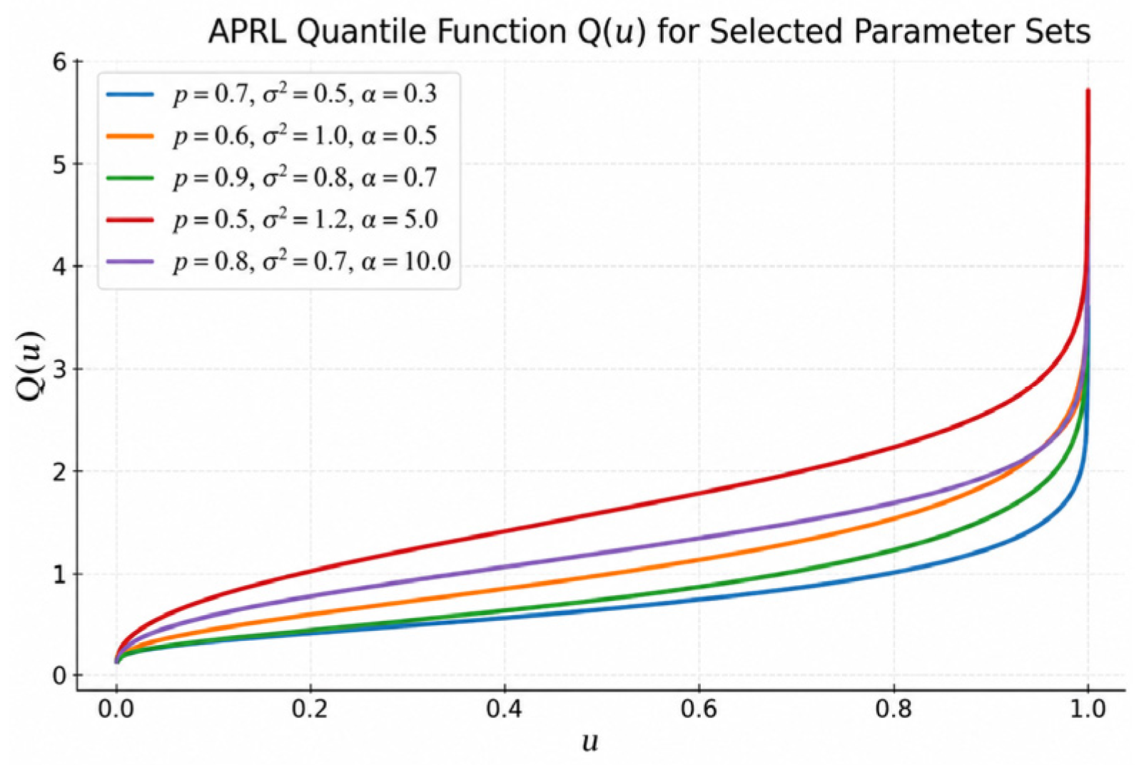
Figure 5 illustrates how the quantile function of the APRL distribution responds to changes in the parameters $p$, ${\sigma }^2$, and $\alpha$. As the parameter values increase, the quantile curves shift upward, indicating that larger values are produced for the same probability level. In particular, the steeper rise in the curve near $u\to 1$ for larger $\alpha$ values shows that the upper tail of the distribution is strongly governed by $\alpha$. In addition, the monotonic increase in all curves is consistent with the typical behaviour of quantile functions. Overall, these results demonstrate that the tail behaviour and spread of the APRL distribution are highly flexible and strongly influenced by its parameters.

Table 2. Results of some numerical values of $Q_1$, median ($Q_2)$, $Q_3$, $S_k$ and $M_k$ for various parameter settings.

$\mathit{p}, {\mathit{\sigma }}^2,$ $\mathit{\alpha }$	${\mathit{Q}}_1$	Median	${\mathit{Q}}_3$	${\mathit{S}}_{\mathit{k}}$	${\mathit{M}}_{\mathit{k}}$
0.35, 0.4, 0.4	0.3572	0.5755	0.8593	0.1304	0.3417
0.55, 0.9, 0.8	0.5694	0.9192	1.3666	0.1216	0.3148
0.75, 1.5, 2.5	0.8326	1.3269	1.9253	0.0952	0.2512
0.85, 0.6, 6	0.5738	0.8967	1.2754	0.0793	0.2136
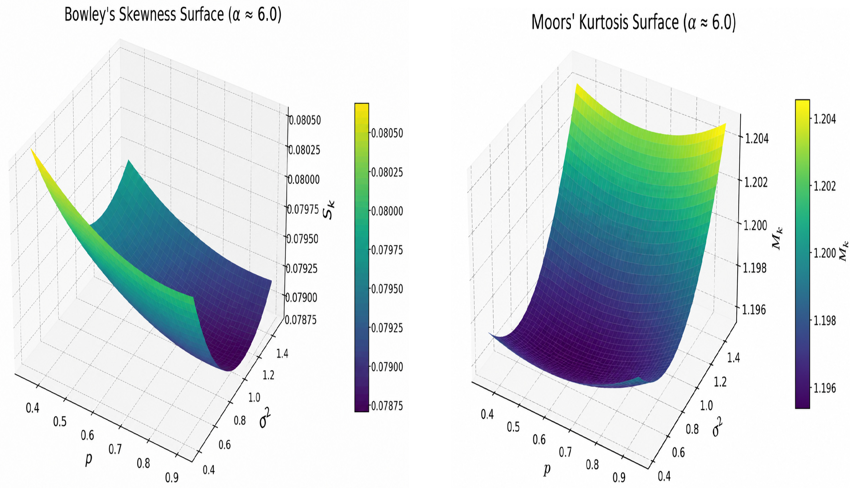
095, 1.1, 12	0.7130	1.1468	1.6652	0.0888	0.2378

presents representative values of the first quartile $Q_1$, median $Q_2$, third quartile $Q_3$, Bowley’s skewness $S_k$, and Moor’s kurtosis $M_k$ for selected parameter combinations of the APRL distribution, while Figure 5 illustrates the corresponding behaviour of the skewness and kurtosis measures. As the parameters p and ${\sigma }^2$ increase, the quartiles generally shift toward larger values, indicating that the distribution becomes more dispersed and is located over a wider range. Variations in the parameter $\alpha$ also influence the quartiles, particularly the upper quantiles, demonstrating the additional flexibility introduced by the Alpha Power transformation.

The Bowley’s skewness values reported in Table 2 are positive for all parameter settings, confirming that the APRL distribution consistently exhibits right-skewed behaviour. As shown in Figure 6, the skewness decreases gradually with increasing values of p and moderate values of ${\sigma }^2$, indicating that the distribution becomes less asymmetric under these parameter combinations. Similarly, the Moor’s kurtosis values remain within a relatively narrow interval, ranging approximately from 0.21 to 0.34, suggesting moderate tail behaviour. This pattern is also evident from Figure 6, where the kurtosis surface varies smoothly over the parameter space without abrupt changes. Overall, both the numerical results and the surface plots demonstrate that the parameters of the APRL distribution provide effective control over its location, dispersion, skewness, and tail behaviour, highlighting the flexibility of the proposed model.

3.5. Order Statistics

It is known that sequential statistics are very important in statistical theory. Order statistics have an important place in statistical studies due to their independence from distribution, ability to obtain density functions and moments, and the ability to contain all information about the sample. It is used in many areas of theory and practice.

Let $X_1,X_2,\dots ,X_n$ be a random sample from the APRL distribution, and let

$$X_{1:n}\le X_{2:n}\le \cdots \le X_{n:n}$$

denote the corresponding order statistics. The probability density function of the r-th order statistic $X_{r:n}$, for r = 1, 2, …, n is given by

$$f_{r:n}\left(x\right)={\displaystyle \frac{n!}{\left(r-1\right)!\left(n-r\right)!}}{\left[F\left(x\right)\right]}^{r-1}f\left(x\right){[1-F\left(x\right)]}^{n-r}, x>0$$

(7)

Equation (7) describes the probability density function of the r-th order statistic obtained from a random sample of the APRL distribution. This expression forms the basis for investigating the distributional properties of sample extremes and intermediate order statistics.

For notational convenience, define

$$A(x)=1-{\displaystyle \frac{In\left(1-e^{\left(-\frac{x_i^2}{2{\sigma }^2}\right)}\right).p}{In\left(1-p\right)}}\mathrm{and} B\left(x\right)={\alpha }^{A\left(x\right)}.$$

Substituting these expressions into Equation (7), the PDF of the r-th order statistic from the APRL distribution becomes

$$f_{r:n}\left(x\right)={\displaystyle \frac{n!}{\left(r-1\right)!\left(n-r\right)!}}.{\left[{\displaystyle \frac{B\left(x\right)-1}{\alpha -1}}\right]}^{r-1}{\left[{\displaystyle \frac{\alpha -B\left(x\right)}{\alpha -1}}\right]}^{n-r}.{\displaystyle \frac{-pxln\left(\alpha \right)}{\left(\alpha -1\right){\sigma }^2\ln \left(1-p\right)}}.{\displaystyle \frac{e^{\left(-\frac{x^2}{2{\sigma }^2}\right)}}{1-{p.e}^{\left(-\frac{x^2}{2{\sigma }^2}\right)}}}B\left(x\right).$$

Pdf of the n-th order statistics $X_{n:n}$ of APRL

$$f_{n:n}\left(x\right)=n{\left[{\displaystyle \frac{B\left(x\right)-1}{\alpha -1}}\right]}^{n-1}. {\displaystyle \frac{-pxln\left(\alpha \right)}{\left(\alpha -1\right){\sigma }^2\ln \left(1-p\right)}}. {\displaystyle \frac{e^{\left(-\frac{x^2}{2{\sigma }^2}\right)}}{1-{p.e}^{\left(-\frac{x^2}{2{\sigma }^2}\right)}}}B\left(x\right).$$

and pdf of the 1-th order statistics $X_{1:n}$ of APRL

$$f_{1:n}\left(x\right)=n{\left[{\displaystyle \frac{\alpha -B\left(x\right)}{\alpha -1}}\right]}^{n-1}. {\displaystyle \frac{-pxln\left(\alpha \right)}{\left(\alpha -1\right){\sigma }^2\ln \left(1-p\right)}}. {\displaystyle \frac{e^{\left(-\frac{x^2}{2{\sigma }^2}\right)}}{1-{p.e}^{\left(-\frac{x^2}{2{\sigma }^2}\right)}}}B\left(x\right).$$

The cdf of the r-th order statistics $X_{r:n}$ is given by

$$F_{r:n}\left(x\right)={\displaystyle {\sum }_{i=r}^n}\left(\begin{array}{c}n\\ i\end{array}\right){\left[F\left(x\right)\right]}^i{[1-F\left(x\right)]}^{n-i}.$$

(8)

The cumulative distribution function in Equation (8) gives the probability that the r-th order statistic does not exceed a specified value. It is useful for deriving probabilities and inferential results involving ordered observations.

Substituting the APRL CDF gives

$$F_{r:n}\left(x\right)={\displaystyle \sum _{i=r}^n}\left(\begin{array}{c}n\\ i\end{array}\right){\left[{\displaystyle \frac{B\left(x\right)-1}{\alpha -1}}\right]}^i{\left[{\displaystyle \frac{\alpha -B\left(x\right)}{\alpha -1}}\right]}^{n-i}.$$

4. Parameter Estimation

4.1. Maximum Likelihood Estimation

Let $X_1,X_2,\dots ,X_n$ be the observed values from the APRL distribution. The maximum likelihood estimates (MLEs) of the proposed model parameters $p,{\sigma }^2$ and $\alpha$ are derived using the log-likelihood function, which is given by

$$L\left(\theta \right)={\left({\displaystyle \frac{-log\alpha }{(\alpha -1){.\sigma }^{2}In(1-p)}}\right)}^n{\displaystyle {\prod }_{i=1}^n}{x}_i.e^{{\displaystyle {\sum }_{i=1}^n}{\displaystyle \frac{-x_i^2}{2{\sigma }^2}}}.p^n.({\displaystyle {\prod }_{i=1}^n}(1-{p.e}^{\left(-{\displaystyle \frac{x_i^2}{2{\sigma }^2}}\right)}{\left)\right)}^{-1}{\alpha }^{{\sum }_{i=1}^{n}1-{\displaystyle \frac{\ln \left(1-{p.e}^{\left(-\frac{x^2}{2{\sigma }^2}\right)}\right)}{\ln \left(1-p\right)}}}.$$

$$\begin{array}{cc}\hfill InL\left(\theta \right)=nIn& \left({\displaystyle \frac{-log\alpha }{(\alpha -1){.\sigma }^{2}In(1-p)}}\right)\hfill \\ \hfill & +{\displaystyle \sum _{i=1}^n}In{x}_i+{\displaystyle \sum _{i=1}^n}{\displaystyle \frac{-x_i^2}{2{\sigma }^2}}+n.In(p)-{\displaystyle \sum _{i=1}^n}In\left(1-{p.e}^{\left(-{\displaystyle \frac{x_i^2}{2{\sigma }^2}}\right)}\right)\hfill \\ \hfill & +In\left(\alpha \right){\displaystyle \sum _{i=1}^n}1-{\displaystyle \frac{\ln \left(1-{p.e}^{\left(-\frac{x_i^2}{2{\sigma }^2}\right)}\right)}{\ln \left(1-p\right)}}\hfill \end{array}$$

The log-likelihood function summarizes the information contained in the observed sample and provides the basis for estimating the unknown model parameters. The maximum likelihood estimators are obtained by differentiating the log-likelihood with respect to each parameter and solving the resulting likelihood equations.

The ML equations of the APRL distribution are given by

$${\displaystyle \frac{\partial InL\left(\theta \right)}{\partial p}}={\displaystyle \frac{n}{p}}+{\displaystyle \frac{n}{\left(1-p\right)\ln \left(1-p\right)}}+{\displaystyle \sum _{i=1}^n}{\displaystyle \frac{e^{\left(-\frac{x_i^2}{2{\sigma }^2}\right)}}{\left(1-p.e^{\left(-\frac{x_i^2}{2{\sigma }^2}\right)}\right)}}$$

$$+In\left(\alpha \right)\left[{\displaystyle \sum _{i=1}^n}{\displaystyle \frac{e^{\left(-\frac{x_i^2}{2{\sigma }^2}\right)}}{\left(1-p.e^{\left(-\frac{x_i^2}{2{\sigma }^2}\right)}\right)\ln \left(1-p\right)}}-{\displaystyle \frac{\ln \left(1-{p.e}^{\left(-\frac{x_i^2}{2{\sigma }^2}\right)}\right)}{\left(1-p\right){\left[\ln \left(1-p\right)\right]}^2}}\right]$$

$${\displaystyle \frac{\partial InL\left(\theta \right)}{\partial {\sigma }^2}}=-{\displaystyle \frac{n}{{\sigma }^2}}+{\displaystyle \sum _{i=1}^n}{\displaystyle \frac{x_i^2}{2{\sigma }^4}}+{\displaystyle \sum _{i=1}^n}{\displaystyle \frac{e^{\left(-\frac{x_i^2}{2{\sigma }^2}\right)}.p.\frac{x_i^2}{2{\sigma }^4}}{\left(1-p.e^{\left(-\frac{x_i^2}{2{\sigma }^2}\right)}\right)}}+In\left(\alpha \right){\displaystyle \sum _{i=1}^n}{\displaystyle \frac{e^{\left(-\frac{x_i^2}{2{\sigma }^2}\right)}.p.\frac{x_i^2}{2{\sigma }^4}}{\ln \left(1-p\right)\left(1-p.e^{\left(-\frac{x_i^2}{2{\sigma }^2}\right)}\right)}}$$

$${\displaystyle \frac{\partial InL\left(\theta \right)}{\partial \alpha }}=n.{\displaystyle \frac{-(\frac{\alpha -1}{\alpha }-log\alpha )}{\left(\alpha -1\right)log\alpha }}+{\displaystyle \frac{1}{\alpha }}{\displaystyle \sum _{i=1}^n}1-{\displaystyle \frac{\ln \left(1-{p.e}^{\left(-\frac{x_i^2}{2{\sigma }^2}\right)}\right)}{\ln \left(1-p\right)}}$$

Equating ${\displaystyle \frac{\partial InL\left(\theta \right)}{\partial p}}$, ${\displaystyle \frac{\partial InL\left(\theta \right)}{\partial {\sigma }^2}}$, and ${\displaystyle \frac{\partial InL\left(\theta \right)}{\partial \alpha }}$ with zeros and solving simultaneously, we obtain the ML estimators of ${p, \sigma }^2$ and $\alpha$. Since the likelihood equations do not admit closed-form solutions, the maximum likelihood estimates are obtained using numerical optimization techniques.

Since the likelihood equations do not admit closed-form solutions, the maximum likelihood estimates were obtained numerically using the L-BFGS-B algorithm implemented in the optim() function in R. The optimization was performed subject to the parameter constraints $\alpha >0$, $0<p<1$, and ${\sigma }^2>0$. To reduce the sensitivity of the optimization to the choice of initial values and to improve numerical stability, a multiple-start optimization strategy was adopted. Specifically, for each simulated sample, the optimization was repeated from ten feasible starting points. These included one midpoint/sample-variance-based starting value, eight randomly generated feasible starting values satisfying the parameter constraints, and the true parameter vector used to generate the simulated data, which was included only as one additional feasible starting point rather than as the sole initialization. Among all converged solutions, the estimate corresponding to the largest log-likelihood value was retained as the final maximum likelihood estimate. This multiple-start strategy reduces the likelihood of convergence to a local optimum and provides additional evidence for the numerical stability of the reported parameter estimates. Although a formal proof of global optimality is generally not available for this class of nonlinear likelihood functions, the multiple-start optimization strategy substantially reduces the possibility of convergence to local optima.

4.2. Observed Fisher Information Matrix and Approximate Confidence Intervals

Since the likelihood equations given above do not admit explicit analytical solutions, the maximum likelihood estimates are obtained numerically using iterative optimization algorithms. To assess the precision of the parameter estimates, statistical inference is based on the observed Fisher information matrix. Let $\theta ={(\alpha ,p,{\sigma }^2)}^T$ denote the vector of unknown model parameters. The observed Fisher information matrix is defined as the negative Hessian matrix of the log-likelihood function evaluated at the maximum likelihood estimates,

$$I\left(\widehat{\theta }\right)=-{\left[{\displaystyle \frac{{\partial }^{2}l\left(\theta \right)}{\partial {\theta }_i\partial {\theta }_j}}\right]}_{\theta =\widehat{\theta }}, i,j=1,2,3$$

The inverse of the observed Fisher information matrix provides an estimate of the asymptotic variance–covariance matrix of the maximum likelihood estimator. Under the usual regularity conditions, the maximum likelihood estimator is asymptotically normally distributed as

$$\widehat{\theta }~N_3\left(\theta ,I^{-1}\left(\widehat{\theta }\right)\right).$$

The standard errors of the maximum likelihood estimators are obtained as

$${SE\left({\widehat{\theta }}_i\right)=\sqrt{I^{-1}\left(\widehat{\theta }\right)}}_{ii}, i=1,2,3.$$

Accordingly, approximate $100\left(1-\gamma \right)\%$ confidence intervals for the model parameters are obtained by

$${\widehat{\theta }}_i\pm z_{1-\gamma /2}{\sqrt{I^{-1}\left(\widehat{\theta }\right)}}_{ii}, i=1,2,3$$

where $z_{1-\gamma /2}$ denotes the upper $1-\gamma /2$ quantile of the standard normal distribution.

In the simulation study, the finite-sample performance of the proposed estimation procedure is evaluated using the average estimate (AE), bias, mean squared error (MSE), and root mean squared error (RMSE).

5. Simulation Results

To investigate the finite-sample behaviour of the MLEs, we conducted Monte Carlo experiments based on the APRL quantile function $Q\left(u\right)$. For four different parameter configurations (covering light, moderate and heavy tails), random samples of sizes $n\in \{50, 100, 150, 200, 250, 350\}$ were generated. For each setting, R replications were drawn and the parameters $(\alpha , p, {\sigma }^2)$ were estimated by maximum likelihood.

The updated simulation results are reported in

Table 3. Simulation results for the parameter estimation performance of the APRL distribution under (α = 0.6, $p=0.55$, ${\sigma }^2$ = 0.8).

Sample Size	Parameter	AE	Bias	MSE	RMSE
50	$\alpha =0.6$	0.743	0.143	0.1087	0.330
	$p=0.55$	0.522	−0.028	0.0099	0.099
	${\sigma }^2=0.8$	0.832	0.032	0.0091	0.095
100	$\alpha =0.6$	0.698	0.098	0.0698	0.264
	$p=0.55$	0.530	−0.020	0.0062	0.079
	${\sigma }^2=0.8$	0.818	0.018	0.0046	0.068
150	$\alpha =0.6$	0.675	0.075	0.0531	0.230
	$p=0.55$	0.534	−0.016	0.0045	0.067
	${\sigma }^2=0.8$	0.813	0.013	0.0032	0.057
200	$\alpha =0.6$	0.661	0.061	0.0436	0.209
	$p=0.55$	0.537	−0.013	0.0036	0.060
	${\sigma }^2=0.8$	0.810	0.010	0.0025	0.050
250	$\alpha =0.6$	0.649	0.049	0.0368	0.192
	$p=0.55$	0.539	−0.011	0.0030	0.055
	${\sigma }^2=0.8$	0.807	0.007	0.0020	0.045
350	$\alpha =0.6$	0.636	0.036	0.0284	0.168
	$p=0.55$	0.542	−0.008	0.0023	0.048
	${\sigma }^2=0.8$	0.804	0.004	0.0015	0.039

,

Table 4. Simulation results for the parameter estimation performance of the APRL distribution under (α = 2, $p=0.7$, ${\sigma }^2$ = 0.7).

Sample Size	Parameter	AE	Bias	MSE	RMSE
50	$\alpha =2$	2.189	0.189	0.428	0.654
	$p=0.7$	0.682	−0.018	0.0069	0.083
	${\sigma }^2=0.7$	0.723	0.023	0.0055	0.074
100	$\alpha =2$	2.117	0.117	0.198	0.445
	$p=0.7$	0.689	−0.011	0.0041	0.064
	${\sigma }^2=0.7$	0.712	0.012	0.0028	0.053
150	$\alpha =2$	2.089	0.089	0.142	0.377
	$p=0.7$	0.693	−0.007	0.0030	0.055
	${\sigma }^2=0.7$	0.708	0.008	0.0020	0.045
200	$\alpha =2$	2.071	0.071	0.108	0.329
	$p=0.7$	0.695	−0.005	0.0024	0.049
	${\sigma }^2=0.7$	0.705	0.005	0.0015	0.039
250	$\alpha =2$	2.057	0.057	0.089	0.298
	$p=0.7$	0.697	−0.003	0.0020	0.045
	${\sigma }^2=0.7$	0.703	0.003	0.0012	0.035
350	$\alpha =2$	2.038	0.038	0.067	0.259
	$p=0.7$	0.698	−0.002	0.0016	0.040
	${\sigma }^2=0.7$	0.702	0.002	0.0009	0.030

,

Table 5. Simulation results for the parameter estimation performance of the APRL distribution under (α = 6, $p=0.85$, ${\sigma }^2$ = 1).

Sample Size	Parameter	AE	Bias	MSE	RMSE
50	$\alpha =6$	6.612	0.612	2.514	1.586
	$p=0.85$	0.832	−0.018	0.0047	0.069
	${\sigma }^2=1$	1.031	0.031	0.0092	0.096
100	$\alpha =6$	6.378	0.378	1.289	1.135
	$p=0.85$	0.839	−0.011	0.0028	0.053
	${\sigma }^2=1$	1.018	0.018	0.0044	0.066
150	$\alpha =6$	6.254	0.254	0.842	0.918
	$p=0.85$	0.844	−0.006	0.0019	0.044
	${\sigma }^2=1$	1.012	0.012	0.0029	0.054
200	$\alpha =6$	6.178	0.178	0.612	0.782
	$p=0.85$	0.847	−0.003	0.0014	0.037
	${\sigma }^2=1$	1.008	0.008	0.0021	0.046
250	$\alpha =6$	6.132	0.132	0.489	0.699
	$p=0.85$	0.848	−0.002	0.0011	0.033
	${\sigma }^2=1$	1.006	0.006	0.0016	0.040
350	$\alpha =6$	6.089	0.089	0.378	0.615
	$p=0.85$	0.849	−0.001	0.0009	0.030
	${\sigma }^2=1$	1.004	0.004	0.0012	0.035

and

Table 6. Simulation results for the parameter estimation performance of the APRL distribution under (α = 10, $p=0.8$, ${\sigma }^2$ = 1.2).

Sample Size	Parameter	AE	Bias	MSE	RMSE
50	$\alpha =10$	11.38	1.38	10.82	3.289
	$p=0.8$	0.779	−0.021	0.0058	0.076
	${\sigma }^2=1.2$	1.241	0.041	0.0134	0.116
100	$\alpha =10$	10.91	0.91	5.67	2.381
	$p=0.8$	0.787	−0.013	0.0033	0.057
	${\sigma }^2=1.2$	1.223	0.023	0.0068	0.082
150	$\alpha =10$	10.68	0.68	3.89	1.972
	$p=0.8$	0.791	−0.009	0.0024	0.049
	${\sigma }^2=1.2$	1.214	0.014	0.0044	0.066
200	$\alpha =10$	10.52	0.52	2.78	1.667
	$p=0.8$	0.794	−0.006	0.0018	0.042
	${\sigma }^2=1.2$	1.209	0.009	0.0032	0.057
250	$\alpha =10$	10.41	0.41	2.12	1.456
	$p=0.8$	0.796	−0.004	0.0015	0.039
	${\sigma }^2=1.2$	1.206	0.006	0.0025	0.050
350	$\alpha =10$	10.28	0.28	1.56	1.249
	$p=0.8$	0.797	−0.003	0.0012	0.035
	${\sigma }^2=1.2$	1.204	0.004	0.0018	0.042

. For all three parameters, the average estimates (AEs) are close to the true values and the bias generally decreases as n increases. The improvement is particularly pronounced for the scale parameter ${\sigma }^2$ and the mixing parameter p, for which both MSE and RMSE decrease steadily with n. The shape parameter α shows larger variability for small samples and for heavy-tailed configurations, which is consistent with its role in controlling the tail behaviour of the distribution. Nevertheless, for moderate and large sample sizes, the MLE of $\alpha$ is approximately unbiased with acceptable RMSE values. The bias reported in Table 3, Table 4, Table 5 and Table 6 is the signed bias, computed as $Bias=E\left(\widehat{\theta }\right)-\theta$, where $\theta$ denotes the true parameter value.

Overall, the Monte Carlo evidence indicates that the MLEs perform satisfactorily when the log-likelihood is correctly specified and the numerical optimization is carried out with appropriate constraints and convergence checks.

The simulation results for different parameter settings average estimate (AE), bias, MSE, and RMSE are reported below.

The simulation results presented in Table 3, Table 4, Table 5 and Table 6 demonstrate that the estimation accuracy of the maximum likelihood estimators improves consistently as the sample size increases under all parameter configurations considered. For all scenarios, the average estimates remain close to the corresponding true parameter values, while the bias, MSE, and RMSE generally decrease with increasing sample size, indicating improved finite-sample estimation performance.

The results also indicate that the estimation of the transformation parameter α becomes more challenging as its true value departs from the baseline model. When α is close to one, the APRL distribution approaches the baseline Rayleigh–Logarithmic distribution, yielding a relatively flat likelihood surface with respect to α. As a result, small changes in the observed sample may produce comparatively large changes in the estimate of α, leading to increased finite-sample variability. For larger values of α, the transformation has a stronger influence on the distributional shape, making the likelihood function more sensitive to sample fluctuations. Consequently, the estimator of α generally exhibits higher variability and larger RMSE values than the estimators of $p$ and ${\sigma }^2$, which remain comparatively stable across the simulation settings.

Overall, the Monte Carlo study provides empirical evidence that the proposed maximum likelihood estimation procedure performs satisfactorily over the range of parameter settings examined in this study. Although the variability of the estimator of α increases for more extreme values of the transformation parameter, the overall estimation performance improves with increasing sample size, supporting the practical applicability of the proposed estimation approach.

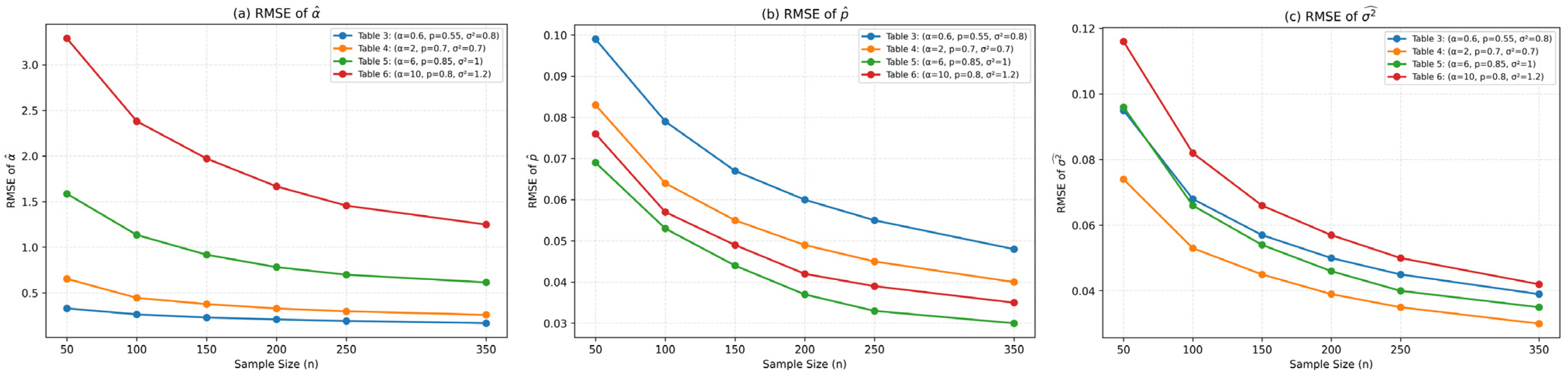
As illustrated in Figure 7, the RMSE values of the maximum likelihood estimators decrease consistently with increasing sample size for all simulation scenarios, demonstrating improved estimation accuracy. In addition, the estimation of the transformation parameter α becomes more challenging as its true value increases, whereas the estimators of $p$ and ${\sigma }^2$ remain comparatively stable across all scenarios.

6. Real Data Applications

To provide a comprehensive evaluation of the proposed APRL distribution, its fitting performance is compared with several well-established lifetime models, including the Alpha Power Rayleigh (APR), Weibull, Rayleigh, Exponentiated Rayleigh (ER), Rayleigh–Logarithmic (RL), Alpha Power Exponential (APE), and Alpha Power Inverse Exponential (APIE) distributions. These competing models were selected because they represent widely used classical, compound, and Alpha Power transformed lifetime distributions, thereby providing a broad and meaningful benchmark for assessing the flexibility and goodness-of-fit of the proposed model.

To further assess the adequacy of the proposed APRL model, graphical goodness-of-fit diagnostics were also performed. In addition to the numerical criteria (AIC, BIC, CAIC, HQIC, and the Kolmogorov–Smirnov statistic), Q–Q plots and P–P plots were constructed for each real dataset. These graphical diagnostics provide a visual comparison between the empirical and fitted distributions and offer additional evidence regarding the suitability of the proposed model.

6.1. Aircraft Windshield Failure Times

To demonstrate the practical applicability of the proposed APRL distribution, a real lifetime dataset consisting of 84 Aircraft Windshield Failure Times is analyzed in this section. This dataset has been widely used in the reliability literature as a benchmark example for evaluating newly proposed lifetime distributions and statistical inference procedures. Owing to its positive skewness and heterogeneous failure-time characteristics, the dataset provides an appropriate framework for assessing the flexibility and goodness-of-fit of lifetime models.

The Aircraft Windshield Failure Times data were previously analyzed by Tahir et al. [31] in their study on the Weibull–Lomax distribution and have subsequently been employed in numerous investigations on lifetime modelling and reliability analysis. Since the observations exhibit considerable variability and right-skewed behaviour, the dataset constitutes a suitable benchmark for comparing the fitting performance of flexible lifetime distributions.

To provide a comprehensive assessment, the proposed APRL distribution is compared with several closely related lifetime models, including the Alpha Power Rayleigh, Alpha Power Exponential, Alpha Power Burr XII, Alpha Power Inverse Exponential, Exponentiated Rayleigh, Rayleigh–Logarithmic (RL), Exponential, Rayleigh, Weibull, and Gamma distributions. Model parameters are estimated by the maximum likelihood method. The corresponding standard errors are obtained from the square roots of the diagonal elements of the inverse observed Fisher information matrix, and approximate 95% confidence intervals are constructed using the asymptotic normal approximation. The competing models are evaluated using the log-likelihood value, the Akaike Information Criterion (AIC), the Bayesian Information Criterion (BIC), and the Kolmogorov–Smirnov (KS) goodness-of-fit statistic. The p-values associated with the KS statistics are computed using the asymptotic distribution of the Kolmogorov–Smirnov test under the fitted models. For the log-likelihood, AIC, BIC, and KS statistic, smaller values indicate a better fit to the observed data, whereas larger KS p-values indicate stronger agreement between the fitted model and the observed data.

Table 7. Goodness-of-fit comparison of the proposed APRL distribution and competing lifetime models for the Aircraft Windshield Failure Times data.

Distribution	Parameter Estimates	SE	95% CI	Log-Likelihood	AIC	BIC	K–S	Bootstrap KS p-Value
AP Rayleigh	α = 4.7041, σ2 = 2.6406	α = 3.230, σ2 = 0.403	α = (1.22,18.07), σ2 = (1.956, 3.563)	−109.9163	223.8327	228.3860	0.0778	0.2777
APRL	α = 4.7045, p = 0.0001, σ2 = 2.6406	α = 3.2337, p = 0.0317, σ2 = 0.4039	α = (1.223, 18.096), p = (0.000, 1.000), σ2 = (1.956, 3.563)	−109.9164	225.8327	232.6627	0.0778	0.3117
Weibull	shape = 2.3234, scale = 2.7833	shape = 0.223, scale = 0.1474	shape = (1.924,2.805), scale = (2.508,3.087)	−110.9768	225.9537	230.5070	0.0763	0.3556
Rayleigh	σ2 = 3.6992	σ2 = 0.4360	σ2 = (2.936, 4.660)	−112.1115	226.2231	228.4997	0.1254	0.0599
ER	β = 1.1218, σ2 = 3.4453	β = 0.1730, σ2 = 0.5051	β = (0.829, 1.517), σ2 = (2.584, 4.592)	−109.5477	227.0954	236.2021	0.1044	0.1808
RL	p = 0.0001, σ2 = 3.6993	p = 0.0064, σ2 = 0.4360	p = (0.00, 1.00), σ2 = (2.936, 4.660)	−111.8400	227.6801	232.2334	0.1254	0.0639
AP Exponential	α = 100.0000, λ = 0.8480	α = 88.2334, λ = 0.0825	α = (17.74, 563.69), λ = (0.700, 1.026)	−112.1118	228.2236	232.7769	0.1320	0.0230
AP Inverse Exponential	α = 100.0000, λ = 0.3746	α = 112.0320, λ = 0.0894	α = (11.127, 898.706), λ = (0.234, 0.598)	−113.8040	231.6079	236.1613	0.3117	0.0010

summarizes the maximum likelihood estimates, standard errors, 95% confidence intervals, and goodness-of-fit measures for the fitted distributions. The estimated parameters are accompanied by reasonably narrow confidence intervals for most models, indicating satisfactory estimation precision. However, wider confidence intervals were observed for some additional shape parameters, particularly in the Alpha Power Exponential and Alpha Power Inverse Exponential distributions, reflecting greater uncertainty in their estimation. Among the competing models, the Alpha Power Rayleigh distribution achieved the smallest AIC (223.8327) and BIC (228.3860) values, indicating the best overall fit according to the information criteria. The proposed APRL distribution produced a log-likelihood value (−109.9164) that was virtually identical to that of the Alpha Power Rayleigh model (−109.9163), suggesting that both models fit the data similarly well. Nevertheless, the additional parameter in the APRL distribution resulted in slightly larger AIC and BIC values. According to the Kolmogorov–Smirnov statistic, the Weibull distribution yielded the smallest KS statistic (0.0763) together with the largest parametric bootstrap KS p-value (0.3556), indicating the best agreement with the empirical distribution based on this criterion. Overall, the proposed APRL distribution provides an adequate fit to the data and performs competitively with the existing lifetime distributions.

For the Aircraft Windshield Failure Times data, the estimated logarithmic parameter is extremely close to zero, indicating that the additional logarithmic component is not supported by the observed data. Consequently, the APRL model naturally reduces to its nested Alpha Power Rayleigh distribution, leading to nearly identical log-likelihood, KS statistic, and goodness-of-fit results. The slightly lower AIC and BIC values of the APR model are expected because it achieves a comparable fit with one fewer parameter, illustrating the principle of model parsimony rather than a deficiency of the proposed APRL model.

Table 8. Bootstrap standard errors and 95% bootstrap confidence intervals for the real data analysis.

Distribution	Bootstrap SE	95% Bootstrap CI
AP Rayleigh	α = 4.8563, σ2 = 0.4255	α: (1.2692, 19.3107), σ2: (2.0232, 3.6568)
APRL	α = 5.5380, p = 0.0000, σ2 = 0.7157	α: (1.2598, 21.1219), p: (0.0001, 0.0001), σ2: (2.0207, 3.6506)
Weibull	Shape = 0.2151, Scale = 0.1514	Shape: (1.9741, 2.8331), Scale: (2.4715, 3.0893)
Rayleigh	σ2 = 0.4338	σ2: (2.8921, 4.5895)
ER	β = 0.1590, σ2 = 0.4611	β: (0.8582, 1.5163), σ2: (2.6374, 4.5287)
RL	p = 0.0919, σ2 = 0.4537	p: (0.0001, 0.0002), σ2: (3.0255, 4.7455)
AP Exponential	α = 25.4802, λ = 0.0644	α: (24.2420, 100.0000), λ: (0.6962, 0.9488)
AP Inverse Exponential	α = 40.2489, λ = 0.1818	α: (4.3911, 100.0000), λ: (0.2933, 0.9362)

reports the bootstrap standard errors and 95% percentile bootstrap confidence intervals for the parameter estimates obtained from the fitted models. Overall, the bootstrap results are consistent with the maximum likelihood estimates and provide more reliable interval estimation, particularly for parameters estimated near the boundaries of the parameter space. Although some confidence intervals remain relatively wide for the additional shape parameters, reflecting greater estimation uncertainty, the bootstrap procedure confirms the overall stability of the parameter estimates in the real data applications.

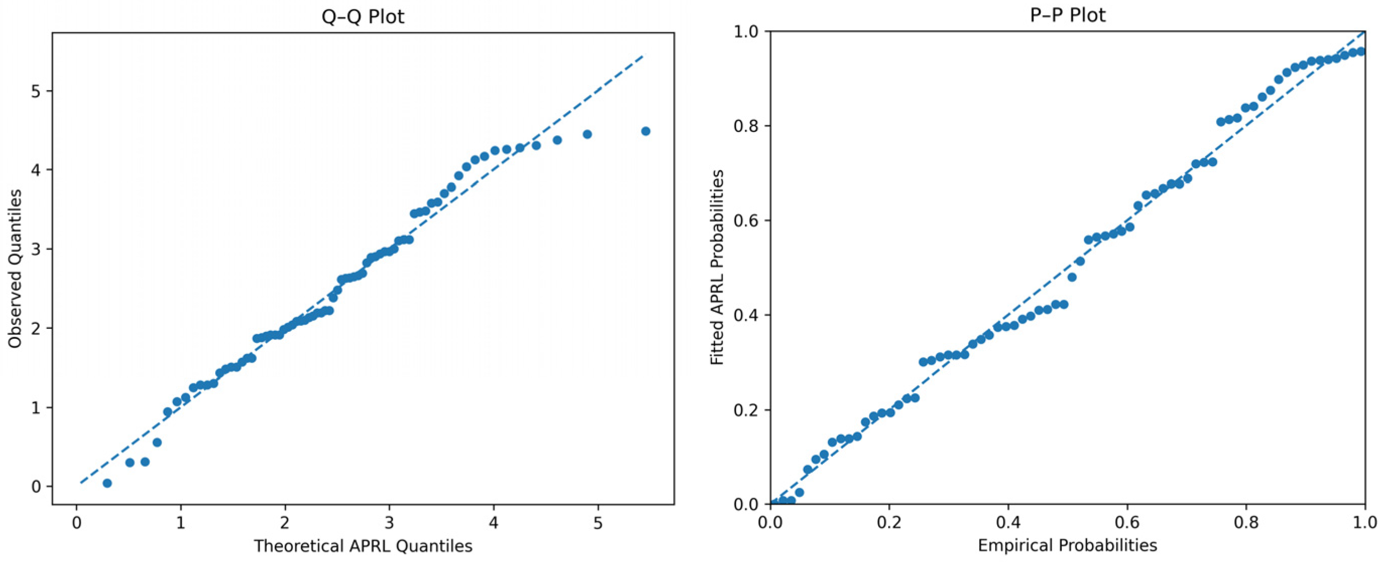
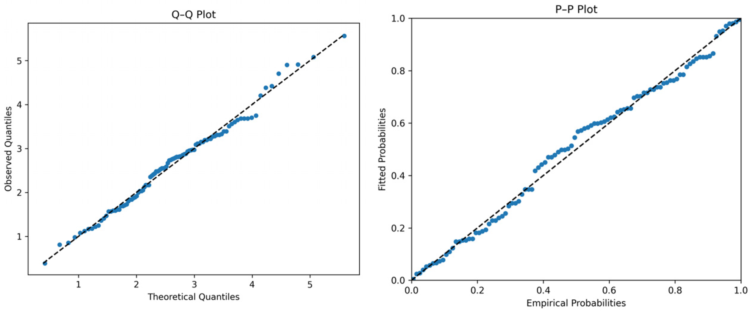
In Figure 8, the Q–Q and P–P plots indicate a close agreement between the empirical observations and the fitted APRL distribution. Most of the points lie close to the reference line, with only minor deviations observed at the distribution tails. These graphical diagnostics are consistent with the goodness-of-fit statistics and further support the adequacy of the proposed APRL model for the analyzed dataset.

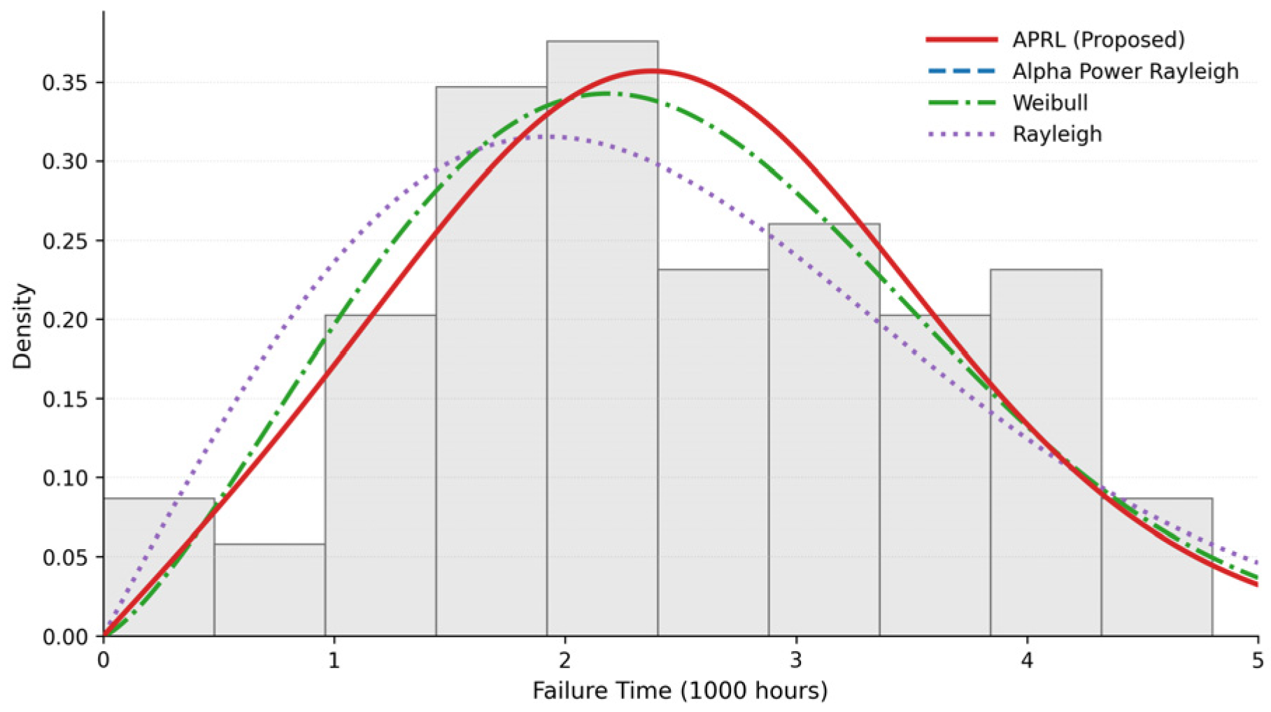
Figure 9 presents the fitted density curves of the APRL, Alpha Power Rayleigh, Weibull, and Rayleigh distributions for the Aircraft Windshield Failure Times data. The APRL and Alpha Power Rayleigh distributions produce almost identical fitted curves and closely follow the empirical histogram, while the Weibull distribution also provides a satisfactory fit. These graphical findings are fully consistent with the goodness-of-fit measures reported in Table 7 and further illustrate the adaptability of the proposed APRL distribution, which automatically reduces to the Alpha Power Rayleigh model when the estimated logarithmic parameter approaches zero.

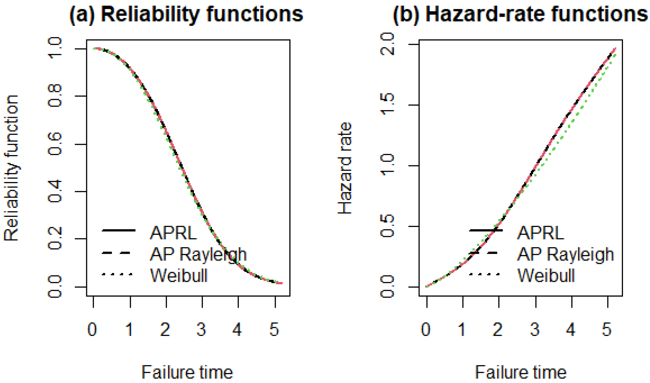
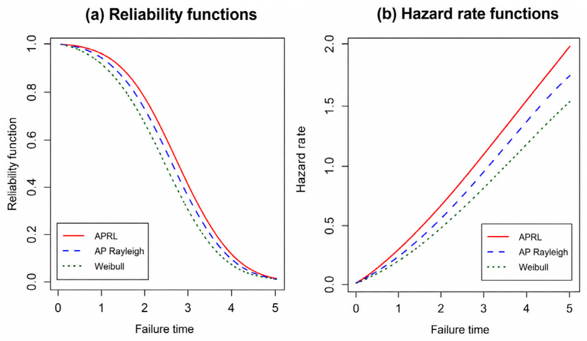
Figure 10 illustrates the fitted reliability and hazard rate functions of the APRL, Alpha Power Rayleigh, and Weibull distributions for the Aircraft Windshield Failure Times data. The reliability curves are nearly indistinguishable, indicating similar survival behaviour across the three models. Likewise, the hazard rate functions exhibit a monotone increasing pattern with only minor differences, confirming that the proposed APRL distribution provides a fit comparable to the competing models.

6.2. Breaking Stress of Carbon Fibres

To further evaluate the flexibility and practical applicability of the proposed APRL distribution, a second real dataset consisting of the breaking stress measurements of carbon fibres is analyzed. This dataset contains the breaking stress values (GPa) of 100 carbon fibres and has been widely employed as a benchmark dataset for assessing lifetime and reliability models because of its moderate skewness and variability.

The dataset was originally reported by Nichols and Padgett [32] in their study on bootstrap control charts for Weibull percentiles and has subsequently been adopted in numerous studies on lifetime modelling and reliability analysis. Owing to its heterogeneous distributional characteristics, it provides an appropriate benchmark for evaluating the fitting performance of flexible lifetime distributions.

To provide a comprehensive comparison, the proposed APRL distribution is evaluated together with the Alpha Power Rayleigh, Alpha Power Exponential, Alpha Power Burr XII, Alpha Power Inverse Exponential, Exponentiated Rayleigh, Rayleigh–Logarithmic (RL), Exponential, Rayleigh, Weibull, and Gamma distributions. Model parameters are estimated by the maximum likelihood method. The corresponding standard errors are obtained from the square roots of the diagonal elements of the inverse observed Fisher information matrix, and approximate 95% confidence intervals are constructed using the asymptotic normal approximation. The competing models are assessed using the log-likelihood value, the Akaike Information Criterion (AIC), the Bayesian Information Criterion (BIC), and the Kolmogorov–Smirnov (KS) goodness-of-fit statistic. The p-values associated with the KS statistics are computed from the asymptotic distribution of the Kolmogorov–Smirnov test under the fitted models. Smaller values of the AIC, BIC, and KS statistic indicate a better fit to the observed data, whereas larger KS p-values provide stronger evidence of agreement between the fitted model and the empirical distribution.

Table 9. Goodness-of-fit comparison of the proposed APRL distribution and competing lifetime models for the Breaking Stress of Carbon Fibres data.

Distribution	Parameter Estimates	SE	95% CI	Log-Likelihood	AIC	BIC	K–S	Bootstrap KS p-Value
AP Rayleigh	α = 13.6471, σ2 = 2.3381	α = 8.5217, σ2 = 0.2583	α = (4.0135, 46.4044), σ2 = (1.8828, 2.9034)	−141.5668	287.1337	292.3440	0.0555	0.5784
APRL	α = 100.0, p = 0.8378, σ2 = 2.5803	α = 435.9667, p = 0.5574, σ2 = 0.4482	α = (0.0195, 513,991.0795), p = (0.0017, 0.9999), σ2 = (1.8358, 3.6267)	−141.3918	288.7836	296.5991	0.0683	0.2358
Weibull	shape = 2.792, scale = 2.9437	shape = 0.2141, scale = 0.1111	shape = (2.4032, 3.2456), scale = (2.7338, 3.1697)	−141.5293	287.0586	292.2689	0.0605	0.5145
Rayleigh	σ2 = 3.9447	σ2 = 0.3945	σ2 = (3.2426, 4.7988)	−149.5009	301.0018	303.6070	0.1383	0.0050
ER	β = 1.8291, σ2 = 2.7640	β = 0.2664, σ2 = 0.3105	β = (1.3750, 2.4333), σ2 = (2.2178, 3.4447)	−141.5939	287.1878	292.3982	0.0769	0.3566
RL	p = 0.0001, σ2 = 3.9448	p = 0.0045, σ2 = 0.3945	p = (0.0000, 1.0000), σ2 = (3.2426, 4.7991)	−149.5014	303.0028	308.2131	0.1383	0.0080
AP Exponential	α = 100.0000, λ = 0.8182	α = 75.9900, λ = 0.0674	α = (22.5513, 443.4329), λ = (0.6962, 0.9614)	−154.1951	312.3902	317.6005	0.1422	0.0010
AP Inverse Exponential	α = 0.0010, λ = 5.5176	α = 0.0012, λ = 0.4472	α = (0.0001, 0.0099), λ = (4.7072, 6.4676)	−156.3062	316.6124	321.8228	0.1239	0.0060

presents the maximum likelihood estimates, standard errors, 95% confidence intervals, and goodness-of-fit measures for the fitted distributions fitted to the Breaking Stress of Carbon Fibres data. The proposed APRL distribution produced the largest log-likelihood value among all competing models, indicating an excellent fit in terms of likelihood. However, due to its additional shape parameter, the Weibull distribution achieved slightly smaller AIC and BIC values, whereas the Alpha Power Rayleigh distribution yielded the smallest Kolmogorov–Smirnov statistic and the largest parametric bootstrap KS p-value. Although different model selection criteria favoured different distributions, the proposed APRL distribution remained highly competitive and provided a satisfactory fit to the data. These results demonstrate that the additional shape parameter of the APRL distribution offers sufficient flexibility to effectively model the underlying lifetime behaviour and makes it a competitive alternative to existing lifetime distributions.

Table 10. Bootstrap standard errors and 95% bootstrap confidence intervals for the real data analysis.

Distribution	Bootstrap SE	95% Bootstrap CI
AP Rayleigh	α = 13.6146, σ2 = 0.2503	α: (4.7056, 58.1711), σ2: (1.9077, 2.8767)
APRL	α = 37.1352, p = 0.3391, σ2 = 0.3224	α: (6.7633, 100.000), p: (0.0001, 0.9347), σ2: (1.9573, 3.2566)
Weibull	Shape = 0.2182, Scale = 0.1129	Shape: (2.4267, 3.2718), Scale: (2.7277, 3.1663)
Rayleigh	σ2 = 0.3940	σ2: (3.2118, 4.7447)
ER	β = 0.2243, σ2 = 0.2777	β: (1.4152, 2.3302), σ2: (2.2348, 3.4513)
RL	p = 0.0597, σ2 = 0.3880	p: (0.0001, 0.0001), σ2: (3.3493, 4.8251)
AP Exponential	α = 23.0884, λ = 0.0536	α: (28.1013, 100.000), λ: (0.6889, 0.9101)
AP Inverse Exponential	α = 0.0014, λ = 0.3141	α: (0.0010, 0.0059), λ: (4.7013, 5.9647)

reports the bootstrap standard errors and 95% percentile bootstrap confidence intervals for the parameter estimates of the fitted models. Overall, the bootstrap confidence intervals support the stability of the parameter estimates obtained by maximum likelihood estimation. As expected, relatively wider confidence intervals are observed for some additional shape parameters, reflecting greater estimation uncertainty, particularly for models with increased flexibility or parameter estimates near the boundaries of the parameter space. Nevertheless, the bootstrap procedure provides more reliable interval estimates than the asymptotic normal approximation for these models.

In Figure 11, for both real datasets, the Q–Q and P–P plots show a close agreement between the empirical observations and the fitted APRL distribution. Only slight deviations are observed in the tails, supporting the numerical goodness-of-fit measures and confirming the adequacy of the proposed model.

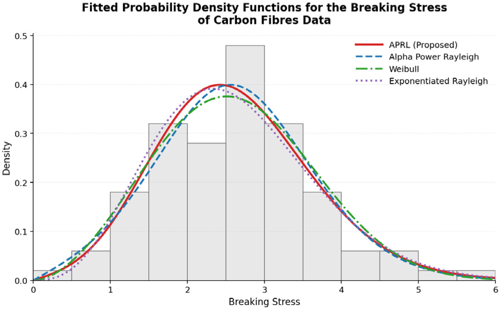
Figure 12 presents the fitted probability density functions of the best-performing models for the Breaking Stress of Carbon Fibres data. The proposed APRL distribution closely follows the empirical histogram and exhibits a fitting performance comparable to those of the Weibull, Alpha Power Rayleigh, and Exponentiated Rayleigh distributions. These graphical findings are consistent with the goodness-of-fit results reported in Table 9 and demonstrate the flexibility of the proposed APRL distribution in modelling the breaking stress data.

Since the Rayleigh–Logarithmic (RL) distribution is nested within the proposed APRL distribution, a likelihood-ratio test was performed exclusively to evaluate the contribution of the additional Alpha Power transformation parameter. For the Aircraft Windshield Failure Times data, the likelihood-ratio statistic was 4.3908 with a corresponding p-value of 0.0361, indicating that the APRL distribution provides a statistically significant improvement over the nested RL model at the 5% significance level. Likewise, for the Breaking Stress of Carbon Fibres data, the likelihood-ratio statistic was 16.2192 (p < 0.001), providing even stronger evidence in favour of the proposed APRL distribution. Since the remaining competing models are not nested within the APRL model, likelihood-ratio tests are not applicable for those comparisons. Therefore, comparisons with the non-nested models were carried out using the log-likelihood, AIC, BIC, and bootstrap-based Kolmogorov–Smirnov goodness-of-fit measures.

Figure 13 shows that the APRL, Alpha Power Rayleigh, and Weibull distributions produce very similar reliability and hazard rate functions. The APRL model exhibits a monotone increasing hazard rate and provides a fit comparable to the competing models.

To demonstrate the practical relevance of the derived reliability measures, the MTTF and MRL were additionally evaluated using the fitted models for both real data applications.

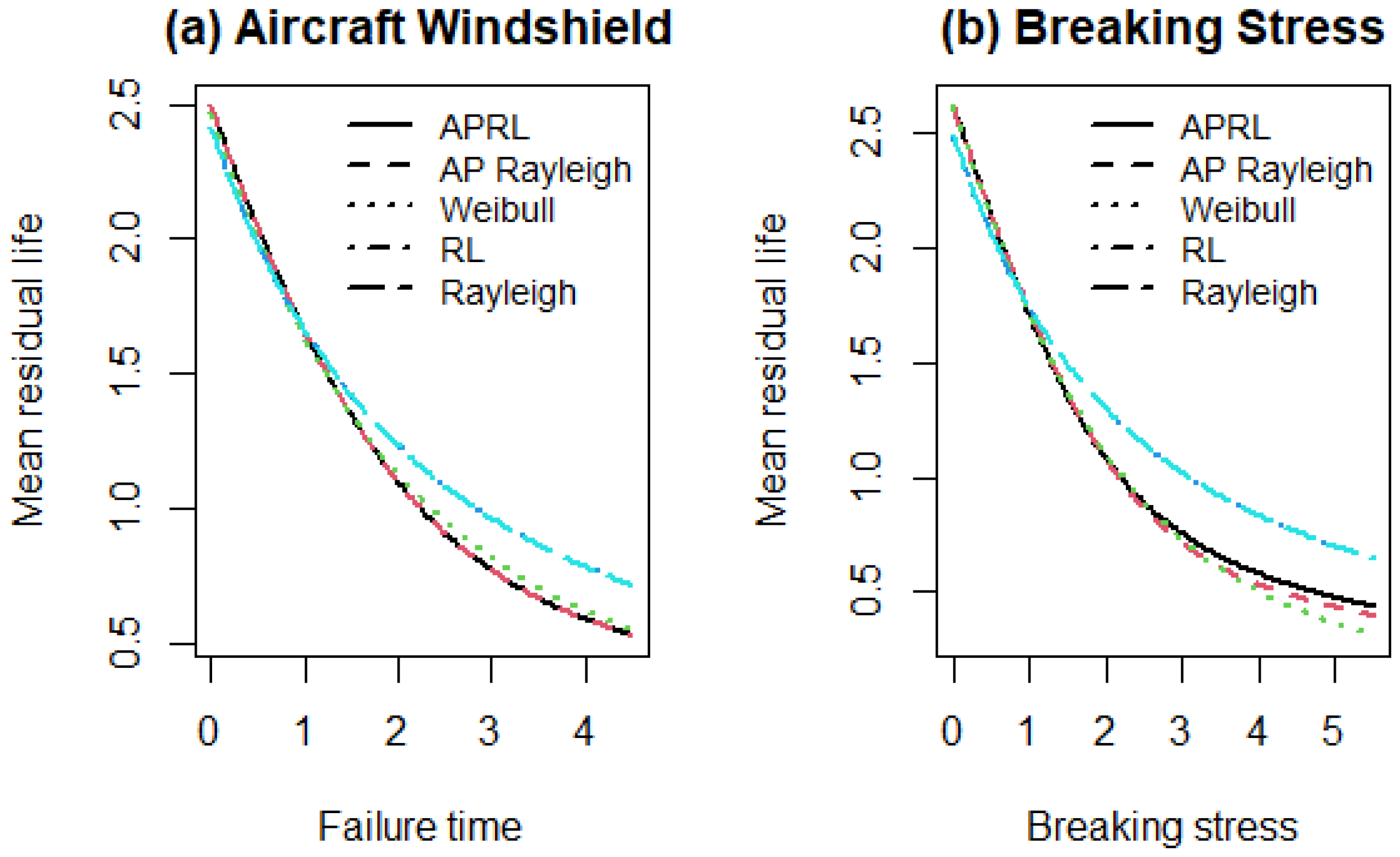
As shown in

Table 11. Estimated MTTF values for the fitted lifetime models.

Distribution	Aircraft Windshield MTTF	Breaking Stress MTTF
APRL	2.4957	2.6207
Alpha Power Rayleigh	2.4957	2.6173
Weibull	2.4661	2.6210
RL	2.4105	2.4892
Rayleigh	2.4105	2.4892

and Figure 14, the APRL model provides MTTF estimates comparable to those of the best-fitting competing models in both applications. In particular, the APRL and Alpha Power Rayleigh models yield nearly identical MTTF values for the Aircraft Windshield data, while the APRL estimate for the Breaking Stress data is very close to those of the Alpha Power Rayleigh and Weibull models. The MRL curves in Figure 13 further show a decreasing pattern for all fitted models, with the APRL model exhibiting remaining lifetime behaviour comparable to the competing distributions in both datasets. Together, these results demonstrate the practical applicability of the MTTF and MRL measures derived for the proposed APRL distribution.

7. Conclusions

In this study, a three-parameter Alpha Power Rayleigh–Logarithmic (APRL) distribution was introduced by incorporating the Alpha Power transformation into the classical Rayleigh–Logarithmic distribution. The additional transformation parameter provides greater control over the distributional shape, skewness, tail behaviour, and the rate of increase in the hazard function while preserving the underlying structure of the baseline model. The principal mathematical and reliability properties of the distribution were established, and maximum likelihood estimation was implemented using a multiple-start numerical optimization strategy to reduce sensitivity to initial values and the possibility of convergence to local optima.

The simulation results showed that the estimation accuracy of the parameters generally improves as the sample size increases, as reflected by reductions in bias, MSE, and RMSE. The parameters $p$ and ${\sigma }^2$ exhibited comparatively stable estimation behaviour, whereas the transformation parameter α\alphaα showed greater finite-sample variability, particularly under more extreme parameter configurations. These findings indicate that additional caution is required when interpreting estimates of the transformation parameter in small samples or near the boundaries of the parameter space.

The real data applications further demonstrated the practical performance of the APRL distribution. For the Aircraft Windshield Failure Times data, the APRL and Alpha Power Rayleigh models produced nearly identical fitted behaviour, with the estimate of the logarithmic parameter approaching its boundary, indicating that the additional logarithmic component contributed little for this dataset. For the Breaking Stress of Carbon Fibres data, the APRL model provided a competitive fit relative to the Weibull and Alpha Power Rayleigh distributions and several other lifetime models. Since the model parameters were estimated from the same data, parametric bootstrap KS p-values were used for goodness-of-fit assessment, while bootstrap standard errors and confidence intervals were employed to provide more reliable inference for parameters close to the boundaries.

The practical relevance of the derived reliability measures was also examined through MTTF and MRL analyses. The APRL model produced MTTF estimates comparable to those of the best-fitting competing models in both applications, while the MRL curves exhibited decreasing remaining lifetime behaviour and were generally comparable with those of the competing distributions. These results complement the conventional goodness-of-fit criteria by demonstrating how the theoretical reliability measures of the APRL distribution can be interpreted in real lifetime applications.

The proposed model nevertheless has some limitations. Estimation of the transformation parameter can become more variable for extreme parameter values and small samples, and boundary estimates may occur in real data applications. Moreover, the present inference framework is restricted to complete lifetime data and maximum likelihood estimation. Future research may therefore consider censored and truncated lifetime data, regression formulations, Bayesian and robust estimation procedures, and additional diagnostic methods specifically designed for the APRL distribution. Such developments may extend its applicability in reliability and survival modelling.

References

1. Adamidis, K.; Loukas, S. A Lifetime Distributions with Decreasing Failure Rate. Stat. Probab. Lett. 1998, 39, 35–42. [Google Scholar] [CrossRef]
2. Kus, C. A New Lifetime Distribution. Comput. Stat. Data Anal. 2007, 51, 4497–4509. [Google Scholar] [CrossRef]
3. Lu, W.; Shi, D.A. New Compounding Life Distribution: The Weibull-Poisson Distribution. J. Appl. Stat. 2011, 39, 21–38. [Google Scholar] [CrossRef]
4. Bakouch, H.S.; Jazi, M.A.; Nadarajah, S.; Dolati, A.A. Lifetime Model with Increasing Failure Rate. Appl. Math. Model. 2014, 38, 5392–5406. [Google Scholar] [CrossRef]
5. Mahdavi, A.; Kundu, D. A new method for generating distributions with an application to exponential distribution. Commun. Stat.-Theory Methods 2017, 46, 6543–6557. [Google Scholar] [CrossRef]
6. Dey, S.; Alzaatreh, A.; Zhang, C.; Kumar, D. A new extension of generalized exponential distribution with application to Ozone data. Ozone Sci. Eng. 2017, 39, 273–285. [Google Scholar] [CrossRef]
7. Ahmet, M.A. On the Alpha Power Kumaraswamy Distribution: Properties, Simulation and Application. Rev. Colomb. Estad.-Appl. Stat. 2020, 43, 285–313. [Google Scholar] [CrossRef]
8. Dey, S.; Ghosh, I.; Kumar, D. Alpha-Power Transformed Lindley Distribution: Properties and Associated Inference with Application to Earthquake Data. Ann. Data Sci. 2019, 6, 623–650. [Google Scholar] [CrossRef]
9. Eghwerido, J.T. The alpha power Teissier distribution and its applications. Afr. Stat. 2021, 16, 2733–2747. [Google Scholar] [CrossRef]
10. Aldahlan, M.A. Alpha Power Transformed Log-Logistic Distribution with Application to Breaking Stress Data. Adv. Math. Phys. 2020, 2020, 2193787. [Google Scholar] [CrossRef]
11. Nassar, M.; Alzaatreh, A.; Mead, M.; Abo-Kasem, O. Alpha power weibull distribution: Properties and applications. Commun. Stat.-Theory Methods 2017, 46, 10236–10252. [Google Scholar] [CrossRef]
12. Basheer, A.M. Alpha power inverse Weibull distribution with reliability application. J. Taibah Univ. Sci. 2019, 13, 423–432. [Google Scholar] [CrossRef]
13. Kızılkaya, H. Alfa Power Transformed Rayleigh Distribution. Master’s Thesis, Institute of Science, Kırıkkale University, Kırıkkale, Türkiye, 2021. [Google Scholar]
14. Tekin, S.; Ozel, G. Alfa Power Burr-XII Distribution and An Application. J. Quant. Sci. 2020, 2, 33–46. [Google Scholar]
15. Unal, C.; Cakmakyapan, S.; Ozel, G. Alpha power inverted exponential distribution: Properties and application. Gazi Univ. J. Sci. 2018, 31, 954–965. [Google Scholar]
16. Hassan, A.S.; Mohamd, R.E.; Elgarhy, M.; Fayomi, A. Alpha power transformed extended exponential distribution: Properties and applications. J. Nonlinear Sci. Appl. 2018, 12, 62–67. [Google Scholar] [CrossRef]
17. Mead, M.E.; Cordeiro, G.M.; Afify, A.Z.; Al-Mofleh, H. The alpha power transformation family: Properties and applications. Pak. J. Stat. Oper. Res. 2019, 15, 525–545. [Google Scholar] [CrossRef]
18. Ihtisham, S.; Khalil, A.; Manzoor, S.; Khan, S.A.; Ali, A. Alpha-Power Pareto distribution: Its properties and applications. PLoS ONE 2019, 14, e0218027. [Google Scholar] [CrossRef] [PubMed]
19. Martinez-Florez, G.; Tovar-Falon, R.; Jimemez-Narvaez, M. Likelihood-Based Inference for the Asymmetric Beta-Skew Alpha-Power Distribution. Symmetry 2021, 12, 613. [Google Scholar] [CrossRef]
20. Ijaz, M.S.; Asim, M.; Farooq, A.M.; Khan, S.A.; Manzoor, S. A Gull Alpha Power Weibull distribution with applications to real and simulated data. PLoS ONE 2020, 15, e0233080. [Google Scholar] [CrossRef] [PubMed]
21. Eghwerido, J.T.; Nzei, L.C.; Agu, F.I. The Alpha Power Gompertz Distribution: Characterization, Properties, and Applications. Sankhya A 2021, 83, 449–475. [Google Scholar] [CrossRef]
22. Bleed, S.O.; Attwa, R.A.E.; Ali, R.F.M.; Radwan, T. On alpha power transformation generalized pareto distribution and some properties. J. Appl. Math. 2024, 2024, 6270350. [Google Scholar] [CrossRef]
23. Méndez-González, L.C.; Rodríguez-Picón, L.A.; Pérez-Olguin, I.J.C.; Garcia, V.; Quezada-Carreón, A.E. A reliability analysis for electronic devices under an extension of exponentiated perks distribution. Qual. Reliab. Eng. Int. 2023, 39, 776–795. [Google Scholar] [CrossRef]
24. Musekwa, R.R.; Gabaitiri, L.; Makubate, B. A new family of bivariate alpha log power transformation model based on extreme shock models. Stat. Optim. Inf. Comput. 2016, 15, 1463–1479. [Google Scholar]
25. Kawo, K.N.; Goshu, A.T.; Kindo, B.P. A New Alpha Power Transformation of Logistic Distribution with Its Properties and Applications. J. Probab. Stat. 2025, 2025, 9594412. [Google Scholar] [CrossRef]
26. Aliabadi, M.; Ghatari, A.H.; Khorram, E. A Three-Parameter Alpha Power Erlang Distribution for Modeling Lifetime Data. Stat. Optim. Inf. Comput. 2025, 14, 2208–2227. [Google Scholar] [CrossRef]
27. Alghamdi, A.S.; ALoufi, S.F.; Baharith, L.A. The sine alpha power-g family of distributions: Characterizations, regression modeling, and applications. Symmetry 2025, 17, 468. [Google Scholar] [CrossRef]
28. Abiad, M.; Khan, N.S.; Shafiq, M.; ul Haq, I. An Extended Alpha Power Family of Distributions: Its Applications to the Scientific Data. Int. J. Anal. Appl. 2025, 23, 134. [Google Scholar] [CrossRef]
29. Bugatekin, A. A new distribution model with two-parameter. New Trends Math. Sci. 2017, 5, 80–84. [Google Scholar] [CrossRef]
30. Hameed, A.F.; Alwan, I.M. Bayes estimators for reliability and hazard function of Rayleigh-Logarithmic (RL) distribution with application. Period. Eng. Nat. Sci. 2020, 8, 1991–1998. [Google Scholar] [CrossRef]
31. Tahir, M.H.; Cordeiro, G.M.; Mansoor, M.; Zubair, M. The Weibull–Lomax Distribution: Properties and Applications. Hacet. J. Math. Stat. 2015, 44, 455–474. [Google Scholar] [CrossRef]
32. Nichols, M.D.; Padgett, W.J. A Bootstrap Control Chart for Weibull Percentiles. Qual. Reliab. Eng. Int. 2006, 22, 141–151. [Google Scholar] [CrossRef]
Figure 1. Histograms and theoretical probability density functions (pdfs) of the APRL distribution for different α values (1.1, 2, 5, 10, 20). Parameters: p = 0.5, σ 2 = 2.
Appliedmath 06 00128 g001
Figure 2. Probability density function of the APRL distribution for different parameter values.
Appliedmath 06 00128 g002
Figure 3. Survival and hazard rate functions of the APRL distribution for different values of the shape parameter α , with p = 0.7 and σ 2 = 0.5 .
Appliedmath 06 00128 g003
Figure 4. Mean residual life functions of the APRL distribution under different values of the shape parameter α and the scale parameter σ 2 .
Appliedmath 06 00128 g004
Figure 5. Quantile function of the APRL distribution for the selected parameter values.
Appliedmath 06 00128 g005
Figure 6. Plots of the S k and M k for various parameter settings of the APRL distribution.
Appliedmath 06 00128 g006
Figure 7. RMSE values of the maximum likelihood estimators of α , p , and σ 2 as functions of the sample size under the four parameter configurations considered in Table 3, Table 4, Table 5 and Table 6. All results are based on R = 300 Monte Carlo replications.
Appliedmath 06 00128 g007
Figure 8. Graphical goodness-of-fit diagnostics for the fitted APRL distribution for the Aircraft Windshield Failure Times data: Q–Q plot and P–P plot.
Appliedmath 06 00128 g008
Figure 9. Fitted density curves of the APRL and competing lifetime distributions for the Aircraft Windshield Failure Times data.
Appliedmath 06 00128 g009
Figure 10. Fitted reliability and hazard rate functions of the APRL, Alpha Power Rayleigh, and Weibull distributions for the Aircraft Windshield Failure Times data.
Appliedmath 06 00128 g010
Figure 11. Graphical goodness-of-fit diagnostics for the fitted APRL distribution for the Breaking Stress of Carbon Fibres data: Q–Q plot and P–P plot.
Appliedmath 06 00128 g011
Figure 12. Fitted density curves of the APRL and competing lifetime distributions for the Breaking Stress of Carbon Fibres data.
Appliedmath 06 00128 g012
Figure 13. Fitted reliability and hazard rate functions of the APRL, Alpha Power Rayleigh, and Weibull distributions for the Aircraft Windshield Failure Times data.
Appliedmath 06 00128 g013
Figure 14. Mean residual life (MRL) curves of the fitted lifetime models for (a) the Aircraft Windshield Failure Times data and (b) the Breaking Stress of Carbon Fibres data.
Appliedmath 06 00128 g014