Modeling and Dynamical Analysis of a Fractional-Order Predation Model Incorporating Disease and Cooperative Hunting

Abstract

This study constructs a novel fractional-order eco-epidemiological predator–prey model, in which disease spreads among predators through environmental transmission, and both cooperative hunting behavior and disease latency delay are incorporated simultaneously. Different from classical integer-order predator–prey models, fractional derivative is adopted to describe the memory-dependent mechanism of ecological populations, and the infection can alter the hunting strategy of diseased predators. The existence, non-negativity, and boundedness of system solutions are proved theoretically. The local stability of all equilibrium points is analyzed, and the conditions for the occurrence of Hopf bifurcation induced by latency delay are derived. Numerical simulations further verify the theoretical results, and quantitatively reveal the separate and combined effects of the fractional order, cooperative hunting coefficient, and latency delay on the dynamical evolution of the population system.

1. Introduction

In the field of biomathematics, population dynamics and infectious diseases have received considerable attention [1,2,3]. In recent years, several outbreaks of infectious diseases, such as HIV/AIDS, COVID-19, Japanese encephalitis [4], and other widespread infectious diseases, have occurred. These diseases are harmful and pose a threat to the lives and health of individuals worldwide. Therefore, the prevention and control of infectious diseases have become top priorities. In response to the growing threat of infectious diseases, many mathematical researchers have devoted themselves to studying these diseases and have built mathematical models to analyze their transmission mechanisms [5,6]. While it is important to focus on diseases that affect humans, it is equally important to pay attention to infectious diseases in animals, known as eco-epidemics. The spread of a disease in a wild animal population is also known as a wildlife epidemic. Examples of such diseases include the Ebola virus, avian influenza, and tularemia. Some ecological epidemics can cross species boundaries and infect humans, resulting in zoonotic infections [7,8]. These cross-species infections present unique challenges in disease management and prevention. Because predation is the most common relationship between populations, mathematicians naturally combine predation systems with ecological epidemiology to analyze mathematical results [9,10,11].

The transmission of infectious diseases involves numerous factors, of which the environment plays a particularly vital role. Environmental transmission refers to the spread and persistence of pathogens in the environment [12,13,14]. In ecological epidemics, pathogens are often closely associated with the natural habitats of wild animals, including factors such as habitat, climate, and geographical conditions [15,16]. Pathogens can be transmitted in the environment through various means, including the feces, urine, saliva, and respiratory secretions of infected wild animals. Direct or indirect contact between infected animals and environmental elements such as water, soil, and vegetation can also facilitate transmission. White-nose syndrome (WNS) is a disease that primarily affects bats [17]. It is caused by the fungus Pseudogymnoascus destructans, which forms white patches on the nose, wings, and skin of bats, compromising their immune system and causing severe health problems. WNS, which was initially discovered in North America, caused significant bat mortality within a short period [18]. The spread of this disease is closely linked to environmental factors, including specific temperature and humidity conditions within bat habitats as well as the swarming behavior of bats [17]. Therefore, eco-epidemiological research should focus on studying the interactions between the environment and animals to gain insights into the transmission mechanisms of diseases and to assess the associated risks. However, existing research on eco-epidemic diseases often overlooks the role of environmental infections in transmission mechanisms.

Cooperative hunting, in which predators work together to attack prey, is a strategic behavior that is observed in many animal species, such as wolves, lemurs, and sharks. This behavior not only highlights the sociality of animals, but also plays a crucial role in shaping the ecosystem stability and population dynamics of other species. Therefore, cooperative hunting in predation systems has attracted extensive attention from scholars [19,20,21]. However, previous research has primarily focused on healthy populations, and few studies have explored the impact of disease on cooperative hunting. Although the authors in [22,23] considered both cooperative hunting and disease, they mainly considered prey disease and did not consider the relationship between predator disease and cooperative hunting. In reality, when some animals contract infectious diseases, they often self-isolate, are ostracized, or consciously leave the group [24]. Particularly in group-living populations, these diseased individuals are typically excluded from cooperative hunting activities. One possible explanation is that healthy individuals avoid contact with sick individuals to mitigate the risk of disease transmission. To understand the relationship between disease and cooperative hunting comprehensively, it is essential to consider the influence of disease on cooperative hunting behavior. Research in this area can provide valuable insights into disease transmission and animal behavior while concurrently enhancing our understanding of ecosystem dynamics and population interactions.

When investigating intricate dynamical behaviors inherent to natural ecosystems, instantaneous system states are governed jointly by contemporary environmental conditions and preceding historical evolutions. Such temporal dependency renders conventional integer-order differential models inadequate to characterize long-range memory and nonlocal interactions across ecological systems. As a generalized extension of classical integer-order calculus, fractional calculus is endowed with a prominent merit: its inherent memory-kernel framework is capable of quantifying the hereditary properties of dynamical systems and accurately depicting cumulative historical impacts embedded within ecological evolution [25]. In recent years, research on fractional calculus has made unprecedented progress [26,27,28,29,30,31]. Fractional calculus has a property between integer-order differential and integral stochastic processes, which can describe the phenomena of non-stationary, nonlinear, and long-term memory more accurately. Fractional calculus has a wider range of applications than integral calculus, such as signal processing [27], image recognition [28], financial engineering [29], and medical diagnosis [30,31]. Particularly in ecology, many scholars have used fractional-order systems to model populations and infectious diseases, and several results have been obtained [32,33,34]. However, among the numerous studies on fractional infectious diseases, most still focus on disease transmission of diseases among humans, while few have specifically studied the impact of diseases on population survival.

In many real-world problems, the system response may depend on past states or inputs, and ignoring this information can lead to false predictions of the system behavior. Therefore, an increasing number of researchers have begun to pay attention to delay differential equations [35,36]. This approach can reflect the historical evolution of a system and provide more accurate predictions and modeling capabilities, and is therefore favored by many mathematicians. Particularly in the field of fractional calculus, the corresponding fractional delay differential equations have been established [37,38]. Time delay can lead to switching of the equilibrium stability of the system and result in richer dynamic behavior. In addition, research on Hopf bifurcation has attracted much attention in recent years; in particular, the time delay is generally preferred as the bifurcation parameter [39,40,41].

Inspired by the above research and to fill the gaps in the current research, we propose a new mathematical model to better understand the impact of disease on population dynamics in ecological epidemiology. The main contributions of this study are as follows:

(1)

A fractional-order predation model that considers environmental infection is established for the first time, and the effect of disease on cooperative hunting is proposed.

(2)

By adopting the Caputo fractional derivative, this work establishes a novel fractional eco-epidemiological model, which overcomes the drawbacks of integer-order counterparts via characterizing system memory and hereditary population dynamics.

(3)

Considering the delay in disease transmission, the Hopf bifurcation criterion caused by the delay of disease latency is discussed.

2. Model Description and Preliminaries

Cooperative hunting constitutes a widely investigated predation strategy within eco-epidemiological modeling [22,23,41]. As a representative work, Saha et al. [22] constructed a predator–prey system featuring infected prey and cooperative predation behavior of predators:

$$\begin{array}{cc}& {\displaystyle \frac{dS}{dt}}={\displaystyle \frac{rS}{1+k_{1}y}}-dS-a{S}^2-{\displaystyle \frac{\beta SI}{1+k_{2}y}},\hfill \\ & {\displaystyle \frac{dI}{dt}}={\displaystyle \frac{\beta SI}{1+k_{2}y}}-\delta I-(p+by)Iy,\hfill \\ & {\displaystyle \frac{dy}{dt}}=c(p+by)Iy-my,\hfill \end{array}$$

(1)

where S and I represent the population densities of susceptible and infected prey, respectively. y represents the density of predators. Liu et al. [23] developed an eco-epidemiological model incorporating fear effect and cooperative hunting among predators:

$$\begin{array}{cc}\hfill {\displaystyle \frac{\mathrm{d}X}{\mathrm{d}t}}& =rX\left(1-{\displaystyle \frac{X}{K}}\right)-{\beta }_{1}XY-{\displaystyle \frac{AXZ}{1+T_{h}A{X}^2}},\hfill \\ \hfill {\displaystyle \frac{\mathrm{d}Y}{\mathrm{d}t}}& ={\beta }_{1}XY-\zeta \left(1+{\alpha }_{1}Z\right)YZ-{\delta }_{1}Y,\hfill \\ \hfill {\displaystyle \frac{\mathrm{d}Z}{\mathrm{d}t}}& ={\displaystyle \frac{c_{1}AXZ}{1+T_{h}A{X}^2}}+{\xi }_1\zeta \left(1+{\alpha }_{1}Z\right)YZ-{\eta }_{1}Z,\hfill \end{array}$$

(2)

where $X,Y$ and Z represent susceptible prey, infected prey and predator, respectively. Both systems (1) and (2) incorporate disease infection within prey populations but neglect pathogenic infection in predators. To remedy this limitation, Hilker et al. [41] constructed a model accounting for predator disease as well as intraspecific cooperative predation:

$$\begin{array}{cc}& {\displaystyle \frac{\mathrm{d}N}{\mathrm{d}t}}=r\left(1-{\displaystyle \frac{N}{K}}\right)N-\left(a_0+a_{1}P\right)NP,\hfill \\ & {\displaystyle \frac{\mathrm{d}S}{\mathrm{d}t}}=-\beta {\displaystyle \frac{SI}{P}}-mS+ϵ\left(a_0+a_{1}P\right)NS+(1-\theta )ϵ\left(a_0+a_{1}P\right)NI,\hfill \\ & {\displaystyle \frac{\mathrm{d}I}{\mathrm{d}t}}=\beta {\displaystyle \frac{SI}{P}}-mI-\mu I+\theta ϵ\left(a_0+a_{1}P\right)NI,\hfill \end{array}$$

(3)

where $N,S$ and I represent the density of prey, susceptible predator populations and infected predator populations, respectively. System (3) focuses on the effects of density-mediated disease, but does not consider the effects of traits such as whether the disease affects the group hunting behavior of infected predators. Sick predators often voluntarily leave the group or are forcibly excluded from a group of uninfected predators [24]. An animal’s internal self-protection mechanism plays a key role in this phenomenon. In addition, it is necessary to consider the transmission of diseases through the environment. Many studies have shown that factors such as animal feces and contaminated water sources can indirectly spread diseases [15,16,17]. Therefore, significant attention must be paid to this key factor of environmental transmission. However, the existing research has obvious deficiencies in this aspect.

Based on the above analysis and works, we propose a PP model with cooperative hunting and environmental infection. For the purposes of this study, we make the following assumptions:

(i)

The disease is transmitted only between predators.

(ii)

Infected predators do not recover from the disease and are voluntarily or passively excluded from group life.

(iii)

Infected predators do not participate in cooperative hunting and can only hunt for food on their own.

(iv)

The strains in the environment all originate from infected predators.

Finally, the governing mathematical model is formulated as below:

$$\begin{array}{cc}& {\displaystyle \frac{dx}{dt}}=rx(1-{\displaystyle \frac{x}{k}})-(\alpha +\gamma y_s)x{y}_s-\eta x{y}_i-dx,\hfill \\ & {\displaystyle \frac{d{y}_s}{dt}}=e(\alpha +\gamma y_s)x{y}_s-\theta y_s{y}_i(t)-\mu y_{s}z(t)-d_1{y}_s,\hfill \\ & {\displaystyle \frac{d{y}_i}{dt}}=f\eta x{y}_i+\theta y_s{y}_i(t)+\mu y_{s}z(t)-d_2{y}_i,\hfill \\ & {\displaystyle \frac{dz}{dt}}=\phi y_i-\epsilon z,\hfill \end{array}$$

(4)

where x represents prey, $y_s$ represents susceptible predators, $y_i$ is infected predators, and z is the number of pathogens in the environment. All parameter definitions for system (4) are summarized in

Table 1. Biological meaning of the variables and parameters for system (4).

r	Intrinsic growth rate of prey
k	Environmental carrying capacity of prey
$\alpha$	The capture rate of susceptible predators
$\gamma$	Cooperative hunting coefficient among susceptible predators
$\eta$	The capture rate of infected predators
e	The conversion rate of susceptible predators to prey
f	The conversion rate of infected predators to prey
$\theta$	The incidence of disease among predators
$\phi$	Number of viruses in the environment
$\mu$	The incidence of diseases exposed to infected environments
d	The death rate of prey
$d_1$	The death rate of susceptible predators
$d_2$	The death rate of infected predators
$\epsilon$	The natural death rate of the virus
$\tau$	The latency of the disease

.

Since the initial conditions of Caputo fractional differential equations are consistent with those of integer-order differential equations, this definition intuitively aligns with the physical connotation of memory effects in biological systems and can effectively characterize the historical dependence and hereditary properties of dynamical systems [37]. Accordingly, this paper introduces the Caputo fractional derivative into system (4) and further investigates the disease incubation period $\tau$ based on the improved model. The resulting fractional-order system is expressed as follows:

$$\begin{array}{cc}& {}_{t_0}{}^{C }D_t^{\varrho }x(t)=rx(1-{\displaystyle \frac{x}{k}})-(\alpha +\gamma y_s)x{y}_s-\eta x{y}_i-dx,\hfill \\ & {}_{t_0}{}^{C }D_t^{\varrho }{y}_s(t)=e(\alpha +\gamma y_s)x{y}_s-\theta y_s{y}_i(t-\tau )-\mu y_{s}z(t-\tau )-d_1{y}_s,\hfill \\ & {}_{t_0}{}^{C }D_t^{\varrho }{y}_i(t)=f\eta x{y}_i+\theta y_s{y}_i(t-\tau )+\mu y_{s}z(t-\tau )-d_2{y}_i,\hfill \\ & {}_{t_0}{}^{C }D_t^{\varrho }z(t)=\phi y_i-\epsilon z.\hfill \end{array}$$

(5)

The initial conditions for system (5) are as follows:

$$x(\varpi )>0,y_s(\varpi )>0,y_i(\varpi )>0,z(\varpi )>0for\varpi \in [-\tau ,0].$$

(6)

Remark 1.

The parameters e and f denote the biomass conversion efficiencies of susceptible and infected predators from consumed prey, respectively. From a biological perspective, part of the prey biomass consumed is dissipated via metabolism and respiration rather than converted into predator population growth, which yields $0<e<1$ and $0<f<1$.

Some necessary definitions and lemmas required throughout this study are presented below.

Definition 1

([26]). The Caputo fractional derivative is defined by

$${}_{t_0}{}^{C }D_t^{\varrho }f(t)={\displaystyle \frac{1}{\Gamma (n-\varrho )}}{\int }_{t_0}^t{(t-\tau )}^{n-\varrho -1}{f}^n(\tau )d\tau ,$$

where n is a positive integer, and $n-1<\varrho <n$, $\Gamma (·)$ is the Gamma function with $\Gamma (s)={\int }_0^{\infty }{t}^{s-1}{e}^{-t}dt$.

Definition 2

([42]). The Laplace transform of Caputo fractional-order derivative is

$$\pounds \left\{{}_{t_0}{}^{C }D_t^{\varrho }f(t);s\right\}=s^{\varrho }F(s)-{\displaystyle \sum _{i=0}^{n-1}}{s}^{\varrho -i-1}{f}^{(i)}(t_0),$$

where $F(s)=\pounds \{f(t)\}$. In particular, when $f^{(i)}(t_0)=0,i=1,2,\dots ,n-1$, then

$$\pounds \left\{{}_{t_0}{}^{C }D_t^{\varrho }f(t);s\right\}=s^{\varrho }F(s).$$

Lemma 1

([43]). Let $f(t)$ be a continuous function on $\left[t_0,+\infty \right)$ and satisfying

$$\left\{\begin{array}{c}{}_{t_0}{}^{C }D_t^{\varrho }f(t)\le -\lambda f(t)+\mu ,\hfill \\ f\left(t_0\right)=f_{t_0},\hfill \end{array}\right.$$

where $0<\varrho <1,(\lambda ,\mu )\in {\mathbb{R}}^2$ and $\lambda \ne 0$, and $t_0\ge 0$ is the initial time. Then

$$f(t)\le \left(f_{t_0}-{\displaystyle \frac{\mu }{\lambda }}\right)E_{\varrho }\left[-\lambda {\left(t-t_0\right)}^{\varrho }\right]+{\displaystyle \frac{\mu }{\lambda }}.$$

3. Existence, Nonnegativity, and Boundedness of Solutions

In this section, we investigate the existence, nonnegativity, and uniform boundedness of solutions to system (5).

Theorem 1.

System (5) admits a unique solution satisfying the initial condition (6).

Proof. 

First, consider a region $\mathsf{\Psi }\times (t_0,T)$, $T<\infty$, where $\mathsf{\Psi }=\{(x,y_s,y_i,z)\in R^4,$$max\mid x\mid ,\mid y_s\mid ,\mid y_i\mid ,\mid z\mid \le \zeta \}$. Then, let us consider a map

$$\Re (Y)=({\Re }_1(Y),{\Re }_2(Y),{\Re }_3(Y),{\Re }_4(Y)),$$

where $Y=(x,y_s,y_i,z)$ and $\hat{Y}=(\hat{x},{\hat{y}}_s,{\hat{y}}_i,\hat{z})$.

$$\begin{array}{cc}\hfill & {\Re }_1(Y)=rx(1-{\displaystyle \frac{x}{k}})-(\alpha +\gamma y_s)x{y}_s-\eta x{y}_i-dx,\hfill \\ \hfill & {\Re }_2(Y)=e(\alpha +\gamma y_s(t))x{y}_s-\theta y_s{y}_i(t-\tau )-\mu y_{s}z(t-\tau )-d_1{y}_s,\hfill \\ \hfill & {\Re }_3(Y)=f\eta x{y}_i+\theta y_s{y}_i(t-\tau )+\mu y_{s}z(t-\tau )-d_2{y}_i,\hfill \\ \hfill & {\Re }_4(Y)=\phi y_i-\epsilon z.\hfill \end{array}$$

For any $Y,\hat{Y}\in \mathsf{\Psi },$ we have

$$\begin{array}{cc}\hfill & \parallel \Re (Y)-\Re (\hat{Y})\parallel \hfill \\ \hfill =& |{\Re }_1(Y)-{\Re }_1(\hat{Y})|+|{\Re }_2(Y)-{\Re }_2(\hat{Y})|+|{\Re }_3(Y)-{\Re }_3(\hat{Y})|+|{\Re }_4(Y)-{\Re }_4(\hat{Y})|\hfill \\ \hfill =& \mid rx(1-{\displaystyle \frac{x}{k}})-(\alpha +\gamma y_s)x{y}_s-\eta x{y}_i-dx-[r\hat{x}(1-{\displaystyle \frac{\hat{x}}{k}})-(\alpha +\gamma \widehat{y_s})\hat{x}\widehat{y_s}\hfill \\ \hfill & -\eta \hat{x}\widehat{y_i}-d\hat{x}]\mid +\mid e(\alpha +\gamma y_s)x{y}_s-\theta y_s{y}_i(t-\tau )-\mu z(t-\tau )y_s-d_1{y}_s-[e(\alpha +\gamma \widehat{y_s})\hat{x}\widehat{y_s}\hfill \\ \hfill & -\theta \widehat{y_s}\widehat{y_i}(t-\tau )-\mu \hat{z}(t-\tau )\widehat{y_s}-d_1\widehat{y_s}]\mid +\mid f\eta x{y}_i+\theta y_s{y}_i(t-\tau )+\mu z(t-\tau )y_s-d_2{y}_i\hfill \\ \hfill & -[f\eta \hat{x}{y}_i+\theta \widehat{y_s}\widehat{y_i}(t-\tau )+\mu \hat{z}(t-\tau )\widehat{y_s}-d_2\widehat{y_i}]\mid +\mid \phi y_i-\epsilon z-[\phi \widehat{y_i}-\epsilon \hat{z}]\mid \hfill \\ \hfill \le & [r+{\displaystyle \frac{2\zeta r}{k}}+(e+1)(\alpha \zeta +\gamma {\zeta }^2)+(f+1)\eta \zeta +d]\mid x-\hat{x}\mid \hfill \\ \hfill & +[(e+1)(\alpha \zeta +2\gamma {\zeta }^2)+2\zeta (\theta +\mu )+d_1]\mid y_s-{\hat{y}}_s\mid \hfill \\ \hfill & +[\zeta (2\eta +\theta +f\eta )+d_2+\phi ]\mid y_i-{\hat{y}}_i\mid +[2\mu \zeta +\epsilon ]\mid z-\hat{z}\mid \hfill \\ \hfill & ={\mathsf{\ell }}_1\mid x-\hat{x}\mid +{\mathsf{\ell }}_2\mid y_s-{\hat{y}}_s\mid +{\mathsf{\ell }}_3\mid y_i-{\hat{y}}_i\mid +{\mathsf{\ell }}_4\mid z-\hat{z}\mid \hfill \\ \hfill \le & \mathsf{\ell }\parallel Y-\hat{Y}\parallel ,\hfill \end{array}$$

where $\mathsf{\ell }=max\{{\mathsf{\ell }}_1,{\mathsf{\ell }}_2,{\mathsf{\ell }}_3,{\mathsf{\ell }}_4\}.$ Accordingly, $\Re (Y)$ satisfies the local Lipschitz condition, which verifies the validity of the desired theorem. □

Theorem 2.

If $d_2>\phi$, then all positive initial-value solutions of system (5) defined on ${\mathbb{R}}_{+}^4$ remain nonnegative and are uniformly ultimately bounded in the region

$$\Omega =\left\{(x,y_s,y_i,z)\in R_{+}^4\mid 0<\aleph (t)\le {\displaystyle \frac{kr}{4\Lambda }}+ϵ,ϵ>0\right\}.$$

Proof. 

First, we verify the nonnegativity of all system solutions. Let the initial state satisfy $(x(t_0),y_s(t_0),y_i(t_0),z(t_0))\in {\mathbb{R}}_{+}^4$. We adopt contradiction to verify $x(t)\ge 0,y_s(t)\ge 0,y_i(t)\ge 0,z(t)\ge 0$ for all $t\ge t_0$. We first prove the nonnegativity of $x(t)$ for all $t\ge t_0$. The first equation can be written as:

$${}_{t_0}{}^{C }D_t^{\varrho }x(t)=x(t)M(t),$$

where

$$M_1(t)=r\left(1-{\displaystyle \frac{x(t)}{k}}\right)-(\alpha +\gamma y_s(t))y_s(t)-\eta y_i(t)-d.$$

From the existence and uniqueness of solutions (Theorem 1), all state variables $x(t),y_s(t),$$y_i(t),z(t)$ are continuous and bounded on any finite interval $[t_0,T]$. Therefore, $M(t)$ is continuous and bounded on $[t_0,T]$. From the biological context of the model, the parameters satisfy: $r>0, k>0, d>0, \alpha >0, \gamma >0, \eta >0$.

Then on any finite interval $[t_0,T]$, we have:

$$M_1(t)\ge -r{\displaystyle \frac{y_{max}}{k}}-(\alpha +\gamma y_{max})y_{max}-\eta y_{max}-d,$$

where $y_{max}$ is an upper bound for $x(t),y_s(t),y_i(t)$. Thus, there exists a constant $M_1\in \mathbb{R}$ such that $M_1(t)\ge M_1$ for all $t\in [t_0,T]$. Based on the comparison principle for Caputo fractional differential inequalities (Lemma 3.4 in Ref. [43]) and the initial condition $x(t_0)>0$, we derive

$$x(t)\ge x(t_0)E_{\varrho }\left[M_1{(t-t_0)}^{\varrho }\right]>0,\forall t\in [t_0,T].$$

Since T is arbitrary, $x(t)\ge 0$ for all $t\ge t_0$.

Since $x(t)$ is positive, we turn to the second equation of system (5), yielding

$${}_{t_0}{}^{C }D_t^{\varrho }{y}_s(t)=\gamma y_s^2(t)x(t)+\left[e\alpha x(t)-\theta y_i(t-\tau )-\mu z(t-\tau )-d_1\right]y_s(t)\ge M_2(t),$$

where

$$M_2(t)=\left[e\alpha x(t)-\theta y_i(t-\tau )-\mu z(t-\tau )-d_1\right]y_s(t).$$

On $[t_0,T]$, $x(t),y_s(t),y_i(t),z(t)$ are bounded continuous, so there exists a constant $M_2\in \mathbb{R}$ such that $M_2(t)\ge M_2$ for all $t\in [t_0,T]$. With the positive initial history $y_s(\varpi )>0$ defined over the delay interval $[-\tau ,0]$, we employ the fractional comparison principle tailored to delay differential equations of Caputo type:

$$y_s(t)\ge y_s(t_0)E_{\varrho }\left(M_2{(t-t_0)}^{\varrho }\right)>0,\forall t\in [t_0,T].$$

Arbitrariness of T gives $y_s(t)>0,\forall t\ge t_0$.

From the second equation of system (5), we obtain

$${}_{t_0}{}^{C }D_t^{\varrho }{y}_i(t)=\left[f\eta x(t)-d_2\right]y_i(t)+\theta y_s(t)y_i(t-\tau )+\mu y_s(t)z(t-\tau ).$$

Let $M_i(t)=f\eta x(t)-d_2,S_i(t)=\theta y_s(t)y_i(t-\tau )+\mu y_s(t)z(t-\tau )\ge 0.$

Then we have a linear fractional delay inequality:

$${}_{t_0}{}^{C }D_t^{\varrho }{y}_i(t)-M_i(t)y_i(t)=S_i(t)\ge 0.$$

On $[t_0,T]$, $M_i(t)$ is bounded below by some constant $M_{i,\mathrm{low}}\in \mathbb{R}$. The history function satisfies $y_i(\varpi )>0,\varpi \in [-\tau ,0]$. By the positivity invariance theorem for Caputo fractional delay ODEs: if the forcing term $S_i(t)\ge 0$ and initial history is positive, then $y_i(t)>0,$$\forall t\in [t_0,T].$ Thus, $y_i(t)>0$ for all $t\ge t_0$.

Lastly, we verify the positivity of $z(t)$. Consider the fourth equation of system (5):

$${}_{t_0}{}^{C }D_t^{\varrho }z(t)+\epsilon z(t)=\phi y_i(t).$$

From previous analysis, $y_i(s)>0$ holds for all $s\ge t_0$, so the forcing term $\phi y_i(t)$ is strictly positive over the entire time domain. The analytical solution of this linear fractional equation reads

$$z(t)=z(t_0)E_{\varrho }\left(-\epsilon {(t-t_0)}^{\varrho }\right)+\phi {\int }_{t_0}^t{(t-s)}^{\varrho -1}{E}_{\varrho ,\varrho }\left(-\epsilon {(t-s)}^{\varrho }\right)y_i(s)ds.$$

We analyze the sign of each component separately:

The initial-value term $z(t_0)E_{\varrho }(-\epsilon {(t-t_0)}^{\varrho })$ is strictly positive, since the initial state satisfies $z(t_0)>0$ and the standard Mittag–Leffler function $E_{\varrho }(·)$ takes positive values for all negative arguments. The integral term is also strictly positive. The kernel ${(t-s)}^{\varrho -1}$ is positive for $t>s$, the two-parameter Mittag-Leffler function $E_{\varrho ,\varrho }(·)$ remains positive, the parameter $\phi >0$, and $y_i(s)>0$ for all $s\in [t_0,t]$. The integrand is therefore uniformly positive, which yields a positive definite integral.

Since $z(t)$ equals the sum of two strictly positive quantities, we conclude $z(t)>0$ for all $t\ge t_0$.

Next, we derive the uniform boundedness of the solutions.

Define a function

$$\aleph (t)=x(t)+y_s(t)+y_i(t)+z(t).$$

Apply the Caputo fractional derivative on both sides:

$$\begin{array}{cc}\hfill {}_{t_0}{}^{C }D_t^{\varrho }\aleph (t)=& {}_{t_0}{}^{C }D_t^{\varrho }x{+}_{t_0}^C{D}_t^{\varrho }{y}_s{+}_{t_0}^C{D}_t^{\varrho }{y}_i{+}_{t_0}^C{D}_t^{\varrho }z\hfill \\ \hfill =& rx\left(1-{\displaystyle \frac{x}{k}}\right)-(\alpha +\gamma y_s)x{y}_s-\eta x{y}_i-dx\hfill \\ & +e(\alpha +\gamma y_s)x{y}_s-\theta y_s{y}_i(t-\tau )-\mu y_{s}z(t-\tau )-d_1{y}_s\hfill \\ & +f\eta x{y}_i+\theta y_s{y}_i(t-\tau )+\mu y_{s}z(t-\tau )-d_2{y}_i+\phi y_i-\epsilon z.\hfill \end{array}$$

Cancel delayed cross terms $\theta y_s{y}_i(t-\tau ),\mu y_{s}z(t-\tau )$. Since $0<e<1,0<f<1$, we obtain

$$\begin{array}{cc}\hfill {}_{t_0}{}^{C }D_t^{\varrho }\aleph (t)\le & rx-{\displaystyle \frac{r}{k}}{x}^2+(e-1)(\alpha +\gamma y_s)x{y}_s+(f-1)\eta x{y}_i\hfill \\ & -dx-d_1{y}_s-(d_2-\phi )y_i-\epsilon z\hfill \\ \hfill \le & rx-{\displaystyle \frac{r}{k}}{x}^2-dx-d_1{y}_s-(d_2-\phi )y_i-\epsilon z.\hfill \end{array}$$

Complete square for quadratic term:

$$rx-{\displaystyle \frac{r}{k}}{x}^2=-{\displaystyle \frac{r}{k}}{\left(x-{\displaystyle \frac{k}{2}}\right)}^2+{\displaystyle \frac{kr}{4}}\le {\displaystyle \frac{kr}{4}}.$$

Set $\Lambda =min\{d,d_1,d_2-\phi ,\epsilon \}$, then

$${}_{t_0}{}^{C }D_t^{\varrho }\aleph (t)\le {\displaystyle \frac{kr}{4}}-\Lambda \left(x+y_s+y_i+z\right)={\displaystyle \frac{kr}{4}}-\Lambda \aleph (t),$$

namely

$${}_{t_0}{}^{C }D_t^{\varrho }\aleph (t)+\Lambda \aleph (t)\le {\displaystyle \frac{kr}{4}}.$$

Applying the fractional inequality stated in Lemma 1 yields

$$\aleph (t)\le \left(\aleph (t_0)-{\displaystyle \frac{kr}{4\Lambda }}\right)E_{\varrho }\left(-\Lambda {(t-t_0)}^{\varrho }\right)+{\displaystyle \frac{kr}{4\Lambda }}.$$

Recall the Mittag–Leffler function property: $E_{\varrho }(-\Lambda {(t-t_0)}^{\varrho })\to 0$ as $t\to +\infty$. Accordingly ${lim\; sup}_{t\to +\infty }\aleph (t)\le {\displaystyle \frac{kr}{4\Lambda }}.$

For arbitrary small $ϵ>0$, there exists sufficiently large time such that $\aleph (t)\le {\displaystyle \frac{kr}{4\Lambda }}+ϵ$. Thus, all positive solutions are uniformly bounded inside the set $\Omega$. This completes the proof of Theorem 2. □

4. Stability of Equilibrium Points

In this section, we analyze the local stability of all equilibrium points for fractional-order system (5) under the condition $\tau =0$.

The equilibrium solutions of system (5) are derived by solving the algebraic system below:

$$\left\{\begin{array}{c}rx(1-{\displaystyle \frac{x}{k}})-(\alpha +\gamma y_s)x{y}_s-\eta x{y}_i-dx=0,\hfill \\ e(\alpha +\gamma y_s)x{y}_s-\theta y_s{y}_i-\mu y_{s}z-d_1{y}_s=0,\hfill \\ f\eta x{y}_i+\theta y_s{y}_i+\mu y_{s}z-d_2{y}_i=0,\hfill \\ \phi y_i-\epsilon z=0,\hfill \end{array}\right.$$

then the equilibrium points are as follows:

(i)

$E_0=(0,0,0,0)$ corresponds to the complete extinction of both prey and predator populations;

(ii)

$E_1=\left(k(1-\frac{d}{r}),0,0,0\right)$ represents the extinction of all predators;

(iii)

$E_2=(\tilde{x},{\tilde{y}}_s,0,0)$ corresponds to the elimination of disease within predator populations, where $\tilde{x}={\displaystyle \frac{d_1}{e(\alpha +\gamma {\tilde{y}}_s)}}$, ${\tilde{y}}_s$ is the solution to the following equation:

$$A_1{{\tilde{y}}_s}^3+A_2{{\tilde{y}}_s}^2+A_3{\tilde{y}}_s+A_4=0,$$

(7)

where

$$\begin{array}{cc}& A_1=k{e}^2{\gamma }^2,\hfill \\ & A_2=k{e}^2(d{\gamma }^2+2\alpha \gamma ),\hfill \\ & A_3=-ke(r{d}_1\gamma -2d_1\alpha \gamma +e{\alpha }^2),\hfill \\ & A_4=kd{e}^2{\alpha }^2+r{d}_1(1-ke\alpha ).\hfill \end{array}$$

If $A_4<0$, then the Cartesian sign rule guarantees that (7) has at least one positive root.

(iv)

$E_3=(x^{\ast },{y_s}^{\ast },y_i^{\ast },z^{\ast })$ is the coexistence equilibrium point, where

$$\begin{array}{cc}& x^{\ast }={\displaystyle \frac{d_2\epsilon -(\theta \epsilon +\phi )y_s^{\ast }}{f\eta \epsilon }},y_i^{\ast }={\displaystyle \frac{\epsilon [e{x}^{\ast }(\alpha +e\gamma y_s^{\ast })-d_1]}{\theta \epsilon +\mu \phi }},z^{\ast }={\displaystyle \frac{\phi y_i^{\ast }}{\epsilon }},\hfill \end{array}$$

and $y_s^{\ast }$ is the root of the following equation:

$$y_s^{\ast 2}+B_1{y}_s^{\ast }+B_2=0,$$

(8)

where

$$\begin{array}{cc}& B_1={\displaystyle \frac{-r(\theta \epsilon +\mu \phi )[d_2\epsilon -(\theta \epsilon +\phi )]-k\alpha -\epsilon \eta (d_2\epsilon e\gamma -e\alpha (\theta \epsilon +\phi ))}{\gamma [e\epsilon \eta (\theta \epsilon +\phi )-k]}},\hfill \\ & B_2={\displaystyle \frac{f\eta \epsilon ((\theta \epsilon +\mu \phi )(kr-d)+\epsilon \eta d_1)-{\epsilon }^2\eta d_{2}e\alpha }{\gamma [e\epsilon \eta (\theta \epsilon +\phi )-k]}}.\hfill \end{array}$$

Theorem 3.

The extinction equilibrium point $E_0$ is locally asymptotically stable if $r<d$.

Proof. 

The Jacobian matrix for system (5) at $E_0$ is shown below

$$\begin{array}{c}\hfill J\left(E_0\right)=\left(\begin{array}{cccc}r-d& 0& 0& 0\\ 0& -d_1& 0& 0\\ 0& 0& -d_2& 0\\ 0& 0& \phi & -\epsilon \end{array}\right),\end{array}$$

(9)

with characteristic equation

$$(\lambda -r+d)(\lambda +d_1)(\lambda +d_2)(\lambda +\epsilon )=0.$$

(10)

The eigenvalues of (10) are

$${\lambda }_1=r-d,{\lambda }_2=-d_1,{\lambda }_3=-d_2,{\lambda }_4=-\epsilon .$$

(11)

If $r<d$, which means that

$$|arg({\lambda }_{1,2,3,4})|=\pi >{\displaystyle \frac{\varrho \pi }{2}}.$$

(12)

So $E_0$ is locally asymptotically stable. This completes the proof. □

Theorem 4.

The predator-free equilibrium point $E_1$ is locally asymptotically stable if ${\displaystyle \frac{d}{r}}<1$, $e\alpha k(1-{\displaystyle \frac{d}{r}})<d_1$ and $f\eta k(1-{\displaystyle \frac{d}{r}})<d_2$.

Proof. 

The Jacobian matrix for system (5) at $E_1$ is shown below

$$\begin{array}{c}\hfill J\left(E_1\right)=\left(\begin{array}{cccc}d-r& -\alpha k(1-{\displaystyle \frac{d}{r}})& -\eta k(1-{\displaystyle \frac{d}{r}})& 0\\ 0& e\alpha k(1-{\displaystyle \frac{d}{r}})-d_1& 0& 0\\ 0& 0& f\eta k(1-{\displaystyle \frac{d}{r}})-d_2& 0\\ 0& 0& \phi & -\epsilon \end{array}\right),\end{array}$$

(13)

with characteristic equation

$$\left(\lambda -(d-r)\right)\left(\lambda -V_1\right)\left(\lambda -V_2\right)\left(\lambda +\epsilon \right)=0.$$

(14)

where

$$V_1=e\alpha k(1-{\displaystyle \frac{d}{r}})-d_1,V_2=f\eta k(1-{\displaystyle \frac{d}{r}})-d_2$$

The eigenvalues of (14) are

$${\lambda }_1=d-r,{\lambda }_2=V_1,{\lambda }_3=V_2,{\lambda }_4=-\epsilon .$$

(15)

From the hypotheses of Theorem 4, namely $\frac{d}{r}<1$, $e\alpha k\left(1-\frac{d}{r}\right)<d_1$ and $f\eta k\left(1-\frac{d}{r}\right)<d_2$, all eigenvalues possess strictly negative real parts. Accordingly, the equilibrium is locally asymptotically stable. This completes the proof. □

Theorem 5.

The disease-free equilibrium $E_2$ is locally asymptotically stable provided that hypothesis $H_1$ holds, with $H_1$ defined in the proof.

Proof. 

The Jacobian matrix for system (5) at equilibrium $E_2=(\tilde{x},{\tilde{y}}_s,0,0)$ is given by

$$\begin{array}{c}\hfill J\left(E_2\right)=\left(\begin{array}{cccc}{a}_{11}& a_{12}& a_{13}& 0\\ a_{21}& a_{22}& a_{23}& a_{24}\\ 0& 0& a_{33}& a_{34}\\ 0& 0& \phi & -\epsilon \end{array}\right),\end{array}$$

(16)

where

$$\begin{array}{cc}& a_{11}=r-{\displaystyle \frac{2r\tilde{x}}{k}}-\alpha {\tilde{y}}_s-\gamma {{\tilde{y}}_s}^2-d,a_{12}=-\alpha \tilde{x}-2\gamma \tilde{x}{\tilde{y}}_s,a_{13}=-\eta \tilde{x},\hfill \\ & a_{21}=e\alpha {\tilde{y}}_s+e\gamma {{\tilde{y}}_s}^2,a_{22}=e\alpha \tilde{x}+2e\gamma {{\tilde{y}}_s}^2-d_1,a_{23}=-\theta {\tilde{y}}_s,a_{24}=-\mu {\tilde{y}}_s,\hfill \\ & a_{33}=f\eta \tilde{x}+\theta {\tilde{y}}_s-d_2,a_{34}=\mu {\tilde{y}}_s,\tilde{x}={\displaystyle \frac{d_1}{e(\alpha +\gamma {\tilde{y}}_s)}},\hfill \end{array}$$

and ${\tilde{y}}_s$ is defined in (7).

$${\lambda }^4+C_1{\lambda }^3+C_2{\lambda }^2+C_3\lambda +C_4=0,$$

(17)

where

$$\begin{array}{cc}& C_1=-(a_{11}+a_{22}+a_{33}-\epsilon ),\hfill \\ & C_2=a_{11}{a}_{22}-a_{12}{a}_{21}+(a_{11}+a_{22})(a_{33}-\epsilon )-a_{33}\epsilon -a_{34}\phi ,\hfill \\ & C_3=-\left[(a_{11}+a_{22})(-a_{33}\epsilon -a_{34}\phi )+(a_{33}-\epsilon )(a_{11}{a}_{22}-a_{12}{a}_{21})\right],\hfill \\ & C_4=\left(a_{11}{a}_{22}-a_{12}{a}_{21}\right)\left(-a_{33}\epsilon -a_{34}\phi \right).\hfill \end{array}$$

We impose the following hypothesis:

$$H_1:{\Delta }_1>0,{\Delta }_2>0,{\Delta }_3>0,{\Delta }_4>0,$$

where

$${\Delta }_1=C_1,{\Delta }_2=\left|\begin{array}{cc}{C}_1& 1\\ C_3& C_2\end{array}\right|,{\Delta }_3=\left|\begin{array}{ccc}{C}_1& 1& 0\\ C_3& C_2& C_1\\ 0& C_4& C_3\end{array}\right|,{\Delta }_4=A_4{\Delta }_3.$$

From hypothesis $H_1$ and the Routh–Hurwitz criterion, all roots of (17) possess strictly negative real parts. Consequently, $E_2$ is locally asymptotically stable. This completes the proof. □

Theorem 6.

The coexistence equilibrium $E_3=(x^{\ast },y_s^{\ast },y_i^{\ast },z^{\ast })$ is locally asymptotically stable if hypothesis $H_2$ holds, where $H_2$ is defined in the proof.

Proof. 

The Jacobian matrix of system (5) at $E_3$ is

$$\begin{array}{c}\hfill J\left(E_3\right)=\left(\begin{array}{cccc}{b}_{11}& b_{12}& b_{13}& 0\\ b_{21}& b_{22}& b_{23}& b_{24}\\ b_{31}& b_{32}& b_{33}& b_{34}\\ 0& 0& b_{43}& b_{44}\end{array}\right),\end{array}$$

(18)

where

$$\begin{array}{cc}& b_{11}=r-{\displaystyle \frac{2r{x}^{\ast }}{k}}-\alpha y_s^{\ast }-\gamma {y_s^{\ast }}^2-\eta y_i^{\ast }-d,b_{12}=-\alpha x^{\ast }-2\gamma x^{\ast }{y}_s^{\ast },\hfill \\ & b_{21}=e\alpha y_s^{\ast }+\gamma {y_s^{\ast }}^2,b_{22}=e\alpha x^{\ast }+2\gamma {y_s^{\ast }}^2-\theta y_i^{\ast }-\mu z^{\ast }-d_1,\hfill \\ & b_{23}=-\theta y_s^{\ast },b_{24}=-\mu y_s^{\ast },b_{31}=f\eta y_i^{\ast },b_{32}=\theta y_i^{\ast }+\mu z^{\ast },\hfill \\ & b_{13}=-\eta x^{\ast },b_{33}=\theta y_s^{\ast }-d_2,b_{34}=\mu y_s^{\ast },b_{43}=\phi ,b_{44}=-\epsilon .\hfill \end{array}$$

So, the characteristic equation of (18) is as follows:

$${\lambda }^4+D_1{\lambda }^3+D_2{\lambda }^2+D_3\lambda +D_4=0.$$

(19)

where

$$\begin{array}{cc}\hfill & D_1=-(b_{11}+b_{22}+b_{33}+b_{44}),\hfill \\ \hfill & D_2=b_{11}{b}_{22}+b_{11}{b}_{33}+b_{22}{b}_{33}-b_{31}{b}_{13}-b_{23}{b}_{32}-b_{12}{b}_{21}+b_{11}{b}_{44}+b_{22}{b}_{44}\hfill \\ \hfill & +b_{33}{b}_{44}+b_{34}{b}_{43},\hfill \\ \hfill & D_3=-b_{11}{b}_{22}{b}_{33}-b_{12}{b}_{23}{b}_{31}-b_{21}{b}_{13}{b}_{32}+b_{13}{b}_{31}{b}_{22}+b_{11}{b}_{23}{b}_{32}+b_{12}{b}_{21}{b}_{33}\hfill \\ \hfill & -b_{11}{b}_{22}{b}_{44}-b_{11}{b}_{33}{b}_{44}-b_{22}{b}_{33}{b}_{44}+b_{13}{b}_{31}{b}_{44}+b_{32}{b}_{23}{b}_{44}+b_{12}{b}_{21}{b}_{44}\hfill \\ \hfill & +b_{24}{b}_{32}{b}_{43}-b_{11}{b}_{34}{b}_{43}-b_{22}{b}_{34}{b}_{43},\hfill \\ \hfill & D_4=b_{11}{b}_{22}{b}_{33}{b}_{44}+b_{12}{b}_{23}{b}_{31}{b}_{44}+b_{13}{b}_{21}{b}_{32}{b}_{44}-b_{13}{b}_{31}{b}_{22}{b}_{44}-b_{11}{b}_{23}{b}_{32}{b}_{44}\hfill \\ \hfill & +b_{12}{b}_{21}{b}_{33}{b}_{44}+b_{11}{b}_{22}{b}_{34}{b}_{43}+b_{12}{b}_{24}{b}_{31}{b}_{43}-b_{11}{b}_{24}{b}_{32}{b}_{43}-b_{12}{b}_{21}{b}_{34}{b}_{43}.\hfill \end{array}$$

We formulate the following hypothesis $H_2$:

$$H_2:{\Pi }_1>0,{\Pi }_2>0,{\Pi }_3>0,{\Pi }_4>0,$$

where

$${\Pi }_1=D_1,{\Pi }_2=\left|\begin{array}{cc}{D}_1& 1\\ D_3& D_2\end{array}\right|,{\Pi }_3=\left|\begin{array}{ccc}{D}_1& 1& 0\\ D_3& D_2& D_1\\ 0& D_4& D_3\end{array}\right|,{\Pi }_4=D_4{\Pi }_3.$$

Under hypothesis $H_2$ and the Routh–Hurwitz criterion, all roots of Equation (19) possess strictly negative real parts. Consequently, $E_3$ is locally asymptotically stable. This completes the proof. □

5. Hopf Bifurcation

The parameter $\tau$ plays a crucial role in determining the stability of system (5) and is thus chosen as the bifurcation parameter. For the convenience of subsequent analysis, we introduce the transformation:

$$\begin{array}{cc}& m(t)=x(t)-x^{\ast },n_s(t)=y_s(t)-y_s^{\ast },\hfill \\ & n_i(t)=y_i(t)-y_i^{\ast },h(t)=z(t)-z^{\ast }.\hfill \end{array}$$

Then system (5) turns into:

$$\begin{array}{cc}& {}_{t_0}{}^{C }D_t^{\varrho }m(t)=r(m(t)+x^{\ast })(1-{\displaystyle \frac{m(t)+x^{\ast }}{k}})-(\alpha +\gamma (n_s(t)+y_s^{\ast }))(m(t)+x^{\ast })\hfill \\ & (n_s(t)+y_s^{\ast })-\eta (m(t)+x^{\ast })(n_i(t)+y_i^{\ast })-d(m(t)+x^{\ast }),\hfill \\ & {}_{t_0}{}^{C }D_t^{\varrho }{n}_s(t)=e(\alpha +\gamma (n_s(t)+y_s^{\ast })(m(t)+x^{\ast })(n_s(t)+y_s^{\ast })-\theta (n_s(t)+y_s^{\ast })\hfill \\ & (n_i(t-\tau )+y_i^{\ast })-\mu (h(t-\tau )+z^{\ast })(n_s(t)+y_s^{\ast })-d_1(n_s(t)+y_s^{\ast }),\hfill \\ & {}_{t_0}{}^{C }D_t^{\varrho }{n}_i(t)=f\eta (m(t)+x^{\ast })(n_i(t)+y_i^{\ast })+\theta (n_s(t)+y_s^{\ast })(n_i(t-\tau )+y_i^{\ast })\hfill \\ & +\mu (n_s+y_s^{\ast })(h(t-\tau )+z^{\ast })-d_2(n_i+y_i^{\ast }),\hfill \\ & {}_{t_0}{}^{C }D_t^{\varrho }h(t)=\phi (n_i(t)+y_i^{\ast })-\epsilon (h(t)+z^{\ast }).\hfill \end{array}$$

Therefore, the linearization of system (5) can be written as

$$\begin{array}{cc}& {}_{t_0}{}^{C }D_t^{\varrho }m(t)={\vartheta }_{11}m(t)+{\vartheta }_{12}{n}_s(t)+{\vartheta }_{13}{n}_i(t),\hfill \\ & {}_{t_0}{}^{C }D_t^{\varrho }{n}_s(t)={\vartheta }_{21}m(t)+{\vartheta }_{22}{n}_s(t)+{\psi }_{23}{n}_i(t-\tau )+{\psi }_{24}h(t-\tau ),\hfill \\ & {}_{t_0}{}^{C }D_t^{\varrho }{n}_i(t)={\vartheta }_{31}m(t)+{\vartheta }_{32}{n}_s(t)+{\vartheta }_{33}{n}_i(t)+{\psi }_{33}{n}_i(t-\tau )+{\psi }_{34}h(t-\tau ),\hfill \\ & {}_{t_0}{}^{C }D_t^{\varrho }h(t)={\vartheta }_{43}{n}_i(t)+{\vartheta }_{44}h(t),\hfill \end{array}$$

(20)

where

$$\begin{array}{cc}& {\vartheta }_{11}=r-{\displaystyle \frac{2r{x}^{\ast }}{k}}-(\alpha +\gamma y_s^{\ast })y_s^{\ast }-d,{\vartheta }_{12}=-\alpha x^{\ast }-2\gamma x^{\ast }{y}_s^{\ast },{\vartheta }_{13}=-\eta x^{\ast },\hfill \\ & {\vartheta }_{21}=e(\alpha +\gamma y_s^{\ast })y_s^{\ast },{\vartheta }_{22}=\theta x_1^{s\ast }-\phi x_2^{\ast }-d_1,{\psi }_{23}=-\theta y_s^{\ast },{\psi }_{24}=-\mu y_s^{\ast },\hfill \\ & {\vartheta }_{31}=f\eta y_i^{\ast },{\vartheta }_{32}=\theta y_i^{\ast }+\mu z^{\ast },{\vartheta }_{33}=f\eta x^{\ast }-d_2,{\psi }_{33}=\theta y_s^{\ast },{\psi }_{34}=\mu y_s^{\ast },\hfill \\ & {\vartheta }_{43}=\phi ,{\vartheta }_{44}=-\epsilon .\hfill \end{array}$$

Transforming both sides of system (20) with a Laplace transformation yields:

$$\left\{\begin{array}{cc}& s^{\varrho }\pounds \left[m(t)\right]-s^{\varrho -1}{\varphi }_1(0)={\vartheta }_{11}\pounds \left[m(t)\right]+{\vartheta }_{12}\pounds \left[n_s(t)\right]+{\vartheta }_{13}\pounds \left[n_i(t)\right],\hfill \\ & s^{\varrho }\pounds \left[n_s(t)\right]-s^{\varrho -1}{\varphi }_2(0)={\vartheta }_{21}\pounds \left[m(t)\right]+{\vartheta }_{22}\pounds \left[n_s(t)\right]+{\psi }_{23}{e}^{-s\tau }(\pounds \left[n_i(t)\right]\hfill \\ & +{\int }_{-\tau }^0{e}^{-st}{\varphi }_3(t)dt)+{\psi }_{24}{e}^{-s\tau }(\pounds \left[h(t)\right]+{\int }_{-\tau }^0{e}^{-st}{\varphi }_4(t)dt),\hfill \\ & s^{\varrho }\pounds \left[n_i(t)\right]-s^{\varrho -1}{\varphi }_3(0)={\vartheta }_{31}\pounds \left[m(t)\right]+{\vartheta }_{32}\pounds \left[n_s(t)\right]+{\vartheta }_{33}\pounds \left[n_i(t)\right]\hfill \\ & +{\psi }_{33}{e}^{-s\tau }(\pounds \left[n_i(t)\right]+{\int }_{-\tau }^0{e}^{-st}{\varphi }_3(t)dt)\hfill \\ & +{\psi }_{34}{e}^{-s\tau }\left(\pounds \left[h(t)\right]+{\int }_{-\tau }^0{e}^{-st}{\varphi }_4(t)dt\right),\hfill \\ & s^{\varrho }\pounds \left[h(t)\right]-s^{\varrho -1}{\varphi }_4(0)={\vartheta }_{43}\pounds \left[n_i(t)\right]+{\vartheta }_{44}\pounds \left[h(t)\right],\hfill \end{array}\right.$$

which can be rewritten as:

$$\Delta (\mathrm{s})·\left(\begin{array}{c}\pounds \left[m(t)\right]\hfill \\ \pounds \left[n_s(t)\right]\hfill \\ \pounds \left[n_i(t)\right]\hfill \\ \pounds \left[h(t)\right]\hfill \end{array}\right)=\left(\begin{array}{c}{\varpi }_1(s)\hfill \\ {\varpi }_2(s)\hfill \\ {\varpi }_3(s)\hfill \\ {\varpi }_4(s)\hfill \end{array}\right).$$

(21)

We refer to $\Delta (s)$ as the characteristic matrix of system (5), where

$$\Delta (\mathrm{s})=\left|\begin{array}{cccc}{s}^{\varrho }-{\vartheta }_{11}& -{\vartheta }_{12}& -{\vartheta }_{13}& 0\\ -{\vartheta }_{21}& s^{\varrho }-{\vartheta }_{22}& -{\psi }_{23}{e}^{-s\tau }& -{\psi }_{24}{e}^{-s\tau }\\ -{\vartheta }_{31}& -{\vartheta }_{32}& s^{\varrho }-{\vartheta }_{33}-{\psi }_{33}{e}^{-s\tau }& -{\psi }_{34}{e}^{-s\tau }\\ 0& 0& -{\vartheta }_{43}& s^{\varrho }-{\vartheta }_{44}\end{array}\right|,$$

and

$$\begin{array}{cc}& {\varpi }_1(s)=s^{\varrho -1}{\varphi }_1(0),\hfill \\ & {\varpi }_2(s)=s^{\varrho -1}{\varphi }_2(0)+{\psi }_{23}{e}^{-s\tau }\left({\int }_{-\tau }^0{e}^{-st}{\varphi }_3(t)dt\right)+{\psi }_{24}{e}^{-s\tau }\left({\int }_{-\tau }^0{e}^{-st}{\varphi }_4(t)dt\right),\hfill \\ & {\varpi }_3(s)=s^{\varrho -1}{\varphi }_3(0)+{\psi }_{33}{e}^{-s\tau }\left({\int }_{-\tau }^0{e}^{-st}{\varphi }_3(t)dt\right)+{\psi }_{34}{e}^{-s\tau }\left({\int }_{-\tau }^0{e}^{-st}{\varphi }_4(t)dt\right),\hfill \\ & {\varpi }_4(s)=s^{\varrho -1}{\varphi }_4(0).\hfill \end{array}$$

Therefore, the characteristic equation of system (21) is expressed as follows

$${\hslash }_1(s)+{\hslash }_2(s)e^{-s\tau }=0,$$

(22)

where

$$\begin{array}{cc}\hfill {\hslash }_1(s)=& s^{4\varrho }-s^{3\varrho }({\vartheta }_{11}+{\vartheta }_{22}+{\vartheta }_{33}+{\vartheta }_{44})+s^{2\varrho }({\vartheta }_{11}{\vartheta }_{33}+{\vartheta }_{22}{\vartheta }_{33}+{\vartheta }_{44}{\vartheta }_{33}\hfill \\ & +{\vartheta }_{11}{\vartheta }_{44}+{\vartheta }_{22}{\vartheta }_{44}-{\vartheta }_{13}{\vartheta }_{31}-{\vartheta }_{12}{\vartheta }_{21})+s^{\varrho }({\vartheta }_{12}{\vartheta }_{21}{\vartheta }_{33}-{\vartheta }_{11}{\vartheta }_{33}{\vartheta }_{44}\hfill \\ & -{\vartheta }_{22}{\vartheta }_{33}{\vartheta }_{44}-{\vartheta }_{13}{\vartheta }_{21}{\vartheta }_{32}+{\vartheta }_{13}{\vartheta }_{22}{\vartheta }_{31}+{\vartheta }_{13}{\vartheta }_{31}{\psi }_{44}+{\vartheta }_{12}{\vartheta }_{21}{\vartheta }_{44})\hfill \\ & +{\vartheta }_{13}{\vartheta }_{21}{\vartheta }_{32}{\psi }_{44}-{\vartheta }_{13}{\vartheta }_{31}{\vartheta }_{22}{\vartheta }_{44}-{\vartheta }_{12}{\vartheta }_{21}{\vartheta }_{33}{\vartheta }_{44},\hfill \\ \hfill {\hslash }_2(s)=& -s^{3\varrho }{\psi }_{33}+s^{2\varrho }({\vartheta }_{11}{\psi }_{33}-{\psi }_{43}{\psi }_{34}+{\vartheta }_{22}{\psi }_{33}+{\vartheta }_{44}{\psi }_{33}-{\vartheta }_{32}{\psi }_{23})\hfill \\ & +s^{\varrho }({\psi }_{34}{\psi }_{43}{\vartheta }_{11}+{\psi }_{34}{\psi }_{43}{\vartheta }_{22}-{\psi }_{24}{\psi }_{43}{\vartheta }_{32}-{\vartheta }_{11}{\vartheta }_{44}{\psi }_{33}-{\vartheta }_{22}{\vartheta }_{44}{\psi }_{33}\hfill \\ & -{\vartheta }_{12}{\vartheta }_{31}{\psi }_{23}+{\vartheta }_{11}{\vartheta }_{32}{\psi }_{23}+{\vartheta }_{12}{\vartheta }_{21}{\psi }_{33}+{\vartheta }_{32}{\vartheta }_{44}{\psi }_{23})-{\vartheta }_{11}{\vartheta }_{22}{\psi }_{34}{\psi }_{43}\hfill \\ & -{\vartheta }_{12}{\vartheta }_{31}{\psi }_{24}{\psi }_{43}+{\vartheta }_{11}{\vartheta }_{32}{\psi }_{24}{\psi }_{43}+{\vartheta }_{12}{\vartheta }_{21}{\psi }_{34}{\psi }_{43}+{\vartheta }_{12}{\vartheta }_{31}{\vartheta }_{44}{\psi }_{23}\hfill \\ & -{\vartheta }_{11}{\vartheta }_{32}{\vartheta }_{44}{\psi }_{23}-{\vartheta }_{12}{\vartheta }_{21}{\vartheta }_{44}{\psi }_{33}.\hfill \end{array}$$

Assume that $s=\kappa i=\kappa (cos{\displaystyle \frac{\pi }{2}}+isin{\displaystyle \frac{\pi }{2}})(\kappa >0)$ is a purely imaginary root of (22). Then, it follows that

$$\left\{\begin{array}{c}{\delta }_{1}cos\kappa \tau +{\delta }_{2}sin\kappa \tau =-{\delta }_3,\hfill \\ {\delta }_{2}cos\kappa \tau -{\delta }_{1}sin\kappa \tau =-{\delta }_4,\hfill \end{array}\right.$$

(23)

where

$$\begin{array}{cc}& {\delta }_1=Re\left({\hslash }_2(i\kappa )\right),{\delta }_2=Im\left({\hslash }_2(i\kappa )\right),\hfill \\ & {\delta }_3=Re\left({\hslash }_1(i\kappa )\right),{\delta }_4=Im\left({\hslash }_1(i\kappa )\right).\hfill \end{array}$$

The specific formulas of ${\delta }_i$ with $i=1,2,3,4$ are presented as follows:

$$\begin{array}{cc}\hfill {\delta }_1=& -{\kappa }^{3\varrho }cos{\displaystyle \frac{3\varrho \pi }{2}}{\psi }_{33}+{\kappa }^{2\varrho }cos{\displaystyle \frac{\varrho \pi }{2}}({\vartheta }_{11}{\psi }_{33}-{\psi }_{43}{\psi }_{34}+{\vartheta }_{22}{\psi }_{33}+{\vartheta }_{44}{\psi }_{33}\hfill \\ & -{\vartheta }_{32}{\psi }_{23})+{\kappa }^{\varrho }cos{\displaystyle \frac{\varrho \pi }{2}}({\psi }_{34}{\psi }_{43}{\vartheta }_{11}+{\psi }_{34}{\psi }_{43}{\vartheta }_{22}-{\psi }_{24}{\psi }_{43}{\vartheta }_{32}-{\vartheta }_{11}{\vartheta }_{44}{\psi }_{33}\hfill \\ & -{\vartheta }_{22}{\vartheta }_{44}{\psi }_{33}-{\vartheta }_{12}{\vartheta }_{31}{\psi }_{23}+{\vartheta }_{11}{\vartheta }_{32}{\psi }_{23}+{\vartheta }_{12}{\vartheta }_{21}{\psi }_{33}+{\vartheta }_{32}{\vartheta }_{44}{\psi }_{23}),\hfill \\ & -{\vartheta }_{11}{\vartheta }_{22}{\psi }_{34}{\psi }_{43}-{\vartheta }_{12}{\vartheta }_{31}{\psi }_{24}{\psi }_{43}+{\vartheta }_{11}{\vartheta }_{32}{\psi }_{24}{\psi }_{43}+{\vartheta }_{12}{\vartheta }_{21}{\psi }_{34}{\psi }_{43}\hfill \\ & +{\vartheta }_{12}{\vartheta }_{31}{\vartheta }_{44}{\psi }_{23}-{\vartheta }_{11}{\vartheta }_{32}{\vartheta }_{44}{\psi }_{23}-{\vartheta }_{12}{\vartheta }_{21}{\vartheta }_{44}{\psi }_{33},\hfill \end{array}$$

$$\begin{array}{cc}\hfill {\delta }_2=& -{\kappa }^{3\varrho }sin{\displaystyle \frac{3\varrho \pi }{2}}{\psi }_{33}+{\kappa }^{2\varrho }sin{\displaystyle \frac{\varrho \pi }{2}}({\vartheta }_{11}{\psi }_{33}-{\psi }_{43}{\psi }_{34}+{\vartheta }_{22}{\psi }_{33}+{\vartheta }_{44}{\psi }_{33}\hfill \\ & -{\vartheta }_{32}{\psi }_{23})+{\kappa }^{\varrho }sin{\displaystyle \frac{\varrho \pi }{2}}({\psi }_{34}{\psi }_{43}{\vartheta }_{11}+{\psi }_{34}{\psi }_{43}{\vartheta }_{22}-{\psi }_{24}{\psi }_{43}{\vartheta }_{32}-{\vartheta }_{11}{\vartheta }_{44}{\psi }_{33}\hfill \\ & -{\vartheta }_{22}{\vartheta }_{44}{\psi }_{33}-{\vartheta }_{12}{\vartheta }_{31}{\psi }_{23}+{\vartheta }_{11}{\vartheta }_{32}{\psi }_{23}+{\vartheta }_{12}{\vartheta }_{21}{\psi }_{33}+{\vartheta }_{32}{\vartheta }_{44}{\psi }_{23}),\hfill \\ \hfill {\delta }_3=& {\kappa }^{4\varrho }cos2\varrho \pi -{\kappa }^{3\varrho }cos{\displaystyle \frac{3\rho \pi }{2}}({\vartheta }_{11}+{\vartheta }_{22}+{\vartheta }_{33}+{\vartheta }_{44})+{\kappa }^{2\varrho }cos\varrho \pi ({\vartheta }_{11}{\vartheta }_{33}\hfill \\ & +{\vartheta }_{22}{\vartheta }_{33}+{\vartheta }_{44}{\vartheta }_{33}+{\vartheta }_{11}{\vartheta }_{44}+{\vartheta }_{22}{\vartheta }_{44}-{\vartheta }_{13}{\vartheta }_{31}-{\vartheta }_{12}{\vartheta }_{21})+{\kappa }^{\varrho }cos{\displaystyle \frac{\varrho \pi }{2}}\hfill \\ & ({\vartheta }_{13}{\vartheta }_{31}{\psi }_{44}-{\vartheta }_{22}{\vartheta }_{33}{\vartheta }_{44}-{\vartheta }_{13}{\vartheta }_{21}{\vartheta }_{32}+{\vartheta }_{13}{\vartheta }_{22}{\vartheta }_{31}+{\vartheta }_{12}{\vartheta }_{21}{\vartheta }_{33}\hfill \\ & -{\vartheta }_{11}{\vartheta }_{33}{\vartheta }_{44}+{\vartheta }_{12}{\vartheta }_{21}{\vartheta }_{44})+{\vartheta }_{13}{\vartheta }_{21}{\vartheta }_{32}{\psi }_{44}-{\vartheta }_{13}{\vartheta }_{31}{\vartheta }_{22}{\vartheta }_{44}\hfill \\ & -{\vartheta }_{12}{\vartheta }_{21}{\vartheta }_{33}{\vartheta }_{44},\hfill \\ \hfill {\delta }_4=& {\kappa }^{4\varrho }sin2\varrho \pi -{\kappa }^{3\varrho }sin{\displaystyle \frac{3\rho \pi }{2}}({\vartheta }_{11}+{\vartheta }_{22}+{\vartheta }_{33}+{\vartheta }_{44})+{\kappa }^{2\varrho }sin\varrho \pi ({\vartheta }_{11}{\vartheta }_{33}\hfill \\ & +{\vartheta }_{22}{\vartheta }_{33}+{\vartheta }_{44}{\vartheta }_{33}+{\vartheta }_{11}{\vartheta }_{44}+{\vartheta }_{22}{\vartheta }_{44}-{\vartheta }_{13}{\vartheta }_{31}-{\vartheta }_{12}{\vartheta }_{21})+{\kappa }^{\varrho }cos{\displaystyle \frac{\varrho \pi }{2}}\hfill \\ & ({\vartheta }_{13}{\vartheta }_{31}{\psi }_{44}-{\vartheta }_{22}{\vartheta }_{33}{\vartheta }_{44}-{\vartheta }_{13}{\vartheta }_{21}{\vartheta }_{32}+{\vartheta }_{13}{\vartheta }_{22}{\vartheta }_{31}+{\vartheta }_{12}{\vartheta }_{21}{\vartheta }_{33}\hfill \\ & -{\vartheta }_{11}{\vartheta }_{33}{\vartheta }_{44}+{\vartheta }_{12}{\vartheta }_{21}{\vartheta }_{44}).\hfill \end{array}$$

Based on (23), the following results can be obtained:

$$\left\{\begin{array}{c}sin\kappa \tau ={\displaystyle \frac{{\delta }_1{\delta }_4-{\delta }_2{\delta }_3}{{\delta }_1^2+{\delta }_2^2}}={{\rm Y}}_1(\kappa ),\hfill \\ cos\kappa \tau =-{\displaystyle \frac{{\delta }_3{\delta }_1+{\delta }_2{\delta }_4}{{\delta }_1^2+{\delta }_2^2}}={{\rm Y}}_2(\kappa ).\hfill \end{array}\right.$$

(24)

It is apparent from (24) that

$${{\rm Y}}_1^2(\kappa )+{{\rm Y}}_2^2(\kappa )=1.$$

(25)

We assume that there is at least one positive real root $\kappa$ of (25), then the specific expression of $\tau$ is that

$${\tau }^{(n)}={\displaystyle \frac{1}{\kappa }}\left[arccos{{\rm Y}}_1(\kappa )+2n\pi \right],n=0,1,2,\dots$$

(26)

The bifurcation point is defined as

$${\tau }_0=min\left\{{\tau }^{(n)}\right\},n=0,1,2,\dots$$

(27)

To derive the conditions for the emergence of Hopf bifurcation, we impose the following necessary hypothesis:

$$H_3:P_1{Q}_1+P_2{Q}_2>0,$$

where the expressions of $P_i,Q_i$$(i=1,2)$ are defined in (30), respectively. Based on the fundamental results derived above, we establish another crucial lemma as follows.

Lemma 2.

If the hypothesis $H_3$ holds, let $s(\tau )=\varphi (\tau )+i\kappa (\tau )$ be the root of (22) with $\tau ={\tau }_j$ satisfying $\varphi \left({\tau }_j\right)=0,\kappa \left({\tau }_j\right)={\kappa }_0$, then we have

$${\left.Re\left[{\displaystyle \frac{ds(\tau )}{d\tau }}\right]\right|}_{\left(\tau ={\tau }_0,\kappa ={\kappa }_0\right)}>0.$$

Proof. 

Differentiating both sides of (22) with regard to $\tau$, one obtains

$${\hslash }_1^{\prime }(s){\displaystyle \frac{ds}{d\tau }}+{\hslash }_2^{\prime }(s)e^{-s\tau }{\displaystyle \frac{ds}{d\tau }}+{\hslash }_2(s)e^{-s\tau }\left(-\tau {\displaystyle \frac{ds}{d\tau }}-s\right)=0,$$

(28)

where ${\hslash }_i^{\prime }(s)$ is the derivative of ${\hslash }_i(s)$$(i=1,2)$. Based on (28), we claim that

$${\displaystyle \frac{ds}{d\tau }}={\displaystyle \frac{P(s)}{Q(s)}},$$

(29)

where

$$\begin{array}{cc}\hfill P(s)=& -e^{-s\tau }{s}^{3\varrho +1}{\psi }_{33}+e^{-s\tau }{s}^{2\varrho +1}({\vartheta }_{11}{\psi }_{33}-{\psi }_{43}{\psi }_{34}+{\vartheta }_{22}{\psi }_{33}+{\vartheta }_{44}{\psi }_{33}\hfill \\ & -{\vartheta }_{32}{\psi }_{23})+e^{-s\tau }{s}^{\varrho +1}({\psi }_{34}{\psi }_{43}{\vartheta }_{11}+{\psi }_{34}{\psi }_{43}{\vartheta }_{22}-{\psi }_{24}{\psi }_{43}{\vartheta }_{32}\hfill \\ & -{\vartheta }_{11}{\vartheta }_{44}{\psi }_{33}-{\vartheta }_{22}{\vartheta }_{44}{\psi }_{33}-{\vartheta }_{12}{\vartheta }_{31}{\psi }_{23}+{\vartheta }_{11}{\vartheta }_{32}{\psi }_{23}+{\vartheta }_{12}{\vartheta }_{21}{\psi }_{33}\hfill \\ & +{\vartheta }_{32}{\vartheta }_{44}{\psi }_{23})+s{e}^{-s\tau }\{{\vartheta }_{12}{\vartheta }_{31}{\vartheta }_{44}{\psi }_{23}-{\vartheta }_{11}{\vartheta }_{22}{\psi }_{34}{\psi }_{43}-{\vartheta }_{12}{\vartheta }_{31}{\psi }_{24}{\psi }_{43}\hfill \\ & +{\vartheta }_{11}{\vartheta }_{32}{\psi }_{24}{\psi }_{43}+{\vartheta }_{12}{\vartheta }_{21}{\psi }_{34}{\psi }_{43}-{\vartheta }_{11}{\vartheta }_{32}{\vartheta }_{44}{\psi }_{23}-{\vartheta }_{12}{\vartheta }_{21}{\vartheta }_{44}{\psi }_{33}\},\hfill \end{array}$$

$$\begin{array}{cc}\hfill Q(s)=& 4\varrho s^{4\varrho -1}-3\varrho s^{3\varrho -1}({\vartheta }_{11}+{\vartheta }_{22}+{\vartheta }_{33}+{\vartheta }_{44})+2\varrho s^{2\varrho -1}({\vartheta }_{11}{\vartheta }_{33}+{\vartheta }_{22}{\vartheta }_{33}\hfill \\ & +{\vartheta }_{44}{\vartheta }_{33}+{\vartheta }_{11}{\vartheta }_{44}+{\vartheta }_{22}{\vartheta }_{44}-{\vartheta }_{13}{\vartheta }_{31}-{\vartheta }_{12}{\vartheta }_{21})+\varrho s^{\varrho -1}({\vartheta }_{12}{\vartheta }_{21}{\vartheta }_{33}\hfill \\ & -{\vartheta }_{22}{\vartheta }_{33}{\vartheta }_{44}-{\vartheta }_{13}{\vartheta }_{21}{\vartheta }_{32}+{\vartheta }_{13}{\vartheta }_{22}{\vartheta }_{31}-{\vartheta }_{11}{\vartheta }_{33}{\vartheta }_{44}+{\vartheta }_{13}{\vartheta }_{31}{\psi }_{44}\hfill \\ & +{\vartheta }_{12}{\vartheta }_{21}{\vartheta }_{44})-3\varrho s^{3\varrho -1}{e}^{-s\tau }{\psi }_{33}+2\varrho s^{2\varrho -1}{e}^{-s\tau }({\vartheta }_{11}{\psi }_{33}-{\psi }_{43}{\psi }_{34}\hfill \\ & +{\vartheta }_{22}{\psi }_{33}+{\vartheta }_{44}{\psi }_{33}-{\vartheta }_{32}{\psi }_{23})+\varrho s^{\varrho -1}{e}^{-s\tau }({\psi }_{34}{\psi }_{43}{\vartheta }_{11}+{\psi }_{34}{\psi }_{43}{\vartheta }_{22}\hfill \\ & -{\psi }_{24}{\psi }_{43}{\vartheta }_{32}-{\vartheta }_{11}{\vartheta }_{44}{\psi }_{33}-{\vartheta }_{22}{\vartheta }_{44}{\psi }_{33}-{\vartheta }_{12}{\vartheta }_{31}{\psi }_{23}+{\vartheta }_{11}{\vartheta }_{32}{\psi }_{23}\hfill \\ & +{\vartheta }_{12}{\vartheta }_{21}{\psi }_{33}+{\vartheta }_{32}{\vartheta }_{44}{\psi }_{23})+\tau e^{-s\tau }{s}^{3\varrho }{\psi }_{33}-\tau e^{-s\tau }{s}^{2\varrho }({\vartheta }_{11}{\psi }_{33}-{\psi }_{43}{\psi }_{34}\hfill \\ & +{\vartheta }_{22}{\psi }_{33}+{\vartheta }_{44}{\psi }_{33}-{\vartheta }_{32}{\psi }_{23})-\tau e^{-s\tau }{s}^{\varrho }({\psi }_{34}{\psi }_{43}{\vartheta }_{11}+{\psi }_{34}{\psi }_{43}{\vartheta }_{22}\hfill \\ & -{\psi }_{24}{\psi }_{43}{\vartheta }_{32}-{\vartheta }_{11}{\vartheta }_{44}{\psi }_{33}-{\vartheta }_{22}{\vartheta }_{44}{\psi }_{33}-{\vartheta }_{12}{\vartheta }_{31}{\psi }_{23}+{\vartheta }_{11}{\vartheta }_{32}{\psi }_{23}\hfill \\ & +{\vartheta }_{12}{\vartheta }_{21}{\psi }_{33}+{\vartheta }_{32}{\vartheta }_{44}{\psi }_{23})-\tau e^{-s\tau }\{{\vartheta }_{11}{\vartheta }_{32}{\psi }_{24}{\psi }_{43}-{\vartheta }_{12}{\vartheta }_{31}{\psi }_{24}{\psi }_{43}\hfill \\ & -{\vartheta }_{11}{\vartheta }_{22}{\psi }_{34}{\psi }_{43}+{\vartheta }_{12}{\vartheta }_{21}{\psi }_{34}{\psi }_{43}+{\vartheta }_{12}{\vartheta }_{31}{\vartheta }_{44}{\psi }_{23}-{\vartheta }_{11}{\vartheta }_{32}{\vartheta }_{44}{\psi }_{23}\hfill \\ & -{\vartheta }_{12}{\vartheta }_{21}{\vartheta }_{44}{\psi }_{33}\}.\hfill \end{array}$$

It can be deduced from Equation (29) that

$${\left.Re\left[{\displaystyle \frac{ds(\tau )}{d\tau }}\right]\right|}_{\left(\tau ={\tau }_0,\kappa ={\kappa }_0\right)}={\displaystyle \frac{P_1{Q}_1+P_2{Q}_2}{Q_1^2+Q_2^2}},$$

(30)

where

$$\begin{array}{cc}\hfill P_1=& -{\kappa }_0^{3\varrho +1}{\psi }_{33}cos({\displaystyle \frac{(3\varrho +1)\pi }{2}}-{\kappa }_0{\tau }_0)+{\kappa }_0^{2\varrho +1}({\vartheta }_{11}{\psi }_{33}-{\psi }_{43}{\psi }_{34}\hfill \\ & +{\vartheta }_{22}{\psi }_{33}+{\vartheta }_{44}{\psi }_{33}-{\vartheta }_{32}{\psi }_{23})cos({\displaystyle \frac{(2\varrho +1)\pi }{2}}-{\kappa }_0{\tau }_0)+({\psi }_{34}{\psi }_{43}{\vartheta }_{11}\hfill \\ & +{\psi }_{34}{\psi }_{43}{\vartheta }_{22}-{\psi }_{24}{\psi }_{43}{\vartheta }_{32}-{\vartheta }_{11}{\vartheta }_{44}{\psi }_{33}-{\vartheta }_{22}{\vartheta }_{44}{\psi }_{33}-{\vartheta }_{12}{\vartheta }_{31}{\psi }_{23}\hfill \\ & +{\vartheta }_{11}{\vartheta }_{32}{\psi }_{23}+{\vartheta }_{12}{\vartheta }_{21}{\psi }_{33}+{\vartheta }_{32}{\vartheta }_{44}{\psi }_{23})k_0^{\varrho +1}cos({\displaystyle \frac{(\varrho +1)\pi }{2}}-{\kappa }_0{\tau }_0)\hfill \\ & +{\kappa }_{0}cos({\displaystyle \frac{\pi }{2}}-{\kappa }_0{\tau }_0)({\vartheta }_{12}{\vartheta }_{31}{\vartheta }_{44}{\psi }_{23}-{\vartheta }_{11}{\vartheta }_{22}{\psi }_{34}{\psi }_{43}-{\vartheta }_{12}{\vartheta }_{31}{\psi }_{24}{\psi }_{43}\hfill \\ & +{\vartheta }_{11}{\vartheta }_{32}{\psi }_{24}{\psi }_{43}+{\vartheta }_{12}{\vartheta }_{21}{\psi }_{34}{\psi }_{43}-{\vartheta }_{11}{\vartheta }_{32}{\vartheta }_{44}{\psi }_{23}-{\vartheta }_{12}{\vartheta }_{21}{\vartheta }_{44}{\psi }_{33}),\hfill \end{array}$$

$$\begin{array}{cc}\hfill Q_1=& 4\varrho {\kappa }_0^{4\varrho -1}cos{\displaystyle \frac{(4\varrho -1)\pi }{2}}-3\varrho {\kappa }_0^{3\varrho -1}cos{\displaystyle \frac{(3\varrho -1)\pi }{2}}({\vartheta }_{11}+{\vartheta }_{22}+{\vartheta }_{33})\hfill \\ & +{\vartheta }_{44}+2\varrho {\kappa }_0^{2\varrho -1}cos{\displaystyle \frac{(2\varrho -1)\pi }{2}}({\vartheta }_{11}{\vartheta }_{33}+{\vartheta }_{22}{\vartheta }_{33}+{\vartheta }_{44}{\vartheta }_{33}+{\vartheta }_{11}{\vartheta }_{44}\hfill \\ & +{\vartheta }_{22}{\vartheta }_{44}-{\vartheta }_{13}{\vartheta }_{31}-{\vartheta }_{12}{\vartheta }_{21})+\varrho {\kappa }_0^{\varrho -1}cos{\displaystyle \frac{(\varrho -1)\pi }{2}}({\vartheta }_{12}{\vartheta }_{21}{\vartheta }_{33}\hfill \\ & -{\vartheta }_{22}{\vartheta }_{33}{\vartheta }_{44}-{\vartheta }_{13}{\vartheta }_{21}{\vartheta }_{32}+{\vartheta }_{13}{\vartheta }_{22}{\vartheta }_{31}-{\vartheta }_{11}{\vartheta }_{33}{\vartheta }_{44}+{\vartheta }_{13}{\vartheta }_{31}{\psi }_{44}\hfill \\ & +{\vartheta }_{12}{\vartheta }_{21}{\vartheta }_{44})-3\varrho {\kappa }_0^{3\varrho -1}{\psi }_{33}{\kappa }_0{\tau }_0+2\varrho {\kappa }_0^{2\varrho -1}cos({\displaystyle \frac{(2\varrho -1)\pi }{2}}-{\kappa }_0{\tau }_0)\hfill \\ & ({\vartheta }_{11}{\psi }_{33}-{\psi }_{43}{\psi }_{34}+{\vartheta }_{22}{\psi }_{33}+{\vartheta }_{44}{\psi }_{33}-{\vartheta }_{32}{\psi }_{23})+\varrho {\kappa }_0^{\varrho -1}({\psi }_{34}{\psi }_{43}{\vartheta }_{11}\hfill \\ & +{\psi }_{34}{\psi }_{43}{\vartheta }_{22}-{\psi }_{24}{\psi }_{43}{\vartheta }_{32}-{\vartheta }_{11}{\vartheta }_{44}{\psi }_{33}-{\vartheta }_{22}{\vartheta }_{44}{\psi }_{33}-{\vartheta }_{12}{\vartheta }_{31}{\psi }_{23}\hfill \\ & +{\vartheta }_{11}{\vartheta }_{32}{\psi }_{23}+{\vartheta }_{12}{\vartheta }_{21}{\psi }_{33}+{\vartheta }_{32}{\vartheta }_{44}{\psi }_{23})cos({\displaystyle \frac{(2\varrho -1)\pi }{2}}-{\kappa }_0{\tau }_0)\hfill \\ & +\tau {\kappa }^{3\varrho }cos({\displaystyle \frac{3\varrho \pi }{2}}-{\kappa }_0{\tau }_0){\psi }_{33}-\tau {\kappa }_0^{2\varrho }cos({\displaystyle \frac{\varrho \pi }{2}}-{\kappa }_0{\tau }_0)({\vartheta }_{11}{\psi }_{33}-{\psi }_{43}{\psi }_{34}\hfill \\ & +{\vartheta }_{22}{\psi }_{33}+{\vartheta }_{44}{\psi }_{33}-{\vartheta }_{32}{\psi }_{23})-\tau {\kappa }_0^{\varrho }cos({\displaystyle \frac{\varrho \pi }{2}}-{\kappa }_0{\tau }_0)({\psi }_{34}{\psi }_{43}{\vartheta }_{11}\hfill \\ & +{\psi }_{34}{\psi }_{43}{\vartheta }_{22}-{\psi }_{24}{\psi }_{43}{\vartheta }_{32}-{\vartheta }_{11}{\vartheta }_{44}{\psi }_{33}-{\vartheta }_{22}{\vartheta }_{44}{\psi }_{33}-{\vartheta }_{12}{\vartheta }_{31}{\psi }_{23}\hfill \\ & +{\vartheta }_{11}{\vartheta }_{32}{\psi }_{23}+{\vartheta }_{12}{\vartheta }_{21}{\psi }_{33}+{\vartheta }_{32}{\vartheta }_{44}{\psi }_{23})-\tau {\kappa }_0{\tau }_0\{{\vartheta }_{11}{\vartheta }_{32}{\psi }_{24}{\psi }_{43}\hfill \\ & -{\vartheta }_{12}{\vartheta }_{31}{\psi }_{24}{\psi }_{43}-{\vartheta }_{11}{\vartheta }_{22}{\psi }_{34}{\psi }_{43}+{\vartheta }_{12}{\vartheta }_{21}{\psi }_{34}{\psi }_{43}+{\vartheta }_{12}{\vartheta }_{31}{\vartheta }_{44}{\psi }_{23}\hfill \\ & -{\vartheta }_{11}{\vartheta }_{32}{\vartheta }_{44}{\psi }_{23}-{\vartheta }_{12}{\vartheta }_{21}{\vartheta }_{44}{\psi }_{33}\},\hfill \end{array}$$

$$\begin{array}{cc}\hfill P_2=& -{\kappa }_0^{3\varrho +1}{\psi }_{33}sin({\displaystyle \frac{(3\varrho +1)\pi }{2}}-{\kappa }_0{\tau }_0)+{\kappa }_0^{2\varrho +1}({\vartheta }_{11}{\psi }_{33}-{\psi }_{43}{\psi }_{34}\hfill \\ & +{\vartheta }_{22}{\psi }_{33}+{\vartheta }_{44}{\psi }_{33}-{\vartheta }_{32}{\psi }_{23})sin({\displaystyle \frac{(2\varrho +1)\pi }{2}}-{\kappa }_0{\tau }_0)+({\psi }_{34}{\psi }_{43}{\vartheta }_{11}\hfill \\ & +{\psi }_{34}{\psi }_{43}{\vartheta }_{22}-{\psi }_{24}{\psi }_{43}{\vartheta }_{32}-{\vartheta }_{11}{\vartheta }_{44}{\psi }_{33}-{\vartheta }_{22}{\vartheta }_{44}{\psi }_{33}-{\vartheta }_{12}{\vartheta }_{31}{\psi }_{23}\hfill \\ & +{\vartheta }_{11}{\vartheta }_{32}{\psi }_{23}+{\vartheta }_{12}{\vartheta }_{21}{\psi }_{33}+{\vartheta }_{32}{\vartheta }_{44}{\psi }_{23})k_0^{\varrho +1}sin({\displaystyle \frac{(\varrho +1)\pi }{2}}-{\kappa }_0{\tau }_0)\hfill \\ & +{\kappa }_{0}sin({\displaystyle \frac{\pi }{2}}-{\kappa }_0{\tau }_0)({\vartheta }_{12}{\vartheta }_{31}{\vartheta }_{44}{\psi }_{23}-{\vartheta }_{11}{\vartheta }_{22}{\psi }_{34}{\psi }_{43}-{\vartheta }_{12}{\vartheta }_{31}{\psi }_{24}{\psi }_{43}\hfill \\ & +{\vartheta }_{11}{\vartheta }_{32}{\psi }_{24}{\psi }_{43}+{\vartheta }_{12}{\vartheta }_{21}{\psi }_{34}{\psi }_{43}-{\vartheta }_{11}{\vartheta }_{32}{\vartheta }_{44}{\psi }_{23}-{\vartheta }_{12}{\vartheta }_{21}{\vartheta }_{44}{\psi }_{33}),\hfill \\ \hfill Q_2=& 4\varrho {\kappa }_0^{4\varrho -1}sin{\displaystyle \frac{(4\varrho -1)\pi }{2}}-3\varrho {\kappa }_0^{3\varrho -1}sin{\displaystyle \frac{(3\varrho -1)\pi }{2}}({\vartheta }_{11}+{\vartheta }_{22}+{\vartheta }_{33})\hfill \\ & +{\vartheta }_{44}+2\varrho {\kappa }_0^{2\varrho -1}sin{\displaystyle \frac{(2\varrho -1)\pi }{2}}({\vartheta }_{11}{\vartheta }_{33}+{\vartheta }_{22}{\vartheta }_{33}+{\vartheta }_{44}{\vartheta }_{33}+{\vartheta }_{11}{\vartheta }_{44}\hfill \\ & +{\vartheta }_{22}{\vartheta }_{44}-{\vartheta }_{13}{\vartheta }_{31}-{\vartheta }_{12}{\vartheta }_{21})+\varrho {\kappa }_0^{\varrho -1}sin{\displaystyle \frac{(\varrho -1)\pi }{2}}({\vartheta }_{12}{\vartheta }_{21}{\vartheta }_{33}\hfill \\ & -{\vartheta }_{22}{\vartheta }_{33}{\vartheta }_{44}-{\vartheta }_{13}{\vartheta }_{21}{\vartheta }_{32}+{\vartheta }_{13}{\vartheta }_{22}{\vartheta }_{31}-{\vartheta }_{11}{\vartheta }_{33}{\vartheta }_{44}+{\vartheta }_{13}{\vartheta }_{31}{\psi }_{44}\hfill \\ & +{\vartheta }_{12}{\vartheta }_{21}{\vartheta }_{44})-3\varrho {\kappa }_0^{3\varrho -1}{\psi }_{33}{\kappa }_0{\tau }_0+2\varrho {\kappa }_0^{2\varrho -1}sin({\displaystyle \frac{(2\varrho -1)\pi }{2}}-{\kappa }_0{\tau }_0)\hfill \\ & ({\vartheta }_{11}{\psi }_{33}-{\psi }_{43}{\psi }_{34}+{\vartheta }_{22}{\psi }_{33}+{\vartheta }_{44}{\psi }_{33}-{\vartheta }_{32}{\psi }_{23})+\varrho {\kappa }_0^{\varrho -1}({\psi }_{34}{\psi }_{43}{\vartheta }_{11}\hfill \\ & +{\psi }_{34}{\psi }_{43}{\vartheta }_{22}-{\psi }_{24}{\psi }_{43}{\vartheta }_{32}-{\vartheta }_{11}{\vartheta }_{44}{\psi }_{33}-{\vartheta }_{22}{\vartheta }_{44}{\psi }_{33}-{\vartheta }_{12}{\vartheta }_{31}{\psi }_{23}\hfill \\ & +{\vartheta }_{11}{\vartheta }_{32}{\psi }_{23}+{\vartheta }_{12}{\vartheta }_{21}{\psi }_{33}+{\vartheta }_{32}{\vartheta }_{44}{\psi }_{23})sin({\displaystyle \frac{(2\varrho -1)\pi }{2}}-{\kappa }_0{\tau }_0)\hfill \\ & +\tau {\kappa }^{3\varrho }sin({\displaystyle \frac{3\varrho \pi }{2}}-{\kappa }_0{\tau }_0){\psi }_{33}-\tau {\kappa }_0^{2\varrho }sin({\displaystyle \frac{\varrho \pi }{2}}-{\kappa }_0{\tau }_0)({\vartheta }_{11}{\psi }_{33}-{\psi }_{43}{\psi }_{34}\hfill \\ & +{\vartheta }_{22}{\psi }_{33}+{\vartheta }_{44}{\psi }_{33}-{\vartheta }_{32}{\psi }_{23})-\tau {\kappa }_0^{\varrho }sin({\displaystyle \frac{\varrho \pi }{2}}-{\kappa }_0{\tau }_0)({\psi }_{34}{\psi }_{43}{\vartheta }_{11}\hfill \\ & +{\psi }_{34}{\psi }_{43}{\vartheta }_{22}-{\psi }_{24}{\psi }_{43}{\vartheta }_{32}-{\vartheta }_{11}{\vartheta }_{44}{\psi }_{33}-{\vartheta }_{22}{\vartheta }_{44}{\psi }_{33}-{\vartheta }_{12}{\vartheta }_{31}{\psi }_{23}\hfill \\ & +{\vartheta }_{11}{\vartheta }_{32}{\psi }_{23}+{\vartheta }_{12}{\vartheta }_{21}{\psi }_{33}+{\vartheta }_{32}{\vartheta }_{44}{\psi }_{23})-\tau {\kappa }_0{\tau }_0\{{\vartheta }_{11}{\vartheta }_{32}{\psi }_{24}{\psi }_{43}\hfill \\ & -{\vartheta }_{12}{\vartheta }_{31}{\psi }_{24}{\psi }_{43}-{\vartheta }_{11}{\vartheta }_{22}{\psi }_{34}{\psi }_{43}+{\vartheta }_{12}{\vartheta }_{21}{\psi }_{34}{\psi }_{43}+{\vartheta }_{12}{\vartheta }_{31}{\vartheta }_{44}{\psi }_{23}\hfill \\ & -{\vartheta }_{11}{\vartheta }_{32}{\vartheta }_{44}{\psi }_{23}-{\vartheta }_{12}{\vartheta }_{21}{\vartheta }_{44}{\psi }_{33}\}.\hfill \end{array}$$

Under hypothesis $H_3$, the proof of Lemma 2 is completed. □

From the above analysis and discussion, we draw the following conclusions.

Theorem 7.

For system (5), the following results can be obtained.

(i) 

The coexistence equilibrium point $E_3$ of system (5) is asymptotically stable when $\tau \in [0,{\tau }_0)$.

(ii) 

The coexistence equilibrium $E_3$ of the system (5) is unstable when $\tau >{\tau }_0$.

(iii) 

The system (5) undergoes a Hopf bifurcation at ${\tau }_0$.

6. Numerical Simulations

We use the Adams–Bashforth–Moulton scheme [44,45] to compute system (5); three examples confirm its stability and the biological feasibility of Hopf bifurcation.

Example 1.

The impact of cooperative hunting on the stability of the system.

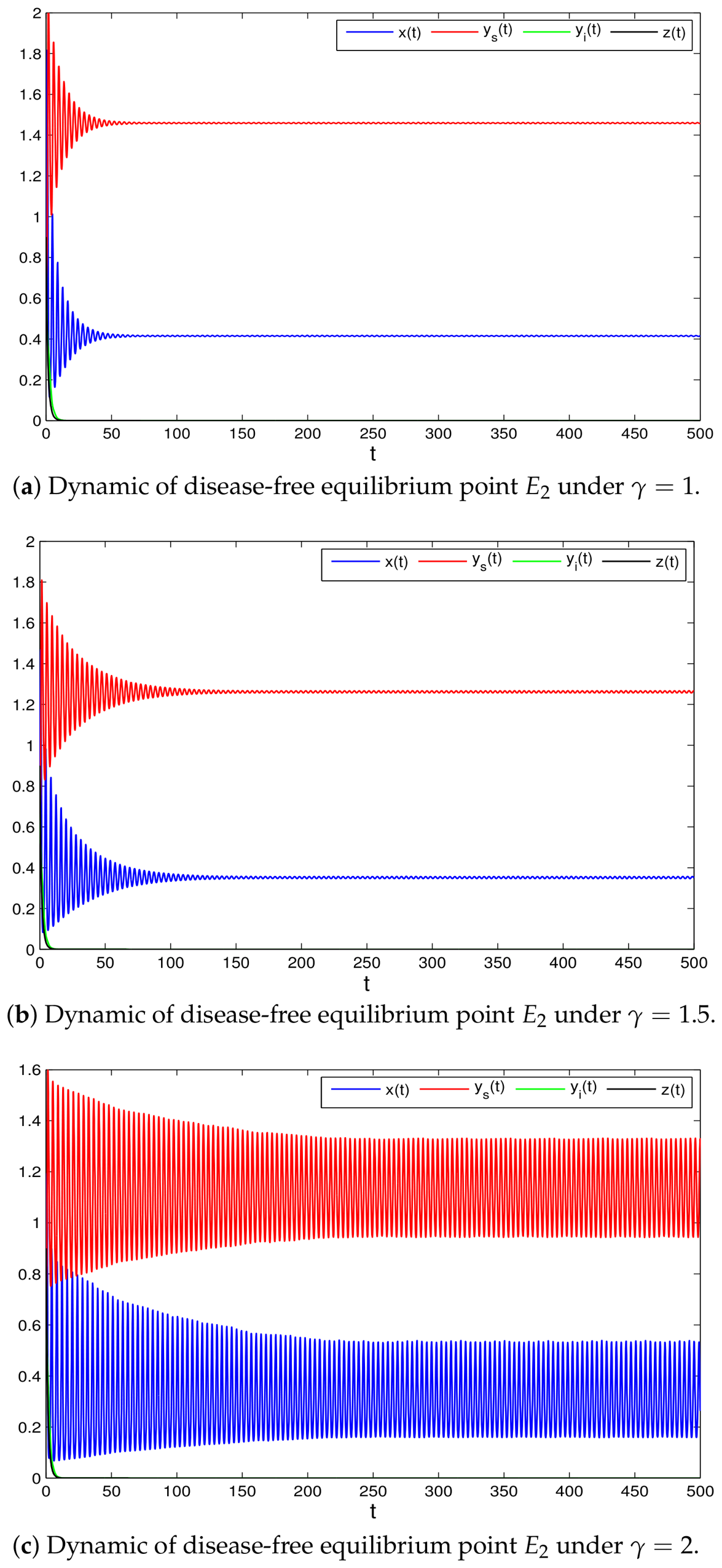
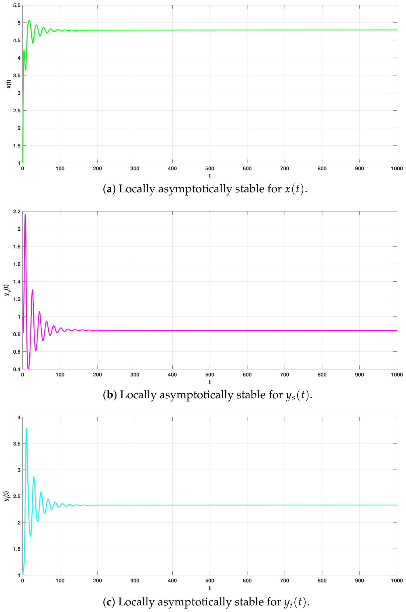
Numerous scholars have incorporated cooperative hunting into predation mechanisms to construct relevant predator–prey models and demonstrated that the cooperative hunting parameter is capable of inducing system bifurcation [19,20,21,22,23]. We further verify this conclusion via illustrative numerical examples. Setting $\varrho =1, r=4, k=3.5, \alpha =0.95,$$\eta =0.03, d=0.01, e=0.5, \theta =0.2, \mu =0.2, d_1=0.5, f=0.2, d_2=0.9, \phi =0.2, \epsilon =1.$ And by calculating that, we get $kd{e}^2{\alpha }^2+r{d}_1(1-ke\alpha )=-1.3171<0.$ Under such circumstances, system (5) admits the disease-free equilibrium $E_2$. Figure 1 shows that the stability of the disease-free equilibrium $E_2$ changes as $\gamma$ takes values of 1, $1.5$ and 2 under $\varrho =1$.

In Figure 1: (a) local asymptotic stability of the disease-free equilibrium $E_2$ holds at $\gamma =1$; (b) local asymptotic stability of the disease-free equilibrium $E_2$ holds at $\gamma =1.5$; (c) the disease-free equilibrium $E_2$ becomes unstable when $\gamma =2$.

Remark 2.

In Figure 1, we set $\varrho =1$, implying that the fractional-order system (5) reduces to the integer-order counterpart (4). With these parameters, the population of infected predators converges to zero, and the system degenerates into a classic predator–prey model with cooperative hunting.

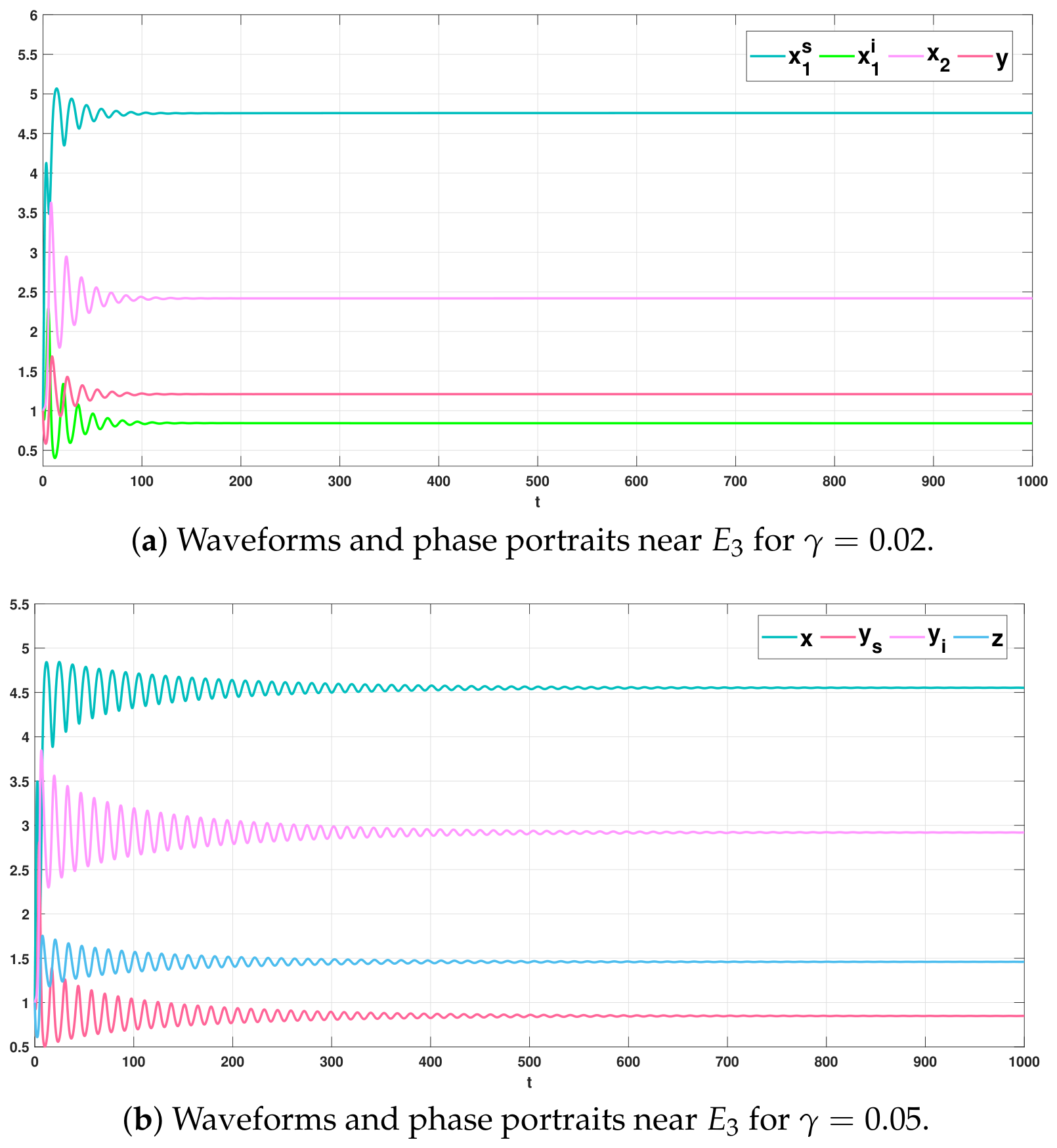
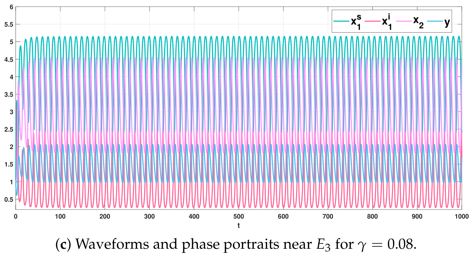
Below, we investigate how the cooperative hunting parameter affects the stability of fractional-order system (5). We fix the parameters as $r=1.6,k=6,\alpha =0.2,\gamma =\eta =0.02,d=0.1,e=0.8,\theta =\mu =0.2,d_1=0.05,f=0.5,d_2=0.3,\phi =0.5,\epsilon =1$. The coexistence equilibrium of system (5) is $E_3=(4.778,0.858,2.157,1.115)$. With fixed $\varrho =0.92$, we take three values of the cooperative hunting coefficient: $\gamma =0.02,0.05,0.08$. We examine the resulting time-series evolutions of system (5), as plotted in Figure 2. The results reveal that rising $\gamma$ gradually destabilizes the system. Accordingly, the cooperative hunting coefficient should be maintained within a proper range to preserve system stability.

Remark 3.

As the cooperative hunting parameter rises, susceptible predators gain substantially improved prey-capturing capability. With the prey population fixed, a high predation success rate drives a continuous decline in prey abundance. Infected predators possess restricted hunting efficiency. A marked drop in available prey further limits their food intake. Sustained depletion of prey in this manner inevitably destabilizes the whole ecosystem.

In Figure 2: (a) waveforms and phase portraits near $E_3$ for $\gamma =0.02$; (b) waveforms and phase portraits near $E_3$ for $\gamma =0.05$; (c) waveforms and phase portraits near $E_3$ for $\gamma =0.08$.

Example 2.

Hopf bifurcation induced by latency delay.

We next investigate the impacts of latency delay and fractional order on the stability of the coexistence equilibrium. The fixed parameters are specified as $r=1.6,k=6,\alpha =0.2,\gamma =0.005,\eta =0.02,d=0.1,e=0.8,\theta =\mu =0.2,d_1=0.05,f=0.5,d_2=0.3,\phi =0.5,\epsilon =1$.

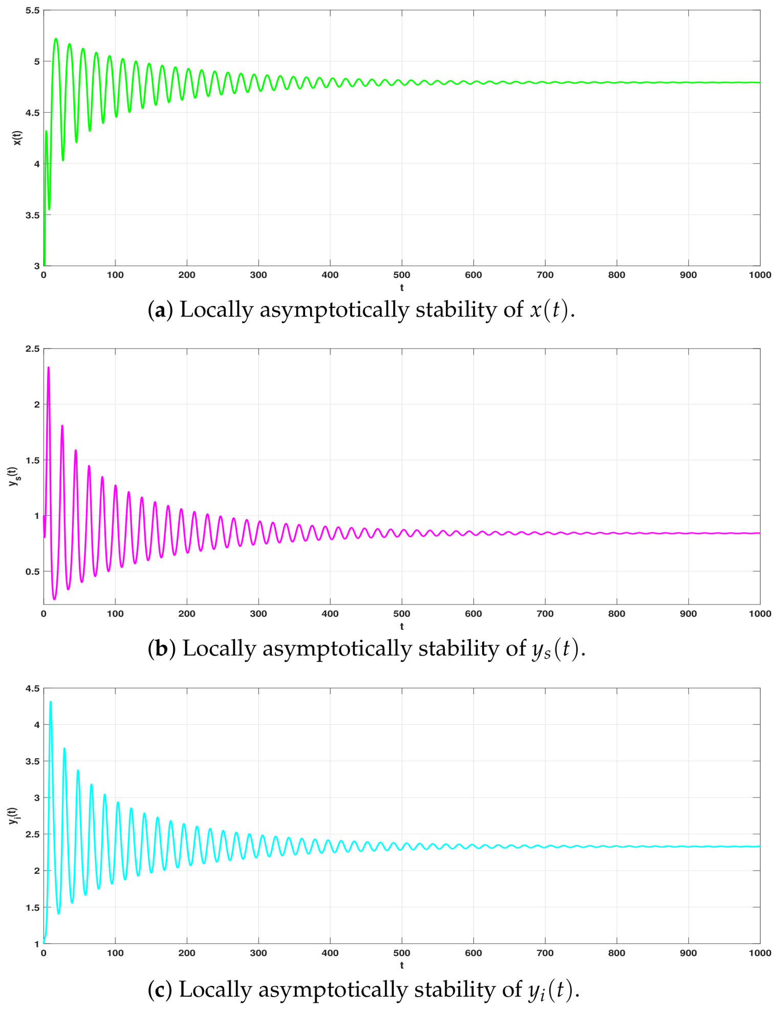
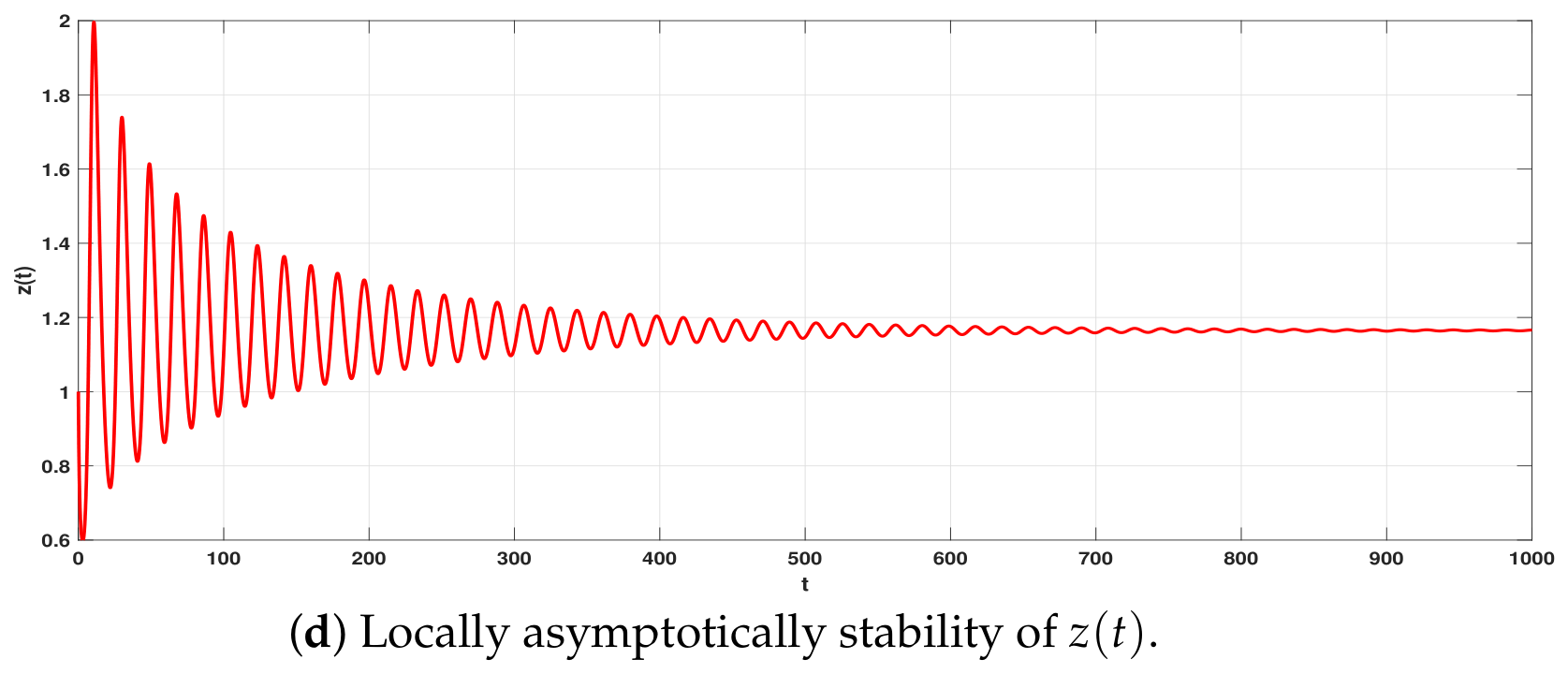
Under such a parameter configuration, the coexistence equilibrium reads $E_3=(4.783,0.857,2.332,1.162)$.

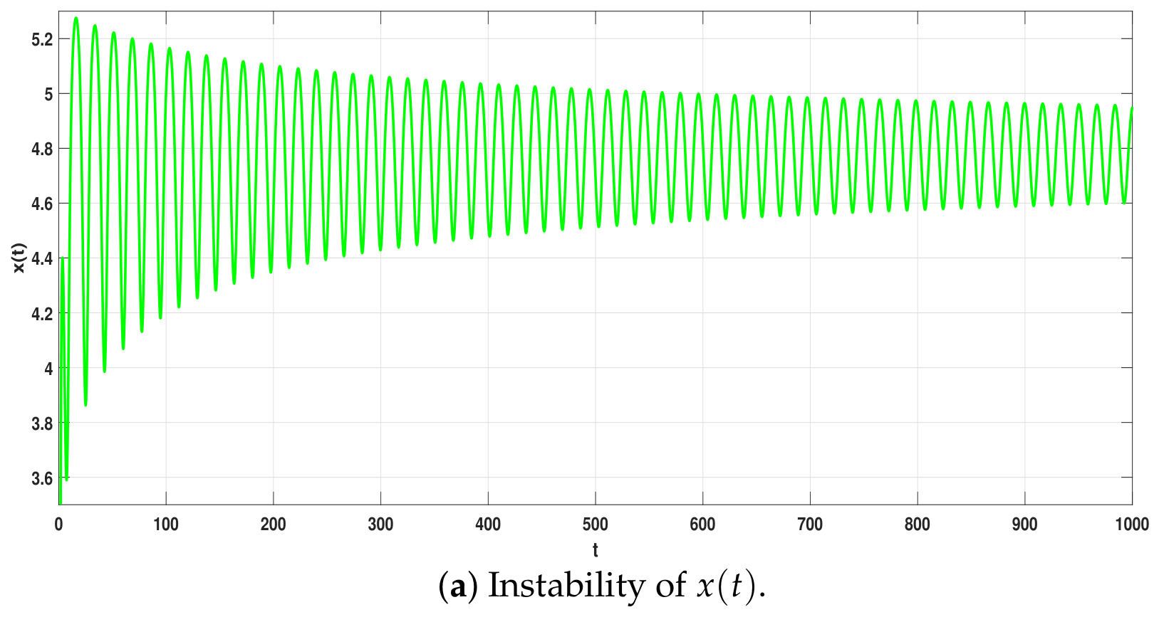
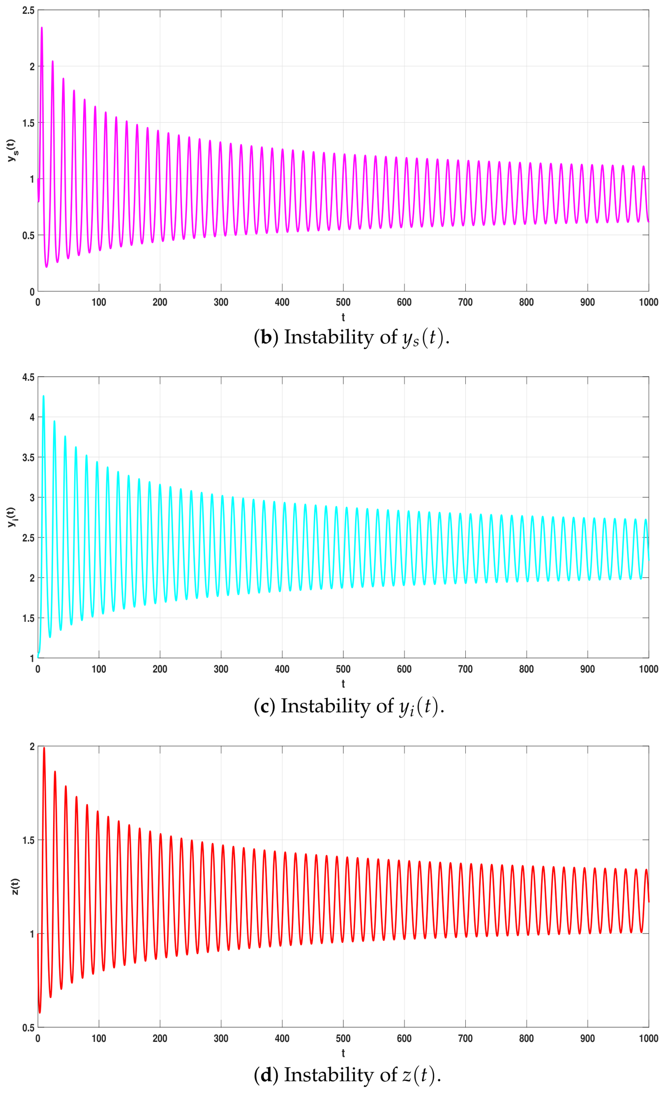
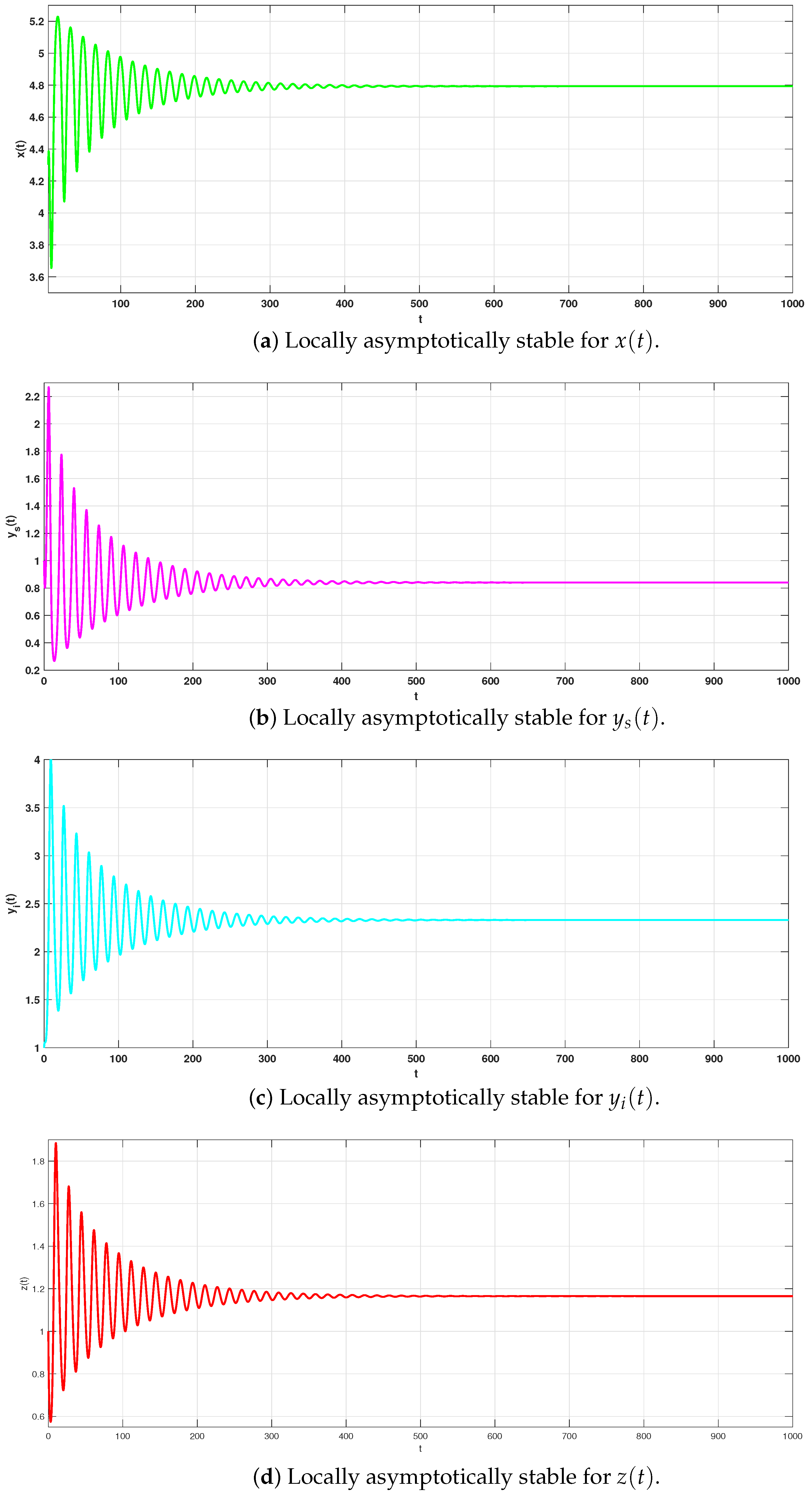
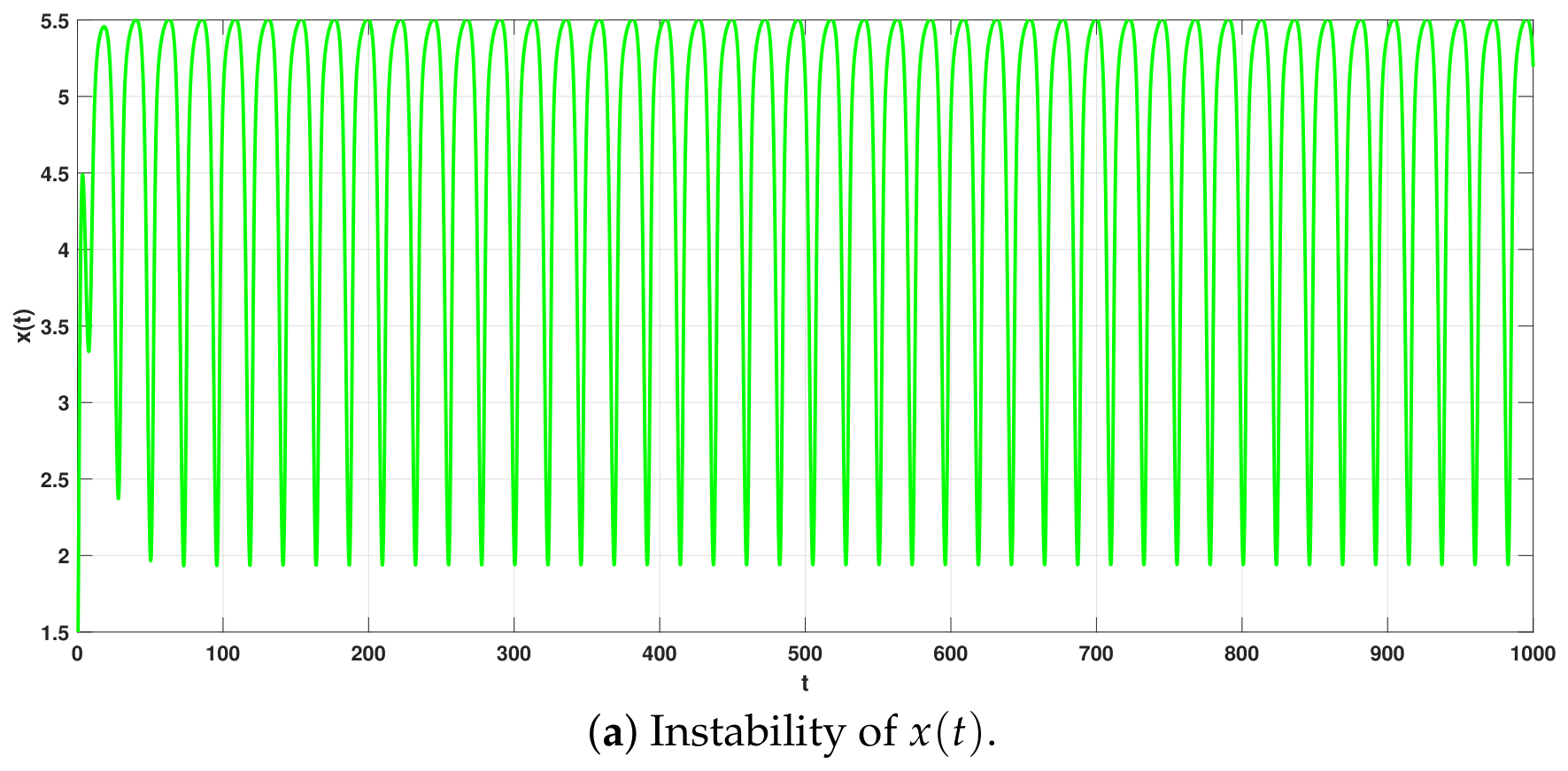
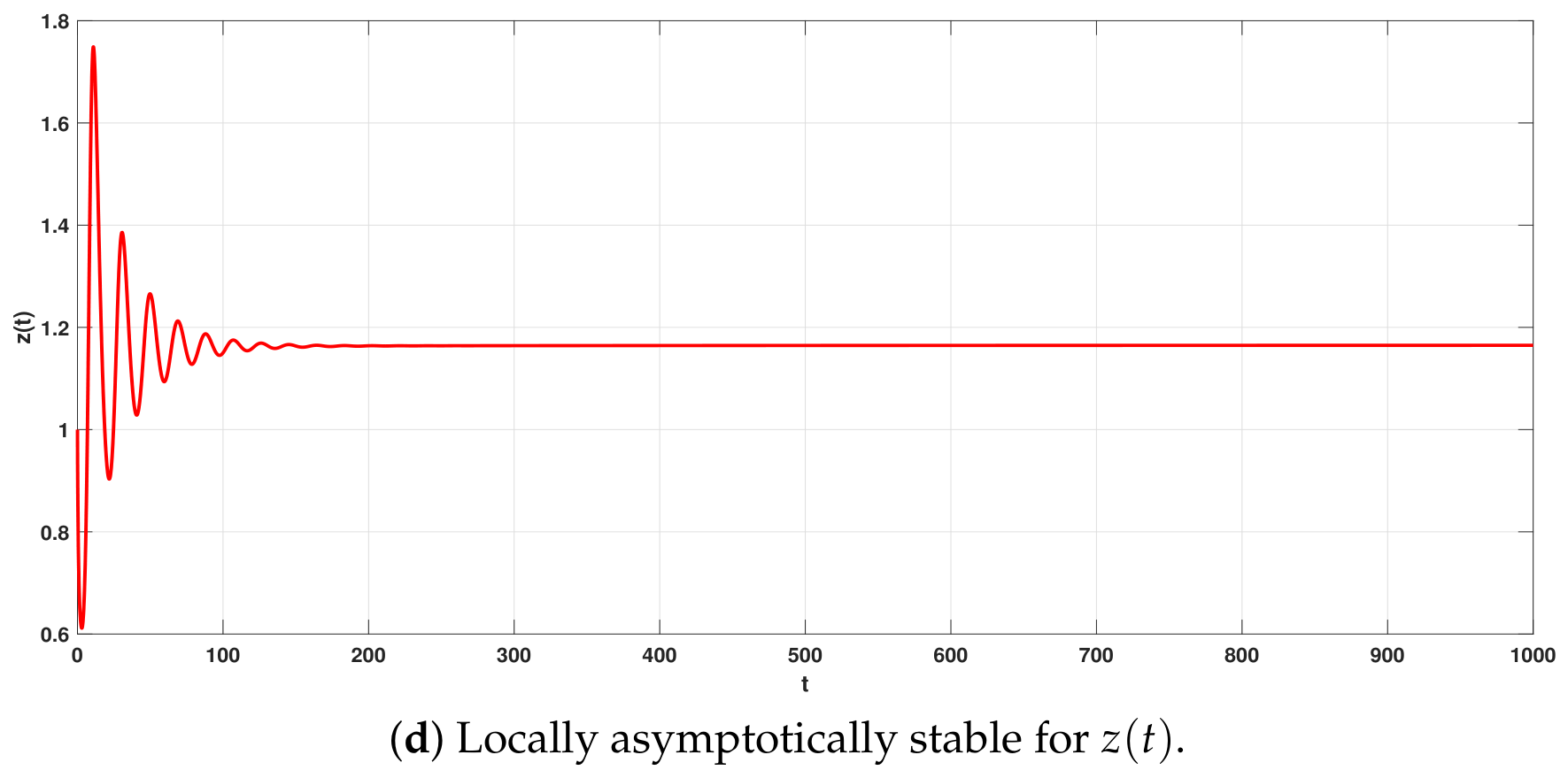
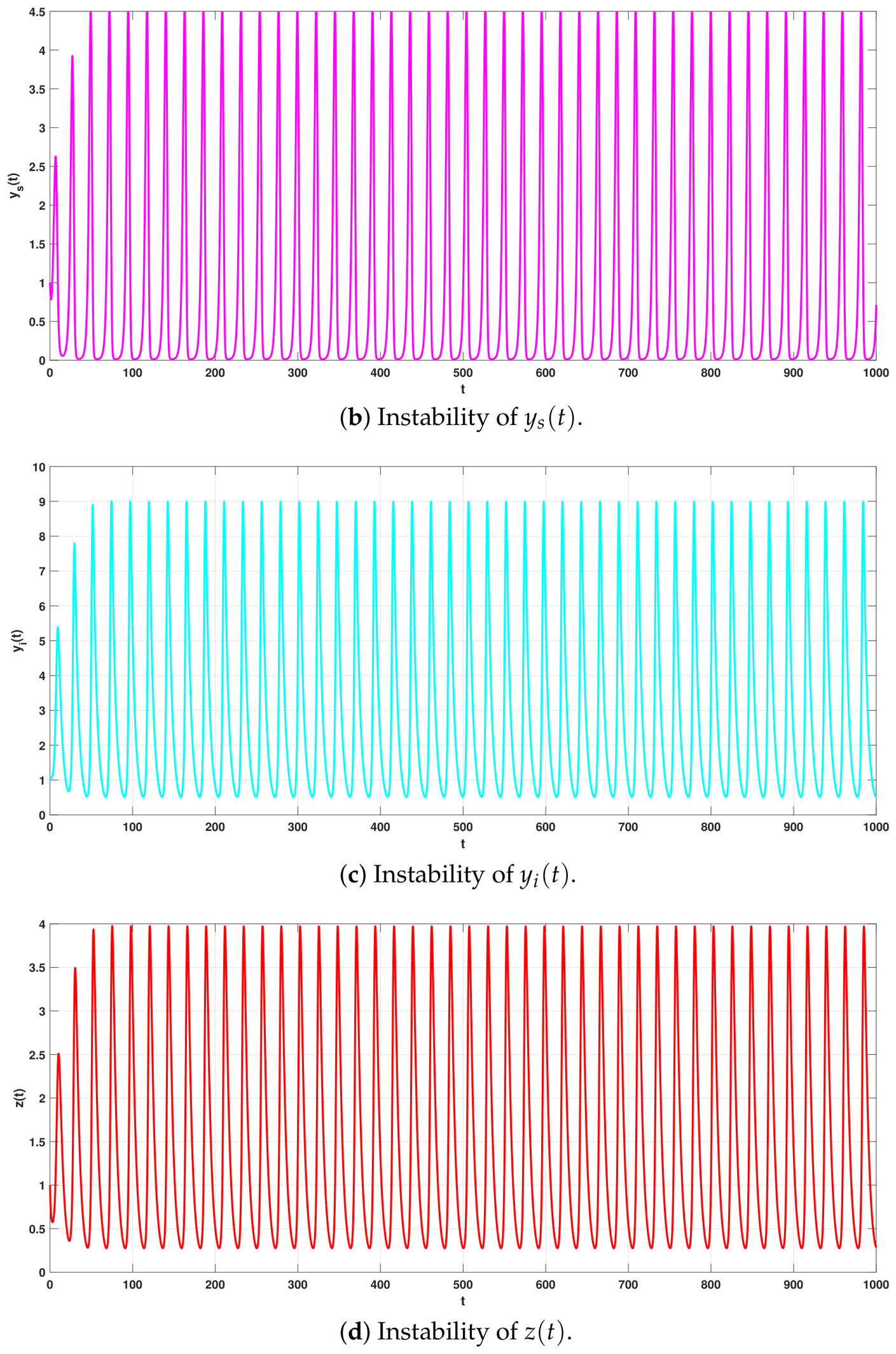
First, fix $\varrho =0.95$ to determine the critical bifurcation value ${\tau }_0$ for the onset of Hopf bifurcation. After verifying the transversality condition $H_3$ holds, theoretical calculations yield the bifurcation threshold ${\tau }_0=0.75$. We then adjust the latency delay: setting $\tau =0.8>{\tau }_0$, the corresponding numerical results are plotted in Figure 3. The resulting oscillatory time series and closed hollow orbits in the phase portrait demonstrate system instability. Next, we take $\tau =0.7<{\tau }_0$, with simulation outcomes presented in Figure 4. The system regains local stability at this smaller delay value.

In Figure 3: (a) waveforms and phase portraits near $E_3$ for $x(t)$; (b) waveforms and phase portraits near $E_3$ for $y_s(t)$; (c) waveforms and phase portraits near $E_3$ for $y_i(t)$; (d) waveforms and phase portraits near $E_3$ for $z(t)$.

In Figure 4: (a) waveforms and phase portraits near $E_3$ for $x(t)$; (b) waveforms and phase portraits near $E_3$ for $y_s(t)$; (c) waveforms and phase portraits near $E_3$ for $y_i(t)$; (d) waveforms and phase portraits near $E_3$ for $z(t)$.

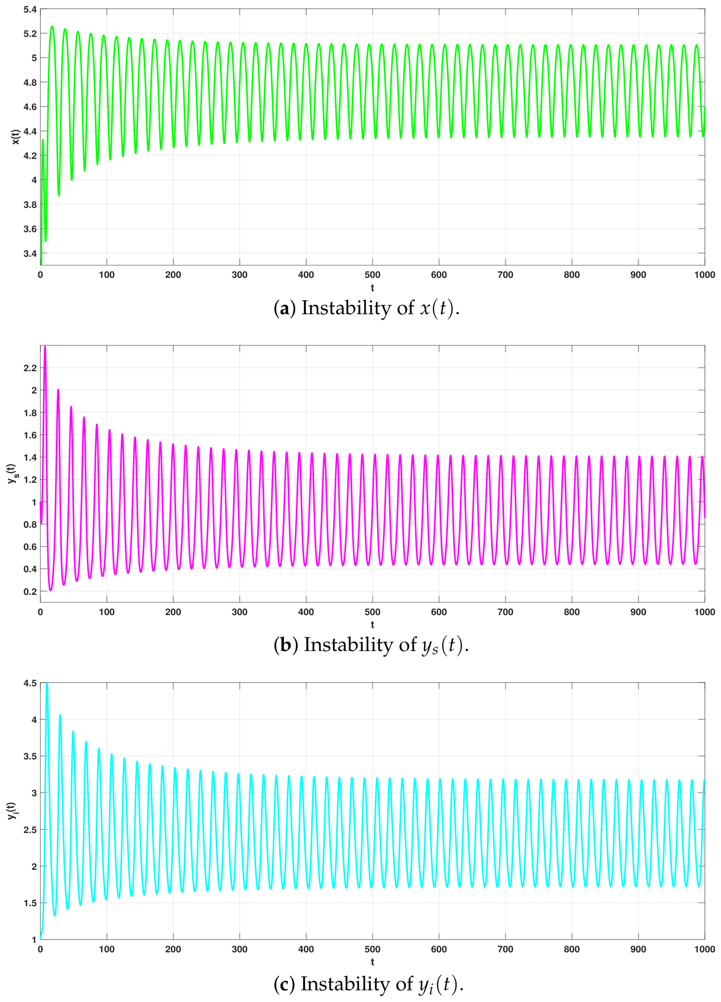
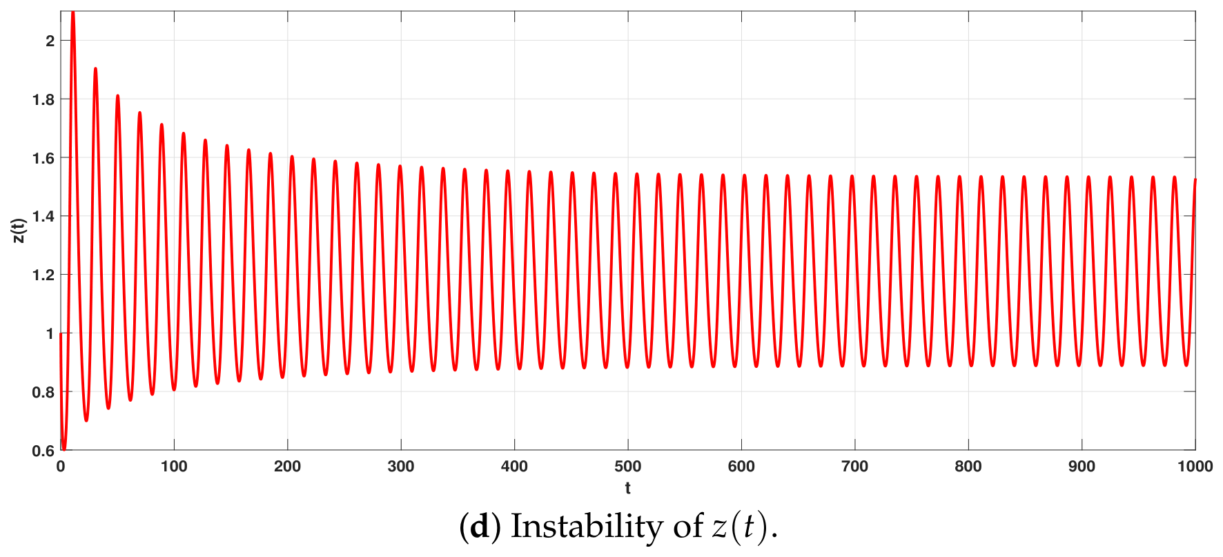
Theoretical analysis reveals that the bifurcation threshold depends on the fractional order. We next fix $\varrho =0.9$ and compute the critical bifurcation value ${\tau }^{\ast }=1.35$. When $\tau =1.5>{\tau }^{\ast }$, system (5) loses stability near $E_3$, as depicted in Figure 5. By contrast, setting $\tau =1.3<{\tau }^{\ast }$ renders the equilibrium $E_3$ locally asymptotically stable (see Figure 6). The stability shifts observed in Figure 3, Figure 4, Figure 5 and Figure 6 therefore validate Theorem 7.

In Figure 5: (a) waveforms and phase portraits near $E_3$ for $x(t)$; (b) waveforms and phase portraits near $E_3$ for $y_s(t)$; (c) waveforms and phase portraits near $E_3$ for $y_i(t)$; (d) waveforms and phase portraits near $E_3$ for $z(t)$.

In Figure 6: (a) waveforms and phase portraits near $E_3$ for $x(t)$; (b) waveforms and phase portraits near $E_3$ for $y_s(t)$; (c) waveforms and phase portraits near $E_3$ for $y_i(t)$; (d) waveforms and phase portraits near $E_3$ for $z(t)$.

Example 3.

Effects of fractional order on the system.

We examine how the fractional order affects the system’s stability domain, adopting all parameter values specified in Example 2.

We first exclude time delay to analyze the fractional-order impacts on the stability region of the delay-free system.

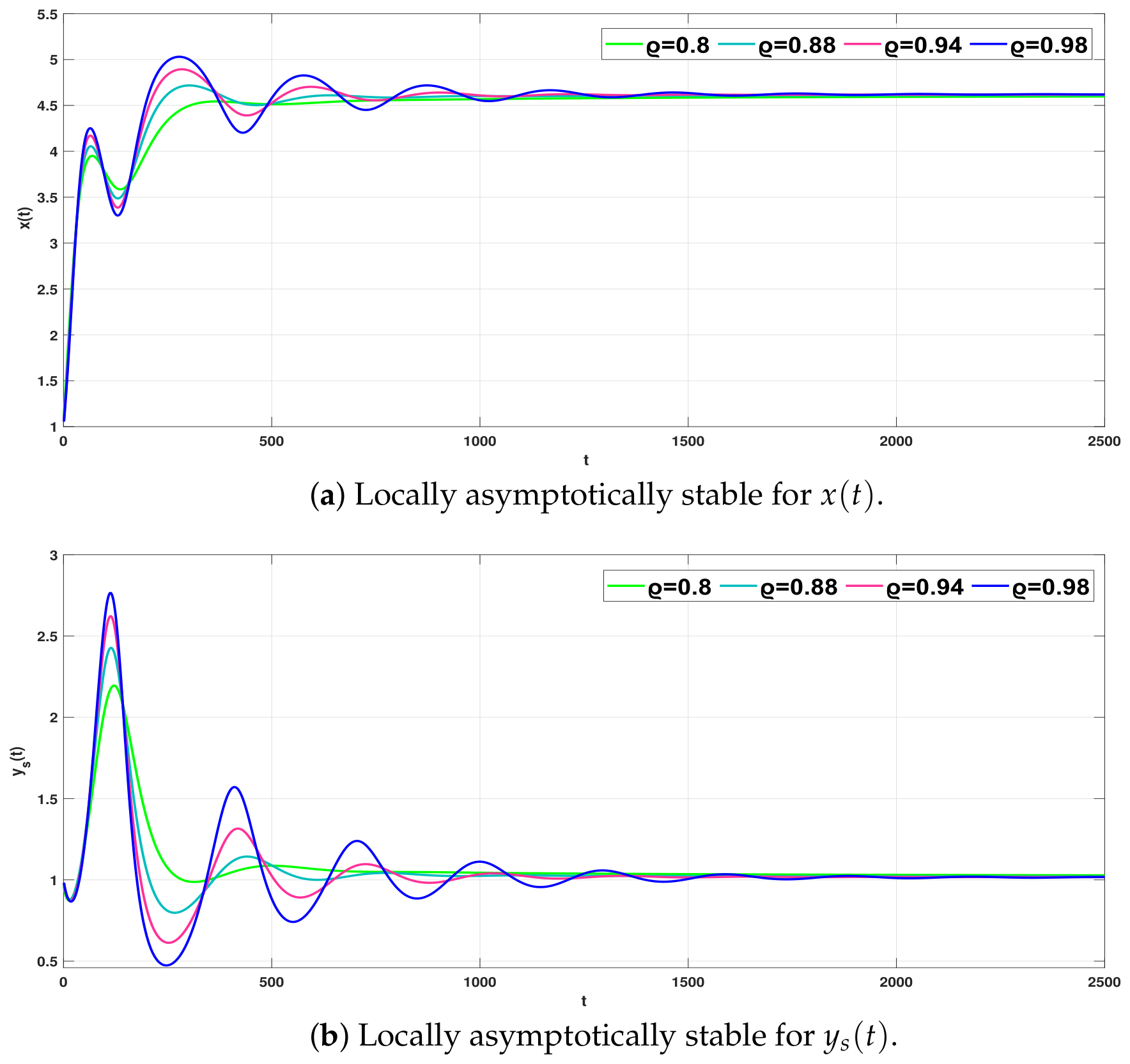
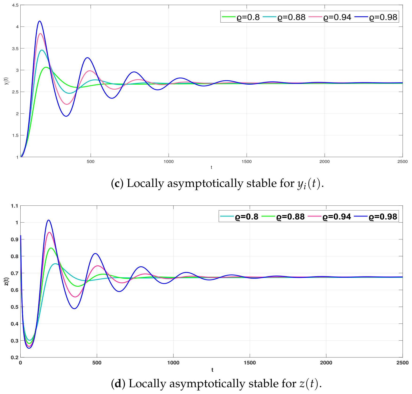
Four values $\varrho =0.8,0.88,0.94,0.98$ are chosen for comparison.

Figure 7 illustrates the trajectories of all state variables in system (5) across distinct $\varrho$.

Numerical results indicate that decreasing the fractional order accelerates the system’s convergence to a stable steady state.

Next, we fix $\tau =1.3$ and vary $\varrho$.

Figure 8 presents time trajectories and phase portraits of system (5) near coexistence equilibrium $E_3$ for $\varrho =0.98$, revealing system instability. This outcome contrasts sharply with Figure 6 and implies the critical bifurcation threshold is smaller than $1.35$.

In Figure 7: (a) waveforms and phase portraits near $E_3$ for $x(t)$; (b) waveforms and phase portraits near $E_3$ for $y_s(t)$; (c) waveforms and phase portraits near $E_3$ for $y_i(t)$; (d) waveforms and phase portraits near $E_3$ for $z(t)$.

In Figure 8: (a) waveforms and phase portraits near $E_3$ for $x(t)$; (b) waveforms and phase portraits near $E_3$ for $y_s(t)$; (c) waveforms and phase portraits near $E_3$ for $y_i(t)$; (d) waveforms and phase portraits near $E_3$ for $z(t)$.

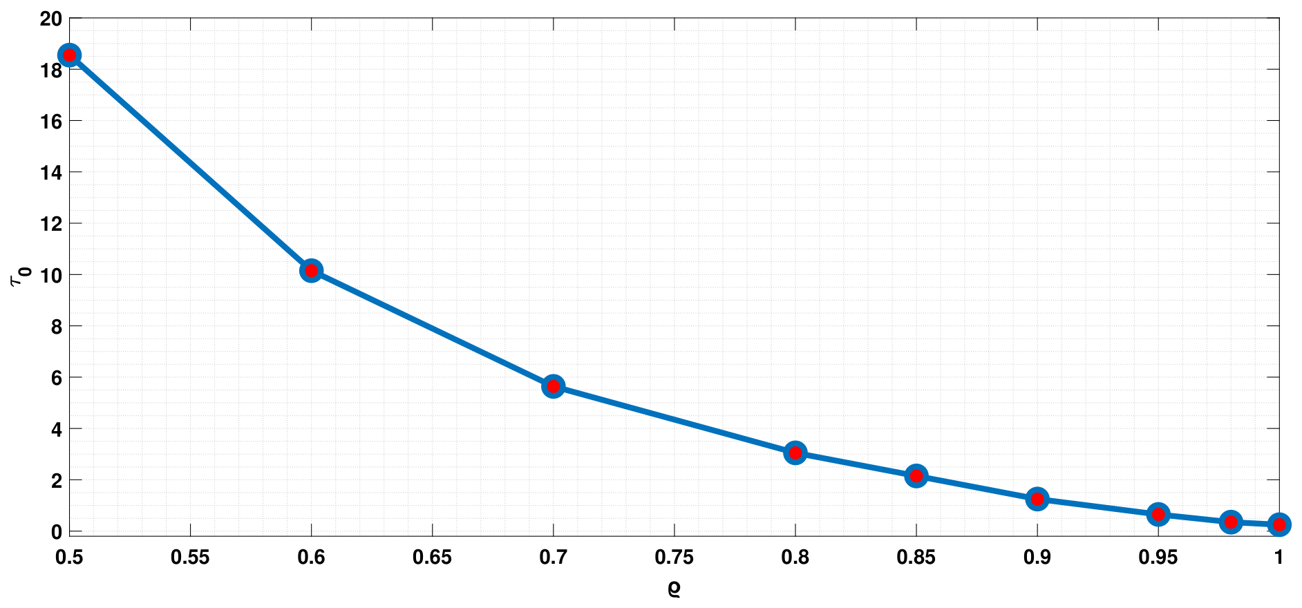
With fixed $\tau =1.3$ and $\varrho =0.85$, Figure 9 displays time trajectories and phase portraits of system (5) around $E_3$, where the equilibrium is asymptotically stable. Compared with Figure 6, the time series in Figure 9 converges faster with markedly weaker oscillation amplitudes, which suggests the corresponding bifurcation threshold exceeds $1.35$. Results from Figure 8 and Figure 9 demonstrate the fractional-order parameter’s impact on the critical bifurcation value: a smaller fractional order yields a larger threshold ${\tau }_0$ and hence postpones the onset of Hopf bifurcation. Figure 10 further intuitively characterizes the quantitative relation between $\varrho$ and ${\tau }_0$.

In Figure 9: (a) waveforms and phase portraits near $E_3$ for $x(t)$; (b) waveforms and phase portraits near $E_3$ for $y_s(t)$; (c) waveforms and phase portraits near $E_3$ for $y_i(t)$; (d) waveforms and phase portraits near $E_3$ for $z(t)$.

Remark 4.

The derived theoretical results can be interpreted ecologically from three key parameters: cooperative hunting strength, disease latency delay, and fractional order. First, excessive cooperative hunting destabilizes coexisting populations: intensified group predation depletes prey resources rapidly, creating food scarcity for diseased solitary predators and triggering cyclic population oscillations. Second, latency delay drives Hopf bifurcation: a short latent period ($\tau <{\tau }_0$) restricts pathogen transmission and stabilizes the ecosystem, while overly prolonged latency ($\tau >{\tau }_0$) lets asymptomatic infected predators continuously contaminate the environment, sparking recurrent epidemic fluctuations. Third, the fractional order describes ecosystem historical memory. A smaller fractional order strengthens memory effects, accelerating the system’s convergence to steady state and raising the critical bifurcation threshold ${\tau }_0$, which improves the ecosystem’s resistance to disease-induced periodic outbreaks. Collectively, these findings provide ecological suggestions for wildlife management: controlling predator cooperative intensity and shortening pathogen latent duration effectively maintain population stability.

7. Conclusions

A novel fractal-order model of predator–prey systems is proposed that combines the characteristics of cooperative hunting and environmental infection, with a particular focus on the spread of disease between predator populations. As opposed to the traditional model, this study not only considers the direct mode of disease transmission but also introduces the mechanism of environmental transmission. This innovative perspective, which is the first of its type in eco-epidemiological research, allows us to better understand how pathogens affect predator population dynamics in natural environments. In the case of a group of social predators that have long practiced cooperative hunting strategies, the study finds that the spread of disease can seriously disrupt this cooperative relationship, thereby affecting the survival and reproduction of the population. We study the solution of the system in depth and obtain results for the boundedness, existence of the equilibrium point, and local asymptotic stability of the system. Our results provide a theoretical foundation for understanding predator population dynamics. Furthermore, we introduce the latency delay of the disease as a bifurcation parameter and obtain the sufficient conditions for Hopf bifurcation. This finding shows that when the latency delay exceeds a certain critical value ${\tau }_0$, Hopf bifurcation occurs in the system, resulting in fundamental changes in the dynamic behavior of the ecosystem. The numerical simulation results further verify our theoretical analysis conclusion: when $\tau =0$, the coexistence equilibrium points in the system show asymptotic stability, and when $\tau <{\tau }_0$, the system can maintain a stable state. However, when $\tau >{\tau }_0$, the stability of the system is destroyed, causing the balance between predators and prey to break down. Moreover, different fractional exponents lead to different stable convergence rates, which can be explained by the long-term memory effect embodied by the fractional derivatives. This memory feature is important in ecological models because it reflects the complex dynamic interactions between predators and prey, thereby providing insights into the evolution of ecosystems. Through numerical examples, it is found that the reduction in the fractional order number prolongs the Hopf bifurcation time.

In addition, biologically, our infection model is simplified to ease stability and bifurcation analysis, omitting multi-stage disease progression, graded infection severity, and infected predator heterogeneity, which reduces biological realism. For future work, we will subdivide infected predators into exposed, mild, and severe compartments and adopt heterogeneous infection parameters. Our core analytical methods (Jacobian stability, Mittag-Leffler boundedness, Hopf bifurcation) can be extended to these refined, more realistic models.

References

1. Shi, L.; Zhou, J.; Ye, Y. Global stability and Hopf bifurcation ofnetworked respiratory disease model with delay. Appl. Math. Lett. 2024, 151, 109000. [Google Scholar]
2. Jia, L.; Tan, H.; Cao, H. Analysis of Dynamics of a Recurrent Infectious Disease SIRS Model with Age Structure and Two Delays. Int. J. Bifurc. Chaos 2024, 34, 2450128. [Google Scholar] [CrossRef]
3. Ghaziani, R.K.; Govaerts, W.; Sonck, C. Resonance and bifurcation in a discrete-time predator-prey system with Holling functional response. Nonlinear Anal. Real. World Appl. 2012, 13, 1451–1465. [Google Scholar]
4. Rosen, L. The natural history of Japanese encephalitis virus. Annu. Rev. Microbiol. 1986, 40, 395–414. [Google Scholar] [CrossRef] [PubMed]
5. Iboi, E.; Okuonghae, D. Population dynamics of a mathematical model for syphilis. Appl. Math. Model. 2016, 40, 3573–3590. [Google Scholar] [CrossRef]
6. Alharbi, R.; Jan, R.; Alyobi, S.; Altayeb, Y.; Khan, Z. Mathematical modeling and stability analysis of the dynamics of monkeypox via fractional-calculus. Fractals 2022, 30, 2240266. [Google Scholar] [CrossRef]
7. Wang, L.F.; Crameri, G. Emerging zoonotic viral diseases. Rev. Sci. Tech 2014, 33, 569–581. [Google Scholar] [CrossRef] [PubMed]
8. Rahman, M.T.; Sobur, M.A.; Islam, M.S.; Ievy, S.; Hossain, M.J.; El Zowalaty, M.E.; Rahman, A.T.; Ashour, H.M. Zoonotic diseases: Etiology, impact, and control. Microorganisms 2020, 8, 1405. [Google Scholar] [CrossRef] [PubMed]
9. Liu, X.; Liu, S. Dynamics of a predator-prey system with inducible defense and disease in the prey. Nonlinear Anal. Real. World Appl. 2023, 71, 103802. [Google Scholar]
10. Thirthar, A.A.; Sk, N.; Mondal, B.; Alqudah, M.A.; Abdeljawad, T. Utilizing memory effects to enhance resilience in disease-driven prey-predator systems under the influence of global warming. J. Appl. Math. Comput. 2023, 69, 4617–4643. [Google Scholar]
11. Ghanbari, B. A new model for investigating the transmission of infectious diseases in a prey-predator system using a non-singular fractional derivative. Math. Methods Appl. Sci. 2023, 46, 8106–8125. [Google Scholar]
12. Gashirai, T.B.; Musekwa-Hove, S.D.; Lolika, P.O.; Mushayabasa, S. Global stability and optimal control analysis of a foot-and-mouth disease model with vaccine failure and environmental transmission. Chaos Solitons Fractals 2020, 132, 109568. [Google Scholar]
13. Geng, Y.; Wang, Y. Stability and transmissibility of SARS-CoV-2 in the environment. J. Med. Virol. 2023, 95, e28103. [Google Scholar] [PubMed]
14. Li, J.; Jia, K.; Zhao, W.; Yuan, B.; Liu, Y. Natural and socio-environmental factors contribute to the transmissibility of COVID-19: Evidence from an improved SEIR model. Int. J. Biometeorol. 2023, 67, 1789–1802. [Google Scholar] [CrossRef] [PubMed]
15. Breban, R.; Drake, J.M.; Stallknecht, D.E.; Rohani, P. The role of environmental transmission in recurrent avian influenza epidemics. PLoS Comput. Biol. 2009, 5, e1000346. [Google Scholar] [CrossRef] [PubMed]
16. Islam, W.; Noman, A.; Naveed, H.; Alamri, S.A.; Hashem, M.; Huang, Z.; Chen, H.Y.H. Plant-insect vector-virus interactions under environmental change. Sci. Total Environ. 2020, 701, 135044. [Google Scholar] [PubMed]
17. Foley, J.; Clifford, D.; Castle, K.; Cryan, P.; Ostfeld, R.S. Investigating and managing the rapid emergence of white-nose syndrome, a novel, fatal, infectious disease of hibernating bats. Conserv. Biol. 2011, 25, 223–231. [Google Scholar] [PubMed]
18. Wilder, A.P.; Kunz, T.H.; Sorenson, M.D. Population genetic structure of a common host predicts the spread of white-nose syndrome, an emerging infectious disease in bats. Mol. Ecol. 2015, 24, 5495–5506. [Google Scholar] [PubMed]
19. Pal, S.; Pal, N.; Samanta, S.; Chattopadhyay, J. Effect of hunting cooperation and fear in a predator-prey model. Ecol. Complex. 2019, 39, 100770. [Google Scholar] [CrossRef]
20. Dey, S.; Banerjee, M.; Ghorai, S. Bifurcation analysis and spatio-temporal patterns of a prey-predator model with hunting cooperation. Int. J. Bifurc. Chaos 2022, 32, 2250173. [Google Scholar]
21. Shivam; Singh, K.; Kumar, M.; Dubey, R.; Singh, T. Untangling role of cooperative hunting among predators and herd behavior in prey with a dynamical systems approach. Chaos Solitons Fractals 2022, 162, 112420. [Google Scholar] [CrossRef]
22. Saha, S.; Samanta, G.P. A prey-predator system with disease in prey and cooperative hunting strategy in predator. J. Phys. A Math. Theor. 2020, 53, 485601. [Google Scholar]
23. Liu, J.; Liu, B.; Lv, P.; Zhang, T. An eco-epidemiological model with fear effect and hunting cooperation. Chaos Solitons Fractals 2021, 142, 110494. [Google Scholar] [CrossRef]
24. Loehle, C. Social barriers to pathogen transmission in wild animal populations. Ecology 1995, 76, 326–335. [Google Scholar] [CrossRef]
25. Li, C.; Deng, W. Remarks on fractional derivatives. Appl. Math. Comput. 2007, 187, 777–784. [Google Scholar] [CrossRef]
26. Podlubny, I. An Introduction to Fractional Derivatives, Fractional Differential Equations, to Methods of Their Solution and Some of Their Applications. In Fractional Differential Equations; Elsevier: Amsterdam, The Netherlands, 1998. [Google Scholar]
27. Jin, B. Fractional Differential Equations: An Approach via Fractional Derivatives; Springer: Cham, Switzerland, 2021; Volume 206. [Google Scholar]
28. Kumar, A.; Kumar, S. A study on eco-epidemiological modelwith fractional operators. Chaos Solitons Fractals 2022, 156, 111697. [Google Scholar]
29. Mahata, A.; Paul, S.; Mukherjee, S.; Das, M.; Roy, B. Dynamics of caputofractional order SEIRV epidemic model with optimal controland stability analysis. Int. J. Appl. Comput. Math. 2022, 8, 28. [Google Scholar] [PubMed]
30. Rihan, F.A.; Rajivganthi, C. Dynamics of fractional-order delaydifferential model of prey-predator system with Holling-type and infection among predators. Chaos Solitons Fractals 2020, 141, 110365. [Google Scholar]
31. Yaagoub, Z.; Danane, J.; Hammouch, Z.; Allali, K. Mathematicalanalysis of a fractional order two strain SElR epidemic model. Results Nonlinear Anal. 2024, 7, 156–175. [Google Scholar]
32. Li, N.; Yan, M. Bifurcation control of a delayed fractional-order predator-prey model with cannibalism and disease. Phys. A Stat. Mech. Its Appl. 2022, 600, 127600. [Google Scholar]
33. Zhang, H.; Muhammadhaji, A. Dynamics of a Delayed Fractional-Order Predator-prey Model with Cannibalism and Disease in Prey. Fractal Fract. 2024, 8, 333. [Google Scholar]
34. Du, W.; Xiao, M.; Ding, J.; Yao, Y.; Wang, Z.; Yang, X. Fractional-order PD control at Hopf bifurcation in a delayed predator-prey system with trans-species infectious diseases. Math. Comput. Simul. 2023, 205, 414–438. [Google Scholar]
35. Singh, H. Numerical simulation for fractional delay differential equations. Int. J. Dyn. Control 2021, 9, 463–474. [Google Scholar]
36. Kaslik, E.; Sivasundaram, S. Analytical and numerical methods for the stability analysis of linear fractional delay differential equations. J. Comput. Appl. Math. 2012, 236, 4027–4041. [Google Scholar] [CrossRef]
37. Zeng, J.; Chen, X.; Wei, L.; Li, D. Bifurcation analysis of afractional-order eco-epidemiological system with two delays. Nonlinear Dyn. 2024, 112, 22505–22527. [Google Scholar]
38. Wang, X.; Wang, Z.; Xia, J. Stability and bifurcation control of adelayed fractional-order eco-epidemiological model withincommensurate orders. J. Frankl. Inst. 2019, 356, 8278–8295. [Google Scholar]
39. Uddin, M.J.; Podder, C.N. Fractional order prey-predator model incorporating immigration on prey: Complexity analysis and itscontrol. Int. J. Biomath. 2024, 17, 2350051. [Google Scholar]
40. Song, C.; Li, N. Dynamic analysis and bifurcation control of a delayed fractional-order eco-epidemiological migratory bird model with fear effect. Int. J. Biomath. 2024, 17, 2350022. [Google Scholar]
41. Hilker, F.M.; Paliga, M.; Venturino, E. Diseased social predators. Bull. Math. Biol. 2017, 79, 2175–2196. [Google Scholar] [CrossRef] [PubMed]
42. Petráš, I. Fractional-Order Nonlinear Systems: Modeling, Analysis and Simulation; Higher Education Press: Beijing, China, 2011. [Google Scholar]
43. Li, H.L.; Zhang, L.; Hu, C.; Jiang, Y.-L.; Teng, Z. Dynamical analysis of a fractional-order predator-prey model incorporating a prey refuge. J. Appl. Math. Comput. 2017, 54, 435–449. [Google Scholar]
44. Bhalekar, S.; Daftardar-Gejji, V. A predictor-corrector scheme for solving nonlinear delay differential equations of fractional order. Fract. Calc. Appl. Anal. 2011, 1, 1–9. [Google Scholar]
45. Diethelm, K.; Ford, N.J.; Freed, A.D. Detailed error analysis for a fractional Adams method. Numer. Algorithms 2004, 36, 31–52. [Google Scholar] [CrossRef]
Figure 1. Dynamic behavior of disease-free equilibrium point E 2 under different γ .
Appliedmath 06 00108 g001
Figure 2. Waveforms and phase portraits near E 3 for different γ ( ϱ = 0.92 ).
Appliedmath 06 00108 g002aAppliedmath 06 00108 g002b
Figure 3. Waveform plots and phase portraits of system (5) when ϱ = 0.95 , τ = 0.8 > τ 0 = 0.75 .
Appliedmath 06 00108 g003aAppliedmath 06 00108 g003b
Figure 4. Waveform plots and phase portraits of system (5) when ϱ = 0.95 , τ = 0.7 < τ 0 = 0.75 .
Appliedmath 06 00108 g004
Figure 5. Waveform plots and phase portraits of system (5) when ϱ = 0.9 , τ = 1.5 > τ 0 = 1.35 .
Appliedmath 06 00108 g005aAppliedmath 06 00108 g005b
Figure 6. Waveform plots and phase portraits of system (5) when ϱ = 0.9 , τ = 1.3 < τ 0 = 1.35 .
Appliedmath 06 00108 g006aAppliedmath 06 00108 g006b
Figure 7. Waveform plots of system (5) when ϱ = 0.8 , 0.88 , 0.94 , 0.98 .
Appliedmath 06 00108 g007aAppliedmath 06 00108 g007b
Figure 8. Waveform plots and phase portraits of system (5) when ϱ = 0.98 , τ = 1.3 .
Appliedmath 06 00108 g008aAppliedmath 06 00108 g008b
Figure 9. Waveform plots and phase portraits of system (5) when ϱ = 0.85 , τ = 1.3 .
Appliedmath 06 00108 g009aAppliedmath 06 00108 g009b
Figure 10. Influence of fractional Order ϱ on bifurcation threshold τ 0 .
Appliedmath 06 00108 g010