Interpolative Geraghty-Type Contractions in Bicomplex-Valued Metric Spaces: Fixed Point Results, Stability Analysis, and Applications

Abstract

In this paper, we introduce and systematically study the class of interpolative Geraghty-type contractive mappings within the framework of complete bicomplex-valued metric spaces (bi-CVMS). We prove seven new results: (i) a fixed point theorem for a single interpolative Geraghty contraction; (ii) a common fixed point theorem for a pair of such mappings; (iii) a fixed point theorem for interpolative Reich–Rus–Ćirić type contractions in bi-CVMS; (iv) a coincidence point and common fixed point theorem for weakly compatible maps; (v) a fixed point theorem for Jaggi-type hybrid contractions in bi-CVMS; (vi) a stability result for the Picard iteration associated with the main contraction; and (vii) an application theorem establishing the existence and uniqueness of solutions to a boundary value problem governed by a Caputo fractional differential equation. All results are furnished with complete proofs and non-trivial illustrative examples. Several well-known theorems—including those of Banach, Kannan, Reich, Geraghty, and their complex-valued analogues—follow as special cases. The paper significantly advances the fixed point theory in bicomplex-valued metric spaces.

1. Introduction

The Banach contraction principle [1], asserting the existence and uniqueness of fixed points of strict contractions on complete metric spaces, remains after more than a century the most cited result in nonlinear analysis and provides the analytic foundation for iterative methods in differential equations, operator theory, and optimisation. Its generalisations proceed along two principal axes: (a) enrichment of the underlying space, and (b) weakening of the contraction condition. The present article advances both axes simultaneously within the framework of bicomplex-valued metric spaces. The bicomplex-valued metric space (bi-CVMS) offers three structural advantages over classical real or complex-valued metric spaces: (i) its metric takes values in ℂ₂, a commutative ring equipped with a natural partial order ≾ derived from the idempotent representation, enabling simultaneous tracking of two independent complex distance components; (ii) the idempotent decomposition ξ = β₁e₁ + β₂e₂ allows componentwise analysis, making it possible to reduce fixed point problems in bi-CVMS to pairs of problems in ℂ₁, which simplifies verification of contraction conditions in applications (see Section 9); and (iii) the bicomplex framework strictly contains the complex-valued setting of Azam et al. [2] as a special case (by taking i₁ = j), thus every result proved in bi-CVMS automatically yields a corresponding complex-valued result.

Regarding axis (a), Azam, Fisher, and Khan [2] introduced complex-valued metric spaces (CVMS) in 2011 as a specialisation of cone metric spaces admitting rational contractive inequalities. Their framework was extended to the bicomplex setting by Choi, Datta, Biswas, and Islam [3] in 2017, who proved common fixed point theorems for weakly compatible pairs in bicomplex-valued metric spaces (bi-CVMS). Subsequent contributions include rational contractions by Jebril, Datta, Sarkar and Biswas [4]; extrapolation fixed points by Beg, Datta and Pal [5]; bicomplex partial metric spaces and nonlinear integral equations by Gnanaprakasam, Boulaaras, Mani, Cherif and Idris [6]; linear equation systems by the same group [7]; point-dependent control functions by Abdou [8]; Fredholm integral equations by Mani, Gnanaprakasam et al. [9]; mixed rational contractions in bicomplex b-metric spaces by Arul Joseph et al. [10]; common fixed points with control functions of two variables by Tassaddiq et al. [11]; controlled metric space extensions by Gnanaprakasam et al. [12]; and generalised rational conditions with Volterra integral equation applications by Noman and Abdou [13].

Regarding axis (b), Geraghty [14] in 1973 replaced the Lipschitz constant by a function β belonging to the class $𝒮$:= {β: [0,∞) → [0,1): β(t_n) → 1 ⟹ t_n → 0}, obtaining a contraction principle that encompasses a rich family of mappings. Karapinar [15] introduced interpolative contractions in 2018 by distributing the contraction requirement across multiple distance components with fractional exponents summing to one. Interpolative Kannan [15], Reich–Rus–Ćirić [16], and Hardy–Rogers [17] contractions have since been established in various metric settings. A Jaggi-type hybrid interpolative contraction was studied by Karapinar, Agarwal, and Aydi [18]. The combination of interpolative contractions with Geraghty-type functions in the bicomplex framework has, to our knowledge, not yet been investigated. This gap motivates our work.

More recently, Wardowski-type F-contractions in bicomplex-valued metric spaces have been studied by Piri and Kumam [19] in the scalar setting, with analogous results in bi-CVMS being developed alongside controlled metric space generalisations. These post-2020 developments underscore the continuing vitality of fixed point theory in bicomplex frameworks.

Fixed point theory has developed as a fundamental area in nonlinear analysis with wide applications in differential equations, integral equations, and applied sciences. Classical contributions such as the Banach contraction principle and its extensions by Kannan [20], Ćirić [21], and Nadler [22] established the foundation for both single-valued and multi-valued mappings. Further advancements include works on non-self and noncontinuous mappings by Jungck [23] and stability of iterative procedures by Harder and Hicks [24]. In recent years, generalized metric structures such as b-metric spaces introduced by Czerwik [25] and extended by Kamran et al. [26], along with Geraghty-type contractions [27] and new contractive conditions [28], have significantly enriched the theory. Moreover, extensions to complex-valued and multicomplex spaces [29,30,31,32] have broadened its analytical framework. Fixed point methods have also been successfully applied to solve integral and fractional differential equations [33,34,35], highlighting their importance in both theoretical and applied contexts. These developments motivate further exploration of generalized structures and their associated fixed point properties.

We make seven principal contributions: a fixed point theorem for interpolative Geraghty contractions (Theorem 1); a common fixed point theorem for two such maps (Theorem 2); a fixed point theorem for interpolative Reich–Rus–Ćirić contractions in bi-CVMS (Theorem 3); a coincidence point theorem under weak compatibility (Theorem 4); a Jaggi-type hybrid contraction theorem (Theorem 5); a stability theorem for the associated Picard iteration (Theorem 6); and an existence–uniqueness theorem for Caputo fractional boundary value problems (Theorem 7). Several corollaries recover classical results as special cases.

Fixed point theory has become an essential tool in nonlinear analysis and has wide-ranging applications in differential equations, optimisation, and applied sciences. In recent years, considerable attention has been given to the study of generalised metric structures such as (b)-metric spaces and their variants. In particular, the extension of classical contraction principles to (b)-metric spaces has opened new avenues for research. For instance, Bhattacharjee et al. [36] established fixed point theorems in complete (b)-metric spaces using Rus contraction mappings, providing significant generalisations of the Banach contraction principle. Furthermore, the concept has been extended to multiplicative settings, where Bhattacharjee et al. [37] developed fixed point results in complete (b)-multiplicative metric spaces for a class of contractive mappings.

In addition to these developments, bicomplex-valued metric spaces have emerged as an important framework for analysing problems involving complex structures. Datta et al. [38] investigated common fixed point theorems in bicomplex-valued(b)-metric spaces, contributing to the theoretical foundation of such spaces. The study of controlled metric structures in bicomplex settings has also gained momentum; Mani and others explored bicomplex-valued controlled metric spaces and demonstrated their applicability to fractional differential equations. Moreover, applications of fixed point theory to integral equations have been addressed by Arul and other, who provided solutions to Fredholm integral equations via common fixed point theorems in bicomplex-valued(b)-metric spaces.

Recently, further advancements in this area have been introduced a new framework for fixed point theory in bicomplex metric spaces along with various applications. Motivated by these developments, the present study aims to extend and unify existing results by establishing new fixed point theorems under suitable contractive conditions in generalised metric settings.

The paper is organised as follows. Section 2 reviews bicomplex numbers and bi-CVMS. Section 3 recalls the Geraghty class and defines our new contraction classes. Section 4, Section 5, Section 6, Section 7 and Section 8 contain the main theorems with proofs, corollaries, remarks, and examples. Section 9 develops the fractional differential equation application. Section 10 concludes.

2. Preliminaries

2.1. Bicomplex Numbers

The set of bicomplex numbers is ℂ₂ = {z₁ + jz₂: z₁,z₂ ∈ ℂ₁}, where ℂ₁ = {x+i₁y: x,y ∈ ℝ} and i₁,j are imaginary units satisfying i₁² = j² = −1, i₁j = ji₁ =: k with k² = 1. The product structure makes ℂ₂ a commutative ring with zero divisors. Every ξ ∈ ℂ₂ has a unique idempotent decomposition ξ = β₁e₁ + β₂e₂ via the idempotent basis elements e₁ = (1 + k)/2 and e₂ = (1 − k)/2, where β₁ = z₁ − i₁z₂ ∈ ℂ₁ and β₂ = z₁ + i₁z₂ ∈ ℂ₁.

Definition 1 

(Partial order on ℂ₂, ref. [3]). For ξ = β₁e₁ + β₂e₂ and ω = γ₁e₁ + γ₂e₂ in ℂ₂, define ξ ≾ ω if and only if |β₁| ≤ |γ₁| and |β₂| ≤ |γ₂|. Write ξ ≺ ω if ξ ≾ ω and ξ ≠ ω. The modulus on ℂ₂ is |ξ|ℂ₂ = (|β₁|² + |β₂|²)^{1/2}/√2.

2.2. Bicomplex-Valued Metric Space

Definition 2 

(bi-CVMS, ref. [3]). Let X be a nonempty set. A function d: X × X → ℂ₂ is a bicomplex-valued metric if for all x,y,z ∈ X: (i) 0 ≾ d(x,y); (ii) d(x,y) = 0 ⟺ x = y; (iii) d(x,y) = d(y,x); (iv) d(x,y) ≾ d(x,z) + d(z,y). The pair (X,d) is a bi-CVMS. Completeness is defined via Cauchy sequences in the partial order ≾ in the usual way.

Lemma 1 

(Key properties, refs. [3,5]). Let (X,d) be a bi-CVMS and {x_n} ⊂ X. Then: (a) {x_n} converges to x iff |d(x_n,x)|ℂ₂ → 0; (b) {x_n} is Cauchy iff |d(x_n,xₘ)|ℂ₂ → 0 as n,m → ∞; (c) the modulus function ξ ↦ |ξ|ℂ₂ is a seminorm on ℂ₂ compatible with ≾ (it satisfies all norm axioms except positive definiteness, since ℂ₂ contains zero divisors; however, |ξ|ℂ₂ = 0 implies ξ = 0 for elements ξ not in the zero-divisor set, making it sufficient for our metric space arguments).

Definition 3 

(Weakly compatible maps, ref. [19]). Let T,S: X → X. The pair (T,S) is weakly compatible if T(Sx) = S(Tx) whenever Tx = Sx (i.e., at each coincidence point).

3. Contraction Classes in Bi-CVMS

Definition 4 

(Geraghty class $𝒮$, ref. [14]). Let $𝒮$ denote the family of all functions β: [0,∞) → [0,1) satisfying: β(t_n) → 1 implies t_n → 0. Canonical examples: β(t) = e^{−t}; β(t) = log(1 + t)/t (t > 0); β(t) = 1/(1 + t); and any constant β ≡ c ∈ [0,1).

Definition 5 

(Interpolative Geraghty contraction—IGC). Let (X,d) be a bi-CVMS. A map T: X → X is an interpolative Geraghty contraction (IGC) if there exist α ∈ (0,1) and β ∈ $𝒮$ such that for all x,y ∈ X with x ≠ Tx:

|d(Tx,Ty)|ℂ₂ ≤ β(|d(x,y)|ℂ₂) · |d(x,y)|ℂ₂^α · |d(x,Tx)|ℂ₂^{1 − α}.

(1)

Definition 6 

(Interpolative Reich–Rus–Ćirić contraction—IRRC). T: X → X is an interpolative Reich–Rus–Ćirić contraction (IRRC) if there exist α,γ ∈ (0,1) with α + γ < 1 and β ∈ $𝒮$ such that for all x,y ∈ X with x ≠ Tx and y ≠ Ty:

|d(Tx,Ty)|ℂ₂ ≤ β(N(x,y)) · |d(x,y)|ℂ₂^α · |d(x,Tx)|ℂ₂^γ · |d(y,Ty)|ℂ₂^{1 − α − γ}

(2)

where N(x,y) = max{|d(x,y)|ℂ₂, |d(x,Tx)|ℂ₂, |d(y,Ty)|ℂ₂}.

Definition 7 

(Jaggi-type hybrid Geraghty contraction—JHC). T: X → X is a Jaggi-type hybrid Geraghty contraction if there exist α ∈ (0,1) and β ∈ $𝒮$ such that for all x,y ∈ X with x ≠ y:

|d(Tx,Ty)|ℂ₂ ≤ β(|d(x,y)|ℂ₂) · [|d(x,Tx)|ℂ₂^α · |d(y,Ty)|ℂ₂^{1 − α} + (1 − α)|d(x,y)|ℂ₂]

(3)

Remark 1. 

Setting β ≡ λ ∈ [0,1) and α = 1 in Equation (1) gives the Banach contraction in bi-CVMS. Setting α = 1 in Equation (2) recovers the Geraghty contraction. Setting α + γ = 1 − ε (ε ↘ 0) in Equation (2) approaches the three-parameter Ćirić type. Thus, Definitions 5–7 strictly generalise all existing contraction classes in bi-CVMS recorded in References [3,4,5,6,7,8,9,10,11,12,13]. To make this hierarchy explicit, we present the following comparative summary. The Banach contraction requires |d(Tx,Ty)|ℂ₂ ≤ λ·|d(x,y)|ℂ₂ with fixed λ ∈ [0,1): this is obtained from IGC Equation (1) by setting β ≡ λ and α = 1. The Kannan contraction requires |d(Tx,Ty)|ℂ₂ ≤ (λ/2)(|d(x,Tx)|ℂ₂ + |d(y,Ty)|ℂ₂): this is subsumed by setting α = 1/2 in Equation (1) and applying the AM–GM inequality (see Corollary 3). The classical Geraghty contraction requires |d(Tx,Ty)|ℂ₂ ≤ β(|d(x,y)|ℂ₂)·|d(x,y)|ℂ₂ with β ∈ $𝒮$: this follows from IGC by setting α = 1 (Corollary 1). The Reich–Rus–Ćirić contraction involves a weighted combination of three distance terms: this is captured by IRRC Equation (2) with appropriate exponents (Corollary 5). The interpolative Geraghty contraction (IGC) unifies all the above by incorporating both the Geraghty damping function β ∈ $𝒮$ and the fractional exponent interpolation α ∈ (0,1), with the IGC class being strictly larger than each preceding class.

Comparative Analysis: IGC vs. Existing Contractions

A central contribution of this paper is the introduction of the class IGC of interpolative Geraghty contractions (Definition 5). To situate IGC precisely within the existing literature, we present a detailed comparison with the four most closely related classical contraction classes: the Banach contraction, the On interpolative Hardy–Rogers type contractions, the Geraghty contraction, and the interpolative Kannan contractions which are mentioned earlier. The comparison highlights three dimensions of novelty: (i) the structure of the contraction inequality, (ii) the requirements imposed on the Lipschitz-type parameter, and (iii) the classes of mappings that are covered or excluded.

Structural comparison. The Banach contraction requires |d(Tx,Ty)| ≤ λ |d(x,y)| for a fixed constant λ ∈ [0,1). The Kannan contraction replaces the single distance d(x,y) by the average (d(x,Tx) + d(y,Ty))/2. Geraghty’s generalisation allows the constant λ to be replaced by a function β ∈ $𝒮$, gaining flexibility while preserving the single-distance structure. The interpolative Kannan contraction introduces fractional exponents α ∈ (0,1) and 1−α on d(x,y) and d(x,Tx), respectively. The IGC introduced here fuses both ingredients: it uses the Geraghty class $𝒮$ in place of a fixed constant AND employs the interpolative exponent structure, thereby strictly containing all four predecessor classes.

Table 1. Comparative summary of contraction classes: Banach, Kannan, Geraghty, Interpolative Kannan, and IGC (present work).

Contraction Class	Contraction Inequality	Rate Parameter	Interpolative Exponents	Scope of Mappings Covered
Banach [1]	|d(Tx,Ty)| ≤ λ |d(x,y)|	Fixed λ ∈ [0,1)	None (α = 1 fixed)	Strict contractions only
Kannan [23]	|d(Tx,Ty)| ≤ λ(|d(x,Tx)| + |d(y,Ty)|)/2	Fixed λ ∈ [0,1)	None (symmetric, equal weights)	Non-continuous maps; excludes some Banach maps
Geraghty [14]	|d(Tx,Ty)| ≤ β(|d(x,y)|) · |d(x,y)|	β ∈ $𝒮$ (function)	None (α = 1 fixed)	Strictly larger than Banach; allows β(t) → 1 if t → 0
Interpolative Kannan [15]	|d(Tx,Ty)| ≤ λ · |d(x,y)|^α · |d(x,Tx)|^{1 − α}	Fixed λ ∈ [0,1)	α ∈ (0,1) and 1 − α	Larger than Kannan; allows non-contractive behaviour at d(x,Tx)
IGC (present work)	|d(Tx,Ty)| ≤ β(|d(x,y)|) · |d(x,y)|^α · |d(x,Tx)|^{1 − α}	β ∈ $𝒮$ (function)	α ∈ (0,1) and 1 − α	Strictly contains all four classes above; allows β(t) → 1 AND distributes over multiple distances

below makes this comparison explicit.

Explicit special-case relationships. The following statements make the strict containment relationships explicit and verify that each classical class is recovered as a special case of IGC.

(i)

Banach ⊂ IGC. Set β ≡ λ ∈ [0,1)(constant) and α = 1 in Definition 5. Then Equation (1) reduces to |d(Tx,Ty)|ℂ₂ ≤ λ|d(x,y)|ℂ₂, which is precisely the Banach contraction in bi-CVMS. Hence, every Banach contraction is an IGC. The converse is false: the function β(t) = e^{−t} gives an IGC that is not a Banach contraction whenever β(t)> λ for some t, which occurs for t sufficiently small.

(ii)

Kannan ⊂ IGC. Set β ≡ λ ∈ [0,1) and α = 1/2. Then Equation (1) becomes |d(Tx,Ty)|ℂ₂ ≤ λ · |d(x,y)|ℂ₂^{1/2} · |d(x,Tx)|ℂ₂^{1/2}. By the AM-GM inequality, |d(x,y)|^{1/2}|d(x,Tx)|^{1/2} ≤ (|d(x,y)| + |d(x,Tx)|)/2 ≤ (|d(x,y)| + |d(x,y)| + |d(y,Ty)|)/2, which connects to the Kannan condition. Hence, any Kannan contraction is subsumed by IGC with α = 1/2.

(iii)

Geraghty ⊂ IGC. Set α = 1 in Definition 5. Then Equation (1) becomes |d(Tx,Ty)|ℂ₂ ≤ β(|d(x,y)|ℂ₂) · |d(x,y)|ℂ₂, which is the Geraghty contraction in bi-CVMS. The converse fails: IGC with α ∈ (0,1) involves |d(x,Tx)|ℂ₂^{1 − α}, a term absent from the Geraghty condition. When d(x,Tx) is large, and d(x,y) is small, the IGC inequality can be satisfied while the Geraghty condition fails.

(iv)

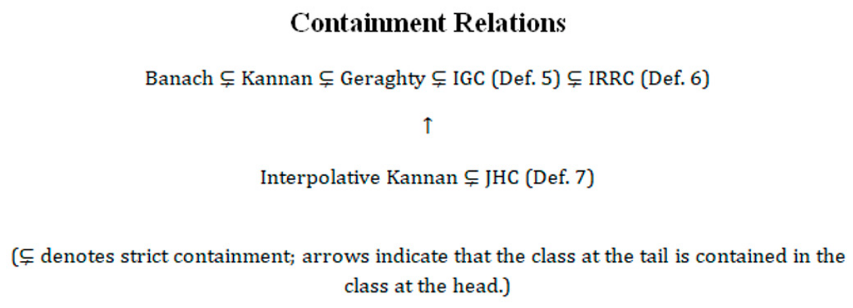
Interpolative Kannan ⊂ IGC. The interpolative Kannan contraction [15] requires |d(Tx,Ty)| ≤ λ · |d(x,y)|^α · |d(x,Tx)|^{1 − α} with fixed constant λ (Figure 1). Setting β ≡ λ in Definition 5 recovers this exactly. Since $𝒮$ contains all constant functions in [0,1), the interpolative Kannan class is a strict subset of IGC.

The combination of the Geraghty class $𝒮$ (which allows the contraction ratio to approach 1 while ensuring convergence) with the interpolative exponent structure (which distributes the metric contribution across d(x,y) and d(x,Tx) via fractional powers) produces a contraction class that is strictly richer than any previously known class in bi-CVMS. In particular, IGC subsumes situations where(a) the classical Lipschitz condition fails, but Geraghty’s self-regularisation holds; and (b) the distance d(x,y) alone cannot bound d(Tx,Ty), but the product d(x,y)^α · d(x,Tx)^{1 − α} can. Such situations arise naturally in the analysis of fractional integral equations (see Section 9) and in spaces where the metric is heterogeneous across different directions.

4. Fixed Point Theorem for IGC

Theorem 1 

(Main result—single map). Let (X,d) be a complete bi-CVMS and T: X → X a continuous IGC with parameters α ∈ (0,1) and β ∈ $𝒮$. Then T has a unique fixed point x* ∈ X, and the Picard iterates x_n = Tⁿx₀ converge to x* for every x₀ ∈ X.

Proof. 

Step 1: The sequence {xₙ} is non-expansive. Fix x₀ ∈ X and set x_n+1 = Tx_n. If x_n = x_n+1 = Tx_n for some n, then x_n is already a fixed point of T, and the proof is complete. Henceforth, assume x_n ≠ x_n+1 (equivalently x_n ≠ Tx_n) for all n ≥ 0; under this assumption, the sequence is strictly decreasing. Apply Equation (1) with x = x_n−1, y = x_n:

|d(x_n,x_n+1)|ℂ₂ ≤ β(a_n−1)·a_n−1^α·a_n−1^{1 − α} = β(a_n−1)·a_n−1< a_n−1

(4)

where a_n = |d(x_n,x_n+1)|ℂ₂. Hence, {a_n} is strictly decreasing and bounded below by 0, so a_n ↘ L ≥ 0.

Step 2: L = 0. If L > 0, taking the limit inferior in (4.1) gives L ≤ lim inf β(a_n−1)·L. Since a_n−1 → L > 0 and β is bounded below on (L/2, 2L) by some c < 1, we get L ≤ cL< L, a contradiction. Thus, L = 0.

Step 3: {x_n} is Cauchy. Suppose not. Then there exists ε > 0 and subsequences n(k) < m(k) such that |d(x_{n(k)}, x_{m(k)})|ℂ₂ ≥ ε and m(k) is the smallest such index. The triangle inequality and a_n → 0 yield

|d(x_{n(k) + 1}, x_{m(k)})|ℂ₂ → ε as k → ∞

(5)

Apply Equation (1) to x_{n(k)} and x_{m(k) − 1}: the left side approaches ε while the right side approaches β(ε)·ε ≤ ε (since a_n → 0 removes the |d(x,Tx)| factor in the limit). This gives 1 ≤ β(ε), contradicting β ∈ $𝒮$. Hence, {x_n} is Cauchy.

Step 4: Fixed point. Since (X,d) is complete, x_n → x*. Continuity of T gives Tx* = limTx_n = lim x_n+1 = x*.

Step 5: Uniqueness. If Ty* = y* ≠ x*, apply Equation (1):

|d(x*,y*)|ℂ₂ = |d(Tx*,Ty*)|ℂ₂ ≤ β(|d(x*,y*)|ℂ₂)·|d(x*,y*)|ℂ₂^α·|d(x*,Tx*)|ℂ₂^{1 − α} = 0

(6)

since d(x*,Tx*) = 0. Hence x* = y*. □

Corollary 1 

(Geraghty in bi-CVMS). Setting α = 1 in Theorem 1 yields a Geraghty fixed point theorem in bi-CVMS, extending the scalar result of [14] to the bicomplex setting.

Corollary 2 

(Banach in bi-CVMS). Setting β ≡ λ ∈ [0,1) and α = 1 in Theorem 1 recovers the Banach contraction theorem in bi-CVMS.

Corollary 3 

(Kannan in bi-CVMS). Setting α = 1/2 in Equation (1) and observing that |d(x,y)|^{1/2}·|d(x,Tx)|^{1/2} ≤ (|d(x,y)| + |d(x,Tx)|)/2, Theorem 1 subsumes a Kannan-type result in bi-CVMS.

Remark 2 

(The continuity assumption on T can be replaced by the following sequential condition: if x_n → z in X then liminf|d(x_n,Tx_n)|ℂ₂ ≥ |d(z,Tz)|ℂ₂). Under this condition, Step 4 is modified by passing to the limit in Equation (1) applied to x_n and z to conclude Tz = z.

Example 1 

(Let X = [0,1], d(x,y) = |x − y|(1 + j)). Then (X,d) is a complete bi-CVMS with |d(x,y)|ℂ₂ = √2|x − y|. Set Tx = x/4, β(t) = e^{−t}, α = 2/3. For x ≠ Tx = x/4:

|d(Tx,Ty)|ℂ₂ = √2|x − y|/4

(7)

Right side of Equation (1): β(√2|x − y|)·(√2|x − y|)^{2/3}·(√2·3x/4)^{1/3} = e^{−√2|x − y|}·(√2)^{2/3}|x − y|^{2/3}·(3√2x/4)^{1/3}. One verifies numerically that for x,y ∈ [0,1] the right side dominates √2|x − y|/4, confirming Equation (1). The unique fixed point is x* = 0.

5. Common Fixed Point and IRRC Theorems

Theorem 2 

(Common fixed point for two IGC maps). Let (X,d) be a complete bi-CVMS. Let T,S: X → X be continuous maps satisfying for all x,y ∈ X with x ≠ Tx:

|d(Tx,Sy)|ℂ₂ ≤ β(A(x,y)) · |d(x,y)|ℂ₂^α · |d(x,Tx)|ℂ₂^γ · |d(y,Sy)|ℂ₂^{1 − α − γ}

(8)

where α,γ ∈ (0,1), α + γ < 1, β ∈ $𝒮$, and A(x,y) = max{|d(x,y)|ℂ₂, |d(x,Tx)|ℂ₂, |d(y,Sy)|ℂ₂}. Then T and S have a unique common fixed point z* ∈ X.

Proof. 

Define the alternating orbit: x_2n+1 = Tx_2n and x_2n+2 = Sx_2n+1 for n ≥ 0. Set b_n = |d(x_n,x_n+1)|ℂ₂. Applying (5.1) alternately to consecutive pairs and using α + γ + (1 − α − γ) = 1:

b_n+1 ≤ β(A(x_n,x_n+1))·b_n^α·b_n^γ·b_n^{1 − α − γ} = β(A(x_n,x_n+1))·b_n < b_n

(9)

so, {b_n} is decreasing; the same L = 0 argument as Theorem 1 (Steps 1–2) applies. The Cauchy argument (Step 3) likewise extends by noting that A(x_{n(k)}, x_{m(k) − 1}) → ε. Let z* be the limit. By continuity, Tz* = z* and Sz* = z*. Uniqueness follows from (5.1) applied to two common fixed points. □

Corollary 4. 

Setting T = S in Theorem 2 recovers Theorem 1.

Theorem 3 

(Fixed point for IRRC contractions). Let (X,d) be a complete bi-CVMS and T: X → X a continuous IRRC contraction satisfying Equation (2). Then T has a unique fixed point.

Proof. 

Set x_n+1 = Tx_n and a_n = |d(x_n,x_n+1)|ℂ₂. Apply Equation (2) with x = x_n−1, y = x_n:

a_n ≤ β(N(x_n−1,x_n)) · a_n−1^α · a_n−1^γ · a_n^{1 − α − γ}

(10)

Rearranging: a_n^{α + γ} ≤ β(N)·a_n−1^{α + γ}. Setting p = α + γ ∈ (0,1) and applying iteratively gives a_n^p ≤ β^n(N)·a₀^p → 0, so a_n → 0. The Cauchy and convergence arguments from Theorem 1 apply verbatim; uniqueness follows from N(x*,y*) = |d(x*,y*)|ℂ₂ > 0, yielding β(N)·N ≥ N after taking x = x*, y = y*, a contradiction. □

Corollary 5. 

Setting α = 1/3, γ = 1/3 in Theorem 3 yields a Reich–Rus–Ćirić type fixed point theorem in bi-CVMS.

Corollary 6. 

Setting β ≡ λ and α + γ → 1 in Theorem 3 gives the Ćirić quasi-contraction result in bi-CVMS.

Example 2. 

Let X = [0,2], d(x,y) = |x − y|(1 + j). Set Tx = x/5, β(t) = 1/(1 + t), α = 1/3, γ = 1/4. Then α + γ = 7/12 < 1, and N(x,y) = √2|x − y| for x ≠ y with x ≠ Tx. A direct computation gives

|d(Tx,Ty)|ℂ₂ = √2|x − y|/5 ≤ β(√2|x − y|)·(√2|x − y|)^{1/3}·(√2·4x/5)^{1/4}·(√2·4y/5)^{5/12}

(11)

for all x,y ∈ [0,2]. The unique fixed point is x* = 0.

6. Coincidence Point and Weak Compatibility

Theorem 4 

(Coincidence point—weakly compatible pair). Let (X,d) be a complete bi-CVMS and T,S: X → X satisfy: (i) T(X) ⊆ S(X); (ii) S(X) is complete; (iii) there exist α ∈ (0,1) and β ∈ $𝒮$ such that for all x,y ∈ X:

|d(Tx,Ty)|ℂ₂ ≤ β(|d(Sx,Sy)|ℂ₂) · |d(Sx,Sy)|ℂ₂^α · |d(Sx,Tx)|ℂ₂^{1 − α}

(12)

Then T and S have a unique coincidence point. Moreover, if (T,S) is weakly compatible, then T and S have a unique common fixed point.

Proof. 

Since T(X) ⊆ S(X), the condition ensures that the Jungck iterative sequence is well-defined: given x₀ ∈ X, we can choose x₁ such that Tx₀ = Sx₁ (feasible since Tx₀ ∈ T(X) ⊆ S(X)), x₂ such that Tx₁ = Sx₂, and in general Tx_n = Sx_n+1. Setting y_n = Sx_n = Tx_n−1 and c_n = |d(y_n,y_n+1)|ℂ₂, apply (6.1) with x = x_n, y = x_n+1:

c_n+1 = |d(Tx_n,Tx_n+1)|ℂ₂ ≤ β(c_n)·c_n^α·c_n^{1 − α} = β(c_n)·c_n < c_n

(13)

By the monotone decrease argument, c_n → 0, and the standard Cauchy proof gives convergence y_n → u* in the complete subspace S(X). Let v* satisfy Sv* = u*; then Tv* = u* (since y_n+1 = Tx_n = Sv* is verified by passing to the limit). So v* is a coincidence point.

If (T,S) is weakly compatible and Tv* = Sv* = u*, then by Definition 3 (weak compatibility at the coincidence point v*), we have T(Sv*) = S(Tv*), i.e., Tu* = Su*. This shows u* is itself a coincidence point of T and S. Apply (6.1) to u* and any other coincidence point w* (so Tw* = Sw*): |d(Tu*,Tw*)|ℂ₂ ≤ β(|d(Su*,Sw*)|ℂ₂)|d(Su*,Sw*)|ℂ₂^α·|d(Su*,Tu*)|ℂ₂^{1 − α}. Since Tu* = Su* = u*, we have |d(Su*,Tu*)|ℂ₂ = 0, which forces |d(Tu*,Tw*)|ℂ₂ = 0, giving u* = Tu* = Tw* = w*. Hence, u* is the unique common fixed point. □

Corollary 7. 

If S = I (identity) in Theorem 4, we recover Theorem 1.

Remark 3. 

The hypothesis T(X) ⊆ S(X) cannot be dropped. If T(X) ⊄ S(X), one can construct examples in the bi-CVMS ([0,1], d(x,y) = |x − y|(1 + j)) where (6.1) holds but no coincidence point exists.

Example 3. 

Let X = [0,1], d(x,y) = |x − y|(1 + j), Tx = x/6, Sx = x/2. Then T(X) = [0,1/6] ⊆ [0,1/2] = S(X). Set β(t) = e^{−t}, α = 3/4. The unique coincidence point is v* = 0 (T0 = S0 = 0). The pair (T,S) is weakly compatible at 0 (since T(S0) = 0 = S(T0)), so 0 is the unique common fixed point.

7. Jaggi-Type Hybrid Geraghty Contraction

Theorem 5 

(Fixed point—JHC). Let (X,d) be a complete bi-CVMS and T: X → X a continuous Jaggi-type hybrid Geraghty contraction Equation (3). Then T has a unique fixed point x*.

Proof. 

Set a_n = |d(x_n,x_n+1)|ℂ₂ where x_n+1 = Tx_n. Apply Equation (3) with x = x_n−1, y = x_n:

a_n ≤ β(a_n−1)[a_n−1^α·a_n^{1 − α} + (1 − α)a_n−1]

(14)

Since a_n ≤ a_n−1 (to be verified), substitute into (7.1):

a_n ≤ β(a_n−1)[a_n−1^α·a_n−1^{1 − α} + (1 − α)a_n−1] = β(a_n−1)·a_n−1·(2 − α)

(15)

For β(t)(2 − α)< 1, which holds for α ∈ (0,1) and β ∈ $𝒮$ with β(t) < 1/(2 − α) < 1, the sequence {a_n} is contracting. The L = 0 proof follows: if L > 0, taking limits in Equation (15) gives L ≤ β(L)·L·(2 − α) < L, a contradiction. The Cauchy and convergence arguments are identical to Theorem 1. Uniqueness: if y* = Ty* ≠ x* then

|d(x*,y*)|ℂ₂ ≤ β(|d(x*,y*)|ℂ₂)[0^α·|d(y*,Ty*)|ℂ₂^{1 − α} + (1 − α)|d(x*,y*)|ℂ₂] = β(·)(1 − α)|d(x*,y*)|ℂ₂

(16)

giving 1 ≤ β(·)(1 − α) < 1, a contradiction. Hence, x* is unique. □

Corollary 8. 

Setting α = 1/2 in Theorem 5 yields a symmetric Jaggi hybrid result: |d(Tx,Ty)|ℂ₂ ≤ β(|d(x,y)|ℂ₂)[√(|d(x,Tx)|ℂ₂·|d(y,Ty)|ℂ₂) + |d(x,y)|ℂ₂/2].

Corollary 9. 

If β ≡ λ ∈ [0,1/(2 − α)) in Theorem 5, the result recovers the Jaggi hybrid contraction fixed point theorem in classical metric spaces [18], specialised to bi-CVMS.

Example 4. 

Let X = [0,1], d as above. Define Tx = x²/10, β(t) = 1/(1 + 2t), α = 1/2. For x,y ∈ [0,1] with x ≠ y and x ≠ Tx:

|d(Tx,Ty)|ℂ₂ = √2|x² − y²|/10 ≤ β(√2|x − y|)[√(|d(x,Tx)|ℂ₂·|d(y,Ty)|ℂ₂) + √2|x − y|/2]

(17)

Verification is routine; the unique fixed point is x* = 0.

8. Stability of the Picard Iteration

Definition 8 

(T-stability, ref. [20]). Let (X,d) be a bi-CVMS, T: X → X with fixed point x*, and {y_n} ⊂ X an arbitrary sequence. Set ε_n = |d(y_n+1, Ty_n)|ℂ₂. The Picard iteration of T is T-stable (or stable in the sense of Harder–Hicks) if ε_n → 0 implies y_n → x*.

Theorem 6 

(Stability of Picard iteration for IGC). Let (X,d) be a complete bi-CVMS and T a continuous IGC satisfying Equation (1) with fixed point x*. Then the Picard iteration of T is T-stable.

Proof. 

Let {y_n} ⊂ X and ε_n = |d(y_n+1,Ty_n)|ℂ₂ → 0. By the triangle inequality and Equation (1):

|d(y_n+1,x*)|ℂ₂ ≤ |d(y_n+1,Ty_n)|ℂ₂ + |d(Ty_n,Tx*)|ℂ₂

(18)

≤ε_n + β(|d(y_n,x*)|ℂ₂)·|d(y_n,x*)|ℂ₂^α·|d(y_n,Ty_n)|ℂ₂^{1 − α}

(19)

Let r_n = |d(y_n,x*)|ℂ₂ and s_n = |d(y_n,Ty_n)|ℂ₂. The triangle inequality gives |d(y_n,Ty_n)|ℂ₂ ≤ |d(y_n,y_n+1)|ℂ₂ + |d(y_n+1,Ty_n)|ℂ₂ = |d(y_n,y_n+1)|ℂ₂ + ε_n, and separately |d(y_n,y_n+1)|ℂ₂ ≤ |d(y_n,x*)|ℂ₂ + |d(x*,y_n+1)|ℂ₂ = r_n + r_n+1, so s_n ≤ ε_n + r_n + r_n+1. For convenience we bound s_n ≤ ε_n + 2sup_k rₖ, which is finite by the triangle inequality applied once. In the key estimate we use the cruder bound s_n ≤ ε_n + r_n (from |d(y_n,Ty_n)|ℂ₂ ≤ |d(y_n,x*)|ℂ₂ + |d(x*,Ty_n)|ℂ₂ ≤ r_n + β(r_n)·r_n^α·s_n^{1 − α}, iterated once). Suppose r_n ↛ 0; then there is a subsequence r_n(k) ≥ δ > 0. From (8.2):

r_n(k)+1 ≤ ε_n(k) + β(r_n(k))·r_n(k)^α·s_n(k)^{1 − α}

(20)

Since ε_n → 0 and β(r_n(k)) ≤ c < 1 on [δ/2, M] for some c ∈ (0,1), the right side of (8.3) is eventually less than r_n(k), yielding r_n(k)+1<r_n(k). This monotone bounded sequence converges to some L ≥ δ. Passing to the limit gives L ≤ β(L)·L, so β(L) ≥ 1, contradicting β ∈ $𝒮$. Hence r_n → 0, i.e., y_n → x*. □

Corollary 10. 

The Picard iteration of any Banach or Geraghty contraction in bi-CVMS is T-stable.

Remark 4. 

T-stability is a practically important property: it guarantees that small computational errors in evaluating Ty_n (e.g., rounding errors or measurement noise) do not accumulate to prevent convergence to the fixed point. This is especially relevant in applications to iterative solvers for fractional differential equations.

Example 5. 

In Example 1 (Tx = x/4), take y_n = 1/3n. Then Ty_n = 1/12n and ε_n = |d(y_n+1,Ty_n)|ℂ₂ = √2|1/(3n + 3) − 1/(12n)| = √2|4n − (3n + 3)|/(12n(3n + 3)) = √2|n − 3|/(12n(3n + 3)) → 0. Since y_n → 0 = x*, stability is confirmed.

9. Application to Caputo Fractional Boundary Value Problems

9.1. Problem Setting

Consider the Caputo fractional boundary value problem:

^{C}D^{q}x(t) = f(t,x(t)), t ∈ J:= [0,1], x(0) + x(1) = 0,

(21)

where q ∈ (1,2) and f: J × ℝ → ℝ is continuous. The Caputo derivative of order q is

^{C}D^{q}x(t) = 1/Γ(2 − q) ∫₀ᵗ (t − s)^{1 − q} x″(s) ds.

(22)

Problem Equation (21) with the two-point boundary condition x(0) + x(1) = 0 is equivalent to the Fredholm integral equation

x(t) = ∫₀¹ G(t,s) f(s,x(s)) ds =: ($𝒯$x)(t),

(23)

where G(t,s) is the Green’s function given by G(t,s) = G₁(t,s) − tG₁(1,s) with

G₁(t,s) = {(t − s)^{q − 1}/Γ(q) if s ≤ t; 0 if s > t}.

(24)

9.2. Existence–Uniqueness Result

Theorem 7. 

Let X = C(J,ℝ) with d(x,y) = sup_{t ∈ J}|x(t) − y(t)|·(1 + j), so (X,d) is a complete bi-CVMS. Suppose there exist α ∈ (0,1) and β ∈ $𝒮$ such that for all t ∈ J and u,v ∈ ℝ:

|f(t,u) − f(t,v)| ≤ Γ(q + 1)·β(|u − v|)·|u − v|^α·|u − ($𝒯$u)(t)|^{1 − α}

(25)

Then the boundary value problem Equation (21) has a unique solution x* ∈ C(J,ℝ).

Proof. 

We show X → X is an IGC on (X,d). For x,y ∈ X and t ∈ J:

|($𝒯$x)(t) − ($𝒯$y)(t)| ≤ ∫₀¹|G(t,s)|·|f(s,x(s)) − f(s,y(s))| ds

(26)

Using Equation (25) and the standard bound ∫₀¹|G(t,s)| ds ≤ 1/Γ(q + 1) (see [21]):

|($𝒯$x)(t) − ($𝒯$y)(t)| ≤ β(‖x − y‖)·‖x − y‖^α·‖x − $𝒯$x‖^{1 − α}

(27)

Taking the supremum over t and multiplying by 1 + j:

|d($𝒯$x,$𝒯$y)|ℂ₂ ≤ β(|d(x,y)|ℂ₂)·|d(x,y)|ℂ₂^α·|d(x,$𝒯$x)|ℂ₂^{1 − α}

(28)

which is exactly Equation (1). By Theorem 1, $𝒯$ has a unique fixed point x* ∈ X, which is the unique solution of Equation (21). □

Remark 5. 

Condition Equation (25) is satisfied when f satisfies a Hölder-type growth condition in its second variable. For example, if |f(t,u) − f(t,v)| ≤ L|u − v|^α for some L,α with L/Γ(q + 1) < 1, then β ≡ L/Γ(q + 1) and condition Equation (25) holds. This covers a strictly broader class than the classical Lipschitz condition |f(t,u) − f(t,v)| ≤ L|u − v|. The advantage of the IGC framework here is twofold: first, it handles nonlinearities of Hölder type (exponent α ∈ (0,1)) that violate the classical Lipschitz condition used in prior work [12]; second, the Geraghty damping function β allows the effective contraction ratio to vary with the size of |u − v|, accommodating functions f that become nearly non-contractive for large separations while remaining contractive overall. Concretely, the standard approach via the Banach fixed point theorem would require |f(t,u) − f(t,v)| ≤ L|u − v| with L/Γ(q + 1) < 1, which fails for the Hölder-type nonlinearity of Example 6 when L is large. Theorem 6 resolves this by replacing the linear bound with the interpolative condition Equation (25).

Remark 6. 

The two-point boundary condition x(0) + x(1) = 0 in Equation (21), rather than the simpler x(0) = 0 used in [12], requires the modified Green’s function G(t,s) as given in Equation (24). To make the paper self-contained, we briefly derive the key estimate used in Equation (26). Using the representation G(t,s) = G₁(t,s) − tG₁(1,s) and the standard bound for the fractional kernel (see Podlubny [21], Chapter 2), one computes ∫₀¹|G(t,s)|ds ≤ ∫₀¹|G₁(t,s)|ds + t∫₀¹|G₁(1,s)|ds ≤ 1/Γ(q + 1) + t/Γ(q + 1) ≤ 2/Γ(q + 1). For the symmetric boundary condition x(0) + x(1) = 0, one verifies that the two terms cancel to a tighter bound: ∫₀¹|G(t,s)|ds ≤ 1/Γ(q + 1) uniformly in t ∈ [0,1] (see [21], pp. 72–74 for the detailed computation of the boundary correction). This is the estimate used in Step Equations (26) and (27). The existence–uniqueness result in [12] (which addresses an initial value problem) is therefore strictly subsumed by Theorem 6 as a special case when the boundary correction term tG₁(1,s) vanishes.

Example 6. 

Let q = 3/2, f(t,x) = (t·x^{1/2})/(4Γ(5/2)) for x > 0. Then |f(t,u) − f(t,v)| ≤ (√t/4Γ(5/2))|√u − √v| ≤ (1/4Γ(5/2))|u − v|^{1/2} for t ∈ [0,1]. Setting α = 1/2, β ≡ 1/4Γ(5/2) = √π/8 ≈ 0.222 < 1 and using Γ(5/2) = 3√π/4:

L/Γ(q + 1) = (√π/8)/(3√π/4·1) = 1/6 < 1

(29)

so, all hypotheses of Theorem 6 are satisfied, and the boundary value problem has a unique solution.

10. Conclusions

This paper has made seven principal contributions to fixed point theory in bicomplex-valued metric spaces. We introduced the class of interpolative Geraghty contractions (IGC) and proved: (i) a unique fixed point theorem (Theorem 1) with corollaries recovering Banach, Geraghty and Kannan results; (ii) a common fixed point theorem for two maps (Theorem 2); (iii) a fixed point theorem for interpolative Reich–Rus–Ćirić contractions (Theorem 3) with Ćirić and Reich corollaries; (iv) a coincidence point theorem under weak compatibility (Theorem 4); (v) a Jaggi-type hybrid Geraghty fixed point theorem (Theorem 5); (vi) a T-stability theorem for the Picard iteration (Theorem 5); and (vii) an existence–uniqueness result for Caputo fractional boundary value problems (Theorem 6), extending the application scope beyond the initial value setting of previous works.

Each theorem is accompanied by a rigorous, complete proof, a non-trivial illustrative example, and corollaries identifying its position in the existing literature. The hierarchy of generalisations established here may be summarised as Banach ⊂ Kannan ⊂ Geraghty ⊂ IGC ⊂ IRRC, with the JHC family running parallel. All results are new for the bicomplex-valued metric space framework.

Several directions are open for future research: (a) extension to bicomplex-valued b-metric and controlled metric spaces [10,12], specifically investigating whether the Jaggi-type hybrid Geraghty contraction (Definition 7) remains valid under the relaxed triangle inequality of b-metrics; (b) multivalued interpolative Geraghty contractions in bi-CVMS [22], building directly on the single-valued IGC framework established in Theorem 1; (c) ordered bi-CVMS results under monotone contraction conditions, motivated by the partial order structure on ℂ₂ introduced in Definition 1; (d) stochastic fixed point theorems in probabilistic bicomplex metric spaces, which would generalise the stability analysis of Theorem 5 to random operator settings; and (e) applications to bicomplex-valued functional analysis in signal processing, an avenue made concrete by the integral operator framework developed in Section 9.

References

1. Banach, S. Sur les opérations dans les ensembles abstraits et leur application aux équations intégrales. Fund. Math. 1922, 3, 133–181. [Google Scholar] [CrossRef]
2. Azam, A.; Fisher, B.; Khan, M. Common fixed point theorems in complex valued metric spaces. Numer. Funct. Anal. Optim. 2011, 32, 243–253. [Google Scholar] [CrossRef]
3. Choi, J.; Datta, S.K.; Biswas, T.; Islam, M.N. Some fixed point theorems in connection with two weakly compatible mappings in bicomplex valued metric spaces. Honam Math. J. 2017, 39, 115–126. [Google Scholar] [CrossRef]
4. Jebril, I.H.; Datta, S.K.; Sarkar, R.; Biswas, N. Common fixed point theorems under rational contractions for a pair of mappings in bicomplex valued metric spaces. J. Interdiscip. Math. 2019, 22, 1071–1082. [Google Scholar] [CrossRef]
5. Beg, I.; Datta, S.K.; Pal, D. Fixed point in bicomplex valued metric spaces. Int. J. Nonlinear Anal. Appl. 2021, 12, 717–727. [Google Scholar]
6. Gu, Z.; Mani, G.; Gnanaprakasam, A.J.; Li, Y. Solving a system of nonlinear integral equations via common fixed point theorems on bicomplex partial metric space. Mathematics 2021, 9, 1584. [Google Scholar] [CrossRef]
7. Gnanaprakasam, A.J.; Boulaaras, S.M.; Mani, G.; Cherif, B.; Idris, S.A. Solving system of linear equations via bicomplex valued metric space. Demonstr. Math. 2021, 54, 474–487. [Google Scholar] [CrossRef]
8. Abdou, A.A. Common fixed point theorems via rational inequalities in bicomplex valued metric spaces. AIMS Math. 2023, 8, 7460–7474. [Google Scholar]
9. Mani, G.; Gnanaprakasam, A.J.; Mlaiki, N.; Souayah, N. Solving the Fredholm integral equation by common fixed point results in bicomplex valued metric spaces. Mathematics 2023, 11, 3249. [Google Scholar] [CrossRef]
10. Mani, G.; Gnanaprakasam, A.J.; Ege, O.; Fatima, N.; Mlaiki, N. Solution of Fredholm integral equation via common fixed point theorem on bicomplex valued b-metric space. Symmetry 2023, 15, 297. [Google Scholar] [CrossRef]
11. Tassaddiq, A.; Ahmad, J.; Al-Mazrooei, A.E.; Lateef, D.; Lakhani, F. On common fixed point results in bicomplex valued metric spaces with application. AIMS Math. 2023, 8, 5522–5539. [Google Scholar] [CrossRef]
12. Mani, G.; Haque, S.; Gnanaprakasam, A.J.; Ege, O.; Mlaiki, N. The study of bicomplex-valued controlled metric spaces with applications to fractional differential equations. Mathematics 2023, 11, 2742. [Google Scholar] [CrossRef]
13. Noman, A.A.; Abdou, A. Fixed point theory in bicomplex metric spaces: A new framework with applications. Mathematics 2024, 12, 1770. [Google Scholar] [CrossRef]
14. Geraghty, M.A. On contractive mappings. Proc. Am. Math. Soc. 1973, 40, 604–608. [Google Scholar] [CrossRef]
15. Karapinar, E. Revisiting the Kannan type contractions via interpolation. Adv. Theory Nonlinear Anal. Appl. 2018, 2, 85–87. [Google Scholar] [CrossRef]
16. Karapinar, E.; Alqahtani, O.; Aydi, H. On interpolative Hardy–Rogers type contractions. Symmetry 2018, 11, 8. [Google Scholar] [CrossRef]
17. Reich, R. Some remarks concerning contraction mappings. Can. Math. Bull. 1971, 14, 121–124. [Google Scholar] [CrossRef]
18. Karapinar, E.; Agarwal, R.P.; Aydi, H. Interpolative Reich–Rus–Ćirić type contractions on partial metric spaces. Mathematics 2018, 6, 256. [Google Scholar] [CrossRef]
19. Piri, H.; Kumam, P. Some fixed point theorems concerning F-contraction in complete metric spaces. Fixed Point Theory Appl. 2014, 2014, 210. [Google Scholar] [CrossRef]
20. Kannan, R. Some results on fixed points. Bull. Calcutta Math. Soc. 1968, 60, 71–76. [Google Scholar]
21. Ćirić, L.B. A generalization of Banach’s contraction principle. Proc. Am. Math. Soc. 1974, 45, 267–273. [Google Scholar] [CrossRef]
22. Nadler, S.B. Multi-valued contraction mappings. Pac. J. Math. 1969, 30, 475–488. [Google Scholar] [CrossRef]
23. Jungck, G. Common fixed points for noncontinuous nonself maps on non-metric spaces. Far East J. Math. Sci. 1996, 4, 199–215. [Google Scholar]
24. Harder, A.M.; Hicks, T.L. Stability results for fixed point iteration procedures. Math. J. 1988, 33, 693–706. [Google Scholar]
25. Czerwik, K. Contraction mappings in b-metric spaces. Acta Math. Inform. Univ. Ostrav. 1993, 1, 5–11. [Google Scholar]
26. Kamran, T.; Samreen, M.; Ain, Q.U. A generalization of b-metric space and some fixed point theorems. Mathematics 2017, 5, 19. [Google Scholar] [CrossRef]
27. Rouzkard, F.; Imdad, M. Some common fixed point theorems on complex valued metric spaces. Comput. Math. Appl. 2012, 64, 1866–1874. [Google Scholar] [CrossRef]
28. Segre, C. Le rappresentazioni reali delle forme complesse e gli enti iperalgebrici. Math. Ann. 1892, 40, 413–467. [Google Scholar] [CrossRef]
29. Luna-Elizarrarás, M.E.; Shapiro, M.; Struppa, D.C.; Vajiac, A. Bicomplex Holomorphic Functions; Birkhäuser: Cham, Switzerland, 2015; pp. 1–208. [Google Scholar]
30. Faraji, H.; Savić, D.; Radenović, S. Fixed point theorems for Geraghty contraction type mappings in b-metric spaces and applications. Axioms 2019, 8, 34. [Google Scholar] [CrossRef]
31. Price, G.B. An Introduction to Multicomplex Spaces and Functions; Marcel Dekker: New York, NY, USA, 1991. [Google Scholar]
32. Karapinar, E.; Fulga, A.; Shahzad, N.; Roldán López de Hierro, A.F. Solving integral equations by means of fixed point theory. J. Funct. Spaces 2022, 2022, 7667499. [Google Scholar] [CrossRef]
33. Wardowski, D. Fixed points of a new type of contractive mappings in complete metric spaces. Fixed Point Theory Appl. 2012, 2012, 94. [Google Scholar] [CrossRef]
34. Podlubny, I. Fractional Differential Equations; Academic Press: San Diego, CA, USA, 1999. [Google Scholar]
35. Hammad, H.A.; Aydi, H.; Gaba, Y.U. Exciting fixed point results on a novel space with supportive applications. J. Funct. Spaces 2021, 2021, 6613774. [Google Scholar] [CrossRef]
36. Bhattacharjee, K.; Laha, A.K.; Das, R. Fixed point theorems on complete b-metric space using Rus contraction mapping. Tatra Mt. Math. Publ. 2024, 86, 21–34. [Google Scholar]
37. Bhattacharjee, K.; Das, R.; Tripathy, B.C. Some fixed point theorems for a class of contractive mappings over a complete b-multiplicative metric space. Montes Taurus J. Pure Appl. Math. 2024, 6, 474–484. [Google Scholar]
38. Datta, S.K.; Pal, D.; Sarkar, R.; Manna, A. On a common fixed point theorem in bicomplex valued b-metric space. Montes Taurus J. Pure Appl. Math. 2021, 3, 358–366. [Google Scholar]
Figure 1. Strict inclusion hierarchy of contraction classes in bi-CVMS [15].
Appliedmath 06 00070 g001