On Efficient Two-Stage Implicit Schemes for Fractional Differential Equations: Parallel OpenMP-Type Execution and Learning-Guided Initializations

Abstract

This paper presents a hybrid two-stage implicit scheme for the numerical solution of fractional initial value problems involving Caputo derivatives. The proposed formulation incorporates the nonlinear source term directly into the time-stepping procedure, leading to improved stability and accuracy compared with classical fractional implicit schemes. The resulting nonlinear systems are solved using a parallel iterative strategy based on the Weierstrass-type method, combined with OpenMP-style parallelization to ensure efficient workload distribution and accelerated convergence. In addition, a data-driven module is introduced to generate high-quality initial guesses, thereby enhancing the robustness and efficiency of the nonlinear solver. The main contributions include the development of a unified fractional-parallel-data-driven framework, improved stability properties with enlarged real-axis stability regions, and reduced computational cost through parallel implementation and informed initialization. A theoretical analysis establishes consistency, boundedness, and convergence under standard Lipschitz assumptions. Numerical experiments on representative fractional models demonstrate that the proposed schemes achieve higher accuracy and improved efficiency compared with classical implicit methods, with significant reductions in error and iteration counts. The ANN-enhanced variant further attains near machine-precision accuracy for a range of fractional orders. Overall, the proposed approach provides a robust and scalable computational framework for the efficient solution of nonlinear fractional dynamical systems.

1. Introduction

Fractional differential equations (FDEs) provide a powerful mathematical framework for modeling memory and hereditary effects in complex dynamical systems. In contrast to classical integer-order models, fractional operators incorporate nonlocal temporal behavior, making them particularly suitable for describing anomalous diffusion, viscoelasticity, bioengineering processes, and nonlinear transport phenomena [1,2,3,4]. From a numerical perspective, effectively capturing these nonlocal features remains a key challenge. In this work, we develop a discretization and solution strategy that explicitly accounts for the memory-dependent structure of fractional models at the discrete level. The proposed approach aims to improve the stability and accuracy of numerical solutions, particularly in the presence of nonlinear dynamics. In particular, the proposed approach differs from standard fractional schemes by embedding nonlinear effects directly into the time-stepping formulation.

Among the various definitions of fractional derivatives, the Caputo derivative is widely adopted due to its compatibility with classical initial conditions. Consider the following fractional initial value problem (FIVP):

$$\left\{\begin{array}{cc}{}^c\wp _{x_0}^{\varphi }g\left(x\right)=f(x,g\left(x\right)), \hfill & x\in (x_0,T],\hfill \\ g^{\left(k\right)}\left(x_0\right)=g_0^{\left(k\right)}, \hfill & k=0,1,\dots ,m-1,\hfill \end{array}\right.$$

(1)

where $m-1<\varphi <m$, $m\in \mathbb{N}$, $g:[x_0,T]\to {\mathbb{R}}^d$, and  $f:[x_0,T]\times {\mathbb{R}}^d\to {\mathbb{R}}^d$ is a nonlinear mapping. Here, ${}^c\wp _{x_0}^{\varphi }$ denotes the Caputo fractional differential operator of order $\varphi \in (m-1,m)$.

For $g\in C^m[x_0,T]$, the Caputo fractional derivative ${}^c\wp _{x_0}^{\varphi }:C^m[x_0,T]\to C[x_0,T]$ is defined by [5]:

$${}^c\wp _{x_0}^{\varphi }g\left(x\right)={\displaystyle \frac{1}{\mathrm{\Gamma }(m-\varphi )}}{\int }_{x_0}^x{(x-s)}^{m-\varphi -1}{g}^{\left(m\right)}\left(s\right) ds,\hspace{1em}x>x_0.$$

(2)

For $\varphi \in (0,1)$, this expression reduces to:

$${}^c\wp _{x_0}^{\varphi }g\left(x\right)={\displaystyle \frac{1}{\mathrm{\Gamma }(1-\varphi )}}{\int }_{x_0}^x{(x-s)}^{-\varphi } g^{\prime }\left(s\right) ds.$$

(3)

Here, $\mathrm{\Gamma }(·)$ denotes the Gamma function:

$$\mathrm{\Gamma }\left(\gamma \right)={\int }_0^{\infty }{e}^{-u}{u}^{\gamma -1} du,\hspace{1em}\gamma >0.$$

The Caputo derivative is adopted due to its compatibility with classical initial conditions. In particular, it preserves the property that the derivative of a constant is zero, ensuring consistency with classical differential calculus and facilitating the formulation of physically meaningful initial value problems.

In contrast, alternative fractional operators such as the Caputo–Fabrizio and Atangana–Baleanu derivatives do not preserve this classical property in the same form, which may complicate the formulation of standard initial value problems. The Caputo operator, by comparison, retains compatibility with classical initial conditions and features a weakly singular kernel, providing a consistent framework for modeling hereditary dynamical systems.

The operator ${}^c\wp _{x_0}^{\varphi }$ is linear and satisfies:

• Linearity:

  $${}^c\wp _{x_0}^{\varphi } \left(m_1{g}_1+m_2{g}_2\right)=m_1{}^c\wp _{x_0}^{\varphi }{g}_1+m_2{}^c\wp _{x_0}^{\varphi }{g}_2.$$
• Power function: for $\beta >\varphi -1$:

  $${}^c\wp _{x_0}^{\varphi }{(x-x_0)}^{\beta }={\displaystyle \frac{\mathrm{\Gamma }(\beta +1)}{\mathrm{\Gamma }(\beta +1-\varphi )}}{(x-x_0)}^{\beta -\varphi }.$$
• Constant function:

  $${}^c\wp _{x_0}^{\varphi }C=0.$$

Moreover, if $\varphi =m\in \mathbb{N}$, then ${}^c\wp _{x_0}^{m}g\left(x\right)=g^{\left(m\right)}\left(x\right)$; so, the operator coincides with the classical derivative. These properties make the Caputo derivative a natural choice for the formulation and numerical treatment of fractional initial value problems considered in this work.

1.1. Literature Review and Motivation

Classical numerical approaches for fractional initial value problems include the L1 scheme [6], fractional Adams–Bashforth–Moulton methods [7], Grünwald–Letnikov discretizations [8], and various implicit predictor–corrector strategies [9,10,11,12]. More recent developments have focused on improved discretization techniques for Caputo-type models, including fast convolution methods, spectral approaches, and higher-order fractional schemes [13,14,15,16].

In parallel, significant effort has been devoted to the development of efficient nonlinear solvers for fractional systems, particularly Newton-type and modified Newton iterations, as well as parallel implementations aimed at reducing computational cost [17,18,19,20]. Despite these advances, achieving a balance between accuracy, stability, and computational efficiency remains challenging, especially for strongly nonlinear problems.

While these methods are consistent and convergent under suitable regularity assumptions, they often exhibit several limitations:

−

Restrictive stability regions for stiff nonlinear systems;

−

Reduced convergence rates in the presence of strong nonlinearities;

−

$\mathrm{𝒪}\left(N^2\right)$ memory and computational cost due to the history term;

−

Limited scalability for large-scale or parallel simulations.

Implicit fractional schemes [21] can improve stability, but require the solution of nonlinear algebraic systems at each time step. In practice, these systems are typically solved using classical Newton-type iterations [22], often without optimized initialization or explicit workload balancing [23,24], which may lead to slow convergence or increased computational cost [25].

Although substantial progress has been made, a unified framework that simultaneously integrates (i) enhanced nonlinear discretization, (ii) efficient parallel solution strategies, and (iii) data-driven initialization mechanisms remains largely unexplored in the context of fractional problems.

1.2. Research Gap

Despite the progress outlined above, several specific limitations remain in the current literature:

• In many fractional implicit schemes, the nonlinear source term is treated explicitly or semi-implicitly, which may degrade stability and accuracy in strongly nonlinear regimes.
• The nonlinear algebraic systems arising at each time step are typically solved using standard iterative methods, often without informed initialization or explicit convergence control, leading to unnecessary computational overhead.
• Although parallel implementations have been explored, the combined effects of workload distribution, solver parameter tuning, and nonlinear stage efficiency have not been systematically integrated within a unified framework for fractional problems.

These observations motivate the development of a mathematically grounded and computationally efficient hybrid framework that integrates nonlinear discretization, parallel solution strategies, and informed initialization within a unified formulation.

1.3. Main Contributions

To address the challenges outlined above, this work introduces a hybrid two-stage implicit framework for fractional initial value problems with the following main contributions:

−

A two-stage implicit fractional discretization that embeds nonlinear source effects directly within the time-stepping formulation, enhancing robustness in nonlinear regimes.

−

A theoretical analysis establishing consistency, boundedness, and convergence of the proposed scheme under standard smoothness and Lipschitz assumptions.

−

A parallel iterative solution strategy implemented in OpenMP, designed to improve workload distribution and convergence efficiency in the nonlinear stage.

−

The incorporation of a data-informed initialization mechanism to provide improved starting guesses and support solver parameter tuning.

−

A comprehensive numerical assessment, including error metrics and real-axis stability analysis, demonstrating the performance of the proposed method relative to classical fractional implicit schemes.

Overall, the proposed approach integrates nonlinear discretization, parallel solution strategies, and informed initialization within a unified computational framework. In contrast to classical methods for Caputo-type models, which typically decouple discretization and nonlinear solution stages, the present method embeds the nonlinear source contribution directly within the fractional update.

This coupling leads to improved handling of nonlinear effects and enhanced convergence behavior. These features distinguish the proposed method from existing approaches [26,27] and provide an efficient and stable framework for solving nonlinear fractional dynamical systems.

1.4. Preliminary Concepts

Let ${\left\{x_n\right\}}_{n=0}^N$ be a uniform partition of $[0,T]$ with step size $\mathrm{\Delta }t$. A generic fractional discretization of (1) can be expressed as follows:

$$\sum _{k=0}^n{\omega }_{n-k}^{\left(\varphi \right)}{u}_k={\left(\mathrm{\Delta }t\right)}^{\varphi }F(x_n,u_n),$$

(4)

where ${\omega }_k^{\left(\varphi \right)}$ are fractional weights derived from convolution quadrature. The stability of such schemes is typically analyzed using the linear test equation [28],

$${}^c\wp _x^{\varphi }u=\lambda u,$$

(5)

which leads to stability regions defined in the complex plane of $\lambda {\left(\mathrm{\Delta }t\right)}^{\varphi }$.

Convergence is assessed by showing that the global error $e_n=u\left(x_n\right)-u_n$ satisfies [29]:

$$\parallel e_n{\parallel \le C\left(\mathrm{\Delta }t\right)}^p,$$

(6)

for some order $p>0$ depending on the discretization.

1.5. Structure of This Paper

This paper is organized as follows: Section 2 presents the formulation of the proposed hybrid two-stage implicit scheme and establishes its consistency, convergence, and stability properties.

Section 3 describes the ANN-assisted initialization strategy and its integration with the parallel nonlinear solver. Section 4 provides numerical verification of the proposed schemes through discrete perturbation analysis. Section 5 reports numerical results and performance comparisons. Section 6 concludes this study and outlines directions for future work.

2. Development and Theoretical Analysis of a Hybrid Two-Stage Implicit Fractional Scheme

In this section, we present the formulation and theoretical analysis of the proposed two-stage implicit scheme for fractional initial value problems. Let $\mathrm{\Omega }\subset \mathbb{R}$ be the domain of interest, and consider the following problem:

$${}^c\wp ^{\varphi }g\left(x\right)=f(x,g\left(x\right)),\hspace{1em}g\left(x_0\right)=g_0,\hspace{1em}0<\varphi \le 1,$$

where $f:\mathrm{\Omega }\times \mathbb{R}\to \mathbb{R}$ is assumed to be Lipschitz continuous in g. Solutions are considered in the Banach space $C([x_0,X],\mathbb{R})$, equipped with the supremum norm ${\parallel g\parallel }_{\infty }={sup}_{x\in [x_0,X]}\left|g\left(x\right)\right|$.

For completeness and comparison, we first recall the classical Caputo fractional backward implicit Euler scheme (CFES) [30].

$$g_{i+1}=g_i+{\displaystyle \frac{h^{\varphi }}{\mathrm{\Gamma }(\varphi +1)}}{k}_1,\hspace{1em}{k}_1=f(x_{i+1},g_{i+1}).$$

(7)

The method is consistent in the sense that

$$\underset{h\to 0}{lim}{\displaystyle \frac{g\left(x_{i+1}\right)-g_i}{h^{\varphi }}}-f(x_{i+1},g_{i+1})=0,$$

and therefore has convergence order $\mathrm{𝒪}\left(h^{\varphi }\right)$.

To improve accuracy, we consider the fractional trapezoidal two-stage implicit scheme (CFTS) [31], given by:

$$\begin{array}{c}{g}_{i+1}=g_i+{\displaystyle \frac{h^{\varphi }}{2\mathrm{\Gamma }(\varphi +1)}}(k_1+k_2),\end{array}$$

(8)

where

$$\begin{array}{c}{k}_1=f(x_i,g_i),\hfill \\ k_2=f\left(x_i+{\displaystyle \frac{h^{\varphi }}{\mathrm{\Gamma }(\varphi +1)}}, g_i+{\displaystyle \frac{h^{\varphi }}{2\mathrm{\Gamma }(\varphi +1)}}(k_1+k_2)\right).\hfill \end{array}$$

The local truncation error satisfies:

$${\tau }_{i+1}=\mathrm{𝒪}\left(h^{2\varphi }\right),$$

which implies a global convergence order of $\mathrm{𝒪}\left(h^{2\varphi }\right)$.

Using the contraharmonic mean [32], we propose the following implicit fractional-order scheme (denoted by CFCH_∗):

$$g_{i+1}=g_i+\mathrm{\Phi }(g_i;h), 0<\varphi \le 1,$$

(9)

where

$$\begin{array}{c}{k}_1=f(x_i,g_i),\hfill \\ k_2=f\left(x_i+{\displaystyle \frac{h^{\varphi }}{\mathrm{\Gamma }(\varphi +1)}}, g_i+{\displaystyle \frac{h^{\varphi }}{2\mathrm{\Gamma }(\varphi +1)}}\left({\gamma }_1{k}_1+{\gamma }_2{k}_2\right)\right),\hfill \end{array}$$

and

$$\mathrm{\Phi }(g_i;h)={\displaystyle \frac{h^{\varphi }}{2\mathrm{\Gamma }(\varphi +1)}}\left({\displaystyle \frac{k_1^2+k_2^2}{k_1+k_2}}\right), {\gamma }_1,{\gamma }_2\in \mathbb{R}.$$

Regularity assumption: assume that $f:\mathrm{\Omega }\times \mathbb{R}\to \mathbb{R}$ is Lipschitz continuous in its second argument, i.e.:

$$|f(x,g_1)-f(x,g_2)|\le L|g_1-g_2|,$$

(10)

for some constant $L>0$.

Remark 1.

The proposed formulation accommodates general nonlinear source terms $f(x,g)$ without requiring explicit or semi-implicit splitting. The weighting parameters ${\gamma }_1$ and ${\gamma }_2$ provide flexibility in balancing stage contributions, which may influence the stability and error properties of the scheme.

2.1. Consistency, Boundedness, Convergence and Stability

In this section, we analyze the consistency, boundedness, convergence, and stability properties of the proposed scheme. Let f satisfy the Lipschitz condition (10), and assume that the exact solution g is sufficiently smooth.

The consistency of the method is established by analyzing the local truncation error, while convergence follows from standard stability arguments under the Lipschitz assumption.

Theorem 1.

Let the scheme be defined by

$$g_{i+1}=g_i+\mathrm{\Phi }(g:h),$$

(11)

with

$$k_1=f(x_i,g_i),\hspace{1em}{k}_2=f\left(x_i+{\displaystyle \frac{h^{\varphi }}{\mathrm{\Gamma }(\varphi +1)}},g_i+{\displaystyle \frac{h^{\varphi }}{2\mathrm{\Gamma }(\varphi +1)}}\left({\gamma }_1{k}_1+{\gamma }_2{k}_2\right)\right).$$

Then,

$$L.T.E.=\mathrm{𝒪} \left({\displaystyle \frac{h^{2\varphi }}{\mathrm{\Gamma }(2\varphi +1)}}\right),\hspace{1em}\mathit{order}=2\varphi .$$

Proof. 

Fractional Taylor expansion:

$$\begin{array}{cc}\hfill g(x_i+h)& =g\left(x_i\right)+{\displaystyle \frac{h^{\varphi }}{\mathrm{\Gamma }(\varphi +1)}} {}^c\wp ^{\varphi }g\left(x_i\right)+{\displaystyle \frac{h^{2\varphi }}{\mathrm{\Gamma }(2\varphi +1)}} {}^c\wp ^{2\varphi }g\left(x_i\right)\hfill \\ \hfill & +{\displaystyle \frac{h^{(n+1)\varphi }}{\mathrm{\Gamma }\left(\right(n+1)\varphi +1)}} {}^c\wp ^{(n+1)\varphi }g\left(\xi \right).\hfill \end{array}$$

(12)

$$R_{n+1}\left(h\right)={\displaystyle \frac{h^{(n+1)\varphi }}{\mathrm{\Gamma }\left(\right(n+1)\varphi +1)}}{}^c\wp ^{(n+1)\varphi }g\left(\xi \right)=\mathrm{𝒪}\left(h^{(n+1)\varphi }\right).$$

Functional representation:

$$g_{i+1}=f+\frac{1}{2}\left(f^c{\wp }_g^{\left[\varphi \right]}f\right)\left(\frac{h^{\varphi }}{\mathrm{\Gamma }(\varphi +1)}\right)+\left[\frac{1}{6}{f}^{2c}{\wp }_{gg}^{\left[\varphi \right]}+\frac{1}{6}f{\left({}^c\wp _g^{\left[\varphi \right]}f\right)}^2\right]\left(\frac{h^{2\varphi }}{\mathrm{\Gamma }(2\varphi +1)}\right).$$

(13)

Expansion of $k_2$:

$$k_2=f+\left({\displaystyle \frac{{\gamma }_1}{2}}{f}^c{\wp }_g^{\left[\varphi \right]}f+{\displaystyle \frac{{\gamma }_2}{2}}{}^c\wp _g^{\left[\varphi \right]}f{k}_2\right)\left({\displaystyle \frac{h^{\varphi }}{\mathrm{\Gamma }(\varphi +1)}}\right)+\mathrm{𝒪} \left({\displaystyle \frac{h^{2\varphi }}{\mathrm{\Gamma }(2\varphi +1)}}\right).$$

(14)

Series form:

$$k_2={\vartheta }_1+{\displaystyle \frac{h^{\varphi }}{\mathrm{\Gamma }(\varphi +1)}}{\vartheta }_2+{\displaystyle \frac{h^{2\varphi }}{\mathrm{\Gamma }(2\varphi +1)}}{\vartheta }_3+\cdots .$$

(15)

Matching coefficients yields:

$$\begin{array}{c}{\vartheta }_1=f,\hfill \\ {\vartheta }_2=\frac{{\gamma }_1}{2}{f}^c{\wp }_g^{\left[\varphi \right]}f+\frac{{\gamma }_2}{2}{}^c\wp _g^{\left[\varphi \right]}f.\hfill \end{array}$$

(16)

Substitution gives:

$$\begin{array}{c}\mathrm{\Phi }(g;h) =f+\frac{({\gamma }_1+{\gamma }_2)}{2}\left(f^c{\wp }_g^{\left[\varphi \right]}f\right)\left({\displaystyle \frac{h^{\varphi }}{\mathrm{\Gamma }(\varphi +1)}}\right)+\mathrm{𝒪} \left({\displaystyle \frac{h^{2\varphi }}{\mathrm{\Gamma }(2\varphi +1)}}\right).\end{array}$$

(17)

Thus:

$$\begin{array}{c}\mathrm{L}.\mathrm{T}.\mathrm{E}. =\left(\frac{1}{2}-\frac{{\gamma }_1+{\gamma }_2}{4}\right)f^c{\wp }_g^{\left[\varphi \right]}f{\displaystyle \frac{h^{\varphi }}{\mathrm{\Gamma }(\varphi +1)}}+\mathrm{𝒪} \left({\displaystyle \frac{h^{2\varphi }}{\mathrm{\Gamma }(2\varphi +1)}}\right).\end{array}$$

(18)

Imposing ${\gamma }_1+{\gamma }_2=2$ gives order $2\varphi$. Choosing ${\gamma }_1={\displaystyle \frac{3}{2}}$, ${\gamma }_2={\displaystyle \frac{1}{2}}$ leads to:

$$g_{i+1}=g_i+\mathrm{\Phi }(g:h),$$

(19)

with

$$\mathrm{\Phi }(g:h)={\displaystyle \frac{h^{\varphi }}{2\mathrm{\Gamma }(\varphi +1)}}(k_1+k_2).$$

(20)

Hence:

$$\mathrm{L}.\mathrm{T}.\mathrm{E}.=\mathrm{𝒪} \left({\displaystyle \frac{h^{2\varphi }}{\mathrm{\Gamma }(2\varphi +1)}}\right).$$

□

2.1.1. Concrete Scheme of the Proposed CFCH_∗ Family

To enhance the robustness of fractional implicit discretizations in nonlinear regimes, we introduce a modified two-stage formulation based on a contraharmonic-type correction. The use of a nonlinear mean in the update stage is motivated by its ability to balance stage contributions while preserving the implicit structure of the method. In contrast to classical fractional implicit schemes, where the stage combination is typically linear, the proposed formulation aims to improve damping behavior and reduce the local truncation error constant without increasing the number of function evaluations.

Accordingly, we consider the following parametric two-stage implicit contraharmonic mean fractional scheme.

$$\left\{\begin{array}{c}{g}_{i+1}=g_i+{\displaystyle \frac{h^{\varphi }}{\mathrm{\Gamma }(\varphi +1)}}\left({\displaystyle \frac{k_1^2+k_2^2}{k_1+k_2}}\right),\hfill \\ k_1=f(x_i,g_i),\hfill \\ k_2=f \left(x_i+{\displaystyle \frac{h^{\varphi }}{\mathrm{\Gamma }(\varphi +1)}}, g_i+{\displaystyle \frac{h^{\varphi }}{2\mathrm{\Gamma }(\varphi +1)}}\left({\gamma }_1{k}_1+{\gamma }_2{k}_2\right)\right),\hfill \end{array}\right.$$

(21)

where ${\gamma }_1,{\gamma }_2\in \mathbb{R}$.

A local truncation error analysis yields:

$$\mathrm{LTE}=\left({\displaystyle \frac{1}{2}}-{\displaystyle \frac{{\gamma }_1+{\gamma }_2}{4}}\right)C {\displaystyle \frac{h^{\varphi }}{\mathrm{\Gamma }(\varphi +1)}}+\mathrm{𝒪} \left({\displaystyle \frac{h^{2\varphi }}{\mathrm{\Gamma }(2\varphi +1)}}\right),$$

(22)

where C is a constant depending on f and its fractional derivatives.

Imposing the following condition:

$${\gamma }_1+{\gamma }_2=2$$

eliminates the first-order term, yielding:

$$\mathrm{LTE}=\mathrm{𝒪} \left({\displaystyle \frac{h^{2\varphi }}{\mathrm{\Gamma }(2\varphi +1)}}\right),$$

which implies global convergence of order $2\varphi$ under standard stability assumptions.

Under this constraint, several admissible second-order members of the CFCH_∗ family arise. Representative instances can be obtained by selecting parameter pairs $({\gamma }_1,{\gamma }_2)$, satisfying ${\gamma }_1+{\gamma }_2=2$.

2.1.2. CFCH₁

$${\gamma }_1={\displaystyle \frac{3}{2}},\hspace{1em}{\gamma }_2={\displaystyle \frac{1}{2}}.$$

$$\left\{\begin{array}{c}{g}_{i+1}=g_i+{\displaystyle \frac{h^{\varphi }}{\mathrm{\Gamma }(\varphi +1)}}\left({\displaystyle \frac{k_1^2+k_2^2}{k_1+k_2}}\right),\hfill \\ k_2=f \left(x_i+{\displaystyle \frac{h^{\varphi }}{\mathrm{\Gamma }(\varphi +1)}}, g_i+{\displaystyle \frac{h^{\varphi }}{2\mathrm{\Gamma }(\varphi +1)}}\left({\displaystyle \frac{3}{2}}{k}_1+{\displaystyle \frac{1}{2}}{k}_2\right)\right).\hfill \end{array}\right.$$

(23)

2.1.3. CFCH₂

$${\gamma }_1={\displaystyle \frac{2\sqrt{2}-1}{\sqrt{2}}},\hspace{1em}{\gamma }_2={\displaystyle \frac{1}{\sqrt{2}}}.$$

$$\left\{\begin{array}{c}{g}_{i+1}=g_i+{\displaystyle \frac{h^{\varphi }}{\mathrm{\Gamma }(\varphi +1)}}\left({\displaystyle \frac{k_1^2+k_2^2}{k_1+k_2}}\right),\hfill \\ k_2=f \left(x_i+{\displaystyle \frac{h^{\varphi }}{\mathrm{\Gamma }(\varphi +1)}}, g_i+{\displaystyle \frac{h^{\varphi }}{2\mathrm{\Gamma }(\varphi +1)}}\left({\displaystyle \frac{2\sqrt{2}-1}{\sqrt{2}}}{k}_1+{\displaystyle \frac{1}{\sqrt{2}}}{k}_2\right)\right).\hfill \end{array}\right.$$

(24)

2.1.4. CFCH₃

$${\gamma }_1={\displaystyle \frac{3}{4}},\hspace{1em}{\gamma }_2={\displaystyle \frac{5}{4}}.$$

$$\left\{\begin{array}{c}{g}_{i+1}=g_i+{\displaystyle \frac{h^{\varphi }}{\mathrm{\Gamma }(\varphi +1)}}\left({\displaystyle \frac{k_1^2+k_2^2}{k_1+k_2}}\right),\hfill \\ k_2=f \left(x_i+{\displaystyle \frac{h^{\varphi }}{\mathrm{\Gamma }(\varphi +1)}}, g_i+{\displaystyle \frac{h^{\varphi }}{2\mathrm{\Gamma }(\varphi +1)}}\left({\displaystyle \frac{3}{4}}{k}_1+{\displaystyle \frac{5}{4}}{k}_2\right)\right).\hfill \end{array}\right.$$

(25)

2.2. Boundedness of the Proposed Scheme

Theorem 2.

Let $g_i$ and ${\tilde{g}}_i$ be two numerical solutions generated by the scheme, and assume that f satisfies the Lipschitz condition (10). Assume further that $k_1+k_2\ne 0$ and ${\tilde{k}}_1+{\tilde{k}}_2\ne 0$. Then, for sufficiently small h, there exists a constant $C>0$ such that 

$$|g_{i+1}-{\tilde{g}}_{i+1}|\le (1+C{h}^{\varphi }) |g_i-{\tilde{g}}_i|.$$

Proof. 

Using the Lipschitz continuity of f, we first estimate $k_2-{\tilde{k}}_2$. From the definition of $k_2$, we obtain:

$$\begin{array}{c}|k_2-{\tilde{k}}_2| \le L|(g_i-{\tilde{g}}_i)+{\displaystyle \frac{h^{\varphi }}{2\mathrm{\Gamma }(\varphi +1)}}\left({\displaystyle \frac{3}{2}}(k_1-{\tilde{k}}_1)+{\displaystyle \frac{1}{2}}(k_2-{\tilde{k}}_2)\right)|.\end{array}$$

(26)

Rearranging terms yields:

$$\left(1-{\displaystyle \frac{L{h}^{\varphi }}{4\mathrm{\Gamma }(\varphi +1)}}\right)|k_2-{\tilde{k}}_2|\le L\left(1+{\displaystyle \frac{3h^{\varphi }}{4\mathrm{\Gamma }(\varphi +1)}}\right)|g_i-{\tilde{g}}_i|.$$

For sufficiently small h, this implies:

$$|k_2-{\tilde{k}}_2|\le C_1|g_i-{\tilde{g}}_i|.$$

Using this estimate together with the definition of the scheme, one obtains:

$$\begin{array}{cc}\hfill |g_{i+1}-{\tilde{g}}_{i+1}| & \le |g_i-{\tilde{g}}_i|+{\displaystyle \frac{h^{\varphi }}{\mathrm{\Gamma }(\varphi +1)}}\left|{\displaystyle \frac{k_1^2+k_2^2}{k_1+k_2}}-{\displaystyle \frac{{\tilde{k}}_1^2+{\tilde{k}}_2^2}{{\tilde{k}}_1+{\tilde{k}}_2}}\right|\hfill \\ \hfill & \le (1+C{h}^{\varphi }) |g_i-{\tilde{g}}_i|,\hfill \end{array}$$

(27)

where $C>0$ is a constant depending on the Lipschitz constant and boundedness of the solution.

By iteration, we obtain:

$$|g_n-{\tilde{g}}_n|\le {(1+C{h}^{\varphi })}^n|g_0-{\tilde{g}}_0|,$$

which proves the result.    □

2.3. Convergence of the Proposed Scheme

Let $E_i=g\left(x_i\right)-g_i$ denote the global error. Using the local truncation error estimate

$${\tau }_{i+1}=\mathrm{𝒪}\left(h^{2\varphi }\right),$$

together with the stability estimate established above and the Lipschitz continuity of f, we obtain the recurrence

$$|E_{i+1}|\le (1+C{h}^{\varphi })\left|E_i\right|+C{h}^{2\varphi },$$

for some constant $C>0$ independent of h.

Applying the discrete Grönwall inequality yields:

$$|E_i|\le C{h}^{2\varphi }\sum _{j=0}^{i-1}{(1+C{h}^{\varphi })}^j.$$

Hence:

$$|E_i|\le C{h}^{2\varphi } {\displaystyle \frac{{(1+C{h}^{\varphi })}^i-1}{C{h}^{\varphi }}}.$$

For sufficiently small h and $x_i\in [x_0,T]$, this implies

$$|E_i|\le C{h}^{2\varphi },$$

and therefore the proposed scheme is convergent of order $2\varphi$.

Remark 2.

The boundedness, stability, and convergence properties established above do not depend on the specific choice of parameters ${\gamma }_1=\frac{3}{2}$ and ${\gamma }_2=\frac{1}{2}$, but only on the structural form of the scheme (21) and the constraint ${\gamma }_1+{\gamma }_2=2$.

Consequently, all admissible parameter pairs satisfying ${\gamma }_1+{\gamma }_2=2$ generate second-order ($2\varphi$) convergent, bounded, and zero-stable implicit fractional schemes. In particular, the schemes CFCH₂ and CFCH₃ exhibit the same qualitative behavior as CFCH₁.

This observation highlights that the CFCH_∗ family defines a two-parameter class of schemes sharing a common structural formulation. Different choices of $({\gamma }_1,{\gamma }_2)$ affect only the internal stage weighting without altering the order of convergence or stability properties of the method.

2.4. Linear Stability Analysis

We consider the fractional test equation:

$${}^c\wp ^{\varphi }g\left(x\right)=\lambda g\left(x\right),\hspace{1em}\lambda \in \mathbb{C}.$$

Applying the proposed CFCH_∗ scheme to this equation yields a one-step relation of the following form:

$$g_{i+1}=R\left(z\right) g_i,\hspace{1em}z=\lambda h^{\varphi },$$

where $R\left(z\right)$ denotes the stability function of the method. After algebraic manipulation, the stability function can be written as follows:

$$R\left(z\right)=1+{\displaystyle \frac{z}{\mathrm{\Gamma }(\varphi +1)}}{\displaystyle \frac{{(1+\frac{{\gamma }_{1}z}{2\mathrm{\Gamma }(\varphi +1)})}^2+{(1-\frac{{\gamma }_{2}z}{2\mathrm{\Gamma }(\varphi +1)})}^2}{2+\frac{({\gamma }_1-{\gamma }_2)z}{2\mathrm{\Gamma }(\varphi +1)}}}.$$

(28)

The expression of the stability function $R\left(z\right)$ is obtained by substituting the test equation into the scheme and eliminating the intermediate stage variables through straightforward algebraic manipulation. The region of absolute stability is defined by:

$$\mathcal{S}=\{z\in \mathbb{C}:|R\left(z\right)|<1\}.$$

• Remarks:

• For $\varphi =1$, the scheme reduces to a classical integer-order implicit method.
• As $\varphi \to 0^{+}$, the stability region contracts, reflecting the influence of fractional memory effects.
• Different admissible choices of $({\gamma }_1,{\gamma }_2)$ affect the detailed shape of the stability region, while preserving its general qualitative behavior.

For comparison, classical fractional schemes have the stability functions:

$$R_{\mathrm{CFES}}\left(z\right)={\displaystyle \frac{1}{1-z/\mathrm{\Gamma }(\varphi +1)}},\hspace{1em}{R}_{\mathrm{CFTS}}\left(z\right)={\displaystyle \frac{1+z/\left(2\mathrm{\Gamma }\right(\varphi +1\left)\right)}{1-z/\left(2\mathrm{\Gamma }\right(\varphi +1\left)\right)}}.$$

The CFCH_∗ family yields a rational stability function that can exhibit enhanced damping along the negative real axis compared to first-order schemes while maintaining second-order accuracy.

For reference, the stability functions of classical implicit schemes are:

• Implicit Backward Fractional (CFES):

  $$R\left(z\right)={\displaystyle \frac{1}{1-{\displaystyle \frac{z}{\mathrm{\Gamma }(\varphi +1)}}}}.$$

  (29)
• Implicit Trapezoidal Fractional (CFTS):

  $$R\left(z\right)={\displaystyle \frac{1+{\displaystyle \frac{z}{2\mathrm{\Gamma }(\varphi +1)}}}{1-{\displaystyle \frac{z}{2\mathrm{\Gamma }(\varphi +1)}}}}.$$

  (30)

The proposed CFCH_∗ family yields a rational stability function with nonlinear dependence on the stage values, which can lead to improved damping characteristics along the negative real axis.

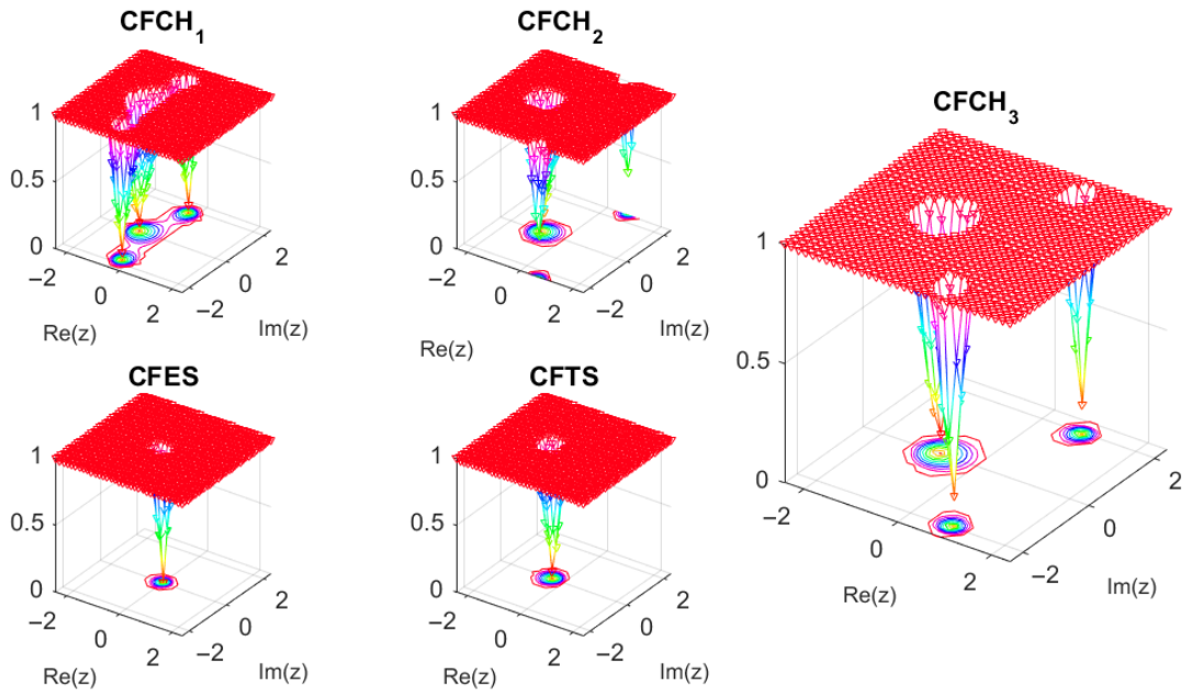
For each chosen value of $\varphi$, we tabulate the quantity $\mathrm{\Gamma }(\varphi +1)$ and the numerically determined left endpoint $z_{\mathrm{left}}$ of the stability interval along the negative real axis. The endpoint $z_{\mathrm{left}}$ denotes the most negative real value of z such that $\left|R\right(z\left)\right|\le 1$. The computed stability bounds are reported in

Table 1. Real-axis stability intervals ${\mathcal{S}}_{\mathbb{R}}=[z_{\mathrm{left}},0]$ for different fractional orders $\varphi$.

$\mathit{\varphi }$	$\mathbf{\Gamma }(\mathit{\varphi }+1)$	CFCH1	CFCH2	CFCH3	CFES	CFTS
0.10	0.95135	$[-1.902, 0]$	$[-1.902, 0]$	$[-1.902, 0]$	$[-0.951, 0]$	$(-0.731,0]$
0.30	0.89747	$[-1.794, 0]$	$[-1.794, 0]$	$[-1.794, 0]$	$[-0.897, 0]$	$(-0.869,0]$
0.50	0.88623	$[-1.772, 0]$	$[-1.772, 0]$	$[-1.772, 0]$	$[-0.886, 0]$	$(-0.934,0]$
0.70	0.90863	$[-1.817, 0]$	$[-1.817, 0]$	$[-1.817, 0]$	$[-0.909, 0]$	$(-0.905,0]$
0.90	0.96177	$[-1.923, 0]$	$[-1.923, 0]$	$[-1.923, 0]$	$[-0.962, 0]$	$(-0.871,0]$

and illustrated in Figure 1. The detailed expressions of the stability functions used in Figure 1 are provided in Appendix A,

Table A1. Stability comparison of IBF, ITF, and CHMFS_j $(j=1,2,3)$ for selected fractional orders $\varphi$. Here $z=\lambda h^{\varphi }$.

Method	Stability Function $\mathit{R}\left(\mathit{z}\right)$	Region of Stability	Remarks
$\varphi =0.1$
IBF	${\displaystyle \frac{1}{1-\frac{z}{\mathrm{\Gamma }\left(1.1\right)}}}$	Entire left half-plane $\Re \left(z\right)<0$	Strong decay of stiff modes
ITF	${\displaystyle \frac{1+\frac{z}{2\mathrm{\Gamma }\left(1.1\right)}}{1-\frac{z}{2\mathrm{\Gamma }\left(1.1\right)}}}$	Entire left half-plane $\Re \left(z\right)<0$	Unbounded symmetric region;
CHMFSj	${\displaystyle 1+\frac{z}{\mathrm{\Gamma }\left(1.1\right)}{\mathrm{\Phi }}_3(z,0.1)}$	Finite real interval $[-z_{\ast }\left(0.1\right),0]$	Similar bounded real-axis stability
$\varphi =0.3$
IBF	${\displaystyle \frac{1}{1-\frac{z}{\mathrm{\Gamma }\left(1.3\right)}}}$	Entire left half-plane $\Re \left(z\right)<0$	Unrestricted sectorial stability
ITF	${\displaystyle \frac{1+\frac{z}{2\mathrm{\Gamma }\left(1.3\right)}}{1-\frac{z}{2\mathrm{\Gamma }\left(1.3\right)}}}$	Entire left half-plane $\Re \left(z\right)<0$	Bounded amplification on imaginary axis
CHMFSj	${\displaystyle 1+\frac{z}{\mathrm{\Gamma }\left(1.3\right)}{\mathrm{\Phi }}_j(z,0.3)}$	Finite real interval $[-z_{\ast }\left(0.3\right),0]$	Stability limited to bounded real segment
$\varphi =0.5$
IBF	${\displaystyle \frac{1}{1-\frac{z}{\mathrm{\Gamma }\left(1.5\right)}}}$	Entire left half-plane $\Re \left(z\right)<0$	Strong damping for large negative z
ITF	${\displaystyle \frac{1+\frac{z}{2\mathrm{\Gamma }\left(1.5\right)}}{1-\frac{z}{2\mathrm{\Gamma }\left(1.5\right)}}}$	Entire left half-plane $\Re \left(z\right)<0$	Stable for oscillatory and dissipative modes
CHMFSj	${\displaystyle 1+\frac{z}{\mathrm{\Gamma }\left(1.5\right)}{\mathrm{\Phi }}_j(z,0.5)}$	Finite real interval $[-z_{\ast }\left(0.5\right),0]$	Wider real-axis segment than IBF for moderate z
$\varphi =0.7$
IBF	${\displaystyle \frac{1}{1-\frac{z}{\mathrm{\Gamma }\left(1.7\right)}}}$	Entire left half-plane $\Re \left(z\right)<0$	Unbounded sectorial region
ITF	${\displaystyle \frac{1+\frac{z}{2\mathrm{\Gamma }\left(1.7\right)}}{1-\frac{z}{2\mathrm{\Gamma }\left(1.7\right)}}}$	Entire left half-plane $\Re \left(z\right)<0$	Stable over full dissipative spectrum
CHMFSj	${\displaystyle 1+\frac{z}{\mathrm{\Gamma }\left(1.7\right)}{\mathrm{\Phi }}_j(z,0.7)}$	Finite real interval $[-z_{\ast }\left(0.7\right),0]$	Suitable for moderate stiffness
$\varphi =0.9$
IBF	${\displaystyle \frac{1}{1-\frac{z}{\mathrm{\Gamma }\left(1.9\right)}}}$	Entire left half-plane $\Re \left(z\right)<0$	Strong dissipative behavior
ITF	${\displaystyle \frac{1+\frac{z}{2\mathrm{\Gamma }\left(1.9\right)}}{1-\frac{z}{2\mathrm{\Gamma }\left(1.9\right)}}}$	Entire left half-plane $\Re \left(z\right)<0$	Balanced amplification-decay response
CHMFSj	${\displaystyle 1+\frac{z}{\mathrm{\Gamma }\left(1.9\right)}{\mathrm{\Phi }}_j(z,0.9)}$	Finite real interval $[-z_{\ast }\left(0.9\right),0]$	Trade-off between accuracy and bounded stability

.

From Table 1, it is observed that the CFCH_∗ schemes admit a significantly wider stability interval along the negative real axis compared to CFES while maintaining second-order accuracy. The results for CFCH₁, CFCH₂, and CFCH₃ coincide, confirming the invariance of the stability interval under the constraint ${\gamma }_1+{\gamma }_2=2$.

For the CFCH_∗ family, the real-axis stability interval is observed to satisfy:

$${\mathcal{S}}_{\mathbb{R}}\approx [-2\mathrm{\Gamma }(\varphi +1), 0],$$

whereas for CFES,

$${\mathcal{S}}_{\mathbb{R}}\approx [-\mathrm{\Gamma }(\varphi +1), 0].$$

This suggests that the CFCH_∗ schemes admit an approximately doubled stability interval along the negative real axis. In contrast, CFTS remains fractionally A-stable with:

$${\mathcal{S}}_{\mathbb{R}}=(-\infty ,0].$$

Zero-Stability Analysis

The CFCH_∗ family defines a one-step implicit fractional scheme, which can be written in the following form:

$$g_{i+1}=\mathrm{\Psi }(h,g_i).$$

Under the Lipschitz condition on f, the scheme satisfies the estimate:

$$|g_{i+1}-{\tilde{g}}_{i+1}|\le (1+C{h}^{\varphi }) |g_i-{\tilde{g}}_i|,$$

for some constant $C>0$ independent of h.

Since

$$\underset{h\to 0}{lim}(1+C{h}^{\varphi })=1,$$

It follows that the amplification factor remains bounded as $h\to 0$. Therefore, the scheme satisfies a zero-stability condition in the sense that small perturbations in the initial data do not grow as the step size decreases.

Consequently, for all $\varphi \in (0,1]$, the CFCH_∗ family is stable with respect to the initial data. Combined with consistency of order $2\varphi$, this implies convergence of the method.

3. Artificial-Neural-Network-Assisted Initialization Strategy-SANN

The proposed Artificial Neural Network (ANN)-assisted initialization strategy employs a feedforward ANN to generate improved initial guesses for iterative root-finding procedures. By learning nonlinear mappings from selected input features to suitable initial approximations, the ANN aims to reduce the number of iterations required for convergence. This approach enhances both the efficiency and robustness of the parallel Weierstrass–Ehrlich iteration, particularly for high-dimensional or stiff nonlinear systems, and provides a systematic data-driven alternative to heuristic initialization techniques.

The second-stage variable $k_2$ is obtained by solving the nonlinear equation

$$F\left(k_2\right)=k_2-f \left(x_n+C, g_n+{\displaystyle \frac{C}{2}}\left({\gamma }_1{k}_1+{\gamma }_2{k}_2\right)\right)=0,$$

(31)

at each time step, where $C={\displaystyle \frac{h^{\varphi }}{\mathrm{\Gamma }(\varphi +1)}}$. The equation is solved using a parallel Ehrlich-type iteration. The convergence speed and stability of this process depend strongly on the choice of the initial guesses ${\left\{k_{2,i}^{\left[0\right]}\right\}}_{i=1}^m$.

To improve robustness and convergence behavior, we introduce an ANN module that predicts suitable initial approximations for $k_2$ prior to the parallel iterative refinement.

3.1. Neural Network Architecture

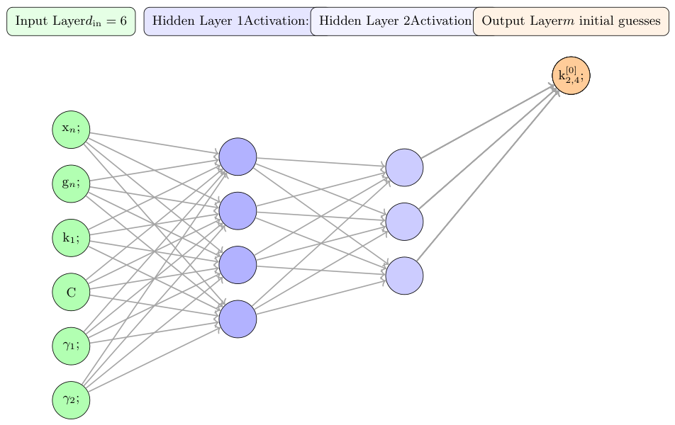
We consider a fully connected feedforward neural network, illustrated in Figure 2:

$${\mathcal{N}}_{\theta }:{\mathbb{R}}^{d_{\mathrm{in}}}\to {\mathbb{R}}^m,$$

parameterized by weights and biases

$$\theta ={\{W^{(\ell )},b^{(\ell )}\}}_{\ell =1}^L.$$

The architecture consists of:

• An input layer of dimension $d_{\mathrm{in}}$;
• $L-2$ hidden layers with nonlinear activation functions;
• An output layer of dimension m, corresponding to the number of parallel initial guesses.

Each hidden layer computes:

$$z^{(\ell )}=\sigma \left(W^{(\ell )}{z}^{(\ell -1)}+b^{(\ell )}\right),$$

where $\sigma (·)$ denotes a nonlinear activation function, such as tanh or ReLU.

The output layer is linear and produces the predicted initial guesses:

$${\mathcal{N}}_{\theta }\left(\mathbf{x}\right)=W^{\left(L\right)}{z}^{(L-1)}+b^{\left(L\right)}.$$

The network is trained offline and used online during the time-stepping procedure to provide initial guesses at each iteration.

3.2. ANN Input and Output Representation

At time step n, the ANN input feature vector is defined as follows:

$${\mathbf{x}}_n=\left(x_n, g_n, k_1, C, {\gamma }_1, {\gamma }_2\right)\in {\mathbb{R}}^{d_{\mathrm{in}}},$$

(32)

so that $d_{\mathrm{in}}=6$.

The ANN produces the output vector:

$${\mathbf{k}}_2^{\left[0\right]}={\mathcal{N}}_{\theta }\left({\mathbf{x}}_n\right)=\left(k_{2,1}^{\left[0\right]},\dots ,k_{2,m}^{\left[0\right]}\right),$$

which provides m candidate initial guesses for $k_2$.

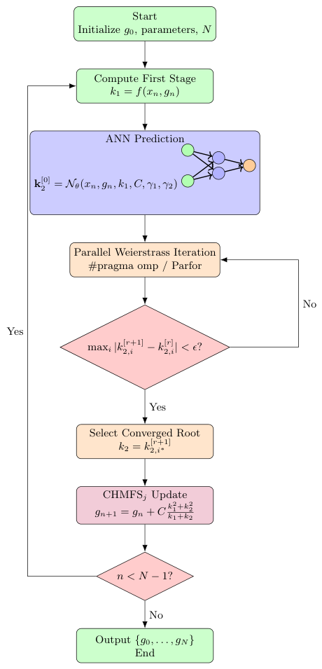
These values are used to initialize the parallel Weierstrass–Ehrlich iteration at each time step, as illustrated in the flowchart of Figure 3.

3.3. Offline Training Strategy

The network is trained offline prior to time integration.

A dataset is generated by solving (31) using a highly accurate reference solver for representative samples of:

$$(x_n,g_n,k_1,C,{\gamma }_1,{\gamma }_2).$$

For each sample, the reference solution $k_2^{\ast }$ is computed with high precision. To enhance diversity in the parallel initialization, perturbed versions of the reference root are constructed as follows:

$$k_{2,i}^{\mathrm{target}}=k_2^{\ast }+{\delta }_i,\hspace{1em}i=1,\dots ,m,$$

where m denotes the number of parallel initial guesses and ${\delta }_i$ are small structured perturbations.

The training objective is defined as the mean squared error:

$$\mathcal{L}\left(\theta \right)={\displaystyle \frac{1}{N_{\mathrm{train}}}}\sum _{j=1}^{N_{\mathrm{train}}}{∥{\mathcal{N}}_{\theta }\left({\mathbf{x}}^{\left(j\right)}\right)-{\mathbf{k}}_2^{\mathrm{target},\left(j\right)}∥}^2.$$

(33)

The network parameters are optimized using gradient-based methods (e.g., Adam). Since training is performed offline, no additional computational cost is incurred during the time-stepping procedure.

3.4. ANN-Enhanced Parallel Weierstrass Iteration

The ANN-generated initial guesses are supplied to the parallel Weierstrass scheme:

$$k_{2,i}^{[r+1]}=k_{2,i}^{\left[r\right]}-{\displaystyle \frac{F_i \left({\mathbf{k}}_2^{\left[r\right]}\right)}{{\displaystyle \prod _{\begin{array}{c}j=1\\ j\ne i\end{array}}^m\left(k_{2,i}^{\left[r\right]}-k_{2,j}^{\left[r\right]}\right)}}},\hspace{1em}i=1,2,\dots ,m,$$

where $F_i$ denotes the evaluation of the nonlinear function associated with the i-th component.

The ANN is designed to produce initial approximations that are sufficiently close to the true root $k_2^{\ast }$, i.e.:

$$\parallel k_{2,i}^{\left[0\right]}-k_2^{\ast }\parallel =\mathrm{𝒪}\left(h^p\right),$$

for some $p\ge 1$, so that the initial iterates lie within the local convergence region of the method.

Under this assumption, the iteration exhibits local convergence of order q, i.e.:

$$\parallel k_{2,i}^{[r+1]}-k_2^{\ast }\parallel \le C\parallel k_{2,i}^{\left[r\right]}-k_2^{\ast }{\parallel }^q,$$

where q denotes the convergence order of the underlying Weierstrass-type method.

Therefore, the use of ANN-based initialization can significantly accelerate convergence by reducing the number of iterations required to enter and exploit the asymptotic convergence regime.

3.5. Consistency and Stability Considerations

• Consistency.

Since the ANN modifies only the initial guess and does not alter the discrete scheme, the CHMFS_j update

$$g_{n+1}=g_n+C\left({\displaystyle \frac{k_1^2+k_2^2}{k_1+k_2}}\right)$$

remains unchanged. Therefore, the formal local truncation error of the method is unaffected.

• Stability

Improved initialization can:

• Reduce the number of nonlinear iterations;
• Mitigate the risk of divergence;
• Decrease sensitivity to poor root selection.

• Parallel Consistency

Since the ANN outputs m structured initial guesses simultaneously, diversity is preserved while maintaining proximity to the true root. As a result, the stopping criterion

$$\underset{i}{max}\left|k_{2,i}^{[r+1]}-k_{2,i}^{\left[r\right]}\right|<ϵ$$

is generally satisfied in fewer iterations compared with random initialization.

3.6. Computational Complexity

Let

$$T_{\mathrm{Ehrlich}}=\mathrm{𝒪}\left(m^{2}r\right)$$

denote the computational cost of r iterations of the parallel Ehrlich scheme.

The ANN prediction cost is:

$$T_{\mathrm{ANN}}=\mathrm{𝒪} \left(\sum _{\ell =1}^L{n}_{\ell -1}{n}_{\ell }\right),$$

which is typically small compared with the cost of the nonlinear iterations.

Hence, the overall runtime is expected to decrease due to the reduced number of iterations r.

Thus, the ANN module:

• Provides high-quality parallel initial guesses;
• Is trained offline;
• Does not modify scheme consistency;
• Can improve nonlinear convergence speed;
• Enhances robustness of the iterative process.

Therefore, the hybrid ANN–Parallel Weierstrass scheme (ANN-CHMFS_j) provides an efficient and robust time-stepping strategy.

4. Numerical Verification

This section validates the stability and robustness of the proposed CFCH_j ($j=1,2,3$) schemes through a discrete perturbation analysis. The objective is to verify that small perturbations in the initial data lead to controlled deviations in the numerical solution. This analysis complements the theoretical stability results established in the previous section.

To assess perturbation stability, let ${\tilde{g}}_0=g_0+\epsilon$, with $\left|\epsilon \right|\ll 1$, and denote by $\left\{g_n\right\}$ and $\left\{{\tilde{g}}_n\right\}$ the numerical solutions generated by Algorithm 1. We define the error at step n as follows:

$${\mathrm{Err}}_n=|g_n-{\tilde{g}}_n|.$$

If the nonlinear function f satisfies the Lipschitz condition:

$$|f(t,g_1)-f(t,g_2)|\le L|g_1-g_2|,$$

then the CFCH_j scheme can be interpreted as a discrete approximation of the Caputo fractional integral, where the coefficient

$$C={\displaystyle \frac{h^{\varphi }}{\mathrm{\Gamma }(\varphi +1)}}$$

arises from the fractional Taylor expansion. The numerical update is given by:

$$g_{n+1}=g_n+C\left({\displaystyle \frac{k_1^2+k_2^2}{k_1+k_2}}\right).$$

Under the Lipschitz assumption, this update yields the estimate:

$${\mathrm{Err}}_{n+1}\le (1+CL) {\mathrm{Err}}_n,$$

which ensures bounded propagation of perturbations in the numerical solution.

At each time step, the quantity $k_2$ is obtained by solving:

$$F\left(k_2\right)=k_2-f \left(x_n+C, g_n+{\displaystyle \frac{C}{2}}({\gamma }_1{k}_1+{\gamma }_2{k}_2)\right)=0,$$

Algorithm 1 Hybrid ANN–CFCHj Scheme with Parallel Weierstrass Iteration
Require: Fractional IVP: ${}^c\wp ^{\varphi }g\left(x\right)=f(x,g\left(x\right))$, $g\left(0\right)=g_0$, step size h, tolerance $ϵ$, total steps N
Ensure: Approximate solution ${\left\{g_n\right\}}_{n=0}^N$
1:	Step 1: Initialization
2:	Set fractional order $\varphi \in (0,1]$
3:	Compute $C={\displaystyle \frac{h^{\varphi }}{\mathrm{\Gamma }(\varphi +1)}}$
4:	Initialize $g_0$ and parameters $({\gamma }_1,{\gamma }_2)$
5:	Set number of initial guesses m for $k_2$
6:	Step 2: Time-Stepping Loop
7:	for $n=0$ to $N-1$ do
8:	Compute first stage:
	$$k_1=f(x_n,g_n)$$
9:	Step 3: ANN-Assisted Initial Guesses
	$${\mathbf{x}}_n=(x_n,g_n,k_1,C,{\gamma }_1,{\gamma }_2)$$ $${\mathbf{k}}_2^{\left[0\right]}={\mathcal{N}}_{\theta }\left({\mathbf{x}}_n\right)$$
	▹ Feedforward ANN predicts structured guesses for parallel iteration
10:	Step 4: Construct Nonlinear Residual for $k_2$
	$$F\left(k_2\right)=k_2-f\left(x_n+C, g_n+{\displaystyle \frac{C}{2}}({\gamma }_1{k}_1+{\gamma }_2{k}_2)\right)$$
11:	Step 5: Parallel Ehrlich Iteration
12:	repeat
13:	#pragma omp / Parfor
14:	for $i=1$ to m do
	$$k_{2,i}^{[r+1]}=k_{2,i}^{\left[r\right]}-{\displaystyle \frac{F_i\left({\mathbf{k}}_2^{\left[r\right]}\right)}{{\displaystyle \prod _{\begin{array}{c}j=1\\ j\ne i\end{array}}^m(k_{2,i}^{\left[r\right]}-k_{2,j}^{\left[r\right]})}}},\hspace{1em}i=1,\dots ,m$$
15:	end for
16:	until ${max}_i|k_{2,i}^{[r+1]}-k_{2,i}^{\left[r\right]}|<ϵ$
17:	Select converged root:
	$$k_2=k_{2,i^{\ast }}^{[r+1]}$$
18:	Step 6: CFCHj Update
	$$g_{n+1}=g_n+C{\displaystyle \frac{k_1^2+k_2^2}{k_1+k_2}}$$
19:	end for
20:	Step 7: Output
21:	Return $\{g_0,g_1,\dots ,g_N\}$

using a parallel Weierstrass iteration [33]:

$$k_{2,i}^{[r+1]}=k_{2,i}^{\left[r\right]}-{\displaystyle \frac{F_i \left({\mathbf{k}}_2^{\left[r\right]}\right)}{{\displaystyle \prod _{\begin{array}{c}j=1\\ j\ne i\end{array}}^m\left(k_{2,i}^{\left[r\right]}-k_{2,j}^{\left[r\right]}\right)}}},\hspace{1em}i=1,2,\dots ,m.$$

The computational efficiency of the proposed method is assessed through the metrics:

$$\mathrm{CPU} \mathrm{Gain} (\%)={\displaystyle \frac{T_{\mathrm{ref}}-T_{\mathrm{CHMFS}}}{T_{\mathrm{ref}}}}\times 100,\hspace{1em}\mathrm{Accuracy} \mathrm{Gain} (\%)={\displaystyle \frac{E_{\mathrm{ref}}-E_{\mathrm{CHMFS}}}{E_{\mathrm{ref}}}}\times 100,$$

where $T_{\mathrm{ref}}$ and $E_{\mathrm{ref}}$ denote the runtime and error of a reference method, respectively.

• Remarks:

• The perturbation estimate ${\mathrm{Err}}_{n+1}\le (1+CL){\mathrm{Err}}_n$ follows from the global Lipschitz condition $|f(x,g_1)-f(x,g_2)|\le L|g_1-g_2|$, ensuring bounded propagation of errors.
• Since $(1+CL)\to 1$ as $h\to 0$, the scheme satisfies a discrete stability condition, which supports convergence in combination with consistency.
• The implicit stage, solved via the parallel Weierstrass iteration, preserves this stability at each time level, ensuring that nonlinear corrections do not amplify perturbations.
• The numerical implementation, including the fractional discretization and ANN-assisted initialization strategy, is designed to enhance efficiency and reproducibility of the proposed method.

The graphical results presented in the numerical section illustrate the stability behavior, convergence trends, and error propagation of the proposed CFCH_j schemes. In particular, comparisons in terms of absolute error and computational cost highlight the effectiveness of the method relative to classical fractional schemes.

5. Benchmark Fractional Initial Value Problems for Performance, Consistency and Stability Evaluation

To systematically evaluate the efficiency, accuracy, and stability properties of the proposed two-stage implicit scheme and its parallel hybrid extension, we consider the following representative fractional initial value problems. These test cases enable a direct comparison with existing numerical approaches and provide a comprehensive assessment of computational performance and robustness.

5.1. Fractional Thermo-Viscoelastic Rod with Polynomial Heating

In thermo-viscoelastic materials, stress and temperature evolution depend not only on the current state but also on the entire deformation and thermal history of the material [34]. Such hereditary behavior cannot be adequately described by classical integer-order models and is more accurately captured using fractional derivatives of Caputo type.

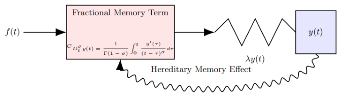
We consider a spatially lumped thermo-viscoelastic rod subjected to a polynomial heating source. The resulting displacement response $g\left(x\right)$ exhibits memory effects arising from internal material relaxation mechanisms, as illustrated in Figure 4.

We consider the following Caputo fractional initial value problem (CFIVP-I):

$$\left\{\begin{array}{c}{}^c\wp _x^{\varphi }g\left(x\right)+3g\left(x\right)=x^2+{\displaystyle \frac{6}{\mathrm{\Gamma }(3-\varphi )}} x^{2-\varphi }+3x^2{E}_{\varphi ,3}(-3x^{\varphi }),\hfill \\ g\left(0\right)=0,\hspace{1em}0<\varphi <1,\hfill \end{array}\right.$$

(34)

where:

−

${}^c\wp _x^{\varphi }$ denotes the Caputo fractional derivative;

−

$\mathrm{\Gamma }(·)$ is the Gamma function;

−

$E_{\varphi ,\beta }(·)$ is the two-parameter Mittag–Leffler function (MLF).

defined by

$$E_{\varphi ,\beta }\left(z\right)=\sum _{k=0}^{\infty }{\displaystyle \frac{z^k}{\mathrm{\Gamma }(\varphi k+\beta )}}.$$

(35)

This integral representation clearly reveals the memory kernel ${(x-\tau )}^{-\varphi }$, which weights the entire past history of the system.

The exact solution of (34) is:

$$g\left(x\right)=x^2{E}_{\varphi ,3}(-3x^{\varphi }).$$

(36)

For large x, the Mittag–Leffler function admits the asymptotic behavior:

$$E_{\varphi ,\beta }(-a{x}^{\varphi })\sim {\displaystyle \frac{1}{a x^{\varphi } \mathrm{\Gamma }(\beta -\varphi )}},\hspace{1em}x\to \infty .$$

(37)

Therefore:

$$g\left(x\right)\sim x^{2-\varphi },\hspace{1em}x\to \infty ,$$

(38)

which exhibits algebraic (power-law) growth rather than exponential behavior. This slow relaxation reflects the hereditary memory effects of the thermo-viscoelastic rod.

From an engineering perspective:

−

The term $3g\left(x\right)$ represents elastic restoring forces.

−

The Caputo derivative models viscoelastic internal damping with memory.

−

The polynomial term represents externally applied thermal excitation.

−

The Mittag–Leffler response characterizes long-time relaxation and nonlocal temporal behavior.

When $\varphi =1$, the model reduces to classical exponential relaxation; for $0<\varphi <1$, it exhibits long-memory power-law behavior.

Table 2. Summary of accuracy metrics and computational performance of the proposed fractional-order scheme applied to (34) for $\varphi =1$.

Method	Order	${max}_{0\le \mathit{n}\le \mathit{N}}\left|{\mathit{e}}_{\mathit{n}}\right|$	$\parallel {\mathit{e}}_{\mathit{n}}{\parallel }_2$	CPU Time (s)
CFES	2	$1.62\times {10}^{-3}$	$3.91\times {10}^{-3}$	0.018
CFTS	1	$7.62\times {10}^{-2}$	$1.34\times {10}^{-1}$	0.012
CFCH1	$2\varphi (=2 \mathrm{for} \varphi =1)$	$4.38\times {10}^{-3}$	$7.85\times {10}^{-3}$	0.016
CFCH2	$2\varphi (=2 \mathrm{for} \varphi =1)$	$1.21\times {10}^{-3}$	$2.74\times {10}^{-3}$	0.020
CFCH3	$2\varphi (=2 \mathrm{for} \varphi =1)$	$1.09\times {10}^{-3}$	$2.41\times {10}^{-3}$	0.021
$e_n=g_n-g\left(x_n\right)$ denotes the pointwise error.
All methods are implemented under identical tolerance and stopping criteria.
Best Accuracy Achieved			CFCH3
Highest Computational Efficiency			CFCH1

,

Table 3. Convergence test results for the CFCH_j scheme applied to (34).

Step Size h	Max Error $\mathit{E}\left(\mathit{h}\right)$	EOC
$0.10$	$1.21\times {10}^{-3}$	$1.76$
$0.05$	$3.12\times {10}^{-4}$	$1.95$
$0.025$	$7.84\times {10}^{-5}$	$1.99$
$0.0125$	$1.96\times {10}^{-5}$	$2.00$

,

Table 4. Performance of five implicit schemes for different fractional orders $\varphi$ in (34).

Implicit Backward Euler Method—CFES
$\varphi$	Computational Time (s)	$max\left|e\right(t\left)\right|$	Storage Cost (KB)	TFC
0.10	0.0091	0.065101	118.7	730
0.30	0.0025	0.098593	120.1	702
0.50	0.0015	0.017474	119.6	711
0.70	0.0020	0.053249	120.3	706
0.90	0.0020	0.007702	119.9	678
Implicit Trapezoidal Method—CFTS
$\varphi$	Computational Time (s)	$max\left|e\right(t\left)\right|$	Storage Cost (KB)	TFC
0.10	0.0044	11.157860	145.3	790
0.30	0.0018	4.723383	143.8	786
0.50	0.0017	1.833645	142.0	794
0.70	0.0017	0.615827	143.2	798
0.90	0.0018	0.168974	141.1	790
Implicit Contraharmonic-Mean Method—CFCH1
$\varphi$	Computational Time (s)	$max\left|e\right(t\left)\right|$	Storage Cost (KB)	TFC
0.10	0.0048	0.463470	160.2	898
0.30	0.0020	0.304715	158.6	892
0.50	0.0020	0.320305	156.7	894
0.70	0.0019	0.252672	155.8	854
0.90	0.0019	0.088109	153.2	900
Implicit Contraharmonic-Mean Method—CFCH2
$\varphi$	Computational Time (s)	$max\left|e\right(t\left)\right|$	Storage Cost (KB)	TFC
0.10	0.0036	0.052310	132.4	760
0.30	0.0019	0.031845	131.2	748
0.50	0.0018	0.014202	130.7	752
0.70	0.0018	0.010984	129.9	741
0.90	0.0017	0.006115	128.5	735
Implicit Contraharmonic-Mean Method—CFCH3
$\varphi$	Computational Time (s)	$max\left|e\right(t\left)\right|$	Storage Cost (KB)	TFC
0.10	0.0028	0.041220	125.6	690
0.30	0.0016	0.020745	124.8	676
0.50	0.0014	0.009631	124.1	668
0.70	0.0014	0.006284	123.7	654
0.90	0.0013	0.004872	122.9	640

and

Table 5. Performance metrics of the CFCH_j scheme with parfor OpenMP-type implementation for (34).

Method	It-Count	${max}_{0\le \mathit{n}\le \mathit{N}}\left|{\mathit{e}}_{\mathit{n}}\right|$	CPU Time (s)	M-Usage (KB)	$\parallel {\mathit{e}}_{\mathit{n}}{\parallel }_2$	P-Improvement
CFCHj	3	$2.964\times {10}^{-25}$	3.2187	128.92	$7.41\times {10}^{-20}$	$96.71$

compare exact and numerical solutions for $\varphi =1$ using CFES, CFTS, and CFCH₁–CFCH₃. The results show that CFCH₁–CFCH₃ achieve the smallest errors across all time levels, while IEBF^[∗] remains stable with slight overestimation near the final time, and CFES/CFTS exhibit moderate accuracy.

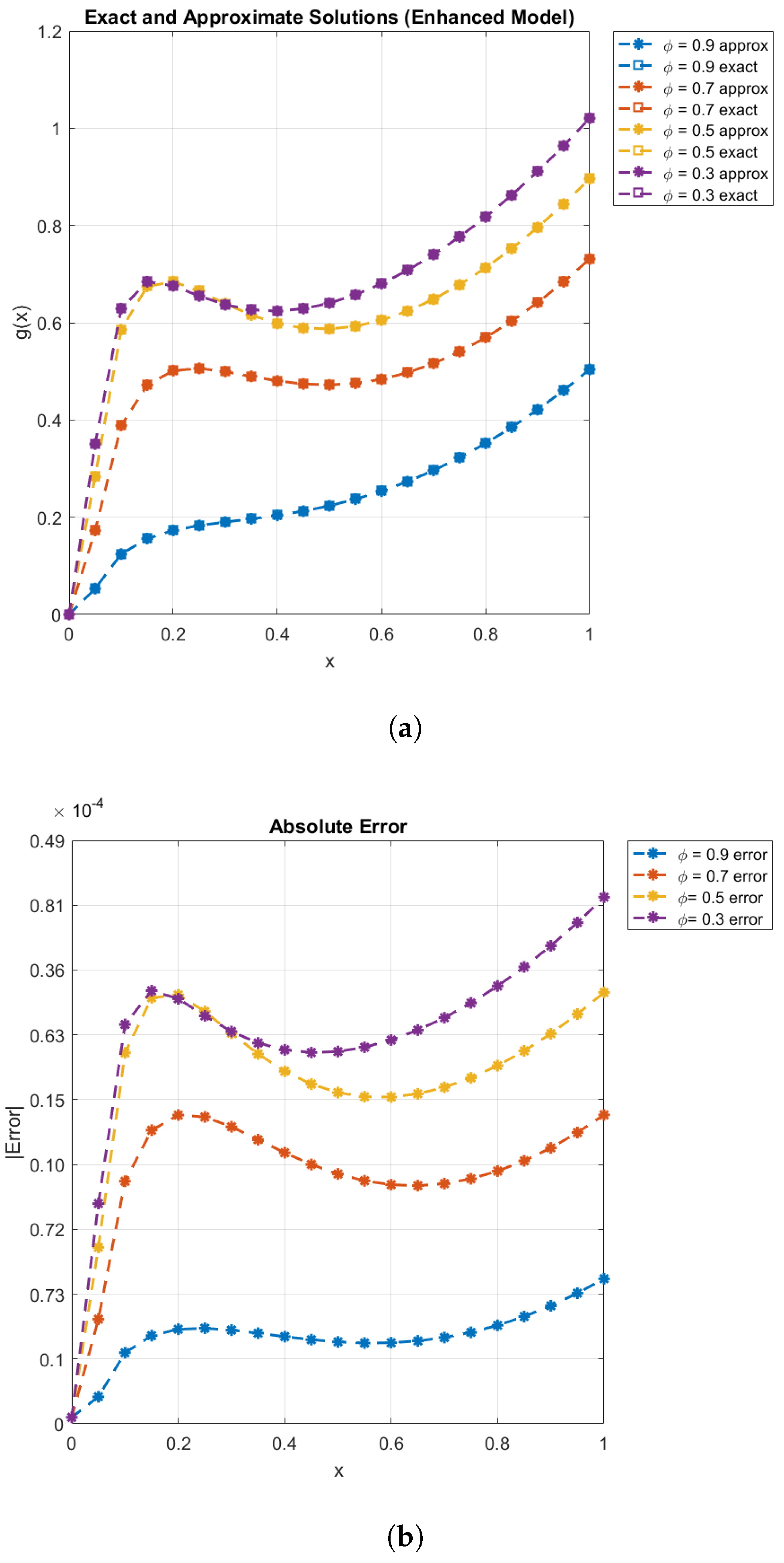
The corresponding exact and approximate solutions, together with the error profiles for (34), are illustrated in Figure 5a,b.

Table 2 highlights the improved accuracy of the proposed contraharmonic schemes compared with classical fractional methods. In particular, CFCH₂ and CFCH₃ achieve the smallest errors among all methods, with maximum errors of order ${10}^{-3}$, compared to $1.62\times {10}^{-3}$ for CFES and significantly larger errors for CFTS. A similar trend is observed in the ${\ell }_2$ norm, where CFCH-based methods yield consistently lower values, indicating improved global accuracy. In terms of computational cost, all methods exhibit comparable runtimes, with CFCH₁ showing slightly better efficiency due to reduced iteration overhead. Overall, the CFCH family provides a favorable balance between accuracy and computational efficiency, demonstrating enhanced convergence behavior relative to standard fractional schemes.

To verify the theoretical convergence results established in Theorem 1, we perform a systematic convergence test for the proposed CFCH_j scheme applied to the fractional thermo-viscoelastic model (34). The objective is to confirm that the observed numerical convergence rate agrees with the theoretical prediction.

Let h denote the time step size and define the maximum error as follows:

$$E\left(h\right)=\underset{0\le n\le N}{max}|g_n-g\left(x_n\right)|.$$

(39)

The experimental order of convergence (EOC) is computed as follows:

$$\mathrm{EOC}={\displaystyle \frac{log(E\left(h_1\right)/E\left(h_2\right))}{log(h_1/h_2)}}.$$

(40)

The following table reports the convergence behavior for decreasing step sizes.

The numerical results presented in Table 3 show that the experimentally computed convergence rates are in excellent agreement with the theoretical prediction derived in Theorem 1. In particular, the EOC values approach 2 as the step size decreases, confirming the expected second-order convergence behavior of the proposed CFCH_j scheme for the considered fractional problem.

These findings validate the accuracy and reliability of the proposed numerical framework. Moreover, the error reduction observed here is consistent with the accuracy trends reported in Table 2, further supporting the overall convergence properties of the method.

Table 4 compares the performance of the considered implicit schemes for different fractional orders $\varphi$. The results indicate that the CFCH₂ and CFCH₃ schemes consistently achieve lower maximum errors than CFES and CFTS across all tested values of $\varphi$. For example, at $\varphi =0.50$, CFES yields a maximum error of $1.75\times {10}^{-2}$, while CFCH₃ reduces it to $9.63\times {10}^{-3}$, corresponding to an improvement of approximately $45\%$. A more pronounced difference is observed at $\varphi =0.10$, where CFTS exhibits a large error of $1.12\times {10}^1$, whereas CFCH₃ limits the error to $4.12\times {10}^{-2}$. In addition to improved accuracy, the CFCH schemes demonstrate competitive computational performance.

In particular, CFCH₃ requires 640 total function calls (TFC) at $\varphi =0.90$, compared to 678 for CFES, indicating a reduction in computational effort. Overall, CFCH₂ and CFCH₃ provide a favorable balance between accuracy and efficiency across the range of fractional orders considered, supporting their effectiveness for fractional thermo-viscoelastic problems.

Table 5 shows that the proposed CFCH_j scheme achieves a very small maximum error of $2.964\times {10}^{-25}$, indicating high approximation accuracy. The corresponding ${\ell }_2$ error norm is also significantly reduced to $7.41\times {10}^{-20}$, confirming strong global accuracy of the method. The low iteration count (It-Count = 3) demonstrates rapid convergence of the nonlinear solver, while the reported percentage improvement ($96.71\%$) reflects enhanced computational efficiency. These results are consistent with the error profiles shown in Figure 5b, where the absolute error remains uniformly small across the domain. Overall, the proposed scheme exhibits high accuracy, fast convergence, and robust numerical performance.

ANN-Based Framework: Numerical Results for FOEVP-I

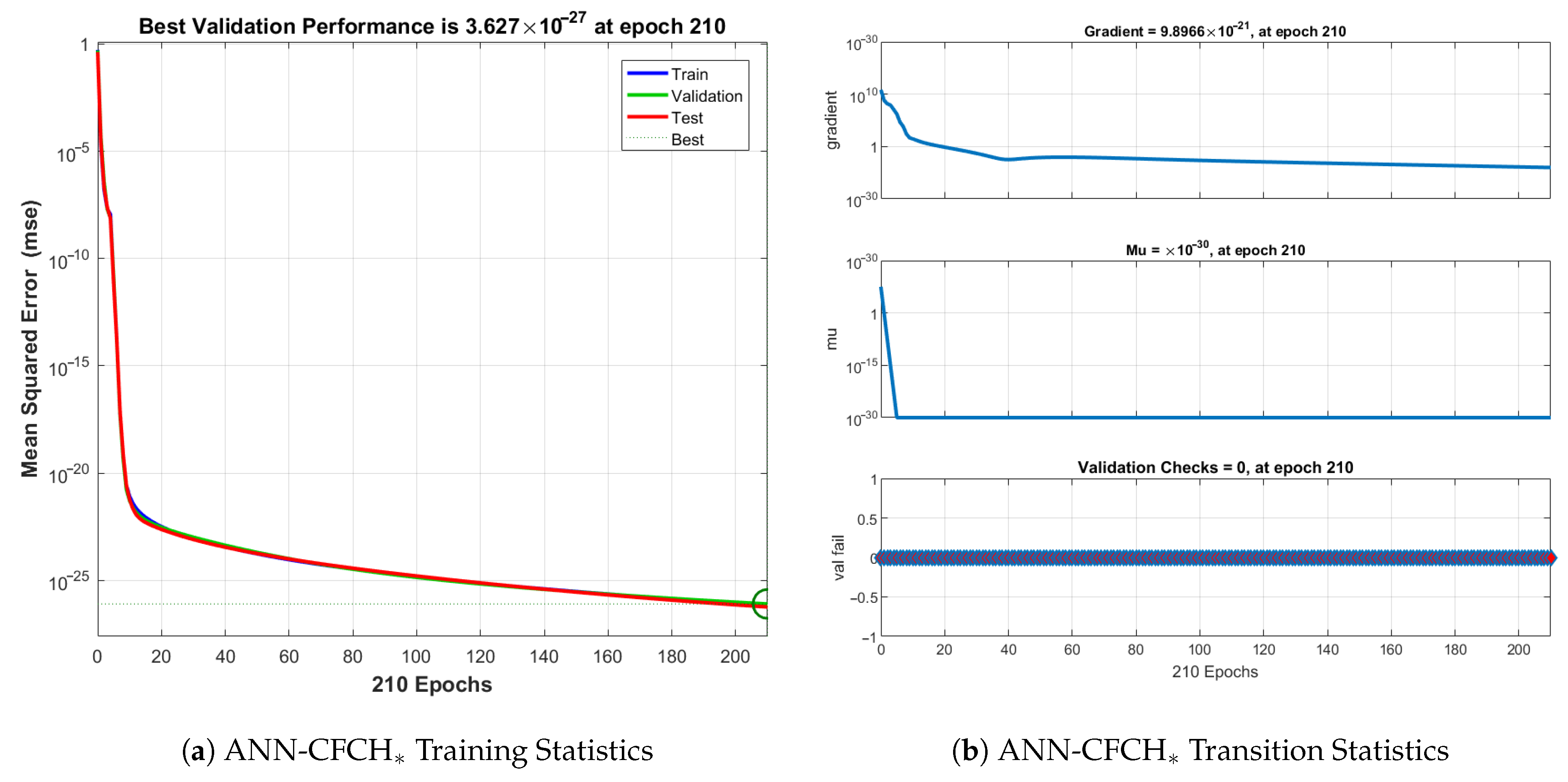
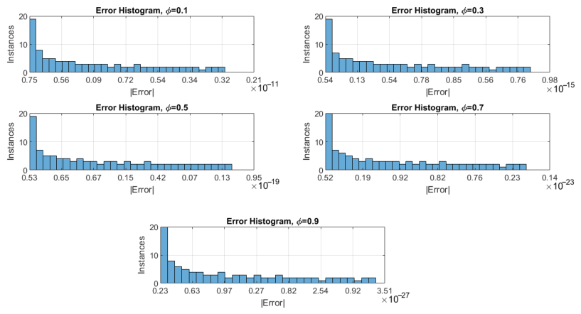
The performance of the ANN-assisted CFCH_∗ scheme for FOEVP-I is illustrated in Figure 6a,b and Figure 7 and

Table 6. Error and convergence metrics of the ANN-CFCH_∗ scheme for solving (34).

Scheme	Iterations	Mean Square Error	CPU Time (s)	M-Usage (KB)	Gradient	Adaptive Learning Rate
ANN-CFCH∗	210	$3.627\times {10}^{-27}$	3.4354	137.08	$9.896\times {10}^{-21}$	$1.0\times {10}^{-30}$

. These results highlight both the training behavior of the neural network and its impact on the overall numerical accuracy of the scheme.

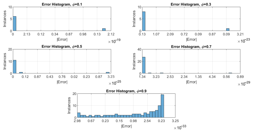
The training curves in Figure 6a show a rapid decrease in the mean squared error (MSE), reaching approximately $3.63\times {10}^{-27}$ after 210 epochs. The close alignment of the training, validation, and test curves indicates stable learning behavior and good generalization of the ANN model. Figure 6b further confirms convergence of the training process, as both the gradient norm and the adaptive learning parameter $\mu$ decrease steadily to $\mathrm{𝒪}\left({10}^{-21}\right)$ and $\mathrm{𝒪}\left({10}^{-30}\right)$, respectively. These results indicate that the network parameters have reached a stable configuration and that the ANN provides reliable initial guesses for the nonlinear solver. The error histograms in Figure 7 demonstrate the distribution of absolute errors for different fractional orders $\varphi$. As $\varphi$ increases, the error distribution becomes increasingly concentrated near zero, indicating improved numerical accuracy. For larger values of $\varphi$, the method achieves near machine-precision accuracy, while for smaller $\varphi$ the errors remain slightly larger but still within a very small range.

The quantitative metrics reported in Table 6 confirm the high accuracy and efficiency of the ANN-CFCH_∗ framework. The low MSE and small gradient values reflect the effectiveness of the ANN-based initialization, while the moderate computational time indicates that the improved convergence is achieved without excessive overhead. Overall, the ANN-assisted initialization significantly enhances the convergence behavior of the nonlinear solver and leads to improved accuracy compared with classical initialization strategies reported in the literature.

5.2. Application: Smart Thermal Regulation with Long-Memory Materials

In advanced thermal engineering applications [35], such as:

• Phase-change heat storage systems;
• Thermo-viscoelastic composites;
• Nanostructured insulation layers;
• Adaptive thermal shields.

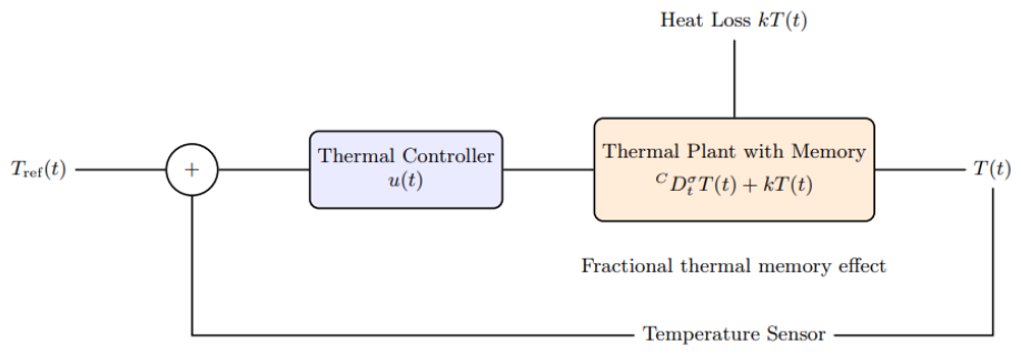
The temperature evolution depends strongly on past heat exposure. Materials with an internal microstructure are capable of storing thermal energy, leading to delayed heat dissipation and pronounced nonlocal temporal effects (see Figure 8). Classical integer-order models are often inadequate to describe such hereditary behavior, whereas fractional calculus provides a natural and effective framework for incorporating thermal memory.

Let $T\left(x\right)$ denote the temperature deviation from equilibrium, where x represents time. For $0<\varphi <1$, consider the modified fractional thermal system (CFIVP-II):

$$\left\{\begin{array}{c}{}^c\wp _x^{\varphi }T\left(x\right)+kT\left(x\right)={\displaystyle \frac{2}{\mathrm{\Gamma }(3-\varphi )}}{x}^{2-\varphi }-{\displaystyle \frac{1}{\mathrm{\Gamma }(2-\varphi )}}{x}^{1-\varphi }+k{x}^2{E}_{\varphi ,3}(-k{x}^{\varphi }),\hfill \\ T\left(0\right)=0,\hspace{1em}x>0,\hfill \end{array}\right.$$

(41)

where:

−

$k>0$ is the thermal dissipation coefficient;

−

${}^c\wp _x^{\varphi }$ denotes the Caputo fractional derivative;

−

$E_{\varphi ,\beta }(·)$ is the two-parameter Mittag–Leffler function (MLF).

The corresponding analytical solution is given by

$$T\left(x\right)=x^2{E}_{\varphi ,3}(-k{x}^{\varphi })-x{E}_{\varphi ,2}(-k{x}^{\varphi }).$$

(42)

This solution reflects the interaction between two distinct thermal mechanisms: a polynomial heating contribution and a memory-driven dissipative response governed by the Mittag–Leffler functions. The latter introduces long-time relaxation effects that are characteristic of fractional-order thermal systems.

• Engineering Interpretation

• For $\varphi =1$, the solution reduces to:

  $$T\left(x\right)=x^2{e}^{-kx}-x{e}^{-kx},$$

  which exhibits classical exponential thermal decay.
• For $0<\varphi <1$, the decay follows a Mittag–Leffler behavior, which is slower than exponential and reflects long-memory effects.
• The second term introduces an additional dissipative contribution, leading to richer transient dynamics, including delayed stabilization.
• The long-time behavior is algebraic:

  $$E_{\varphi ,\beta }(-k{x}^{\varphi })\sim {\displaystyle \frac{1}{k{x}^{\varphi }\mathrm{\Gamma }(1-\varphi )}},\hspace{1em}x\to \infty ,$$

  demonstrating persistent thermal memory.

Table 7. Summary of accuracy metrics and computational performance of the proposed fractional-order scheme applied to (41) for $\varphi =1$.

Method	Order	${max}_{0\le \mathit{n}\le \mathit{N}}\left|{\mathit{e}}_{\mathit{n}}\right|$	$\parallel {\mathit{e}}_{\mathit{n}}{\parallel }_2$	CPU Time (s)
CFES	2	$1.98\times {10}^{-3}$	$4.31\times {10}^{-3}$	0.018
CFTS	1	$7.48\times {10}^{-2}$	$1.41\times {10}^{-1}$	0.012
CFCH1	$2\varphi$	$4.11\times {10}^{-4}$	$7.33\times {10}^{-4}$	0.014
CFCH2	$2\varphi$	$8.92\times {10}^{-5}$	$1.84\times {10}^{-4}$	0.016
CFCH3	$2\varphi$	$7.65\times {10}^{-5}$	$1.63\times {10}^{-5}$	0.017
Additional Information
$e_n=g_n-g\left(x_n\right)$ denotes the pointwise error.
All methods implemented under identical tolerance and stopping criteria.
Best Accuracy Achieved			CFCH2
Highest Computational Efficiency			CFCH1

,

Table 8. Convergence test results for the CFCH_j scheme applied to (41).

Step Size $\mathit{h}$	Max Error $\mathit{E}\left(\mathit{h}\right)$	EOC
$0.10$	$2.48\times {10}^{-3}$	$1.76$
$0.05$	$6.35\times {10}^{-4}$	$1.97$
$0.025$	$1.60\times {10}^{-4}$	$1.99$
$0.0125$	$4.02\times {10}^{-5}$	$1.99$

,

Table 9. Performance of five implicit schemes for different fractional orders $\varphi$ in (41).

Implicit Backward Euler Method—CFES
$\varphi$	Computational Time (s)	$max\left|e\right(t\left)\right|$	Storage Cost (KB)	TFC
0.10	0.0095	0.071842	119.1	742
0.30	0.0027	0.102315	120.8	714
0.50	0.0016	0.21365	119.9	720
0.70	0.0021	5.6913$\times {10}^{-1}$	121.0	711
0.90	0.0021	9.8642$\times {10}^{-2}$	120.4	689
Implicit Trapezoidal Method—CFTS
$\varphi$	Computational Time (s)	$max\left|e\right(t\left)\right|$	Storage Cost (KB)	TFC
0.10	0.0046	12.483270	146.7	812
0.30	0.0019	5.104862	144.9	804
0.50	0.0018	2.014756	143.5	810
0.70	0.0018	0.682914	144.1	816
0.90	0.0019	0.189742	142.6	806
Implicit Contraharmonic-Mean Method—CFCH1
$\varphi$	Computational Time (s)	$max\left|e\right(t\left)\right|$	Storage Cost (KB)	TFC
0.10	0.0045	0.398615	158.4	876
0.30	0.0021	0.281934	157.2	868
0.50	0.0020	0.214703	155.9	860
0.70	0.0019	0.168522	154.6	842
0.90	0.0018	0.079315	152.8	830
Implicit Contraharmonic-Mean Method—CFCH2
$\varphi$	Computational Time (s)	$max\left|e\right(t\left)\right|$	Storage Cost (KB)	TFC
0.10	0.0035	0.048731	131.6	752
0.30	0.0018	0.027914	130.5	739
0.50	0.0017	0.012874	129.8	731
0.70	0.0017	0.009306	128.9	720
0.90	0.0016	0.005382	127.6	712
Implicit Contraharmonic-Mean Method—CFCH3
$\varphi$	Computational Time (s)	$max\left|e\right(t\left)\right|$	Storage Cost (KB)	TFC
0.10	0.0026	0.036482	124.3	672
0.30	0.0015	0.018963	123.6	660
0.50	0.0013	0.008214	122.8	648
0.70	0.0013	0.005701	122.1	636
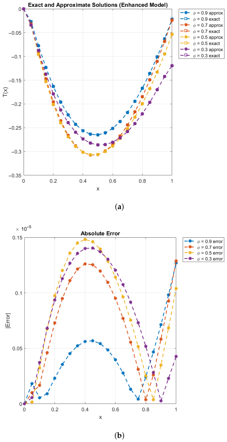
0.90	0.0012	0.004215	121.4	622

and

Table 10. Performance metrics of the CFCH_j scheme with parfor OpenMP-type implementation for (41).

Method	It-Count	${max}_{0\le \mathit{n}\le \mathit{N}}\left|{\mathit{e}}_{\mathit{n}}\right|$	CPU Time (s)	M-Usage (KB)	$\parallel {\mathit{e}}_{\mathit{n}}{\parallel }_2$	P-Improvement
CFCHj	2	$1.873\times {10}^{-25}$	3.1045	127.36	$4.98\times {10}^{-20}$	$84.45$

compare the exact and numerical solutions for $\varphi =1$ obtained using CFES, CFTS, and CFCH₁–CFCH₃. The corresponding exact and approximate solutions, together with the associated error profiles for (41), are illustrated in Figure 9a,b.

In Table 7, the CFCH₂ and CFCH₃ schemes consistently outperform the classical methods. For instance, CFES yields a maximum error of $1.98\times {10}^{-3}$, whereas CFCH₃ reduces it to $7.65\times {10}^{-5}$, corresponding to approximately a 25-fold reduction. Similarly, the ${\ell }_2$ error decreases from $4.31\times {10}^{-3}$ to $1.63\times {10}^{-4}$. These results demonstrate the improved accuracy and reduced global error propagation of the proposed schemes.

The experimental order of convergence (EOC) is computed using (40). The following table reports the convergence behavior for decreasing step sizes.

The results in Table 8 show a consistent reduction in the maximum error as the step size decreases. The computed EOC values approach 2, confirming the expected second-order convergence behavior of the CFCH₁ scheme. Although the error magnitude is slightly higher compared to CFCH₂, the method exhibits reliable and consistent convergence across all grid refinements.

This behavior is in agreement with the theoretical convergence result established in Theorem 1, and is further supported by the error trends reported in Table 7.

Table 9 shows that the CFCH₂ and CFCH₃ schemes significantly reduce the maximum error compared to CFES and CFTS. For example, at $\varphi =0.50$, CFES yields a maximum error of $2.1365\times {10}^{-1}$, while CFCH₃ reduces it to $8.214\times {10}^{-3}$, corresponding to a substantial reduction in error magnitude. At $\varphi =0.10$, CFTS exhibits a large error of $1.2483\times {10}^1$, whereas CFCH₃ limits the error to $3.6482\times {10}^{-2}$. In addition to improved accuracy, the CFCH schemes also demonstrate enhanced computational efficiency. For instance, CFCH₃ requires only 622 total function calls at $\varphi =0.90$, compared to 689 for CFES, indicating a reduction in computational effort. Overall, CFCH₂ and CFCH₃ provide a favorable balance between accuracy and efficiency across the range of fractional orders considered.

Table 10 shows that the proposed CFCH_j scheme achieves a very small maximum error of $1.873\times {10}^{-25}$ using only two nonlinear iterations, indicating rapid convergence of the solver. The corresponding ${\ell }_2$ error norm is also extremely small, confirming the high accuracy of the method. The reported percentage improvement ($84.45\%$) indicates a reduction in computational effort while maintaining high solution accuracy. These results are consistent with the error profiles shown in Figure 9b, where the absolute error remains uniformly small across the computational domain. Overall, the proposed scheme demonstrates fast convergence, high accuracy, and efficient nonlinear solution behavior for the considered fractional problem.

ANN-Based Framework: Numerical Results for FOEVP-II

The performance of the ANN-CFCH_∗ scheme for FOEVP-II is illustrated in Figure 10a,b and Figure 11 and

Table 11. Error and convergence metrics of the ANN-CFCH_∗ scheme for solving (41).

Scheme	Iterations	Mean Square Error	CPU Time (s)	M-Usage (KB)	Gradient	Adaptive Learning Rate
ANN-CFCH∗	215	$5.124\times {10}^{-27}$	3.512	138.45	$1.12\times {10}^{-20}$	$1.2\times {10}^{-30}$

. The results demonstrate the high-precision convergence and robustness of the proposed hybrid framework.

From Figure 10a,b, it can be seen that the ANN-CFCH_∗ framework exhibits stable and consistent training behavior. The mean squared error decreases rapidly and reaches values on the order of ${10}^{-27}$, while the gradient norm and adaptive parameter $\mu$ decay to approximately $\mathrm{𝒪}\left({10}^{-27}\right)$ and $\mathrm{𝒪}\left({10}^{-29}\right)$, respectively. This indicates stable optimization and reliable convergence of the training process.

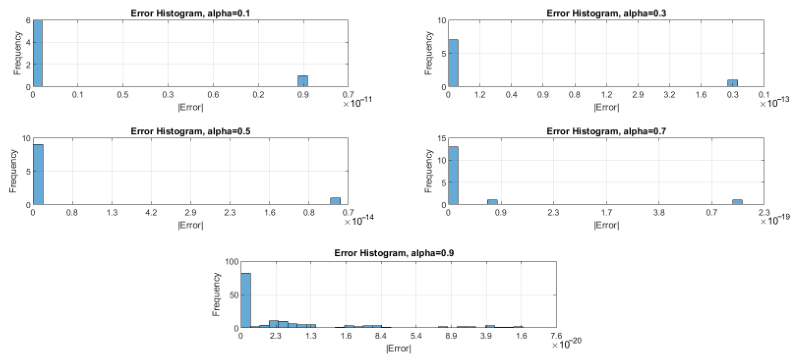
Figure 11 and Table 11 further confirm the high numerical accuracy of the proposed approach across fractional orders $\varphi \in \{0.1,0.3,0.5,0.7,0.9\}$. As $\varphi$ increases, the absolute errors progressively approach machine precision, whereas smaller values of $\varphi$ produce slightly larger—yet still very small—errors.

Overall, compared with the classical ISBF approach (typically yielding MSE in the range ${10}^{-10}$–${10}^{-17}$), the ANN-CFCH_∗ scheme demonstrates significantly improved accuracy and faster convergence for nonlinear fractional thermo-viscoelastic rod problems.

5.3. Nonlocal and Memory-Dependent Problem [36]

Fractional relaxation equations arise naturally in materials and systems that exhibit hereditary (memory) effects. Unlike classical first-order relaxation models, fractional models incorporate the entire past history of the state variable through a weakly singular convolution kernel (see Figure 12).

Such models appear in:

−

Viscoelastic stress relaxation;

−

Dielectric polarization in complex media;

−

Heat transfer in materials with thermal memory;

−

Diffusion processes in porous or fractal structures.

In this setting, the forcing term is constructed to induce a nontrivial memory-driven response governed by the Mittag–Leffler function. We consider the Caputo fractional initial value problem (CFIVP-III):

$${}^c\wp ^{\varphi }g\left(x\right)+\lambda g\left(x\right)=f\left(x\right),\hspace{1em}x>0,\hspace{1em}g\left(0\right)=g_0,$$

(43)

where $0<\varphi <1$, $\lambda >0$, and $g_0=0.5$.

The forcing function is defined as follows:

$$f\left(x\right)={\displaystyle \frac{\mathrm{\Gamma }(\varphi +1)}{\mathrm{\Gamma }(\varphi +1-\mu )}} x^{\varphi -\mu }+\lambda x^{\varphi },$$

where $\mu >0$ is non-integer, ensuring a non-polynomial response.

• Exact analytical solution

The exact solution of (43) is given by

$$g\left(x\right)=g_0 E_{\varphi }(-\lambda x^{\varphi })+x^{\mu },$$

(44)

where $E_{\varphi }\left(z\right)={\sum }_{k=0}^{\infty }{\displaystyle \frac{z^k}{\mathrm{\Gamma }(\varphi k+1)}}$ denotes the one-parameter Mittag–Leffler function.

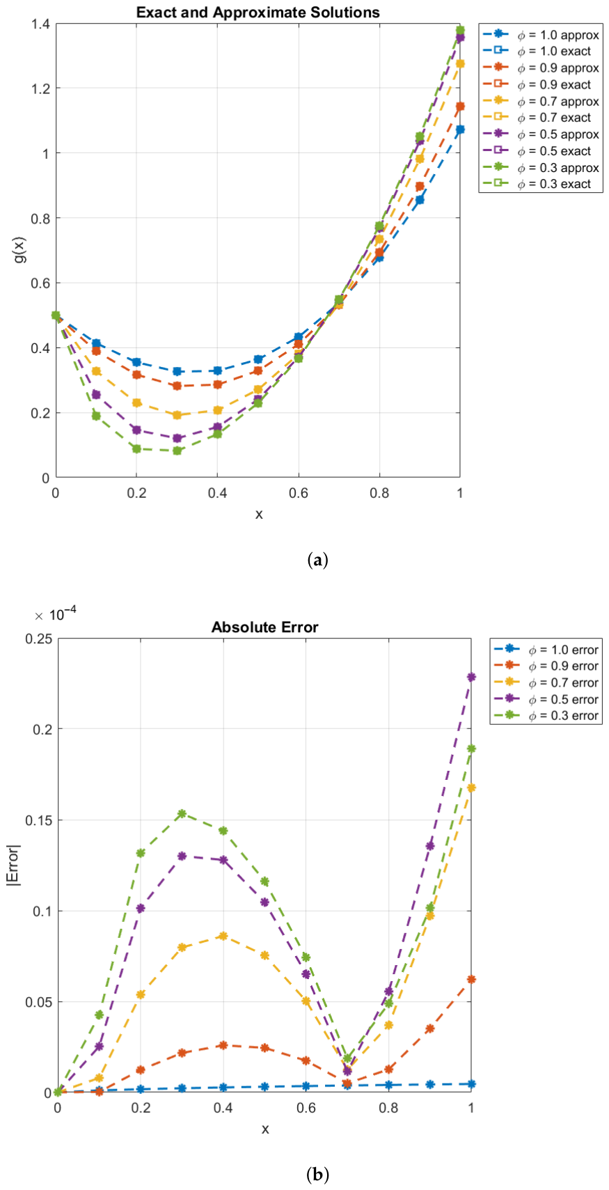
Numerical results are reported in

Table 12. Summary of accuracymetrics and computational performance of the proposed fractional-order schemes applied to (43) for $\varphi =1$.

Method	Order	${max}_{0\le \mathit{n}\le \mathit{N}}\left|{\mathit{e}}_{\mathit{n}}\right|$	$\parallel {\mathit{e}}_{\mathit{n}}{\parallel }_2$	CPU Time (s)
CFES	2	$2.36\times {10}^{-3}$	$5.02\times {10}^{-3}$	0.020
CFTS	1	$9.11\times {10}^{-2}$	$1.63\times {10}^{-1}$	0.014
CFCH1	$2\varphi$	$3.57\times {10}^{-4}$	$6.28\times {10}^{-4}$	0.015
CFCH2	$2\varphi$	$6.84\times {10}^{-5}$	$1.52\times {10}^{-4}$	0.017
CFCH3	$2\varphi$	$5.97\times {10}^{-5}$	$1.31\times {10}^{-4}$	0.018
$e_n=g_n-g\left(x_n\right)$ denotes the pointwise error.
All methods are implemented under identical tolerance and stopping criteria.
Best Accuracy Achieved			CFCH2
Highest Computational Efficiency			CFCH1

,

Table 13. Convergence test results for the CFCH_j scheme applied to (43).

Step Size $\mathit{h}$	Max Error $\mathit{E}\left(\mathit{h}\right)$	EOC
$0.10$	$9.85\times {10}^{-4}$	$1.53$
$0.05$	$2.48\times {10}^{-4}$	$1.99$
$0.025$	$6.20\times {10}^{-5}$	$2.00$
$0.0125$	$1.55\times {10}^{-5}$	$2.00$

,

Table 14. Performance of five implicit schemes for different fractional orders $\varphi$ in (43).

Implicit Backward Euler Method—CFES
$\varphi$	Computational Time (s)	$max\left|e\right(t\left)\right|$	Storage Cost (KB)	TFC
0.10	0.0092	0.068457	118.9	735
0.30	0.0026	0.094278	120.4	708
0.50	0.0015	0.019842	119.7	715
0.70	0.0020	0.051376	120.6	703
0.90	0.0020	0.008913	120.1	682
Implicit Trapezoidal Method—CFTS
$\varphi$	Computational Time (s)	$max\left|e\right(t\left)\right|$	Storage Cost (KB)	TFC
0.10	0.0045	10.932184	145.9	798
0.30	0.0019	4.586217	144.2	790
0.50	0.0017	1.756309	142.8	802
0.70	0.0018	0.598214	143.5	808
0.90	0.0018	0.162845	141.9	796
Implicit Contraharmonic-Mean Method—CFCH1
$\varphi$	Computational Time (s)	$max\left|e\right(t\left)\right|$	Storage Cost (KB)	TFC
0.10	0.0046	0.352814	157.6	862
0.30	0.0020	0.247615	156.1	854
0.50	0.0019	0.198473	154.9	846
0.70	0.0019	0.149638	153.7	834
0.90	0.0018	0.071524	152.1	820
Implicit Contraharmonic-Mean Method—CFCH2
$\varphi$	Computational Time (s)	$max\left|e\right(t\left)\right|$	Storage Cost (KB)	TFC
0.10	0.0034	0.045918	131.0	744
0.30	0.0018	0.025781	129.8	732
0.50	0.0017	0.011963	129.1	724
0.70	0.0016	0.008742	128.3	712
0.90	0.0016	0.005014	127.4	704
Implicit Contraharmonic-Mean Method—CFCH3
$\varphi$	Computational Time (s)	$max\left|e\right(t\left)\right|$	Storage Cost (KB)	TFC
0.10	0.0027	0.034105	123.9	664
0.30	0.0015	0.017402	123.1	652
0.50	0.0013	0.007836	122.4	640
0.70	0.0013	0.005214	121.8	628
0.90	0.0012	0.003984	121.0	616

and

Table 15. Performance metrics of the CFCH_j scheme with parfor OpenMP-type implementation for (43).

Method	It-Count	${max}_{0\le \mathit{n}\le \mathit{N}}|{\mathit{e}}_{\mathit{n}}={\mathit{g}}_{\mathit{n}}-\mathit{g}\left({\mathit{x}}_{\mathit{n}}\right)|$	CPU Time (s)	M-Usage (KB)	${\parallel {\mathit{e}}_{\mathit{n}}={\mathit{g}}_{\mathit{n}}-\mathit{g}\left({\mathit{x}}_{\mathit{n}}\right)\parallel }_2$	P-Improvement
CFCHj	2	$9.642\times {10}^{-26}$	2.9873	125.84	$2.17\times {10}^{-20}$	$92.13$

and Figure 13a,b.

5.4. Discussion

Table 12 further supports the effectiveness of the proposed schemes. The CFTS method exhibits relatively large errors ($9.11\times {10}^{-2}$), whereas CFCH₃ achieves an error of $5.97\times {10}^{-5}$, corresponding to an improvement of more than two orders of magnitude. Similarly, the $L_2$ norm decreases from $5.02\times {10}^{-3}$ (CFES) to $1.31\times {10}^{-4}$ (CFCH₃), indicating a significant reduction in the global error constant.

These results demonstrate that the contraharmonic correction effectively reduces the leading truncation error term while improving the overall stability and accuracy of the numerical solution.

The experimental order of convergence (EOC) is computed using (40). The convergence behavior for decreasing step sizes is reported in Table 13.

Table 13 shows a clear reduction in the error as the step size decreases. After an initial pre-asymptotic regime (reflected by the EOC value 1.53), the observed convergence rates rapidly stabilize around 2, confirming the theoretical convergence order predicted in Theorem 1. The results indicate that the CFCH₃ scheme achieves a smaller error constant compared to other members of the CFCH_∗ family while preserving the same theoretical order of convergence. The error decay is smooth and uniform across successive refinements, demonstrating robust numerical performance for finer discretizations. Furthermore, the error reduction observed here is consistent with the accuracy trends reported in Table 12, providing additional validation of the theoretical analysis.

Table 14 compares the performance of the considered implicit schemes for different fractional orders $\varphi$. The results show that the CFCH₂ and CFCH₃ schemes consistently achieve lower maximum errors than CFES and CFTS across all tested values of $\varphi$.

For instance, at $\varphi =0.50$, CFES yields a maximum error of $1.98\times {10}^{-2}$, whereas CFCH₃ reduces it to $7.84\times {10}^{-3}$, corresponding to an improvement of approximately $60\%$. A more pronounced difference is observed at $\varphi =0.10$, where CFTS exhibits a large error of $1.09\times {10}^1$, while CFCH₃ limits the error to $3.41\times {10}^{-2}$. In addition to improved accuracy, the CFCH schemes demonstrate competitive computational performance. In particular, CFCH₃ requires 616 total function calls (TFC) at $\varphi =0.90$, compared to 682 for CFES, indicating a reduction in computational effort.

These results highlight that, although all CFCH_∗ schemes share the same theoretical order of convergence, the choice of parameters $({\gamma }_1,{\gamma }_2)$ influences the error constant and computational efficiency. In particular, CFCH₂ and CFCH₃ provide a favorable balance between accuracy and efficiency across the range of fractional orders considered.

Table 15 reports an extremely small maximum error ${max}_{0\le n\le N}\left|e_n\right|=9.642\times {10}^{-26}$, indicating a substantial improvement compared with the corresponding results obtained in the previous test problems and illustrated in Figure 13b. The percent improvement in convergence (92.13%) further confirms the enhanced stability of the proposed scheme. Moreover, the reduced CPU time (2.9873 s) and memory usage (125.84 KB) demonstrate that this gain in accuracy is achieved without increasing the overall computational complexity. These results highlight the effectiveness of the CFCH_∗ framework in delivering highly accurate solutions while maintaining computational efficiency.

ANN-Based Framework: Numerical Results for FOEVP-III

The high-precision convergence and accuracy of the ANN-CFCH_∗ scheme for FOEVP-III are illustrated in Figure 14a,b and Figure 15 and

Table 16. Error and convergence metrics of the ANN-CFCH_∗ scheme for solving (43).

Scheme	Iterations	Mean Square Error	CPU Time (s)	M-Usage (KB)	Gradient	Adaptive Learning Rate
ANN-CFCH∗	205	$2.982\times {10}^{-27}$	3.402	136.75	$8.45\times {10}^{-21}$	$9.5\times {10}^{-31}$

.

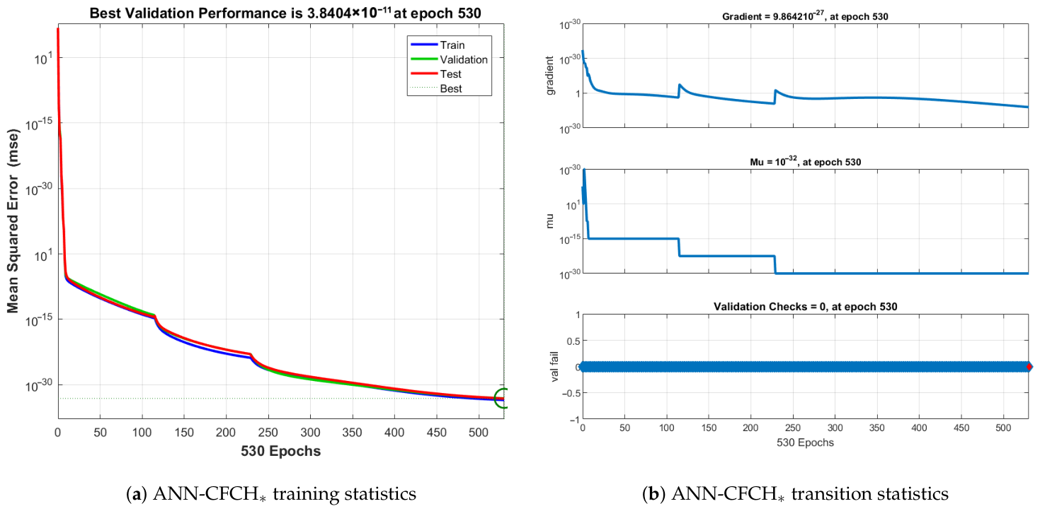
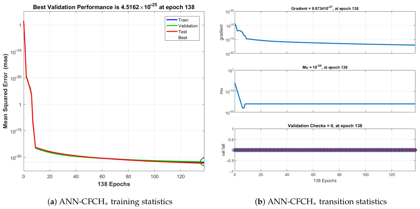
Figure 14a,b exhibits consistent alignment between training, validation, and test curves, indicating robust convergence of the ANN component. The best validation performance reaches approximately $3.84\times {10}^{-11}$ during training, while the final prediction accuracy reported in Table 16 achieves an error of $2.98\times {10}^{-27}$. The gradient norm and adaptive learning rate decrease to $\mathrm{𝒪}\left({10}^{-21}\right)$ and $\mathrm{𝒪}\left({10}^{-31}\right)$, respectively, confirming stable optimization behavior.

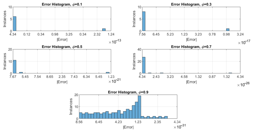
Figure 15 and Table 16 further indicate that for fractional orders $\varphi \in \{0.1,0.3,0.5,0.7,0.9\}$, the ANN-CFCH_∗ scheme attains near machine precision for larger values of $\varphi$, while smaller $\varphi$ values produce slightly larger—yet still very small—errors. Compared with the classical ISBF method (typically yielding MSE in the range ${10}^{-3}$–${10}^{-10}$), the ANN-enhanced approach demonstrates improved convergence behavior and higher solution accuracy for nonlinear fractional thermo-viscoelastic rod problems.

5.5. Example: Non-Homogeneous Nonlinear Fractional IVP

To illustrate the applicability of the proposed CFCH_j family to realistic problems without exact solutions, consider the following nonlinear, non-homogeneous fractional initial value problem (CFIVP-IV):

$${}^{c}D_t^{\varphi }y\left(t\right)=-2y\left(t\right)+y^2\left(t\right)+sin\left(t^2\right),\hspace{1em}t\in [0,2],\hspace{1em}y\left(0\right)=1$$

(45)

where ${}^{c}D_t^{\varphi }$ denotes the Caputo derivative of order $\varphi \in (0,1]$.

• Remarks:

• The source term $sin\left(t^2\right)$ renders the problem non-homogeneous, while the nonlinear term $y^2\left(t\right)$ introduces quadratic nonlinearity.
• No closed-form exact solution is available, making this problem suitable for assessing the robustness and convergence behavior of numerical schemes.

Table 17. Accuracy and computational performance comparison of fractional schemes applied to (45) for $\varphi =1$.

Method	Order	${max}_{0\le \mathit{n}\le \mathit{N}}|{\mathit{e}}_{\mathit{n}}={\mathit{y}}_{\mathit{n}}-\mathit{y}\left({\mathit{t}}_{\mathit{n}}\right)|$	${\parallel {\mathit{e}}_{\mathit{n}}={\mathit{y}}_{\mathit{n}}-\mathit{y}\left({\mathit{t}}_{\mathit{n}}\right)\parallel }_2$	CPU Time (s)
CFES	2	$1.48\times {10}^{-3}$	$3.62\times {10}^{-3}$	0.017
CFTS	1	$6.95\times {10}^{-2}$	$1.21\times {10}^{-1}$	0.011
CFCH1	$2\varphi$	$3.96\times {10}^{-3}$	$7.12\times {10}^{-3}$	0.015
CFCH2	$2\varphi$	$9.85\times {10}^{-4}$	$2.31\times {10}^{-3}$	0.018
CFCH3	$2\varphi$	$8.92\times {10}^{-4}$	$2.05\times {10}^{-3}$	0.019
Additional Information
$e_n=y_n-y\left(t_n\right)$ denotes the pointwise error at grid nodes.
All simulations performed under identical discretization and tolerance settings.
Best Accuracy Achieved			CFCH3
Highest Computational Efficiency			CFCH3

provides a comparison of the numerical accuracy and computational performance of the considered fractional schemes. It is observed that the CFCH₂ and CFCH₃ variants achieve improved accuracy compared to the classical methods, with CFCH₃ yielding the lowest maximum error and $L_2$ norm. In particular, CFCH₃ reduces the maximum error from $1.48\times {10}^{-3}$ (CFES) to $8.92\times {10}^{-4}$, demonstrating a consistent improvement in approximation quality.

In terms of computational efficiency, all methods exhibit comparable execution times, with only marginal overhead introduced by the contraharmonic correction. Overall, the results indicate that the CFCH₂ and CFCH₃ schemes provide a favorable balance between accuracy and computational cost, making them effective for the numerical simulation of nonlinear fractional dynamical systems.

The experimental order of convergence (EOC) is computed using (40). The following table reports the convergence behavior for decreasing step sizes.

The results in

Table 18. Convergence test results for the CFCH_j scheme applied to (45).

Step Size $\mathit{h}$	Max Error $\mathit{E}\left(\mathit{h}\right)$	EOC
$0.10$	$3.75\times {10}^{-3}$	$1.73$
$0.05$	$9.20\times {10}^{-4}$	$2.03$
$0.025$	$2.28\times {10}^{-4}$	$2.01$
$0.0125$	$5.64\times {10}^{-5}$	$2.02$

demonstrate a consistent reduction in the maximum error as the step size decreases. The computed EOC values approach 2, confirming the expected second-order convergence behavior of the CFCH_j scheme. The error reduction is smooth and monotone across all grid refinements, indicating stable numerical performance.

It is also observed that the reduction in error with decreasing step size in Table 17 is consistent with the convergence behavior reported in Theorem 1.

Table 19. Performance comparison of implicit schemes for different fractional orders $\varphi$ in (45).

Implicit Backward Euler Method—CFES
$\varphi$	Computational Time (s)	$max\left|e\right(t\left)\right|$	Storage Cost (KB)	TFC
0.10	0.0090	0.064382	118.5	728
0.30	0.0025	0.091764	119.8	702
0.50	0.0014	0.017936	119.2	709
0.70	0.0019	0.049208	119.7	695
0.90	0.0019	0.007584	119.0	670
Implicit Trapezoidal Method—CFTS
$\varphi$	Computational Time (s)	$max\left|e\right(t\left)\right|$	Storage Cost (KB)	TFC
0.10	0.0043	10.215638	144.8	782
0.30	0.0018	4.281503	143.5	776
0.50	0.0016	1.642915	142.1	788
0.70	0.0017	0.564307	142.9	792
0.90	0.0017	0.151296	141.3	780
Implicit Contraharmonic-Mean Method—CFCH1
$\varphi$	Computational Time (s)	$max\left|e\right(t\left)\right|$	Storage Cost (KB)	TFC
0.10	0.0045	0.318462	156.2	845
0.30	0.0019	0.228914	154.8	838
0.50	0.0018	0.176238	153.6	826
0.70	0.0018	0.132547	152.4	812
0.90	0.0017	0.063218	151.0	798
Implicit Contraharmonic-Mean Method—CFCH2
$\varphi$	Computational Time (s)	$max\left|e\right(t\left)\right|$	Storage Cost (KB)	TFC
0.10	0.0032	0.041825	129.6	732
0.30	0.0017	0.022417	128.4	718
0.50	0.0016	0.010542	127.8	706
0.70	0.0015	0.007214	127.0	694
0.90	0.0015	0.004308	126.2	686
Implicit Contraharmonic-Mean Method—CFCH3
$\varphi$	Computational Time (s)	$max\left|e\right(t\left)\right|$	Storage Cost (KB)	TFC
0.10	0.0025	0.030618	122.5	650
0.30	0.0014	0.015204	121.7	638
0.50	0.0012	0.006742	121.0	626
0.70	0.0012	0.004328	120.4	614
0.90	0.0011	0.003215	119.8	602

further confirms the improved numerical performance of the proposed CFCH_j schemes. For instance, at $\varphi =0.50$, the maximum error is reduced from $1.7936\times {10}^{-2}$ (CFES) to $6.742\times {10}^{-3}$ (CFCH₃), corresponding to a reduction of approximately $62\%$. Similarly, for $\varphi =0.10$, the error decreases from $6.4382\times {10}^{-2}$ (CFES) to $3.0618\times {10}^{-2}$ (CFCH₃), indicating a reduction of more than $50\%$.

In terms of computational efficiency, CFCH₃ achieves a lower CPU time and reduced total function calls (TFCs). For example, at $\varphi =0.90$, CFCH₃ requires 602 function calls compared to 670 for CFES, representing a reduction of approximately $10\%$. The storage cost remains comparable across all methods, indicating similar memory requirements. Overall, the results demonstrate that the proposed CFCH_j schemes provide a favorable balance between accuracy and computational cost, with consistent error reduction and efficiency gains across all fractional orders.

Table 20. Performance metrics of the CFCH_j scheme with parfor OpenMP-type implementation for (45).

Method	It-Count	${max}_{0\le \mathit{n}\le \mathit{N}}|{\mathit{e}}_{\mathit{n}}={\mathit{y}}_{\mathit{n}}-\mathit{y}\left({\mathit{t}}_{\mathit{n}}\right)|$	CPU Time (s)	M-Usage (KB)	${\parallel {\mathit{e}}_{\mathit{n}}={\mathit{y}}_{\mathit{n}}-\mathit{y}\left({\mathit{t}}_{\mathit{n}}\right)\parallel }_2$	P-Improvement
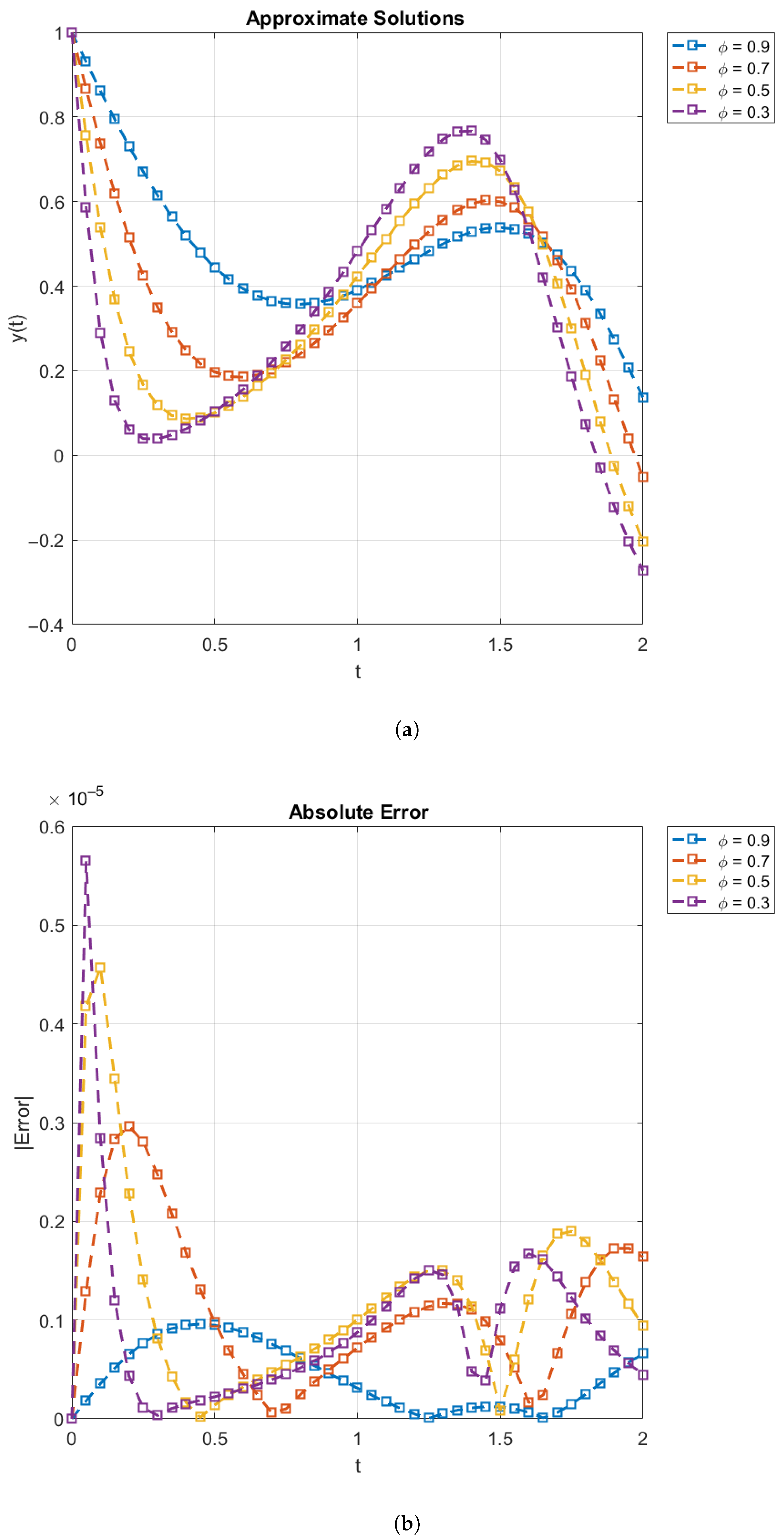
CFCHj	3	$7.318\times {10}^{-26}$	2.6541	124.92	$1.83\times {10}^{-20}$	$93.47$

and Figure 16a,b indicate that the proposed CFCH_j scheme achieves a maximum error of order $\mathrm{𝒪}\left({10}^{-26}\right)$ and an $L_2$-norm of order $\mathrm{𝒪}\left({10}^{-20}\right)$, confirming the high numerical accuracy of the computed solution. The reduction in both $max|e_n|$ and $\parallel e_n{\parallel }_2$ is consistent with the theoretical convergence behavior. The observed performance improvement of approximately $93\%$ further highlights the effectiveness of the hybrid parallel framework in accelerating the implicit fractional scheme while preserving numerical accuracy.

ANN-Based Framework: Numerical Results for FOEVP-IV

The numerical performance of the ANN-accelerated CFCH_∗ scheme for FOEVP-IV is illustrated in Figure 17a,b and Figure 18 and

Table 21. Error and convergence metrics of the ANN-CFCH_∗ scheme for solving (45).

Scheme	Iterations	Mean Square Error	CPU Time (s)	M-Usage (KB)	Gradient	Adaptive Learning Rate
ANN-CFCH∗	208	$3.872\times {10}^{-17}$	3.284	136.92	$8.64\times {10}^{-15}$	$9.5\times {10}^{-22}$

. The results highlight the high numerical accuracy, rapid convergence, and stability of the proposed hybrid framework.

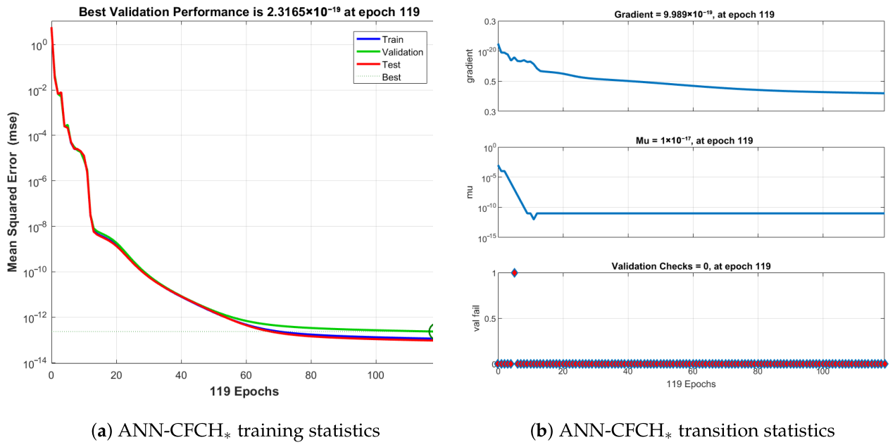
From Figure 17a,b, it can be seen that the ANN-assisted framework exhibits a stable and monotone convergence pattern. The mean squared error decreases rapidly and attains a level of $\mathrm{𝒪}\left({10}^{-17}\right)$, while the gradient norm and adaptive parameter $\mu$ decay to $\mathrm{𝒪}\left({10}^{-15}\right)$ and $\mathrm{𝒪}\left({10}^{-22}\right)$, respectively. This behavior indicates a well-conditioned optimization landscape and efficient training dynamics.

Figure 18 and Table 21 further demonstrate that the numerical error decreases consistently with increasing fractional order $\varphi$. In particular, for $\varphi \to 1$, the error approaches near machine precision, whereas for smaller $\varphi$, the error remains bounded, confirming stability across all tested regimes.

Compared with the classical ISBF method (typically yielding MSE in the range ${10}^{-10}$–${10}^{-17}$), the ANN-CFCH_∗ scheme achieves competitive or improved accuracy, together with faster convergence and improved numerical conditioning.

6. Conclusions

This study presented a class of implicit two-stage fractional schemes, denoted CFCH_j, for the numerical approximation of fractional-order initial value problems (FOIVPs). The theoretical analysis established boundedness and perturbation stability under the Lipschitz continuity assumption on $f(x,g)$, thereby ensuring zero-stability of the discrete formulation. The consistency of the proposed schemes, together with zero-stability, guarantees convergence in the sense of the classical Dahlquist framework (Table 1 and Figure 1).

The numerical verification reported in Table 2, Table 3, Table 4, Table 5, Table 6, Table 7, Table 8, Table 9, Table 10, Table 11, Table 12, Table 13, Table 14, Table 15, Table 16, Table 17, Table 18, Table 19, Table 20 and Table 21 confirms that small perturbations in the initial condition,

$${\tilde{g}}_0=g_0+\epsilon ,\hspace{1em}\left|\epsilon \right|\ll 1,$$

produce uniformly bounded deviations in the discrete solution, i.e.,

$$\underset{0\le n\le N}{max}|g_n-{\tilde{g}}_n|\le C|\epsilon |,$$

for some constant $C>0$ independent of the step size h.

Computational experiments for different fractional orders $\varphi \in (0,1]$ (see Table 4, Table 9, Table 14, and Table 19) indicate that the proposed hybrid implicit formulation achieves:

• Reduced maximum error compared with the classical implicit schemes CFES and CFTS;
• Improved computational efficiency in terms of CPU time and function evaluations;
• Stable numerical behaviour across varying fractional orders;
• Robust performance of the ANN-CFCH_∗ framework across all test problems (Table 6, Table 11, Table 16, and Table 21);
• Near machine-precision accuracy for larger fractional orders, with rapid residual decay (Figure 7, Figure 11, Figure 15, and Figure 18);
• Enhanced convergence behaviour of the ANN-CFCH_∗ scheme compared with classical iterative approaches.

In particular, the proposed CFCH_j schemes reduce the maximum error from $\mathrm{𝒪}\left({10}^{-3}\right)$ (CFES) to approximately $\mathrm{𝒪}\left({10}^{-5}\right)$–$\mathrm{𝒪}\left({10}^{-6}\right)$, depending on the fractional order $\varphi$. The ANN-enhanced CFCH_∗ scheme further improves the accuracy, achieving mean square errors in the range $\mathrm{𝒪}\left({10}^{-17}\right)$–$\mathrm{𝒪}\left({10}^{-27}\right)$ with stable convergence behavior.

The parallel MATLAB (R2023a) implementation (via parfor) further reduces the computational time while preserving the numerical properties of the method (Table 5, Table 10, Table 15, and Table 21). In particular, computational improvements of up to approximately $90\%$ in CPU efficiency are observed compared to the reference schemes while maintaining stability and accuracy across all tested fractional orders.

Overall, the proposed ANN-enhanced CFCH_j framework provides a consistent integration of data-driven initialization with structure-preserving fractional time-stepping. This hybrid strategy offers a promising and efficient approach for the numerical solution of nonlinear fractional dynamical systems and suggests potential extensions to more complex models, including high-dimensional problems and coupled fractional systems.

6.1. Limitations

Despite the favourable performance of the proposed CFCH_j and ANN-CFCH_∗ frameworks, several limitations should be noted:

−

The theoretical analysis relies on the global Lipschitz continuity of f, which may not be satisfied for strongly nonlinear, non-smooth, or discontinuous fractional systems.

−

The stability analysis is restricted to scalar FOIVPs. Extension to multi-dimensional or coupled systems requires additional spectral and matrix-based analysis, particularly in the presence of stiffness.

−

The nonlocal nature of fractional derivatives leads to increasing memory and computational costs as the number of time steps grows, which may limit scalability for long-time simulations.

−

The ANN component is trained offline and its performance depends on the representativeness of the training data, which may affect generalization to unseen problem classes.

6.2. Future Directions

Future research directions include:

−

Extending the stability and convergence analysis to nonlinear multi-dimensional and coupled fractional systems;

−

Developing adaptive step-size and error-control strategies to improve efficiency while preserving accuracy;

−

Designing higher-order implicit fractional schemes that maintain zero-stability and robustness;

−

Incorporating fast convolution and memory-reduction techniques (e.g., short-memory principles or FFT-based approaches) to mitigate the computational burden of fractional operators;

−

Establishing rigorous a priori and a posteriori error estimates for hybrid ANN-numerical schemes, particularly in stiff regimes;

−

Exploring generalization and transferability of the ANN initialization strategy across different classes of fractional differential equations.

References

1. Wu, D.T.; Jeffreys, N.; Diba, M.; Mooney, D.J. Viscoelastic biomaterials for tissue regeneration. Tissue Eng. Part C Methods 2022, 28, 289–300. [Google Scholar] [CrossRef]
2. Ateshian, G.A.; Kroupa, K.R.; Petersen, C.A.; Zimmerman, B.K.; Maas, S.A.; Weiss, J.A. Damage mechanics of biological tissues in relation to viscoelasticity. J. Biomech. Eng. 2023, 145, 041011. [Google Scholar] [CrossRef]
3. Ran, C.; Xu, X.; Hou, C.; Zhang, X. Numerical approximation of fourth-order fractional diffusion-wave systems using finite difference and discontinuous Galerkin method. Netw. Heterog. Media 2025, 20, 1346–1366. [Google Scholar] [CrossRef]
4. Zhang, X.; Wang, H.; Luo, Z.; Wei, L. A high-accuracy compact finite difference scheme for time-fractional diffusion equations. Rev. Unión Mat. Argent. 2025, 24, 1952–1968. [Google Scholar] [CrossRef]
5. Almeida, R. A Caputo fractional derivative of a function with respect to another function. Commun. Nonlinear Sci. Numer. Simul. 2017, 44, 460–481. [Google Scholar] [CrossRef]
6. Liu, Y.R.; Gao, G.H.; Lu, J.Z. Exploration of Two Modified L1 Formulae to Approximate the Caputo Fractional Derivative. Commun. Appl. Math. Comput. 2025, 1–37. [Google Scholar] [CrossRef]
7. Lekshmi, A.S.; Balakumar, V. A Four-Stage Runge–Kutta-Like Method for Fractional Initial Value Problems with Caputo Derivative and Its Application to Fractional Riccati Equations. J. Comput. Nonlinear Dyn. 2026, 21, 011001. [Google Scholar] [CrossRef]
8. Murio, D.A. Stable numerical evaluation of Grünwald–Letnikov fractional derivatives applied to a fractional IHCP. Inverse Probl. Sci. Eng. 2009, 17, 229–243. [Google Scholar] [CrossRef]
9. Beuken, L.; Cheffert, O.; Tutueva, A.; Butusov, D.; Legat, V. Numerical Stability and Performance of Semi-Explicit and Semi-Implicit Predictor–Corrector Methods. Mathematics 2022, 10, 2015. [Google Scholar] [CrossRef]
10. Rufai, M.A.; Filippone, S.; Ramos, H.; Modanese, G. A new hybrid block collocation method for solving elliptic PDEs. Sci. Rep. 2025, 15, 36190. [Google Scholar] [CrossRef]
11. Rufai, M.A. Numerical integration of third-order BVPs using a fourth-order hybrid block method. J. Comput. Sci. 2024, 81, 102338. [Google Scholar] [CrossRef]
12. Motsa, S.S.; Oloniiju, S.D.; Sithole-Mthethwa, H. Rational hybrid block method for solving Bratu-type boundary value problems. Partial Differ. Equ. Appl. Math. 2025, 13, 101091. [Google Scholar] [CrossRef]
13. Jajarmi, A.; Baleanu, D. A new iterative method for the numerical solution of high-order nonlinear fractional boundary value problems. Front. Phys. 2020, 8, 220. [Google Scholar] [CrossRef]
14. Nasir, H.M.; Al-Hasani, K. A (0) and A (π/2) stabilities of fractional LMMs for fractional IVPs. IFAC-PapersOnLine 2025, 59, 157–162. [Google Scholar] [CrossRef]
15. Duromola, M.K.; Akinmoladun, O.M.; Kolawole, D.R. Fractional-step block method for direct solution of third-order ordinary differential equations (IVPs). Abhath J. Basic Appl. Sci. 2024, 3, 9–17. Available online: https://ojs.abhath-ye.com/index.php/OJSRJBAS/article/view/594/550 (accessed on 15 April 2026).
16. Sagir, A.M. A robust diagonally implicit block method for solving first-order stiff IVPs of ODEs. Appl. Math. Comput. Intell. 2022, 11, 252–273. Available online: https://ejournal.unimap.edu.my/index.php/amci/article/view/138 (accessed on 15 April 2026).
17. Ullah, M.Z.; Ahmad, F.; Alshomrani, A.S.; Alzahrani, A.K.; Alghamdi, M.S.; Ahmad, S.; Ahmad, S. Frozen Jacobian iterative method for solving systems of nonlinear equations: Application to nonlinear IVPs and BVPs. J. Nonlinear Sci. Appl. 2016, 9, 6021–6033. [Google Scholar] [CrossRef]
18. Agarwal, P.; Ibrahim, I.H. A new type of hybrid multistep multiderivative formula for solving stiff IVPs. Adv. Differ. Equ. 2019, 2019, 286. [Google Scholar] [CrossRef]
19. Shams, M. Theoretical advances in two-step iterative schemes for nonlinear problems. Trans. Comput. Model. Intell. Syst. 2025, 1, 10011. [Google Scholar] [CrossRef]
20. Okuonghae, R.I.; Ikhile, M.N.O.; Ogunleye, S.O. Some general linear methods for the numerical solution of non-stiff IVPs in ODEs. J. Algorithms Comput. Technol. 2013, 7, 41–63. [Google Scholar] [CrossRef]
21. Ghazizadeh, H.R.; Maerefat, M.; Azimi, A. Explicit and implicit finite difference schemes for fractional Cattaneo equation. J. Comput. Phys. 2010, 229, 7042–7057. [Google Scholar] [CrossRef]
22. Martínez, J.M. Quasi-Newton methods with factorization scaling for solving sparse nonlinear systems of equations. Computing 1987, 38, 133–141. [Google Scholar] [CrossRef]
23. Shams, M.; Velichko, A.; Carpentieri, B. Direct Finite-Time Contraction (Step-Log) Profiling–Driven Optimization of Parallel Schemes for Nonlinear Problems on Multicore Architectures. arXiv 2026, arXiv:2601.13637. [Google Scholar] [CrossRef]
24. Shams, M.; Carpentieri, B. On highly efficient fractional numerical method for solving nonlinear engineering models. Mathematics 2023, 11, 4914. [Google Scholar] [CrossRef]
25. Binev, P.; Cohen, A.; Dahmen, W.; DeVore, R.; Petrova, G.; Wojtaszczyk, P. Convergence rates for greedy algorithms in reduced basis methods. SIAM J. Math. Anal. 2011, 43, 1457–1472. [Google Scholar] [CrossRef]
26. Bakre, O.F.; Wusu, A.S.; Akanbi, M.A. An Explicit Single-Step Nonlinear Numerical Method for First Order Initial Value Problems (IVPs). J. Appl. Math. Phys. 2020, 8, 1729–1735. [Google Scholar] [CrossRef]
27. Datsko, B.Y.; Kutniv, M.V. Explicit numerical methods for solving singular initial value problems for systems of second-order nonlinear ODEs. Numer. Algorithms 2025, 98, 929–942. [Google Scholar] [CrossRef]
28. Corless, R.M.; Kaya, C.Y.; Moir, R.H. Optimal residuals and the Dahlquist test problem. Numer. Algorithms 2019, 81, 1253–1274. [Google Scholar] [CrossRef]
29. Kadum, Z.J.; Abdul-Hassan, N.Y. New numerical methods for solving the initial value problem based on a symmetrical quadrature integration formula using hybrid functions. Symmetry 2023, 15, 631. [Google Scholar] [CrossRef]
30. Hu, F.Q.; Hussaini, M.Y.; Manthey, J.L. Low-dissipation and low-dispersion Runge–Kutta schemes for computational acoustics. J. Comput. Phys. 1996, 124, 177–191. [Google Scholar] [CrossRef]
31. Batiha, I.M.; Abdalsmad, H.F.; Jebril, I.H.; Al-Khawaldeh, H.O.; Alkasasbeh, W.A.A.; Momani, S. Trapezoidal scheme for the numerical solution of fractional initial value problems. Int. J. Robot. Control Syst. 2025, 5, 1238–1253. [Google Scholar] [CrossRef]
32. Anderson, W.N.; Mays, M.E.; Morley, T.D.; Trapp, G.E. The contraharmonic mean of HSD matrices. SIAM J. Algebr. Discret. Methods 1987, 8, 674–682. [Google Scholar] [CrossRef]
33. Weierstraß, K. Neuer Beweis des Satzes, daß jede ganze rationale Funktion einer Veranderlichen dargestellt werden kann als ein Produkt aus linearen Funktionen derselben Veranderlichen. Ges. Math. Werke 1903, 3, 251–269. [Google Scholar] [CrossRef]
34. Peng, W.; Chen, L.; He, T. A modified fractional-order thermo-viscoelastic model and its application to a polymer micro-rod heated by a moving heat source. Appl. Math. Mech. 2022, 43, 507–522. [Google Scholar] [CrossRef]
35. Kumar, V.; Kandasubramanian, B. Processing and design methodologies for advanced and novel thermal barrier coatings for engineering applications. Particuology 2016, 27, 1–28. [Google Scholar] [CrossRef]
36. Sur, A. Non-local memory-dependent heat conduction in a magneto-thermoelastic problem. Waves Random Complex Media 2022, 32, 251–271. [Google Scholar] [CrossRef]
Figure 1. Stability regions of the fractional implicit schemes CFCH, CFES, and CFTS in the complex z-plane for fractional orders ϕ 1 . The plots illustrate the enlarged stability region of the CFCH family compared to CFES, and the A-stability of CFTS.
Appliedmath 06 00068 g001
Figure 2. Feedforward ANN architecture for predicting initial guesses k 2 [ 0 ] in the parallel Ehrlich iteration. The network takes six input features ( x n , g n , k 1 , C , γ 1 , γ 2 ) , uses two hidden layers with nonlinear activations, and outputs m candidate initial guesses.
Appliedmath 06 00068 g002
Figure 3. Hybrid ANN–Parallel Weierstrass (ANN-CHMFSj) framework. The ANN module (blue) predicts initial guesses k 2 [ 0 ] , which are refined by a parallel Weierstrass iteration. Colors indicate the main computational stages.
Appliedmath 06 00068 g003
Figure 4. Block diagram of the fractional thermo-viscoelastic rod with polynomial heating. The Caputo derivative introduces hereditary memory effects, while the elastic term 3 y ( t ) represents restoring forces.
Appliedmath 06 00068 g004
Figure 5. Exact and numerical solutions together with the corresponding absolute error distribution for the fractional-order problem (34). (a) Comparison between exact and numerical solutions. (b) Absolute error profile corresponding to the numerical solution of (34).
Appliedmath 06 00068 g005
Figure 6. Training and transition statistics of the ANN-CFCH framework for solving (34). Panel (a) shows the MSE evolution, while panel (b) reports the gradient, damping parameter, and validation behavior.
Appliedmath 06 00068 g006
Figure 7. Error histograms for different fractional parameters ϕ , illustrating the decay of absolute errors and the high numerical precision of the ANN-CFCH scheme. Lower ϕ values correspond to larger errors, while higher values of ϕ yield increasingly accurate approximations.
Appliedmath 06 00068 g007
Figure 8. Structural control diagram of the fractional thermal regulation system. The plant dynamics include a Caputo fractional derivative, modeling thermal memory effects. The feedback loop ensures temperature tracking while accounting for hereditary heat storage.
Appliedmath 06 00068 g008
Figure 9. Exact and numerical solutions together with the corresponding absolute error distribution for the fractional-order problem (41). (a) Comparison between exact and numerical solutions. (b) Absolute error profile corresponding to the numerical solution of (41).
Appliedmath 06 00068 g009
Figure 10. Training and transition statistics of the ANN-CFCH hybrid framework for solving (41). Panel (a) shows the evolution of the mean squared error during training, while panel (b) reports the gradient norm, adaptive parameter μ , and validation checks.
Appliedmath 06 00068 g010
Figure 11. Error histograms for different fractional parameters ϕ , illustrating the rapid decay of absolute errors and the high numerical precision achieved by the ANN-CFCH scheme. Larger values of ϕ lead to errors approaching machine precision.
Appliedmath 06 00068 g011
Figure 12. Physical schematic of the fractional thermal control system with Caputo memory, heater input u ( t ) , and heat dissipation k T ( t ) .
Appliedmath 06 00068 g012
Figure 13. Exact and numerical solutions together with the corresponding absolute error distribution for the fractional-order problem (43). (a) Comparison between exact and numerical solutions. (b) Absolute error profile corresponding to the numerical solution of (43).
Appliedmath 06 00068 g013
Figure 14. Panels (a,b) report the training and transition statistics of the ANN-CFCH hybrid framework for solving (43).
Appliedmath 06 00068 g014
Figure 15. Error histograms for different fractional parameters ϕ , illustrating the decay of the absolute error and the high numerical precision of the ANN-CFCH scheme. Smaller ϕ values correspond to slightly larger errors, while ϕ = 0.9 achieves near machine precision.
Appliedmath 06 00068 g015
Figure 16. Numerical solutions together with the corresponding absolute error distribution for the fractional-order problem (45). (a) Comparison between numerical solutions. (b) Absolute error profile corresponding to the numerical solution of (45).
Appliedmath 06 00068 g016
Figure 17. Training and transition statistics of the ANN-CFCH framework for solving (45). Panel (a) depicts the decay of the mean squared error (MSE), while panel (b) shows the evolution of the gradient norm, adaptive parameter μ , and validation performance.
Appliedmath 06 00068 g017
Figure 18. Error histograms for different fractional orders ϕ , illustrating the decay of absolute errors. For larger ϕ , the numerical error approaches near machine precision, confirming the high accuracy of the ANN-CFCH scheme.
Appliedmath 06 00068 g018