A Modular Spatial–Temporal Approach for Territorial Segmentation and Short-Term Crime Prediction

Abstract

Crime forecasting in heterogeneous urban contexts remains challenging due to the combined effects of territorial heterogeneity and complex temporal dynamics. However, a large portion of the existing literature tends to address territorial segmentation and predictive modeling separately, or to combine them within unified workflows that may obscure their distinct analytical roles. This study presents a modular spatial–temporal analytical approach that treats territorial segmentation and short-term crime prediction as complementary but methodologically independent components. Unsupervised segmentation captures territorial heterogeneity, while a supervised ensemble model estimates short-term crime occurrence. A chronological expanding-window validation scheme is implemented, reserving the most recent period as a blind test set to prevent temporal leakage. Across municipalities, recall values in 2022 range from 0.36 to 0.77, with corresponding F1-scores ranging from 0.174 to 0.696, while blind-test recall ranges from 0.184 to 0.856, with F1-scores ranging from 0.000 to 0.784, and AUC values up to 0.88, indicating that predictive performance is context-dependent rather than uniform. The proposed approach provides a replicable and context-aware analytical approach for spatially differentiated crime risk estimation under strict forward-looking evaluation.

1. Introduction

Crime represents one of the most pressing challenges for public security and social development, particularly in urban contexts characterized by strong territorial heterogeneity and dynamic temporal patterns. In Mexico, criminal activity remains at high levels and exhibits pronounced spatial differences across regions and municipalities, complicating the implementation of uniform prevention strategies. In this context, the increasing availability of administrative crime data has enabled the development of data-driven approaches; however, effectively integrating spatial heterogeneity and temporal dynamics remains a persistent challenge.

Traditionally, crime analysis has relied on descriptive statistical methods and explanatory models focused on socioeconomic variables. While these approaches have contributed to understanding structural factors associated with criminal activity, their capacity to capture complex, dynamic, and non-linear patterns is limited. In contrast, machine learning techniques have demonstrated substantial potential for analyzing large, heterogeneous datasets, uncovering latent regularities, and generating predictive estimates in complex environments.

Recent literature identifies two dominant methodological perspectives in data-driven crime analysis. On the one hand, territorial segmentation approaches, commonly implemented through unsupervised clustering techniques, enable the spatial characterization of areas with similar crime profiles and support territorial diagnostics. On the other hand, supervised machine learning models have been widely applied to predict the occurrence of crime events over short-term temporal horizons, emphasizing operational anticipation. However, these approaches are often developed independently, limiting a comprehensive understanding of crime dynamics.

This study proposes an analytical approach that combines both perspectives in a complementary manner, while maintaining a clear conceptual and methodological separation between descriptive spatial analysis and temporal prediction.

It is important to clarify that the proposed framework is designed as a dual but modular analytical structure. Rather than implying a direct feature-level integration, the two components operate with distinct methodological roles: the clustering stage provides a territorial diagnostic, while the predictive model focuses on short-term temporal forecasting.

Importantly, this separation is motivated by a methodological consideration observed in fully integrated spatio-temporal models. When static structural variables are directly incorporated into predictive models, they may interact with short-term temporal signals and influence model behavior under certain validation settings. This consideration motivates the analytical separation adopted in this study, which aims to facilitate a clearer evaluation of temporal dynamics rather than to establish methodological superiority.

By isolating temporal dynamics within the supervised model, the proposed approach enables a more precise evaluation of short-term predictive behavior while preserving spatial structure as an independent diagnostic component. This distinction allows disentangling persistent structural conditions from temporal variation, which is particularly relevant in heterogeneous urban environments where structural conditions and temporal dynamics may operate at different scales.

This methodological independence provides a complementary perspective to feature-level integration approaches. While integrated models aim to maximize predictive performance by combining spatial and temporal features, they may introduce confounding effects between persistent structural conditions and short-term temporal dynamics. In contrast, the proposed approach improves interpretability by allowing each component to be evaluated under its own assumptions, enabling a clearer assessment of predictive behavior under strict chronological validation.

This design choice aims to isolate temporal dynamics and reduce the influence of persistent structural effects in the predictive component. In this context, clustering results are not used as predictive inputs, but instead serve as an interpretive layer to support the understanding of territorial heterogeneity.

The methodology follows the Knowledge Discovery in Databases (KDD) process and is based on official crime records from eleven municipalities in the state of Tamaulipas, Mexico, covering the period from 2017 to 2024.

In the first stage, the K-Means clustering algorithm is applied to segment neighborhoods within each municipality based on crime incidence and socioeconomic characteristics, with the aim of identifying homogeneous territorial patterns. In the second stage, independently of the clustering process, a supervised predictive model based on AdaBoost is implemented to estimate the probability of at least one crime event occurring within 1-, 7-, and 15-day time windows, using temporal and lag-based features derived from historical records.

This study presents an applied modular analytical approach that combines territorial segmentation and temporal prediction as complementary but methodologically independent components, while maintaining a clear separation between descriptive spatial analysis and supervised forecasting. This design enables the generation of interpretable territorial diagnostics and operational short-term risk estimation under a strictly chronological validation scheme. The results show differentiated territorial segmentation patterns and context-dependent predictive performance across municipalities, supporting the relevance of the proposed approach for public security planning and crime prevention strategies.

2. Related Work

Recent literature on data-driven crime analysis can be broadly grouped into two main research lines: territorial segmentation approaches based on unsupervised learning techniques and supervised predictive models aimed at anticipating crime events.

In the first line, several studies have employed clustering algorithms, particularly K-Means, to spatially characterize criminal activity and classify regions or territorial units according to crime incidence. Works such as those by [1,2,3] demonstrate the usefulness of unsupervised clustering for identifying spatial patterns and grouping areas with similar crime profiles. More recent studies have extended spatial clustering approaches by incorporating adaptive density-based methods to better capture heterogeneous crime distributions in urban environments [4]. Complementarily, Refs. [5,6] apply K-Means to segment urban areas and analyze specific crime types, highlighting the descriptive value of clustering techniques for territorial diagnostics.

Other studies have proposed variations or optimizations of the K-Means algorithm to improve clustering quality. For instance, Ref. [7] introduces an optimized K-Means approach for crime analysis and prediction. In the Latin American context, Ref. [8] presents an exploratory analysis supported by machine learning techniques to characterize cybercrime, illustrating the potential of these methods in regions with high territorial heterogeneity.

A second research line focuses on the use of supervised machine learning models for crime prediction. Recent systematic reviews report a growing interest in algorithms such as decision trees, neural networks, ensemble methods, and boosting techniques to anticipate crime occurrence over different temporal horizons [9,10]. These studies emphasize the ability of supervised models to handle large datasets and capture complex, non-linear relationships. Recent work has also explored deep learning architectures for multi-regional crime prediction, highlighting the importance of capturing spatial and temporal dependencies across interconnected areas [11].

Recent applied studies further demonstrate the use of machine learning models for urban crime prediction under real-world conditions. For instance, Ref. [12] integrates multiple data sources and advanced analytical techniques to enhance crime analysis and predictive performance in urban environments.

In addition to purely predictive approaches, alternative system-oriented and knowledge-based methodologies have been proposed. Ref. [13] introduces a semantic reasoning framework for geolocalized crime risk assessment, combining spatial data with knowledge-based models to support decision-making in smart city contexts.

Within this line, AdaBoost has been identified as a competitive approach for crime-related classification tasks, particularly in contexts characterized by class imbalance. Ref. [14] demonstrates the performance of a Naïve Bayes–AdaBoost ensemble for classifying sexual crimes, while other studies report favorable results using machine learning techniques for crime prediction and forecasting [15,16,17].

Despite these advances, most existing studies tend to develop territorial segmentation or predictive modeling approaches either in isolation or within loosely integrated frameworks where the analytical roles of each component are not clearly defined. Clustering-based works primarily focus on spatial characterization and descriptive analysis, without explicitly addressing short-term crime anticipation. Conversely, predictive studies often operate on aggregated spatial units, without incorporating an explicit territorial diagnostic to contextualize their results.

In addition to these two main research lines, recent studies have attempted to integrate multiple analytical components within unified frameworks, combining machine learning, deep learning, and statistical methods for comprehensive crime analysis. For example, Ref. [18] proposes a multi-stage pipeline that includes crime-type classification, temporal forecasting, and regional analysis, while integrated system-oriented approaches emphasize the role of data-driven strategies for proactive crime prevention [19]. While such approaches highlight the potential of combining heterogeneous techniques, they often rely on conventional validation strategies and predefined administrative units, which may limit their ability to capture spatial dependence and ensure robust generalization in real-world predictive settings.

However, explicit modular separation between spatial diagnostic components and temporal predictive modeling remains relatively underexplored in the literature, particularly under strict chronological validation frameworks.

3. Study Area and Data

The study area corresponds to the state of Tamaulipas, located in northeastern Mexico, a region characterized by pronounced territorial heterogeneity in terms of urbanization, economic dynamics, and crime patterns. For analytical purposes, this study focuses on eleven municipalities within the state, which concentrate the complete and consistent availability of crime records throughout the period of analysis. These municipalities include border areas, metropolitan regions, and semi-urban zones, allowing the capture of a wide range of territorial contexts.

The spatial unit of analysis adopted in this study is the neighborhood (colonia), considered a relevant intra-urban scale for crime analysis. This level of spatial disaggregation enables the identification of fine-grained spatial variations that are often obscured when using more aggregated administrative units. The selection of this unit is driven both by the availability of official data and its operational relevance for public security planning.

Crime data were obtained from official sources, specifically from the Executive Secretariat of the State Public Security System (SESESP) through its State Information Center. The dataset documents criminal incidents occurring between 2017 and 2024 and includes information on the event date, municipality, neighborhood, crime type, and the number of recorded occurrences. In total, the dataset comprises 61,706 records corresponding to multiple categories of criminal activity.

In addition, for the purpose of territorial segmentation, socioeconomic variables at the neighborhood level were incorporated from official statistical sources. These variables provide a structural context for crime incidence and include demographic and socioeconomic indicators commonly used in territorial studies. All socioeconomic data were spatially harmonized to ensure consistency with the crime records at the neighborhood level.

It is important to note that, although both datasets share the same spatial unit, their use within the study serves distinct analytical purposes. For the purpose of territorial segmentation, a reduced set of socioeconomic and demographic variables was incorporated, including marginalization index, total population, and percentage of population aged 15 and over without basic education. These variables provide a structural characterization of each colonia and are used exclusively within the clustering model. The supervised predictive model, in contrast, is constructed solely from temporal and lag-based features derived from historical crime records. This separation preserves methodological coherence between both approaches and avoids unnecessary analytical dependencies.

Prior to analysis, the data were subjected to cleaning and standardization procedures to ensure consistency and comparability. These processes include the removal of non-assignable records, the normalization of neighborhood names, and the consolidation of temporal variables. A detailed description of these procedures is provided in Section 4.

Table 1. Summary of variables used in the study.

Variable Type	Description	Model Usage
Crime frequency	Total crime events per neighborhood	Clustering
Socioeconomic indicators	Demographic and socioeconomic attributes	Clustering
Day of week	Temporal categorical variable	Prediction
Month	Temporal categorical variable	Prediction
Season	Temporal categorical variable	Prediction
Lagged crime counts	Crimes in previous periods (7 and 30 days)	Prediction

summarizes the main types of variables used in the study and their analytical role within each modeling component.

4. Methodology

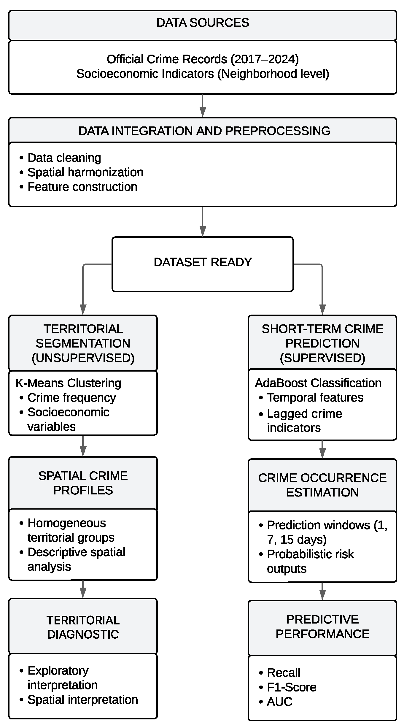
The methodological design of this study follows the Knowledge Discovery in Databases (KDD) framework, which provides a structured and iterative process for transforming raw data into actionable knowledge. Within this analytical setting, the proposed approach combines two complementary analytical components: territorial segmentation through unsupervised learning and short-term crime prediction through supervised classification. The complete workflow is summarized in Figure 1.

4.1. Data Integration and Preprocessing

The analysis begins with the integration of official crime records and contextual information at the colonia level. Crime data were obtained from administrative records compiled by public security institutions, while contextual variables were derived from official statistical sources. Both datasets were spatially harmonized to ensure consistency in geographic identifiers.

Preprocessing procedures included the elimination of duplicate and non-assignable records, standardization of colonia names, and removal of special characters to ensure compatibility across sources. Records corresponding to crime categories with incomplete temporal coverage were excluded to preserve the consistency of the analytical period. A unified date variable was constructed from year, month, and day fields to support subsequent feature engineering.

4.2. Feature Engineering

Temporal attributes include cyclical calendar variables such as day of the week and month of the year. To preserve temporal continuity (e.g., adjacency between Sunday and Monday or December and January), cyclical variables were encoded using sine and cosine transformations rather than independent categorical representations. In addition, cumulative and lag-based indicators were constructed to capture recent crime dynamics within each colonia

Short-term crime dynamics were captured through lag-based indicators computed over the previous 7 and 30 days, together with a cumulative crime intensity measure reflecting historical frequency within each neighborhood.

Formally, let $C_{i,t}$ denote the number of crime events observed in neighborhood i at time t. The lag-based indicators are defined as rolling sums over previous windows:

$$L_{i,t}^{\left(7\right)}=\sum _{k=1}^7{C}_{i,t-k}$$

(1)

$$L_{i,t}^{\left(30\right)}=\sum _{k=1}^{30}{C}_{i,t-k}$$

(2)

where $L_{i,t}^{\left(7\right)}$ and $L_{i,t}^{\left(30\right)}$ represent the total number of crime events occurring in the previous 7 and 30 days, respectively.

An initial specification included a 15-day lag variable; however, correlation analysis on the training subset (≤2021) revealed strong linear dependence between the 15-day and 30-day indicators. To prevent redundancy and improve numerical stability, the 15-day lag was removed from the final predictive specification.

The final temporal feature set therefore includes: (i) events in the previous 7 days, (ii) events in the previous 30 days.

Cyclical temporal variables were encoded using sine and cosine transformations to preserve their periodic structure. In this study, the cyclical variable x represents the calendar week index within the annual cycle ($W_t$), with period $T=52$. This encoding avoids artificial discontinuities that arise when cyclical variables are treated as ordinal values (e.g., the transition between week 52 and week 1).

$$sin\left(x\right)=sin\left({\displaystyle \frac{2\pi x}{T}}\right),$$

(3)

$$cos\left(x\right)=cos\left({\displaystyle \frac{2\pi x}{T}}\right).$$

(4)

This encoding allows the model to capture circular temporal proximity. Both sine and cosine transformations are required to represent the cyclical variable in a two-dimensional space, enabling the model to capture phase information. Although sine and cosine are phase-shifted functions, their joint use provides a complete and non-redundant representation of periodic behavior.

To capture long-term temporal progression, a linear time index was included:

$$D_t=t-t_0$$

(5)

where $t_0$ denotes the first observation date in the dataset. This variable captures monotonic temporal drift and long-term structural changes.

Seasonal structure was additionally represented using the calendar week index:

$$W_t\in \{1,2,\dots ,52\}$$

(6)

This variable serves as the basis for the cyclical encoding described above, where $x=W_t$ and $T=52$. To preserve periodic consistency, all observations were mapped to a 52-week annual cycle. In cases where calendar years included an additional week (week 53), these observations were reassigned to week 52.

Multicollinearity Assessment

To formally evaluate potential multicollinearity among temporal predictors, Pearson correlation coefficients and Variance Inflation Factors (VIF) were computed using exclusively the training subset (records up to 2021) to preserve chronological integrity.

The resulting correlation matrix showed moderate association between the 7-day and 30-day lag variables ($r=0.8497$). Although the correlation is relatively high, it remains below commonly accepted thresholds for problematic multicollinearity in predictive modeling.

In contrast, the 15-day lag variable exhibited a near-perfect linear correlation with the 30-day lag variable (r = 0.9742), indicating substantial redundancy. For this reason, the 15-day lag was excluded from the final model to reduce redundancy and mitigate potential multicollinearity effects.

Variance Inflation Factors were computed as:

$$VI{F}_i={\displaystyle \frac{1}{1-R_i^2}}$$

(7)

Table 2. Variance Inflation Factor (VIF) for temporal predictors (training subset ≤ 2021).

Variable	VIF
EVENTO_ULTIMOS_7_DIAS	3.61
EVENTO_ULTIMOS_30_DIAS	4.35
FRECUENCIA_ACUMULADA	1.59

reports the VIF values for the temporal predictors evaluated in the training subset.

The cumulative crime intensity variable is defined as the total number of crime events historically observed in each neighborhood:

$$F_i=\sum _{t=1}^T{C}_{i,t}$$

where $F_i$ represents the accumulated crime frequency for neighborhood i over the observation period.

While moderate multicollinearity is observed between the 7-day and 30-day lag variables, the accumulated frequency variable exhibits a substantially lower VIF, indicating limited redundancy across temporal predictors.

All VIF values remain below a conservative threshold of 5. While values above 10 are commonly considered indicative of serious multicollinearity [20], thresholds in the range of 5–10 are often treated as potentially problematic in applied settings [21]. In this context, adopting a threshold of 5 provides a stricter criterion to ensure limited multicollinearity among predictors.

Moderate correlation between the 7-day and 30-day lag variables is not expected to adversely affect model performance. Unlike linear regression models, AdaBoost employs sequential decision stumps (depth-1 trees) as weak learners. These univariate splits do not estimate simultaneous coefficients across correlated predictors. Therefore, multicollinearity is less likely to induce variance inflation or coefficient instability compared to parametric linear models.

Instead, correlated predictors may introduce redundancy but do not generate numerical singularities. The reported VIF values below 5 suggest that multicollinearity is not severe within the evaluated predictors. Empirical validation results across municipalities further demonstrate stable generalization without erratic variance patterns.

Contextual features include the type of urban settlement associated with each colonia and aggregate indicators reflecting the historical volume of crime. Together, these variables provide a structured representation of both short-term dynamics and longer-term crime intensity at the territorial level.

4.3. Spatial Segmentation Through Clustering

Territorial segmentation was performed using an unsupervised clustering approach to identify groups of colonias with similar crime-related characteristics. Clustering was conducted using the K-Means algorithm, selected for its efficiency and suitability for partitioning large spatial datasets. Prior to clustering, numerical variables were normalized to avoid scale effects.

The clustering feature space was restricted to four standardized variables: total crime frequency per neighborhood, marginalization index, total population, and percentage of population without basic education. The selected variables capture complementary dimensions of territorial structure related to crime concentration. The marginalization index reflects multidimensional socioeconomic deprivation, including housing conditions, access to basic services, and educational attainment. Total population accounts for the demographic scale of each colonia, while the percentage of population aged 15 and over without basic education serves as a proxy for educational vulnerability. Together, these variables provide a parsimonious representation of structural conditions associated with crime concentration. This restriction reduces multicollinearity across crime subcategories and enhances cross-municipal interpretability.

Table 3. Variables included in the clustering feature space and their analytical roles.

Variable	Description	Role in Clustering
Total crime frequency	Total number of crime events recorded per colonia	Crime intensity indicator
Marginalization index	Composite index reflecting socioeconomic deprivation	Structural socioeconomic condition
Total population	Total number of inhabitants per colonia	Demographic scale
Population without basic education (%)	Percentage of population aged 15 and over without completed basic education	Educational vulnerability indicator

summarizes the variables included in the clustering feature space, along with their definitions and analytical roles.

Similarity between observations was measured using the Euclidean distance after standardization, ensuring that all variables contribute comparably to distance calculations. Given two observations ${\mathbf{x}}_i$ and ${\mathbf{x}}_j$ described by p numerical attributes, the Euclidean distance is defined as:

$$d({\mathbf{x}}_i,{\mathbf{x}}_j)=\sqrt{\sum _{k=1}^p{(x_{ik}-x_{jk})}^2}.$$

(8)

The optimal number of clusters was determined using internal validation criteria. First, the elbow method was applied by examining the within-cluster sum of squares (WCSS) as a function of the number of clusters k. Formally, for a given partition with k clusters, the objective minimized by K-Means is:

$$\underset{C_1,\dots ,C_k}{min}\sum _{i=1}^k\sum _{{\mathbf{x}}_j\in C_i}{\parallel {\mathbf{x}}_j-{\mathit{\mu }}_i\parallel }^2,$$

(9)

where ${\mathit{\mu }}_i$ denotes the centroid of cluster $C_i$.

In addition, cluster quality was evaluated using the Davies–Bouldin index [22], defined as:

$$DB\left(k\right)={\displaystyle \frac{1}{k}}\sum _{i=1}^k\underset{j\ne i}{max}\left({\displaystyle \frac{S_i+S_j}{M_{ij}}}\right),$$

(10)

where $S_i$ represents the average intra-cluster dispersion of cluster i and $M_{ij}$ denotes the Euclidean distance between centroids of clusters i and j. Lower values of the Davies–Bouldin index indicate better cluster separation and compactness.

For each municipality, the optimal number of clusters was selected by solving the internal optimization problem:

$$k^{*}=arg\underset{k\in \{2,\dots ,10\}}{min}DB\left(k\right)$$

(11)

ensuring that cluster selection was driven by a formal internal validity criterion rather than exclusively by visual elbow inspection.

The selected number of clusters $k^{*}$ corresponds strictly to the configuration minimizing $DB\left(k\right)$ for each municipality.

The resulting clusters define a territorial typology that supports exploratory analysis and spatial interpretation. Importantly, cluster assignments were used exclusively for descriptive purposes and were not incorporated as predictors in the supervised classification models, ensuring a clear conceptual separation between segmentation and prediction.

This separation ensures that the predictive model focuses exclusively on temporal dynamics, preventing the introduction of static structural dependencies that may introduce bias in predictive performance under chronological validation.

To ensure robustness of the clustering results, the K-Means algorithm was executed using multiple random initializations (n_init = ‘auto’ in scikit-learn), which internally evaluates several centroid configurations. This reduces sensitivity to initialization and improves the stability of the resulting cluster assignments.

Additionally, cluster validity was assessed using the Davies–Bouldin index across evaluated configurations, supporting the reliability of the selected clustering solution.

4.4. Construction of Prospective Target Variables

Crime prediction was formulated as a binary classification problem. For each colonia and reference date, three independent prediction tasks were defined, each corresponding to a distinct forecasting horizon (1-day, 7-day, and 15-day windows).

Each task corresponds to an independent binary classification problem that models the probability of at least one crime event occurring within its respective future time window. This formulation enables short-term crime anticipation without relying on explicit time-series modeling, focusing instead on window-based event occurrence.

Table 4. Definition of prediction windows.

Window	Prediction Horizon	Target Definition
Short-term	1 day	Crime occurrence within next 24 h
Medium-term	7 days	Crime occurrence within next 7 days
Extended-term	15 days	Crime occurrence within next 15 days

presents the definition of the prediction windows used in the supervised classification task.

Formally, for each neighborhood and reference time t, the target variable $y_t$ is defined as:

$$y_t=\left\{\begin{array}{cc}1,\hfill & \mathrm{if}\mathrm{at}\mathrm{least}\mathrm{one}\mathrm{crime}\mathrm{event}\mathrm{occurs}\mathrm{in}(t,t+\Delta t],\hfill \\ 0,\hfill & \mathrm{otherwise},\hfill \end{array}\right.$$

(12)

where $\Delta t\in \{1,7,15\}$ days represents the prediction window.

4.5. Supervised Classification and Class Imbalance Handling

Supervised learning was implemented using the AdaBoost ensemble algorithm. AdaBoost iteratively combines weak learners and emphasizes misclassified observations, making it well suited for heterogeneous and imbalanced crime datasets. Separate models were independently trained for each prediction horizon, ensuring no cross-horizon dependency.

Formally, AdaBoost constructs an additive model of the form:

$$F_M\left(x\right)=\sum _{m=1}^M{\alpha }_m{h}_m\left(x\right),$$

(13)

where $h_m\left(x\right)$ denotes the m-th weak learner (decision stump), ${\alpha }_m$ is its associated weight, and M is the total number of boosting iterations.

At each iteration, sample weights are updated according to:

$$w_i^{(m+1)}=w_i^{\left(m\right)}exp\left(-{\alpha }_m{y}_i{h}_m\left(x_i\right)\right),$$

(14)

where $y_i\in \{-1,1\}$ represents the class label. The coefficient ${\alpha }_m$ is computed as:

$${\alpha }_m={\displaystyle \frac{1}{2}}ln\left({\displaystyle \frac{1-{\epsilon }_m}{{\epsilon }_m}}\right),$$

(15)

with ${\epsilon }_m$ denoting the weighted classification error of the m-th weak learner. This exponential loss minimization framework allows the ensemble to iteratively focus on previously misclassified observations while maintaining controlled model complexity.

Hyperparameter Selection and Final Model Configuration

An initial benchmarking phase was conducted to compare multiple classifiers (Logistic Regression, Random Forest, Support Vector Machine, XGBoost, AdaBoost, K-Nearest Neighbors, and Gradient Boosting) using GridSearchCV (scikit-learn, Python) with stratified five-fold cross-validation. The optimization criterion was recall, prioritizing the detection of true crime events due to the operational cost of false negatives.

Hyperparameter tuning was performed using grid search within a cross-validation framework (StratifiedKFold, $k=5$), optimizing recall as the primary evaluation metric. This procedure was applied across multiple candidate models during the benchmarking stage to ensure a fair and systematic comparison.

For AdaBoost, the parameter grid included $\mathrm{n}\_\mathrm{estimators}\in \{50,100,200\}$ and $\mathrm{learning}\_\mathrm{rate}\in \{0.01,0.1,1\}$. These values were selected to explore different levels of ensemble complexity and shrinkage intensity. In boosting frameworks, the number of estimators (M) and the learning rate ($\nu$) act as key regularization parameters, jointly controlling the bias–variance trade-off. Lower learning rates (shrinkage) typically improve generalization but require a larger number of estimators, while higher learning rates allow faster convergence but may increase the risk of overfitting. Therefore, evaluating combinations across these ranges enables a balanced exploration of model behavior [23,24]. This preliminary phase identified AdaBoost as one of the most stable models in terms of recall and standard deviation across municipalities and temporal windows.

The effect of these hyperparameter choices is reflected in the benchmarking results reported in

Table 5. Mean recall and standard deviation across prediction windows.

Model	Mean Recall	Std
SVM	0.801	0.033
AdaBoost	0.786	0.015
Logistic Regression	0.782	0.020
KNN	0.740	0.086
Gradient Boosting	0.712	0.097
Random Forest	0.651	0.110
XGBoost	0.635	0.198

. The evaluated configurations allowed the model to explore different bias–variance regimes, resulting in stable recall performance and the lowest inter-window variability (standard deviation) among the compared models. This empirical evidence provides support for the adequacy of the selected hyperparameter ranges in capturing stable predictive behavior across temporal horizons.

To ensure robustness across forecasting horizons, model performance was evaluated independently for the 1-day, 7-day, and 15-day windows. Mean recall and inter-window variability were computed for each classifier.

Although SVM achieved the highest mean recall, AdaBoost exhibited the lowest inter-window variability (standard deviation = 0.015), indicating superior stability across forecasting horizons. Given the operational objective of maintaining consistent detection performance under varying temporal windows, AdaBoost provided the best balance between high recall and minimal variance.

It is important to clarify that this benchmarking phase was conducted exclusively for model selection purposes. The temporal validation results presented in the Results section correspond solely to the chronologically validated configuration described below and were not obtained from shuffled cross-validation procedures.

The final model reported in the temporal validation section was trained under a strict chronological split (train ≤ 2021, validation = 2022, blind test ≥ 2023). In this configuration, AdaBoost was implemented with 100 weak learners (n_estimators = 100) and a learning rate of 0.05. The base learner corresponds to the default decision stump used in Scikit-Learn (DecisionTreeClassifier with max_depth = 1), ensuring low individual variance and improved ensemble generalization through boosting.

The final learning rate value (0.05) was selected as a conservative configuration within the explored range to improve generalization under chronological validation, as preliminary results indicated that lower shrinkage values provided more stable performance across temporal splits.

To address class imbalance, SMOTE was applied exclusively to the training subset after temporal splitting. The technique was implemented with default parameters (k_neighbors = 5, sampling_strategy = ‘auto’), where the minority class is oversampled until both classes reach equal representation in the training data.

This results in a balanced class distribution (approximately 1:1 ratio) in the training subset, while preserving the original distribution in validation and blind test periods to avoid temporal leakage.

Numerical variables were scaled using a robust normalization strategy based on the median and interquartile range. Non-ordinal categorical variables were encoded using one-hot encoding, while cyclical temporal variables were represented through sine–cosine transformations to preserve periodic structure.

4.6. Model Training and Evaluation

Model performance was evaluated using a chronological validation strategy to preserve the temporal structure of crime data. Given the forward-looking nature of crime prediction, the dataset was partitioned using an expanding-window approach: historical records from the initial period were used for training, the subsequent year (2022) was reserved for validation, and the most recent period (2023–2024) was treated as a blind test set. This design prevents information leakage and ensures that predictions are strictly prospective rather than retrospectively informed.

Evaluation metrics included accuracy, precision, recall, F1-score, and the area under the ROC curve (AUC). Given the operational relevance of crime anticipation, particular emphasis was placed on recall to minimize false negatives. Performance was assessed independently for each temporal horizon, allowing comparison of predictive behavior across short-term windows.

Given the operational relevance of minimizing undetected crime events, recall was prioritized as a key evaluation metric. Recall is defined as:

$$\mathrm{Recall}={\displaystyle \frac{TP}{TP+FN}},$$

(16)

where $TP$ denotes true positives and $FN$ false negatives.

Nevertheless, recall is not interpreted in isolation. To ensure a balanced evaluation, F1-score is also reported as a complementary metric, capturing the trade-off between detection capacity (recall) and false positive control (precision).

While recall is prioritized from an operational perspective, F1-score is used as the primary metric for comparative evaluation across municipalities.

5. Results

This section presents the results obtained from the two analytical components of the proposed approach: territorial segmentation using unsupervised clustering and short-term crime prediction using supervised machine learning. Results are reported using the best-performing configuration identified during the internal benchmarking phase described in Section 4.

5.1. Territorial Segmentation Results

Territorial segmentation was conducted using the K-Means algorithm, enabling the identification of homogeneous neighborhood groups based on crime incidence and socioeconomic characteristics. Clustering was performed independently for each municipality to capture localized spatial dynamics and avoid imposing a uniform clustering structure across the state.

Cluster quality was evaluated using the Davies–Bouldin index. Across the eleven municipalities analyzed, Davies–Bouldin values ranged from 0.032 to 0.829, indicating heterogeneous levels of intra-cluster compactness and centroid separation across local contexts. Lower values were observed in municipalities such as El Mante and Victoria, suggesting highly compact and well-separated cluster structures, whereas higher values in municipalities such as Nuevo Laredo reflect greater territorial complexity and structural heterogeneity.

Table 6. Territorial clustering results by municipality based on total crime frequency and socioeconomic indicators ($k^{*}$: denotes the optimal number of clusters).

Municipality	Optimal Clusters (${\mathit{k}}^{*}$)	Davies–Bouldin
Altamira	3	0.657
Ciudad Madero	2	0.493
El Mante	2	0.032
Matamoros	3	0.042
Nuevo Laredo	8	0.829
Reynosa	3	0.755
Río Bravo	2	0.275
San Fernando	6	0.441
Tampico	5	0.768
Valle Hermoso	2	0.047
Victoria	2	0.033

summarizes the optimal number of clusters selected for each municipality and the corresponding Davies–Bouldin index.

The resulting clusters provide an interpretable territorial diagnostic by revealing distinct spatial patterns of criminal activity. In several municipalities, a limited number of neighborhoods concentrate a disproportionately high number of crime events, while other clusters exhibit consistently low incidence levels despite adverse socioeconomic conditions. These results highlight the usefulness of territorial segmentation as a tool for spatial crime diagnosis and localized analysis.

Representative Cluster Profiling: Reynosa

To provide an interpretable illustration of the territorial segmentation process, we present the detailed cluster structure for Reynosa, where the optimal configuration was $k^{*}=3$ based on Davies–Bouldin minimization ($DB=0.765$). A total of 244 neighborhoods were included after spatial harmonization and data cleaning.

Table 7. Cluster profile for Reynosa ($k^{*}=3$).

Cluster	Total Crime	Marginalization	Population	No Basic Education	N
1	42.33	149.21	755.94	27.44	215
2	182.70	150.17	5089.48	24.17	23
3	682.83	149.05	2003.17	23.59	6

summarizes the average feature values per cluster.

The resulting structure reveals a highly asymmetric territorial configuration. Cluster 1 encompasses the majority of neighborhoods (88%), characterized by low crime incidence and relatively small population size. Cluster 2 contains a limited number of highly populated neighborhoods exhibiting intermediate crime intensity. In contrast, Cluster 3, composed of only six neighborhoods, concentrates extremely high crime levels, indicating strong spatial concentration effects.

Importantly, marginalization levels remain relatively stable across clusters, suggesting that crime differentiation in Reynosa is more strongly associated with demographic scale and localized concentration dynamics than with structural marginalization differences alone. This pattern illustrates the diagnostic value of clustering as a territorial characterization tool without introducing predictive dependency into the supervised modeling stage.

5.2. Temporal Predictive Validation Results

To evaluate predictive generalization under realistic temporal constraints, model performance was assessed using an expanding-window validation strategy. The training set included historical records up to 2021, the year 2022 was reserved for forward validation, and the period 2023–2024 was treated as a blind test set.

5.2.1. Class Distribution Analysis and Imbalance Structure

Before presenting predictive performance metrics, we examine the class distribution across temporal partitions in order to contextualize recall behavior and justify imbalance handling strategies.

Table 8. Class distribution across temporal partitions (Reynosa, 7-day window).

Period	N	Class 0 (%)	Class 1 (%)	Imbalance Ratio (0/1)
Train ≤ 2021	15,533	0.520	0.480	1.08
Validation 2022	2219	0.612	0.388	1.58
Blind ≥ 2023	4351	0.641	0.359	1.79

presents the class distribution for the selected case study (Reynosa, 7-day window).

The training subset exhibits near balance (48% positive class), whereas the validation and blind periods display progressively increasing imbalance ratios (1.58 and 1.79, respectively). This structural shift indicates that crime occurrence becomes relatively less frequent in the most recent periods, increasing classification difficulty under forward temporal validation.

The observed imbalance justifies the prioritization of recall as the principal evaluation metric, given the operational cost of false negatives in crime anticipation. Importantly, SMOTE was applied exclusively to the training subset, ensuring that synthetic balancing did not contaminate validation or blind partitions. Therefore, reported performance metrics reflect genuine predictive generalization under naturally imbalanced forward data rather than artificially balanced evaluation conditions.

5.2.2. Numerical Validation Example: Confusion Matrix and ROC Construction

To provide full transparency regarding metric computation, we present a numerical validation example using the 2022 forward validation set for Reynosa. The test partition contains $n=2219$ observations.

The resulting confusion matrix is:

$$\mathbf{C}=\left[\begin{array}{cc}1123& 236\\ 330& 530\end{array}\right]$$

(17)

where $TN=1123$, $FP=236$, $FN=330$, and $TP=530$.

Total observations:

$$N=1123+236+330+530=2219.$$

(18)

Performance metrics are computed as:

$$\mathrm{Accuracy}={\displaystyle \frac{TP+TN}{N}}={\displaystyle \frac{530+1123}{2219}}=0.7449$$

(19)

$$\mathrm{Precision}={\displaystyle \frac{TP}{TP+FP}}={\displaystyle \frac{530}{766}}=0.6919$$

(20)

$$\mathrm{Recall}={\displaystyle \frac{TP}{TP+FN}}={\displaystyle \frac{530}{860}}=0.6163$$

(21)

$$\mathrm{F}1=2{\displaystyle \frac{Precision·Recall}{Precision+Recall}}=0.6519$$

(22)

These values exactly coincide with the reported validation metrics, confirming internal computational consistency.

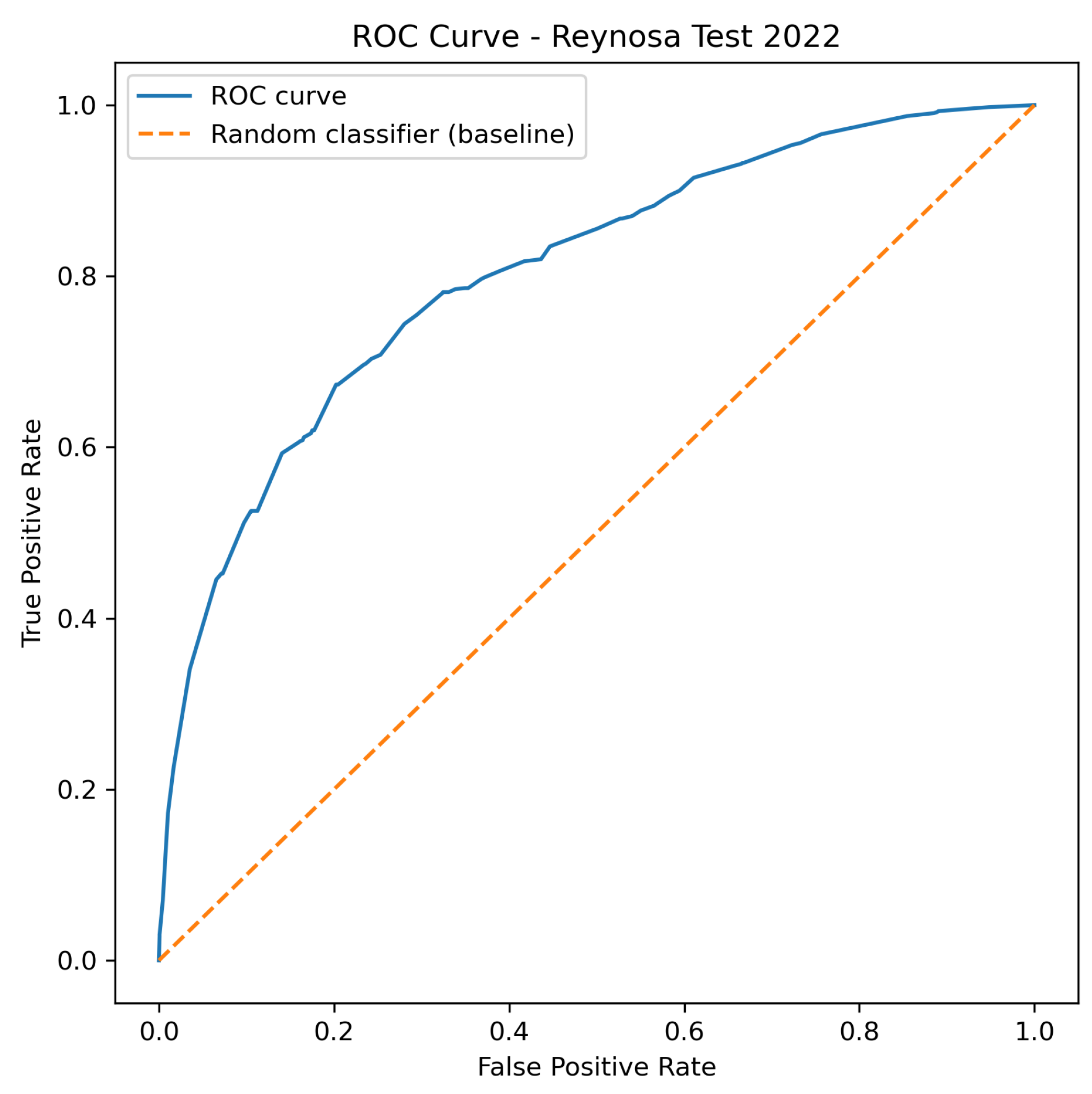
The ROC curve was constructed by varying the decision threshold $\tau \in [0,1]$ and computing:

$$\mathrm{TPR}\left(\tau \right)={\displaystyle \frac{TP\left(\tau \right)}{TP\left(\tau \right)+FN\left(\tau \right)}}$$

(23)

$$\mathrm{FPR}\left(\tau \right)={\displaystyle \frac{FP\left(\tau \right)}{FP\left(\tau \right)+TN\left(\tau \right)}}$$

(24)

The empirical AUC for the 2022 validation set equals $0.8031$, indicating strong discriminative capacity substantially above random classification ($AUC=0.5$).

Figure 2 presents the Receiver Operating Characteristic (ROC) curve for the 2022 validation set. The diagonal dashed line represents the performance of a random classifier and serves as a baseline for comparison. The ROC curve of the model lies substantially above this reference line, indicating strong discriminative ability. A higher true positive rate (TPR) for a given false positive rate (FPR) indicates that the model correctly identifies a larger proportion of actual crime events without proportionally increasing false alarms. This reflects a more favorable trade-off between sensitivity and specificity, which is desirable in crime prediction contexts where failing to detect true events (false negatives) carries a high operational cost.

To further investigate the contribution of individual predictors, feature importance was computed based on normalized importance weights derived from the trained AdaBoost ensemble. The results indicate that predictive performance is primarily driven by temporal intensity variables, particularly the 30-day lag (importance = 0.41), cumulative frequency (0.38), and long-term temporal progression (0.21).

Importantly, although lag-based variables dominate predictive contribution, the inclusion of additional temporal features contributes to improved stability across temporal partitions, as demonstrated in the baseline comparison analysis.

This result indicates that while lag-based variables capture the primary predictive signal, additional temporal features contribute to improved generalization under distributional shifts observed in forward temporal validation.

In contrast, cyclical calendar features (day-of-week and month encodings) and short-term lag (7 days) exhibit negligible contribution to the model. This suggests that crime occurrence is more strongly influenced by medium-term persistence and accumulated activity rather than short-term fluctuations or seasonal periodicity.

These findings support the robustness of the temporal feature design while confirming that lag-based variables capture the dominant predictive signal in the dataset.

5.2.3. Blind Temporal Generalization and Stability

To evaluate true forward generalization, the most recent period (2023–2024) was reserved as a blind test set, never exposed during training or model selection.

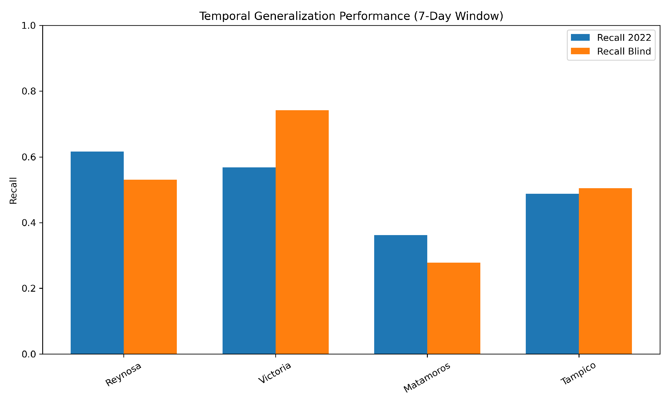
For Reynosa, recall in the 2022 validation year was 0.616, while blind recall decreased to 0.531, producing a temporal drift defined as:

$${\Delta }_{recall}=Recal{l}_{2022}-Recal{l}_{blind}=0.616-0.531=0.086$$

(25)

Although moderate drift is observed, the model preserves discriminative structure, with blind AUC remaining within acceptable operational thresholds (0.756).

Importantly, because SMOTE was applied exclusively to the training subset and chronological splitting was strictly enforced (train ≤ 2021, validation = 2022, blind ≥ 2023), these metrics are not affected by temporal leakage.

Across municipalities, the positive class proportion ranged between 35% and 48% in training partitions and decreased slightly in forward periods, reinforcing the need for imbalance-aware evaluation metrics. This structural variation further supports the use of recall as the primary operational indicator.

Table 9. Temporal validation results under expanding-window strategy.

Municipality	Recall 2022	Recall Blind	AUC Blind	Drift
Reynosa	0.616	0.531	0.756	0.086
Victoria	0.568	0.742	0.884	−0.174
Matamoros	0.362	0.278	0.777	0.084
Tampico	0.487	0.505	0.808	−0.018

summarizes representative results for selected municipalities with heterogeneous crime volumes, while Figure 3 illustrates the temporal generalization patterns.

The results show controlled variation between validation and blind periods rather than abrupt performance collapse. While moderate recall drift is observed in some municipalities, discrimination capacity measured through AUC remains stable, particularly in higher-volume urban contexts.

These findings indicate that short-term crime prediction remains feasible under strict temporal validation, although predictive strength varies according to local crime density and historical volatility.

The expanding-window design replicates the operational scenario faced by public security institutions: models are trained on historical data and deployed to predict future crime occurrence under potentially shifting distributions. The moderate recall drift observed between 2022 and the blind 2023–2024 period illustrates this realistic evaluation setting.

Accordingly, the validation strategy adopted here prioritizes methodological fidelity over optimistic performance estimates. The reported metrics therefore represent conservative yet operationally meaningful predictive capacity.

5.3. Unified Performance Across Municipalities

To provide a comprehensive evaluation of predictive performance across all analyzed municipalities,

Table 10. Unified predictive performance across all municipalities under chronological validation (7-day prediction window).

Municipality	Precision (2022)	Recall (2022)	F1 (2022)	Precision (Blind)	Recall (Blind)	F1 (Blind)
Altamira	0.531	0.722	0.612	0.443	0.788	0.567
Ciudad Madero	0.327	0.452	0.379	0.308	0.441	0.363
El Mante	0.639	0.765	0.696	0.724	0.856	0.784
Matamoros	0.500	0.362	0.420	0.403	0.278	0.329
Nuevo Laredo	0.390	0.485	0.432	0.219	0.184	0.200
Reynosa	0.692	0.616	0.652	0.612	0.531	0.568
Río Bravo	0.154	0.200	0.174	0.468	0.607	0.528
San Fernando	0.083	1.000	0.154	0.216	0.478	0.297
Tampico	0.624	0.487	0.547	0.601	0.505	0.549
Valle Hermoso	0.000	0.000	0.000	0.000	0.000	0.000
Victoria	0.761	0.568	0.650	0.761	0.742	0.752

reports Precision, Recall, and F1-score for both the validation period (2022) and the blind test period (2023–2024).

In this context, F1-score is used as the primary metric for cross-municipality comparison, as it balances recall and precision under varying class imbalance conditions.

Unlike the selected subset presented in Table 9, which highlights representative municipalities for interpretative clarity, this table includes the complete set of eleven municipalities to ensure full transparency and avoid selective reporting bias.

Performance variability across municipalities reflects differences in crime density, class imbalance, and temporal stability, rather than inconsistencies in model specification.

While Table 10 provides a comprehensive overview of predictive performance across all municipalities, notable heterogeneity is observed in model behavior.

In low-density contexts such as Valle Hermoso, the absence of positive instances in the validation period (2022) leads to zero precision, recall, and F1-score. This condition represents an extreme case of class sparsity where standard classification metrics become degenerate and non-informative, and therefore should be interpreted as a data limitation rather than a model performance indicator.

Conversely, municipalities such as San Fernando exhibit perfect recall (1.000) combined with very low precision, indicating systematic over-detection of crime events. This behavior is consistent with imbalance-sensitive learning under resampling strategies, where sensitivity is prioritized at the expense of specificity.

Intermediate cases, including Río Bravo and Nuevo Laredo, display variability between validation and blind periods, suggesting temporal instability and structural differences in crime dynamics across municipalities.

Overall, these results indicate that predictive performance is strongly conditioned by local crime prevalence, class imbalance, and temporal variability, reinforcing the need for context-specific interpretation rather than uniform performance expectations.

To assess the incremental value of the proposed feature set, the full model was compared against a baseline specification using only lagged variables (7- and 30-day windows).

Table 11. Baseline vs. Full Model Comparison (F1-score, Blind Period).

Municipality	F1 (Baseline)	F1 (Full)	Improvement
Altamira	0.627	0.567	−0.060
Ciudad Madero	0.355	0.363	+0.008
El Mante	0.761	0.784	+0.023
Matamoros	0.310	0.329	+0.019
Nuevo Laredo	0.131	0.200	+0.069
Reynosa	0.517	0.568	+0.051
Río Bravo	0.525	0.528	+0.003
San Fernando	0.244	0.297	+0.053
Tampico	0.527	0.549	+0.022
Valle Hermoso	0.000	0.000	0.000
Victoria	0.762	0.752	−0.010

reports F1-score differences under blind evaluation across all municipalities.

The comparison reveals that lag-based variables provide a strong predictive baseline across municipalities. In several cases (e.g., Altamira and Victoria), the baseline model achieves equal or slightly superior performance compared to the full specification.

Improvements are observed in municipalities such as El Mante, Reynosa, and Nuevo Laredo, where the full model yields higher F1-scores under blind evaluation. These gains are more evident in higher-density contexts, while differences remain marginal in low-density environments.

These results indicate that the contribution of the full model is context-dependent rather than universal. In low-density or highly stable environments, lagged variables alone capture a substantial portion of the predictive signal. In contrast, in municipalities with higher crime intensity and temporal variability, the inclusion of additional temporal features contributes to improved generalization.

Overall, the findings suggest that while lag-based features provide a strong baseline, increased feature complexity yields measurable benefits primarily under conditions of higher variability, supporting a nuanced interpretation of model performance across heterogeneous urban settings.

6. Discussion

The results obtained indicate the usefulness of addressing crime analysis through a modular analytical perspective that combines territorial segmentation and temporal prediction while maintaining a clear conceptual separation between both components. Clustering-based segmentation revealed differentiated spatial patterns across municipalities, reflecting the territorial heterogeneity of crime dynamics in the state of Tamaulipas. The observed variability in Davies–Bouldin index values indicates that the spatial structure of crime is not uniform and is strongly influenced by local conditions, supporting the relevance of intra-urban scale analysis.

Because cluster selection was formally determined through minimization of the Davies–Bouldin index under a fixed feature specification, the observed variability across municipalities reflects genuine territorial structural differences rather than differences in model configuration. The decision to perform clustering independently for each municipality is motivated by the objective of preserving local spatial structure and avoiding artificial homogenization across territorially heterogeneous contexts. A global clustering approach would impose a shared feature space that may obscure locally relevant patterns, particularly in regions with substantial variation in crime dynamics and urban scale. From a territorial perspective, the identified clusters show that criminal activity tends to concentrate in a limited number of neighborhoods within each municipality, while extensive areas exhibit consistently low incidence levels. This pattern is consistent with findings reported in spatial criminology studies and supports the use of unsupervised clustering as a diagnostic tool for territorial analysis. Rather than providing causal explanations, the resulting spatial profiles offer a descriptive foundation that facilitates exploratory analysis and supports differentiated decision-making in public security contexts.

It is important to note that clustering validation is based on internal criteria (Davies–Bouldin index), as no external ground truth is available for territorial typologies. Therefore, clustering results should be interpreted as descriptive rather than predictive structures.

Regarding the predictive component, performance under chronological validation demonstrates that short-term crime anticipation is feasible but context-dependent. Recall values vary across municipalities, reflecting differences in crime density, temporal volatility, and historical stability. Importantly, the absence of abrupt degradation between validation (2022) and blind (2023–2024) periods indicates context-dependent generalization under forward-looking evaluation. While moderate recall drift is observed in certain municipalities, discrimination capacity measured through AUC remains comparatively stable in higher-volume urban contexts. These findings suggest that predictive reliability is influenced by local structural characteristics rather than purely algorithmic performance.

In particular, performance variability is associated with differences in crime density, class imbalance, and temporal stability across municipalities. Low-density contexts tend to produce unstable or degenerate classification outcomes, while higher-density urban environments allow for more consistent predictive behavior.

A key methodological decision in the proposed modular framework is the explicit separation between territorial segmentation and predictive modeling. Cluster labels were not incorporated as explanatory variables in the supervised model, avoiding potential issues related to spatial dependence and overfitting. This design allows each analytical component to serve a distinct purpose: spatial segmentation enhances contextual understanding and interpretability, while supervised prediction focuses on operational anticipation of crime events.

Importantly, the separation between spatial and temporal components reflects a deliberate modeling choice aimed at improving interpretability and diagnostic clarity. This study does not evaluate whether such separation is methodologically preferable to fully integrated spatio-temporal models. Instead, the results indicate that predictive performance is strongly influenced by lag-based temporal dynamics, and that additional features provide context-dependent improvements. Future research should explicitly compare modular and integrated modeling strategies under consistent validation frameworks.

The municipality-specific clustering strategy adopted in this study was not evaluated against a global clustering alternative and should be interpreted as a context-sensitive analytical choice.

By maintaining methodological independence between components, the proposed approach enables a clearer distinction between persistent territorial patterns and dynamic crime fluctuations. This allows for a more interpretable assessment of predictive behavior and helps identify the conditions under which additional model complexity contributes to performance improvements.

Despite these strengths, several limitations should be acknowledged. First, the results depend on the quality and consistency of administrative crime records, which may be affected by underreporting or changes in data collection practices. Second, the use of internal validation metrics for clustering constrains direct comparison with alternative approaches based on external validation. Finally, the predictive model focuses on aggregated crime events without distinguishing between specific crime types (e.g., violent vs. property crimes). This simplification may obscure heterogeneous temporal dynamics across crime categories and represents a relevant direction for future research.

Overall, the findings support the relevance of the proposed analytical approach for crime analysis and short-term anticipation. By combining spatial interpretability and predictive capability through complementary analytical components, the approach provides a flexible and replicable solution for territorially heterogeneous contexts.

Importantly, the conservative performance estimates reported in this study reflect realistic deployment conditions rather than optimistic cross-validated interpolation, supporting the practical relevance of the proposed approach.

7. Conclusions and Future Work

This study presents a modular spatial–temporal approach for crime analysis, combining territorial segmentation through clustering and short-term prediction using supervised machine learning under a modular design.

The results show that spatial clustering captures intra-urban heterogeneity, providing a descriptive diagnostic of neighborhood-level crime patterns. The predictive model exhibits stable performance under strict chronological validation, with F1-score providing a balanced assessment between detection capacity and false positives. The findings indicate that recent crime dynamics, particularly lag-based variables, account for a substantial portion of predictive performance, while additional temporal features contribute to improved stability in specific urban contexts.

Importantly, predictive performance varies across municipalities, reflecting differences in crime density, class imbalance, and temporal regularity. These results highlight that model performance is context-dependent rather than uniform across territories and remains sensitive to local structural conditions.

Overall, the proposed approach provides a replicable and context-aware analytical approach for spatially differentiated crime risk estimation, combining territorial interpretation with forward-looking prediction without introducing structural dependencies between components. The approach should be interpreted as an applied modular strategy rather than a generalized spatio-temporal modeling framework.

Future research may explore alternative modeling strategies, including integrated or hierarchical approaches where spatial and temporal components are jointly modeled under different assumptions. Additionally, spatial cross-validation schemes and explainability techniques (e.g., SHAP-based attribution) may further enhance interpretability under strict chronological validation.