Article

A Second-Order Nonstandard Finite Difference Method for a Malaria Propagation Model with Control


by
Calisto B. Marime
* and
Justin B. Munyakazi
Department of Mathematics and Applied Mathematics, University of the Western Cape, Private Bag X17, Bellville 7535, South Africa
*
Author to whom correspondence should be addressed.
AppliedMath 2026, 6(3), 36; https://doi.org/10.3390/appliedmath6030036
Submission received: 16 August 2025 / Revised: 29 August 2025 / Accepted: 2 September 2025 / Published: 2 March 2026

Abstract

Standard numerical methods such as Runge–Kutta and Euler methods have been widely used to approximate solutions to nonlinear systems. These methods converge to the solution only for small step sizes; for larger time steps, they generally generate spurious or chaotic solutions. In this paper, we consider a malaria propagation model with control for which we construct a second-order nonstandard finite difference scheme that preserves the important mathematical properties of the continuous model, which are positivity, boundedness, and stability of solutions irrespective of the step size. Moreover, we show that the equilibrium points of the discrete model are the same as those of the continuous model. By applying the double mesh principle, we provide evidence that the second-order NSFD scheme approximates the true solution with small errors. Theoretical assertions and numerical results show the advantages of the developed second-order nonstandard finite difference method.

1. Introduction

In the fields of epidemiology, engineering, and other applied sciences, many situations are modeled using ordinary differential equations (ODEs). Some of the dynamical processes lead to highly nonlinear systems of ODEs. Due to the nonlinearity of the systems, finding analytical solutions proves to be a complicated exercise. In an attempt to approximate the solutions, several numerical methods have been employed by numerous researchers (see, for example, [1,2,3]). Some numerical methods generate inaccurate or meaningless solutions (see [4,5]). Mickens in [6] proposed a methodology to overcome drawbacks faced by standard numerical methods such as the Euler and Runge–Kutta methods. To this day, nonstandard finite difference (NSFD) schemes have been widely utilized in all fields of applied sciences and proved to be the most powerful numerical tool, with many advantages over standard finite difference (SFD) schemes (see, for example, [7,8,9,10,11]). Recently, high-order NSFD schemes have drawn the attention of many scholars (see [10,12,13]).
The second-order modified nonstandard theta method for one-dimensional autonomous differential equations in [13] partially resolves the contradiction between high-order NSFD accuracy and dynamical consistency. The scheme preserves local asymptotic stability and fails to be elementary stable even though it is second-order accurate. However, Hoang in [12] developed a second-order NSFD method for solving one-dimensional autonomous dynamical systems that preserves positivity of solutions and resolves the contradiction between high-order accuracy and dynamic consistency. Furthermore, Hoang in [14] developed third- and fourth-order NSFD methods for a one-dimensional system that preserves positivity and asymptotic stability. The obtained results have partially resolved the contradiction between the dynamic consistency and the high-order accuracy of the NSFD schemes. A stable numerical framework for analyzing dynamic crack propagation over extended time intervals was studied in [15]. The framework combines the Krylov Deferred Correction (KDC) method for temporal discretization with the Generalized Finite Difference Method (GFDM) for spatial discretization. The numerical results show reasonably consistent errors in dynamic simulations over a long period, regardless of the step size.
The second-order NSFD technique developed in [16] preserves the positivity, local asymptotic stability, and global asymptotic stability of a general single-species model. Newly proposed NSFD schemes are not only convergent of order two but are also dynamically consistent with the model under study (see [9,10]). This leads to advancements in more accurate numerical solutions of the continuous models. Two new classes of second-order modified NSFD explicit Euler and Runge–Kutta methods were developed in [17] for multi-dimensional autonomous dynamical systems. The scheme proved to be convergent of order two and elementary stable only for small time steps.
Standard numerical methods require a small time step for accuracy and stability, which is problematic for long simulations. Using small step sizes over long periods incurs high computational costs, making the standard schemes less efficient over extended horizons. This presents a gap in the numerical analysis of malaria dynamics, which requires long-term numerical integration.
NSFD methods are a serious alternative to standard numerical methods, as they are designed to preserve the qualitative features of the underlying systems regardless of the step size. In this work, we present a first-order NSFD scheme that is dynamically consistent with the continuous malaria propagation model in [18]. The convergence analysis of this scheme is similar to that of [11]. Also, we construct a second-order NSFD scheme for the same malaria propagation model. We prove that this scheme is also dynamically consistent and demonstrate its superiority vis-a-vis the first-order scheme in terms of accuracy, regardless of the step size. This work surely contributes to the broader effort of improving numerical tools for epidemiological modeling, with the ultimate goal of providing reliable solutions to inform disease control policies.
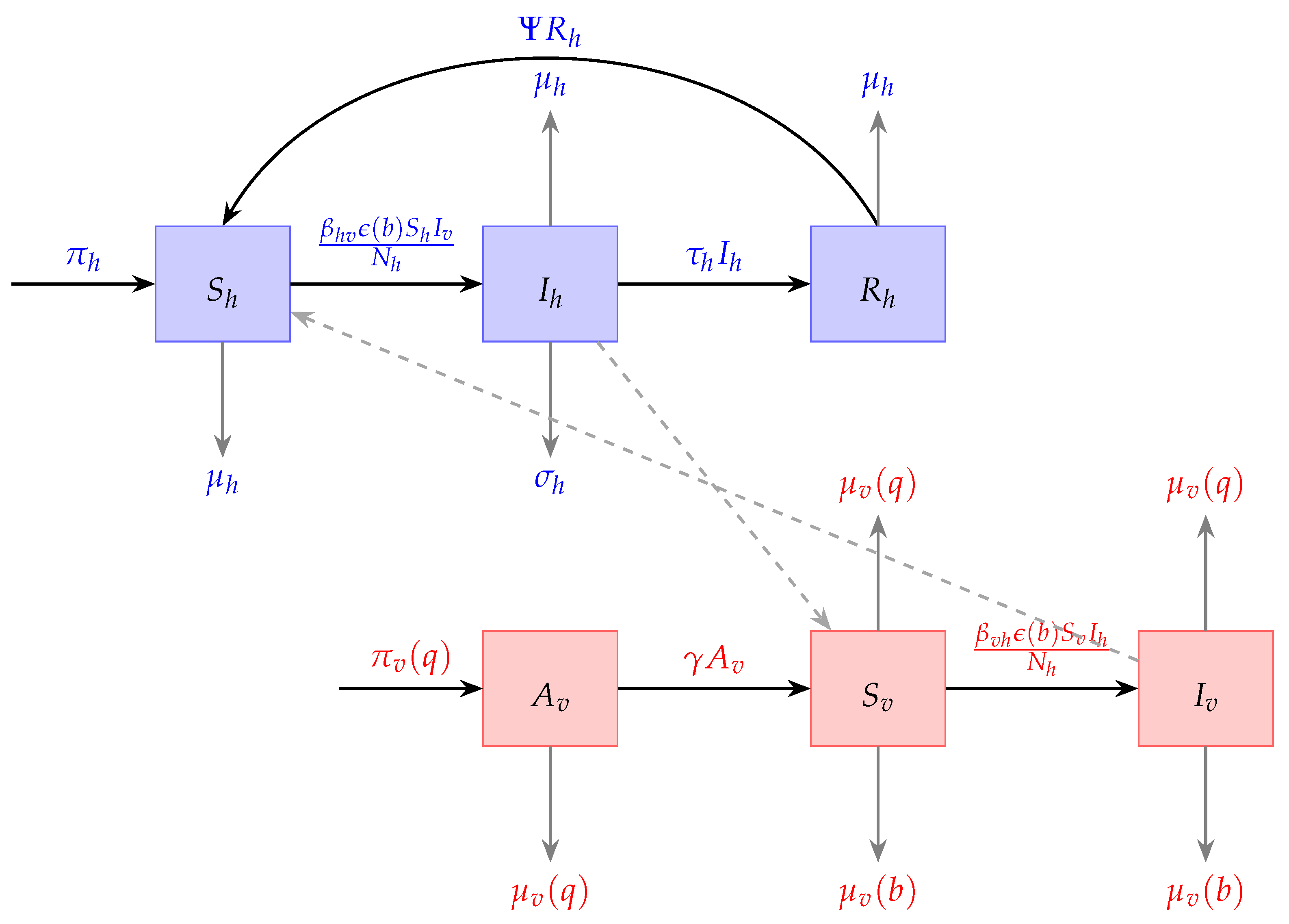
In the continuous model considered here, the human population is divided into susceptible humans ( S h ) , infected humans ( I h ) , and recovered humans ( R h ) , and the vector population is partitioned into immature mosquitoes ( A v ) , susceptible mosquitoes ( S v ) , and infected mosquitoes ( I v ) . Flow diagram is show in Figure 1.
The model is given by
d S h ( t ) d t = π h + Ψ R h ( t ) β h v ϵ ( b ) I v ( t ) S h ( t ) N h ( t ) μ h S h ( t ) d I h ( t ) d t = β h v ϵ ( b ) I v ( t ) S h ( t ) N h ( t ) ( τ h + μ h + σ h ) I h ( t ) d R h ( t ) d t = τ h I h ( t ) ( Ψ + μ h ) R h ( t ) d A v ( t ) d t = π v ( q ) ( γ v + μ v ( q ) ) A v ( t ) d S v ( t ) d t = γ v A v ( t ) β v h ϵ ( b ) I h ( t ) S v ( t ) N h ( t ) ( μ v ( b ) + μ v ( q ) ) S v ( t ) d I v ( t ) d t = β v h ϵ ( b ) I h ( t ) S v ( t ) N h ( t ) ( μ v ( b ) + μ v ( q ) ) I v ( t ) ,
with initial conditions
S h ( 0 ) = S 0 h > 0 , I h ( 0 ) = I 0 h 0 , R h ( 0 ) = R 0 h 0 A v ( 0 ) = A 0 v > 0 , S v ( 0 ) = S 0 v > 0 , I v ( 0 ) = I 0 v 0 ,
where π h and γ v are the recruitment rates for humans and mosquitoes in the susceptible class. After mosquito bites at a rate ϵ ( b ) , humans and mosquitoes move from the susceptible class to the infectious class at a rate β h v ϵ ( b ) I v N h and β v h ϵ ( b ) I h N h , respectively. In each compartment, the population is reduced by natural death at a rate of μ h for humans and μ v for mosquitoes. The mortality rate of mosquitoes due to treated nets and insecticide spray is given by μ v ( b ) and μ v ( q ) . The parameters μ v ( b ) and μ v ( q ) are treated as constants, representing average intervention levels. Moreover, induced death reduces the infected humans at a rate σ h . Infected humans are transferred to the recovery class at a rate τ h , and after some time, individuals lose immunity and become susceptible again at a rate Ψ . Immature mosquitoes are generated by egg deposition at a rate π v ( q ) and reduced by maturation of immature mosquitoes at a rate γ v .
The disease-free equilibrium (DFE) is given by
ϕ 0 = π h μ h , 0 , 0 , π v ( q ) γ v + μ v ( q ) , γ v π v ( q ) ( γ v + μ v ( q ) ) ( μ v ( b ) + μ v ( q ) ) , 0 ,
and the unique endemic equilibrium (EE) ϕ * exists if and only if the basic reproduction number R 0 > 1 , where
R 0 = β h v β v h γ v π v ( q ) μ h ϵ 2 ( b ) π h ( τ h + μ h + σ h ) ( γ h + μ v ( q ) ) ( μ v ( b ) + μ v ( q ) ) 2 ,
with
ϕ * = ( S h * , I h * , R h * , A v * , S v * , I v * ) ,
and
S h * = π h k 1 k 2 k 1 k 2 [ Λ h * ( b ) + μ h ] τ h Ψ Λ h * ( b ) , A v * = π ( q ) k 3 , I h * = Λ h * ( b ) π h k 2 k 1 k 2 [ Λ h * ( b ) + μ h ] τ h Ψ Λ h * ( b ) , S v * = γ v π v ( q ) k 3 [ Λ h * ( b ) + k 4 ] , R h * = Λ h * ( b ) τ h π h k 1 k 2 [ Λ h * ( b ) + μ h ] τ h Ψ Λ h * ( b ) , I v * = Λ v * ( b ) γ v π v ( q ) k 3 k 4 [ Λ v * ( b ) + k 4 ] ,
where
Λ h * ( b ) = β h v ϵ ( b ) I v * S h * N h * , Λ v * ( b ) = β v h ϵ ( b ) I h * S v * N h * , k 1 = τ h + μ h + σ h , k 2 = Ψ + μ h , k 3 = γ v + μ v ( q ) , k 4 = μ v ( b ) + μ v ( q ) .
We refer interested readers to [18] for more details on the model (1).
The structure of this paper is as follows: In Section 2, we construct the first-order NSFD (1NSFD) scheme and the second-order NSFD (2NSFD) method and prove the positivity and boundedness and determine the stability of the scheme. Moreover, we prove the order of convergence. In Section 3, we perform numerical simulations. In Section 4, we provide some concluding remarks on our work.

2. Construction of the NSFD Methods

We construct the first-order NSFD method and the second-order NSFD scheme for the continuous model (1).

2.1. Presentation of the First-Order NSFD Method

We consider the following uniform subdivision of the finite interval [ 0 , T e n d ] :
0 = t 0 < t 1 < < t N 1 < t N = T ,
where Δ t = t k t k 1 for 1 k N .
To approximate (1), a finite difference method can be expressed as (see [19,20])
D h ( X k ) = F h ( f : X k ) ,
where in the continuous model (1), D h ( X k ) d d t ( S h , I h , R h , A v , S v , I v ) T t = t k , t k = t 0 + k ( Δ t ) , where Δ t > 0 is the step size and F h ( f : X k ) approximates the right-hand side of the continuous model (1). The following definitions are important in the construction of the NSFD scheme.
Definition 1.
The finite difference method (1) is called positive if for any value of the step size Δ t , and X 0 R + 6 , its solutions remain positive, i.e., X k R + 6 for all k N [20].
Definition 2.
The finite difference method (5) is called elementary stable, if, for any value of the step size Δ t , its fixed point E 0 is the same as the equilibria of the differential system (1) and the local stability properties of each E 0 are same for both the differential system and the difference method [20].
Definition 3.
The one-step finite difference method (5) for solving model (1) is an NSFD if at least one of the following conditions is satisfied [11,21]:
  • D h ( X k ) = ( X k + 1 X k ) / ϕ ( Δ t ) , where ϕ ( Δ t ) = Δ t + O ( Δ t 2 ) is a non-negative function and is called the nonstandard denominator function.
  • The nonlinear terms are approximated non-locally, for example S h 2 ( t k ) S h k S h k + 1 .
Applying the NSFD framework above, the continuous-time model (1) is discretized as follows:
S h k + 1 S h k ϕ h ( Δ t ) = π h + Ψ R h k β h v ϵ ( b ) I v k S h k + 1 N h k μ h S h k + 1 , I h k + 1 I h k ϕ h ( Δ t ) = β h v ϵ ( b ) I v k S h k N h k ( τ h + μ h + σ h ) I h k + 1 , R h k + 1 R h k ϕ h ( Δ t ) = τ h I h k ( Ψ + μ h ) R h k + 1 , A v k + 1 A v k ϕ v ( Δ t ) = π v ( q ) ( γ v + μ v ( q ) ) A v k + 1 , S v k + 1 S v k ϕ v ( Δ t ) = γ v A v β v h ϵ ( b ) I h k S v k + 1 N h k ( μ v ( b ) + μ v ( q ) ) S v k + 1 , I v k + 1 I v k ϕ v ( Δ t ) = β v h ϵ ( b ) I h k S v k N h k ( μ v ( b ) + μ v ( q ) ) I v k + 1 ,
where ϕ h ( Δ t ) and ϕ v ( Δ t ) are the denominator functions for humans and mosquitoes, respectively. The scheme (6) depends on the step size and is first-order-convergent. Following the ideas of [11], it can be shown that the scheme above is dynamically consistent with the continuous system (1). However, the question of accuracy arises. It appears natural to couple dynamical consistency with fast convergence. Below, we propose another NSFD scheme with the aim of attaining a faster convergence while conserving the dynamical consistency.

2.2. Presentation of the Second-Order NSFD Method

Following Hoang’s ideas [10,12], the continuous model (1) is descretized as
S h k + 1 S h k ϕ 1 ( Δ t , S h k , R h k , I v k ) = π h + Ψ R h k β h v ϵ ( b ) I v k S h k + 1 N h k μ h S h k + 1 + θ 1 S h k θ 1 S h k + 1 , I h k + 1 I h k ϕ 2 ( Δ t , S h k , I h k , I v k ) = β h v ϵ ( b ) I v k S h k N h k ( τ h + μ h + σ h ) I h k + 1 + θ 2 I h k θ 2 I h k + 1 , R h k + 1 R h k ϕ 3 ( Δ t , I h k , R h k ) = τ h I h k ( Ψ + μ h ) R h k + 1 + θ 3 R h k θ 3 R h k + 1 , A v k + 1 A v k ϕ 4 ( Δ t , A v ) = π v ( q ) ( γ v + μ v ( q ) ) A v k + 1 + θ 4 A v k θ 4 A v k + 1 , S v k + 1 S v k ϕ 5 ( Δ t , I h k , A v k , S v k ) = γ v A v β v h ϵ ( b ) I h k S v k + 1 N h k ( μ v ( b ) + μ v ( q ) ) S v k + 1 + θ 5 S v k θ 5 S v k + 1 , I v k + 1 I v k ϕ 6 ( Δ t , I h k , S v k , I v k ) = β v h ϵ ( b ) I h k S v k N h k ( μ v ( b ) + μ v ( q ) ) I v k + 1 + θ 6 I v k θ 6 I v k + 1 .
where ϕ i ( Δ t , S h k , I h k , R h k , A v k , S v k , I v k ) = Δ t + O ( Δ t 2 ) as Δ t 0 ( i = 1 , 2 , 3 , 4 , 5 , 6 ) is the nonstandard denominator function and θ i ( i = 1 , 2 , 3 , 4 , 5 , 6 ) is a real number that represents weights. The scheme (7) depends iteratively on the solution.
Remark 1.
It is important to observe that the denominator functions ϕ h and ϕ v in (6) depend only on the step size Δ t . However, in the second-order NSFD scheme (7), the denominator function ϕ i depends on both the step size and iteratively on the state variables. Therefore, it must be recalculated at every time step and for every population compartment. The denominator functions ϕ i ( Δ t , S h k , I h k , R h k , A v k , S v k , I v k ) guarantee convergence of the scheme (7), while the weights ( θ i ) facilitate dynamic consistency. Although we treated μ v ( b ) and μ v ( q ) as constants, they can be generalized to time-dependent functions. The second-order NSFD scheme accommodates such time-varying functions by evaluating the control-dependent terms at each discrete step while maintaining the qualitative properties of the continuous model.

2.3. Qualitative Properties of the NSFD Scheme (7)

In this subsection, we prove the positivity and boundedness of solutions. For simplicity, in some instances, we omit arguments of the denominator functions.
Theorem 1.
The positivity of the continuous model (1) is conserved for any given step size whenever θ i 0 by the NSFD scheme (7).
Proof. 
The scheme (7) can be rewritten in the following explicit form:
S h k + 1 = S h k + ϕ 1 ( π h + Ψ R h k + θ S h k ) 1 + ϕ 1 β h v ϵ ( b ) I v k N h k + μ h + θ 1 , I h k + 1 = I h k + ϕ 2 β h v ϵ ( b ) I v k S h k N h k + θ I h k 1 + ϕ 2 ( τ h + μ h + σ h + θ 2 ) , R h k + 1 = R h k + ϕ 3 ( τ h I h k + θ R h k ) 1 + ϕ 3 ( Ψ + μ h + θ 3 ) , A v k + 1 = A v k + ϕ 4 ( π v ( q ) + θ A v k ) 1 + ϕ 4 ( γ v + μ v ( q ) + θ 4 ) , S v k + 1 = S v k + ϕ 5 ( γ v A v + θ S v k ) 1 + ϕ 5 β v h ϵ ( b ) I h k N h k + μ v ( b ) + μ v ( q ) + θ 5 , I v k + 1 = I v k + ϕ 6 β v h ϵ ( b ) I h k S v k N h k + θ 6 I v k 1 + ϕ 6 ( μ v ( b ) + μ v ( q ) + θ 6 ) .
Since all parameters in the system (8) are positive, it is clear that if
S h k , I h k , R h k , A v k , S v k , I v k 0
then
S h k + 1 , I h k + 1 , R h k + 1 , A v k + 1 , S v k + 1 , I v k + 1 0
holds unconditionally for all state variables. This concludes the proof. □
Theorem 2.
The NSFD scheme defines the discrete dynamical system (7) on
D = ( S h k , I h k , R h k , A v k , S v k , I v k ) : 0 S h k + I h k + R h k π h μ h , a n d 0 A v k + S v k + I v k π v ( q ) μ v .
Proof. 
Let us suppose that N h k = S h k + I h k + R h k and N v k = A v k + S v k + I v k ; then from (7) we have
N h k + 1 N h k ϕ h ( Δ t , S h k , I h k , R h k ) = π h μ h N h k + 1 σ I h k + θ h N h k θ h N h k + 1 , N v k + 1 N v k ϕ v ( Δ t , A v k , S v k , I v k ) = π v ( q ) μ v N v k + 1 μ v ( b ) A v k + θ v N v k θ v N v k + 1 .
From (10), we have
N h k + 1 = N h k ( 1 + ϕ h θ h ) 1 + ϕ h ( μ h + θ 1 ) + ϕ h π h 1 + ϕ h ( μ h + θ h ) ϕ h σ h I h k 1 + ϕ h ( μ h + θ h ) , N v k + 1 = N v k ( 1 + ϕ v θ v ) 1 + ϕ v ( μ v + θ v ) + ϕ v π v ( q ) 1 + ϕ v ( μ v + θ v ) ϕ v μ v ( b ) A v k 1 + ϕ v ( μ v + θ v ) .
From the first equation of (11), we have
N h k + 1 N h k ( 1 + ϕ h θ h ) 1 + ϕ h ( μ h + θ h ) + ϕ h π h 1 + ϕ h ( μ h + θ h ) 1 + ϕ h θ h 1 + ϕ h ( μ h + θ h ) ( 1 + ϕ h θ h ) N h k 1 1 + ϕ h ( μ h + θ h ) + ϕ h π h 1 + ϕ ( μ h + θ h ) + ϕ h π h 1 + ϕ h ( μ h + θ h ) = 1 + ϕ h θ h 1 + ϕ h ( μ h + θ h ) 2 N h k 1 + ϕ h π h 1 + ϕ h ( μ h + θ h ) 1 + ϕ h θ h 1 + ϕ h ( μ h + θ h ) + 1 1 + ϕ h θ h 1 + ϕ h ( μ h + θ h ) k + 1 N h 0 + ϕ h π h 1 + ϕ h ( μ h + θ h ) j = 0 k 1 + ϕ h θ h 1 + ϕ h ( μ h + θ h ) j = 1 + ϕ h θ h 1 + ϕ h ( μ h + θ h ) k + 1 N h 0 + ϕ h π h 1 + ϕ h ( μ h + θ h ) 1 1 + ϕ h θ h 1 + ϕ h ( μ h + θ h ) k + 1 1 1 + ϕ h θ h 1 + ϕ h ( μ h + θ h ) .
As k , we have lim k N h k π h μ h . Likewise, in the second equation of (11), N v k π v ( q ) μ v as k . The solutions for the human population and the mosquito population remain bounded in the region D. This completes the proof. □
Note 1.
In (12), the notion of geometric series has been utilized. For any given step size,   N h k  and  N v k  are bounded.

2.4. Stability of the NSFD Method

We will show that DFE is locally asymptotically stable for the NSFD scheme (7).
Theorem 3.
The NSFD scheme (7) is elementary stable for all step sizes whenever θ i 0 .
Proof. 
Firstly, we rewrite the scheme (8) as
S h k + 1 = S h k + ϕ 1 ( Δ t , S h k , R h k , I v k ) F 1 k ( S h k , R h k , I v k ) 1 + ϕ 1 ( Δ t , S h k , R h k , I v k ) β h v ϵ ( b ) I v k N h k + μ h + θ 1 , I h k + 1 = I h k + ϕ 2 ( Δ t , S h k , I h k , I v k ) F 2 k ( S h k , I h k , I v k ) 1 + ϕ 2 ( Δ t , S h k , I h k , I v k ) ( τ h + μ h + σ h + θ 2 ) , R h k + 1 = R h k + ϕ 3 ( Δ t , I h k , R h k ) F 3 k ( I h k , R h k ) 1 + ϕ 3 ( Ψ + μ h + θ 3 ) , A v k + 1 = A v k + ϕ 4 ( Δ t , A v ) F 4 ( A v ) 1 + ϕ 4 ( Δ t , A v ) ( γ v + μ v ( q ) + θ 4 ) , S v k + 1 = S v k + ϕ 5 ( Δ t , I h k , A v k , S v k ) F 5 ( I h k , A v k , S v k ) 1 + ϕ 5 β v h ϵ ( b ) I h k N h k + μ v ( b ) + μ v ( q ) + θ 5 , I v k + 1 = I v k + ϕ 6 ( Δ t , I h k , S v k , I v K ) F 6 k ( I h k , S v k , I v K ) 1 + ϕ 6 ( Δ t , I h k , S v k , I v K ) ( μ v ( b ) + μ v ( q ) + θ 6 ) ,
where
F 1 k ( S h k , R h k , I v k ) = π h + Ψ R h k β h v ϵ ( b ) I v k S h k N h k μ h S h k , F 2 k ( S h k , I h k , I v k ) = β h v ϵ ( b ) I v k S h k N h k ( τ h + μ h + σ h ) I h k , F 3 k ( I h k , R h k ) = τ h I h k ( Ψ + μ h ) R h k , F 4 k ( A v ) = π v ( q ) ( γ v + μ v ( q ) ) A v k , F 5 k ( I h k , A v k , S v k ) = γ v A v k β v h ϵ ( b ) I h k S v k N h k ( μ v ( b ) + μ v ( q ) ) S v k , F 6 k ( I h k , S v k , I v K ) = β v h ϵ ( b ) I h k S v k N h k ( μ v ( b ) + μ v ( q ) ) I v k .
If ϕ 0 d is a fixed point of the NSFD scheme (7), then by taking the partial derivative of the scheme (13) with respect to state variables, we have
J D ( ϕ 0 d ) = S h k + 1 S h k S h k + 1 I h k S h k + 1 R h k S h k + 1 A v k S h k + 1 S v k S h k + 1 I v k I h k + 1 S h k I h k + 1 I h k I h k + 1 R h k I h k + 1 A v k I h k + 1 S v k I h k + 1 I v k R h k + 1 S h k R h k + 1 I h k R h k + 1 R h k R h k + 1 A v k R h k + 1 S v k R h k + 1 I v k A v k + 1 S h k A v k + 1 I h k A v k + 1 R h k A v k + 1 A v k A v k + 1 S v k A v k + 1 I v k S v k + 1 S h k S v k + 1 I h k S v k + 1 R h k S v k + 1 A v k S v k + 1 S v k S v k + 1 I v k I v k + 1 S h k I v k + 1 I h k I v k + 1 R h k I v k + 1 A v k I v k + 1 S v k I v k + 1 I v k ,
where
S h k + 1 S h k = 1 + ϕ 1 F 1 k S h k 1 + ϕ 1 β h v ϵ ( b ) I v k N h k + μ h + θ 1 , S h k + 1 R h k = ϕ 1 F 1 k R h k 1 + ϕ 1 β h v ϵ ( b ) I v k N h k + μ h + θ 1 , S h k + 1 I v k = ϕ 1 F 1 k I v k 1 + ϕ 1 β h v ϵ ( b ) I v k N h k + μ h + θ 1 , I h k + 1 S h k = ϕ 2 F 2 k S h k 1 + ϕ 2 ( τ h + μ h + σ h + θ 2 ) , I h k + 1 I h k = 1 + ϕ 2 F 2 k I h k 1 + ϕ 2 ( τ h + μ h + σ h + θ 2 ) , I h k + 1 I v k = ϕ 2 F 2 k I v k 1 + ϕ 2 ( τ h + μ h + σ h + θ 2 ) , R h k + 1 I h k = ϕ 3 F 3 k I h k 1 + ϕ 3 ( Ψ + μ h + θ 3 ) , R h k + 1 R h k = 1 + ϕ 3 F 3 k R h k 1 + ϕ 3 ( Ψ + μ h + θ 3 ) , A v k + 1 S h k = 1 + ϕ 4 F 4 k S h k 1 + ϕ 4 ( γ v + μ v ( q ) + θ 4 ) , S v k + 1 A v k = ϕ 5 F 5 k A v k 1 + ϕ 5 β v h ϵ ( b ) I h k N h k + μ v ( b ) + μ v ( q ) + θ 5 , S v k + 1 I h k = ϕ 5 F 5 k I h k 1 + ϕ 5 β v h ϵ ( b ) I h k N h k + μ v ( b ) + μ v ( q ) + θ 5 , S v k + 1 S v k = 1 + ϕ 5 F 5 k S v k 1 + ϕ 5 β v h ϵ ( b ) I h k N h k + μ v ( b ) + μ v ( q ) + θ 5 , I v k + 1 I h k = ϕ 6 F 6 k I h k 1 + ϕ 6 ( μ v ( b ) + μ v ( q ) + θ 6 ) , I v k + 1 S v k = ϕ 6 F 6 k S v k 1 + ϕ 6 ( μ v ( b ) + μ v ( q ) + θ 6 ) , I v k + 1 I v k = 1 + ϕ 6 F 6 k I v k 1 + ϕ 6 ( μ v ( b ) + μ v ( q ) + θ 6 ) ,
and
F 1 k S h k = β h v ϵ ( b ) I v k N h k μ h , F 1 k R h k = Ψ h , F 1 k I v k = β h v ϵ ( b ) S h k N h k , F 2 k S h k = β h v ϵ ( b ) I v k N h k , F 2 k I h k = ( τ h + μ h + σ h ) , F 2 k I v k = β h v ϵ ( b ) S h k N h k , F 3 k I h k = τ h , F 3 k R h k = ( Ψ + μ h ) , F 4 k A v k = ( γ v + μ v ( q ) ) , F 5 k I h k = β v h ϵ ( b ) S v k N h k , F 5 k A v k = γ v , F 5 k S v k = β v h ϵ ( b ) I h k N h k ( μ v ( b ) + μ v ( q ) ) , F 6 k I h k = β v h ϵ ( b ) S v k N h k , F 6 k S v k = β v h ϵ ( b ) I h k N h k , F 6 k S v k = ( μ v ( b ) + μ v ( q ) ) .
By substituting the DFE (3) into (16), we have
J D ( ϕ 0 ) = S h k + 1 S h k 0 S h k + 1 R h k 0 0 S h k + 1 I v k I h k + 1 S h k I h k + 1 I h k 0 0 0 I h k + 1 I v k 0 R h k + 1 I h k R h k + 1 R h k 0 0 0 0 0 0 A v k + 1 A v k 0 0 0 S v k + 1 I h k 0 S v k + 1 A v k S v k + 1 S v k 0 0 I v k + 1 I h k 0 0 I v k + 1 S v k I v k + 1 I v k ,
where
S h k + 1 S h k = 1 ϕ 1 μ h 1 + ϕ 1 ( μ h + θ 1 ) , S h k + 1 R h k = ϕ 1 Ψ h 1 + ϕ 1 ( μ h + θ 1 ) , S h k + 1 I v k = ϕ 1 ( β h v ϵ ( b ) S h k ) N h k ( 1 + ϕ 1 ( μ h + θ 1 ) ) , I h k + 1 I h k = 1 ϕ 2 ( τ h + μ h + σ h ) 1 + ϕ 2 ( τ h + μ h + σ h + θ 2 ) , I h k + 1 I v k = ϕ 2 ( β h v ϵ ( b ) S h k ) N h k ( 1 + ϕ 2 ( τ h + μ h + σ h + θ 2 ) ) , R h k + 1 I h k = ϕ 3 τ h 1 + ϕ 3 ( Ψ + μ h + θ 3 ) , R h k + 1 R h k = 1 ϕ 3 ( Ψ + μ h ) 1 + ϕ 3 ( Ψ + μ h + θ 3 ) , A v k + 1 A v k = 1 ϕ 4 ( γ v + μ v ( q ) ) 1 + ϕ 4 ( γ v + μ v ( q ) + θ 4 ) , S v k + 1 I h k = ϕ 5 β v h ϵ ( b ) S v k N h k ( 1 + ϕ 5 μ v ( b ) + μ v ( q ) + θ 5 ) , S v k + 1 A v k = ϕ 5 γ v 1 + ϕ 5 μ v ( b ) + μ v ( q ) + θ 5 , S v k + 1 S v k = 1 ϕ 5 ( μ v ( b ) + μ v ( q ) ) 1 + ϕ 5 μ v ( b ) + μ v ( q ) + θ 5 , I v k + 1 I h k = ϕ 6 β v h ϵ ( b ) S v k N h k ( 1 + ϕ 6 ( μ v ( b ) + μ v ( q ) + θ 6 ) , I v k + 1 I v k = 1 ϕ 6 ( μ v ( b ) + μ v ( q ) ) 1 + ϕ 6 ( μ v ( b ) + μ v ( q ) + θ 6 ) .
One can quickly notice that from the Jacobian matrix (18), if we solve the characteristic equation det ( J D ( ϕ 0 ) λ I ) = 0 , the diagonal entries are less than one in magnitude, where, for example, λ 1 = 1 ϕ 1 μ h 1 + ϕ 1 ( μ h + θ 1 ) and 0 < ϕ 1 μ h 1 + ϕ 1 ( μ h + θ 1 ) < 1 , which result in | λ 1 |   <   1 . Therefore, all eigenvalues are less than a unit in magnitude. This concludes the proof. □
Corollary 1.
If Φ i ( i = 1 , 2 , 3 , 4 , 5 , 6 ) are real numbers satisfying
θ 1 μ h 2 , θ 2 ( τ h + μ h + σ h ) 2 , θ 3 ( Ψ + μ h ) 2 , θ 4 ( γ v + μ v ( q ) ) 2 , θ 5 ( μ v ( b ) + μ v ( q ) ) 2 , θ 6 ( μ v ( b ) + μ v ( q ) ) 2 ,
then the equilibrium point ϕ 0 of (7) is locally asymptotically stable.
Proof. 
It follows from the eigenvalues of the Jacobian matrix (18) (see [16], Theorem 2.1). □

2.5. Equilibria of the Discrete Model

We show that the equilibrium points and the basic reproduction number of the discrete model are the same as those of the continuous model.

2.5.1. Steady-State Solution

By setting S h k + 1 = S h k = S ¯ h , I h k + 1 = I h k = I ¯ h , R h k + 1 = R h k = R ¯ h , A v k + 1 = A v k = A ¯ v , S v k + 1 = S v k = S ¯ v , and I v k + 1 = I v k = I ¯ v , the scheme (7) will be
π h + Ψ R ¯ h β h v ϵ ( b ) I ¯ v S ¯ h N ¯ h μ h S ¯ h = 0 , β h v ϵ ( b ) I ¯ v S ¯ h N ¯ h ( τ h + μ h + σ h ) I ¯ h = 0 , τ h I ¯ h ( Ψ + μ h ) R ¯ h = 0 , π v ( q ) ( γ v + μ v ( q ) ) A ¯ v = 0 , γ v A ¯ v β v h ϵ ( b ) I ¯ h S ¯ v N ¯ h ( μ v ( b ) + μ v ( q ) ) S ¯ v = 0 , β v h ϵ ( b ) I ¯ h S ¯ v N ¯ h ( μ v ( b ) + μ v ( q ) ) I ¯ v = 0 .
Solving the system (21) leads to
S ¯ h = π h + Ψ R ¯ h β h v ϵ ( b ) I ¯ v N ¯ h + μ h , I ¯ h = β h v ϵ ( b ) I ¯ v S ¯ h N ¯ h ( τ h + μ h + σ h ) , R ¯ h = τ h I ¯ h ( Ψ + μ h ) , A ¯ v = π v ( q ) ( γ v + μ v ( q ) ) , S ¯ v = γ v A ¯ v β v h ϵ ( b ) I ¯ h N ¯ h + ( μ v ( b ) + μ v ( q ) ) , I ¯ v = β v h ϵ ( b ) I ¯ h S ¯ v N ¯ h ( μ v ( b ) + μ v ( q ) ) .
In (22), if I ¯ h = I ¯ m = 0 , then the disease-free equilibrium point of the discrete model (7) is given by
ϕ 0 ¯ = π h μ h , 0 , 0 , π v ( q ) k 3 , γ v π v ( q ) k 3 k 4 , 0 ,
where k 3 = γ v + μ v ( q ) , and k 4 = μ v ( b ) + μ v ( q ) .
Now let
Λ h ( b ) = β h v ϵ ( b ) I ¯ v N ¯ h , Λ v ( b ) = β v h ϵ ( b ) I ¯ h N ¯ h , k 1 = τ h + μ h + σ h , k 2 = Ψ + μ h .
In (22), if we substitute the second equation into the third equation, we have
R h = τ h Λ h ( b ) S ¯ h k 1 k 2 .
Now if we substitute (24) into the first equation of (22), then we have
S ¯ h = π h ( k 1 k 2 ) k 1 k 2 ( Λ h ( b ) + μ h ) Ψ τ h Λ h ( b ) .
If we substitute (25) into the second equation of (22), then we have
I ¯ h = Λ h ( b ) π h k 2 k 1 k 2 ( Λ h ( b ) + μ h ) Ψ τ h Λ h ( b ) .
If we substitute (25) into (24), then we have
R h = τ h Λ h ( b ) π h k 1 k 2 ( Λ h ( b ) + μ h ) Ψ τ h Λ h ( b ) .
In system (22), if we take the fourth equation and substitute it into the fifth equation and take the resultant and substitute it into the sixth equation, then we have
S ¯ v = γ v π v ( q ) k 3 ( Λ v ( b ) + k 4 ) , I ¯ v = Λ v ( b ) γ v π v ( q ) k 3 k 4 ( Λ v ( b ) + k 4 ) .
From (22) to (28) the endemic equilibrium (EE) point is
ϕ * ¯ = ( S ¯ h , I ¯ h , R ¯ h , A ¯ v , S ¯ v , I ¯ v ) ,
where
S h ¯ = π h k 1 k 2 k 1 k 2 [ Λ h ( b ) + μ h ] τ h Ψ Λ h ( b ) , A v ¯ = π v ( q ) k 3 , I h ¯ = Λ h ( b ) π h k 2 k 1 k 2 [ Λ h ( b ) + μ h ] τ h Ψ Λ h ( b ) , S v ¯ = γ v π v ( q ) k 3 [ Λ v ( b ) + k 4 ] , R h ¯ = Λ h ( b ) τ h π h k 1 k 2 [ Λ h ( b ) + μ h ] τ h Ψ Λ h ( b ) , I v ¯ = Λ v ( b ) γ v π v ( q ) k 3 k 4 [ Λ v ( b ) + k 4 ] ,
From (21) through to (29), we deduce that the set of equilibria of (1) and the discrete scheme (7) are the same.

2.5.2. Computation of the Basic Reproduction Number ( R 0 )

We compute the basic reproduction number for the NSFD scheme (13) using the next-generation matrix technique [22]. We reorder the equations of the scheme (13) as
( I h k + 1 , I v k + 1 , S h k + 1 , S v k + 1 , R h k + 1 , A v k + 1 ) .
The Jacobian matrix of the discrete scheme (13) is
M = I h k + 1 I h k 0 I h k + 1 S h k 0 0 0 I v k + 1 I h k I v k + 1 I v k 0 I v k + 1 S v k 0 0 0 S h k + 1 I v k S h k + 1 S h k 0 S h k + 1 R h k 0 S v k + 1 I h k 0 0 S v k + 1 S v k 0 S v k + 1 A v k R h k + 1 I h k 0 0 0 R h k + 1 R h k 0 0 0 0 0 0 A v k + 1 A v k ,
where entries of the matrix M are in (19). The matrix M is of the form
M = F + T 0 A C ,
where F and T are given as follows:
F = 0 I h k + 1 I v k I v k + 1 I h k 0 , T = I h k + 1 I h k 0 0 I v k + 1 I v k .
F is a matrix describing the new infections caused by infected individuals and T is the matrix describing removal from the infection compartments. The matrices F and T are non-negative and are irreducible. We find R 0 using the following method:
R 0 d = ρ ( F ( I T ) 1 ) ,
where I is the identity matrix. The inverse of ( I T ) is
( I T ) 1 = 1 + ϕ 2 ( τ h + μ h + σ h + θ 2 ) ϕ 2 ( τ h + μ h + σ h ) 0 0 1 + ϕ 6 ( μ v ( b ) + μ v ( q ) + θ 6 ) ϕ 6 ( μ v ( b ) + μ v ( q ) ) .
Now
F ( I T ) 1 = 0 Θ 1 Θ 2 0 ,
where
Θ 1 = ϕ 2 ( β h v ϵ ( b ) ) 1 + ϕ 2 ( τ h + μ h + σ h + θ 2 ) 1 + ϕ 6 ( μ v ( b ) + μ v ( q ) + θ 6 ) ϕ 6 ( μ v ( b ) + μ v ( q ) ) , Θ 2 = ϕ 6 β v h ϵ ( b ) S v k N h k ( 1 + ϕ 6 ( μ v ( b ) + μ v ( q ) + θ 6 ) 1 + ϕ 2 ( τ h + μ h + σ h + θ 2 ) ϕ 2 ( τ h + μ h + σ h ) .
The largest eigenvalue of F ( I T ) 1 in (35) is
λ = β h v β v h ϵ 2 ( b ) S v k N h k ( τ h + μ h + σ h ) ( μ v ( b ) + μ v ( q ) )
Note 2.
At the disease-free equilibrium point (23),  N h k = S h k .
By substituting (23) into (36), we have
λ = β h v β v h γ v π v ( q ) μ h ϵ 2 ( b ) π h ( τ h + μ h + σ h ) ( γ h + μ v ( q ) ) ( μ v ( b ) + μ v ( q ) ) 2 = R 0 d .
We note that R 0 = R 0 d ; that is, the basic reproduction number (4) of the continuous model is the same as that of the discrete model derived in (37) (see also [23]).

2.6. Convergence of the NSFD

In this section, we will determine the order of convergence of the scheme (7).
Theorem 4.
Assume ϕ i ( Δ t , S h k , I h k , R h k , A v k , S v k , I v k ) ( i = 1 , 2 , 3 , 4 , 5 , 6 ) is a function satisfying
2 ϕ 1 ( 0 , S h k , I h k , I v k ) Δ t 2 = 2 β h v ϵ ( b ) I v k N h k + μ h + θ 1 + F 1 k S h k + F 1 k R h k F 3 k F 1 k + F 1 k I v k F 6 k F 1 k , 2 ϕ 2 ( 0 , S h k , I h k , I v k ) Δ t 2 = 2 τ h + μ h + σ h + θ 2 + F 2 k I h k + F 2 k S h k F 1 k F 2 k + F 2 k I v k F 6 k F 2 k , 2 ϕ 3 ( 0 , I h k , R h k ) Δ t 2 = 2 Ψ + μ h + θ 3 + F 3 k R h k + F 3 k I h k F 2 k F 3 k , 2 ϕ 4 ( 0 , A v k ) Δ t 2 = 2 γ v + μ v ( q ) + θ 4 + F 4 k A v k , 2 ϕ 5 ( 0 , I h k , A v k , S v k ) Δ t 2 = 2 β v h ϵ ( b ) I h k N h k + μ v ( b ) + μ v ( q ) + θ 5 + F 5 k I h k F 2 k F 5 k + F 5 k A v k F 4 k F 5 k + F 5 k S v k , 2 ϕ 6 ( 0 , I h k , S v k , I v k ) Δ t 2 = 2 μ v ( b ) + μ v ( q ) + θ 6 + F 6 k I h k F 2 k F 6 k + F 6 k S v k F 5 k F 6 k + F 6 k I v k ,
with global error O ( Δ t 2 ) for all ( S h k , I h k , R h k , A v k , S v k , I v k ) R + 6 , where F i k 0 (i = 1, 2, 3, 4, 5, 6) is given by (14); then the scheme (7) is convergent of order two.
Proof. 
By letting ( S h ( t ) , I h ( t ) , R h ( t ) , A v ( t ) , S v ( t ) , I v ( t ) ) be the right-hand side of the continuous model (1), using Taylor series expansion in the neighborhood of t = t k , we have the following:
S h ( t k + 1 ) = S h ( t k + Δ t ) = S h ( t k ) + Δ t S h ( t k ) + Δ t 2 2 S h ( t k ) + O ( Δ t 3 ) , I h ( t k + 1 ) = I h ( t k + Δ t ) = I h ( t k ) + Δ t I h ( t k ) + Δ t 2 2 I h ( t k ) + O ( Δ t 3 ) , R h ( t k + 1 ) = R h ( t k + Δ t ) = R h ( t k ) + Δ t R h ( t k ) + Δ t 2 2 R h ( t k ) + O ( Δ t 3 ) , A v ( t k + 1 ) = A v ( t k + Δ t ) = A v ( t k ) + Δ t A v ( t k ) + Δ t 2 2 A v ( t k ) + O ( Δ t 3 ) , S v ( t k + 1 ) = S v ( t k + Δ t ) = S v ( t k ) + Δ t S v ( t k ) + Δ t 2 2 S v ( t k ) + O ( Δ t 3 ) , I v ( t k + 1 ) = I v ( t k + Δ t ) = I v ( t k ) + Δ t I v ( t k ) + Δ t 2 2 I v ( t k ) + O ( Δ t 3 ) .
If we let L i ( Δ t , S h k , I h k , R h k , A v k , S v k , I v k ) ( i = 1 , 2 , 3 , 4 , 5 , 6 ) be the right-hand side of the system (13), it follows that
L 1 ( 0 , S h k , R h k , I v k ) = S h k , L 1 ( 0 , S h k , R h k , I v k ) Δ t = F 1 k ( S h k , R h k , I V k ) , 2 L 1 ( 0 , S h k , R h k , I v k ) Δ t 2 = 2 ϕ 1 Δ t 2 2 β h v ϵ ( b ) I v k N h k + μ h + θ 1 F 1 k ( S h k , R h k , I V k ) , L 2 ( 0 , S h k , I h k , I v k ) = I h k , L 2 ( 0 , S h k , I h k , I v k ) Δ t = F 2 k ( S h k , R h k , I V k ) , 2 L 2 ( 0 , S h k , I h k , I v k ) Δ t 2 = 2 ϕ 2 Δ t 2 2 τ h + μ h + σ h + θ 2 F 2 k ( S h k , R h k , I V k ) , L 3 ( 0 , I h k , R h k ) = R h k , L 3 ( 0 , I h k , R h k ) Δ t = F 3 k ( I h k , R h k ) , 2 L 3 ( 0 , I h k , R h k ) Δ t 2 = 2 ϕ 3 Δ t 2 2 Ψ + μ h + θ 3 F 3 k ( I h k , R h k ) , L 4 ( 0 , A v k ) = A v k , L 4 ( 0 , A v k ) Δ t = F 4 k ( A v k ) , 2 L 4 ( 0 , A v k ) Δ t 2 = 2 ϕ 4 Δ t 2 2 γ v + μ v ( q ) + θ 4 F 4 k ( A v k ) , L 5 ( 0 , I h k , A v k , S v k ) = S v k , L 5 ( 0 , I h k , A v k , S v k ) Δ t = F 5 k ( I h k , A v k , S v k ) , 2 L 5 ( 0 , I h k , A v k , S v k ) Δ t 2 = 2 ϕ 5 Δ t 2 2 β v h ϵ ( b ) I h k N h k + μ v ( b ) + μ v ( q ) + θ 5 F 5 k ( I h k , A v k , S v k ) , L 6 ( 0 , I h k , S v k , I v k ) = I v k , L 6 ( 0 , I h k , S v k , I v k ) Δ t = F 6 k ( I h k , S v k , I v k ) , 2 L 6 ( 0 , I h k , S v k , I v k ) Δ t 2 = 2 ϕ 6 Δ t 2 2 μ v ( b ) + μ v ( q ) + θ 6 F 6 k ( I h k , S v k , I v k ) ,
Note 3.
Evaluating at  Δ t = 0  is not arbitrary; it is the only way to ensure that the numerical scheme’s expansion matches the continuous solutions.
From (39) and Taylor’s theorem, we have
S h k + 1 = S h k + Δ t F 1 k + Δ t 2 2 2 ϕ 1 Δ t 2 2 β h v ϵ ( b ) I v k N h k + μ h + θ 1 F 1 k + O ( Δ t 3 ) , I h k + 1 = I h k + Δ t F 2 k + Δ t 2 2 2 ϕ 2 Δ t 2 2 τ h + μ h + σ h + θ 2 F 2 k + O ( Δ t 3 ) , R h k + 1 = R h k + Δ t F 3 k + Δ t 2 2 2 ϕ 3 Δ t 2 2 Ψ + μ h + θ 3 F 3 k + O ( Δ t 3 ) , A v k + 1 = A v k + Δ t F 4 k + Δ t 2 2 2 ϕ 4 Δ t 2 2 γ v + μ v ( q ) + θ 4 F 4 k + O ( Δ t 3 ) , S v k + 1 = S v k + Δ t F 5 k + Δ t 2 2 2 ϕ 5 Δ t 2 2 β v h ϵ ( b ) I h k N h k + μ v ( b ) + μ v ( q ) + θ 5 F 5 k + O ( Δ t 3 ) , I v k + 1 = I v k + Δ t F 6 k + Δ t 2 2 2 ϕ 6 Δ t 2 2 μ v ( b ) + μ v ( q ) + θ 6 F 6 k + O ( Δ t 3 ) .
It follows from (38) and (40) that the truncation error is
S h k + 1 S h ( t k + 1 ) = O ( Δ t 3 ) , I h k + 1 I h ( t k + 1 ) = O ( Δ t 3 ) , R h k + 1 R h ( t k + 1 ) = O ( Δ t 3 ) , A v k + 1 A v ( t k + 1 ) = O ( Δ t 3 ) , S v k + 1 S v ( t k + 1 ) = O ( Δ t 3 ) , I v k + 1 I v ( t k + 1 ) = O ( Δ t 3 ) .
Hence, the global error is
max 0 k Z S h k + 1 S h ( t k + 1 ) = O ( Δ t 2 ) , max 0 k Z I h k + 1 I h ( t k + 1 ) = O ( Δ t 2 ) , max 0 k Z R h k + 1 R h ( t k + 1 ) = O ( Δ t 2 ) , max 0 k Z A v k + 1 A v ( t k + 1 ) = O ( Δ t 2 ) , max 0 k Z S v k + 1 S v ( t k + 1 ) = O ( Δ t 2 ) , max 0 k Z I v k + 1 I v ( t k + 1 ) = O ( Δ t 2 ) .
This completes the proof. □
Corollary 2.
Since the second argument of the scheme (13) represents the time step update of the discrete model (7), we have
F i = F 1 k ( S h k , R h k , I v k ) 1 + ϕ 1 ( Δ t , S h k , R h k , I v k ) β hv ϵ ( b ) I v k N h k + μ h + θ 1 F 2 k ( S h k , I h k , I v k ) 1 + ϕ 2 ( Δ t , S h k , I h k , I v k ) ( τ h + μ h + σ h + θ 2 ) F 3 k ( I h k , R h k ) 1 + ϕ 3 ( Ψ + μ h + θ 3 ) F 4 k ( A v k ) 1 + ϕ 4 ( Δ t , A v ) ( γ v + μ v ( q ) + θ 4 ) F 5 k ( I h k , A v k , S v k ) 1 + ϕ 5 β vh ϵ ( b ) I h k N h k + μ v ( b ) + μ v ( q ) + θ 5 , F 6 k ( I h k , S v k , I v K ) 1 + ϕ 6 ( Δ t , I h k , S v k , I v K ) ( μ v ( b ) + μ v ( q ) + θ 6 ) .
By applying the Lipschitz condition such that ( S h k , I h k , R h k , A v k , S v k , I v k ) R + 6 , if a constant L D > 0 exists, then system (43) can be expressed as
F i X 1 F i X 2 L D X 1 X 2 ,
for all X 1 , X 2 R + 6 ,
where X 1 = ( S h 1 k , I h 1 k , R h 1 k , A v 1 k , S v 1 k , I v 1 k ) T and X 2 = ( S h 2 k , I h 2 k , R h 2 k , A v 2 k , S v 2 k , I v 2 k ) T , and L D is the Lipschitz constant. From (43), if we take partial derivatives, then we have the following Jacobian matrix:
J F i = F 1 S h k 0 F 1 R h h 0 0 F 1 I v k F 2 S h k F 2 I h k 0 0 0 F 2 I v k 0 F 3 I h k F 3 R h k 0 0 0 0 0 0 F 4 A v k 0 0 0 F 5 I h k 0 F 5 A v k F 5 S v k 0 0 F 6 I h k 0 0 F 6 S v k F 6 I v k
where
F 1 S h k = β h v ϵ ( b ) I v k N h k μ h , F 1 R h h = Ψ , F 1 I v k = β h v ϵ ( b ) S h k N h k , F 2 S h k = β h v ϵ ( b ) I v k N h k , F 2 I h k = ( τ h + μ h + σ h ) , F 2 I v k = β h v ϵ ( b ) S h k N h k , F 3 I h k = τ h , F 3 R h k = ( Ψ + μ h ) , F 4 A v k = ( γ v + μ v ( q ) ) , F 5 I h k = β v h ϵ ( b ) S v k N h k , F 5 A v k = γ v , F 5 S v k = ( μ v ( b ) + μ v ( q ) ) , F 6 I h k = β v h ϵ ( b ) S v k N h k , F 6 S v k = β v h ϵ ( b ) I h k N h k , F 6 I v k = ( μ v ( b ) + μ v ( q ) ) .
Thus, from the Jacobian matrix (44)
L D = J f i max row sum = max j = 1 6 | J i j | .
Thus, from (44), the maximum row sum, which gives the Lipschitz upper bound ( L D ), is computed as follows:
Row 1 sum : β h v ϵ ( b ) I v k N h k μ h + Ψ + β h v ϵ ( b ) S h k N h k = κ 1 , Row 2 sum : β h v ϵ ( b ) I v k N h k + ( τ h + μ h + σ h ) + β h v ϵ ( b ) S h k N h k = κ 2 , Row 3 sum : τ h + ( Ψ + μ h ) = κ 3 , Row 4 sum : ( γ v + μ v ( q ) ) = κ 4 , Row 5 sum : β v h ϵ ( b ) S v k N h k + γ v + ( μ v ( b ) + μ v ( q ) ) = κ 5 , Row 6 sum : β v h ϵ ( b ) S v k N h k + β v h ϵ ( b ) I h k N h k + ( μ v ( b ) + μ v ( q ) ) = κ 6 .
Hence L D max κ 1 , κ 2 , κ 3 , κ 4 , κ 5 , κ 6 .
Note 4.
It is very important to establish the Lipschitz constant, since it determines the existence of a unique solution, convergence, and stability properties of the scheme (7). A smaller Lipschitz constant shows that the scheme converges close to the true solution.  L D  will be presented in numerical simulations.
Remark 2.
The condition of Theorem 4 can be expressed as
2 ϕ 1 ( 0 , S h k , I h k , I v k ) Δ t 2 = ρ 1 ( 0 , S h k , I h k , I v k ) = 2 β h v ϵ ( b ) I v k N h k + μ h + θ 1 + F 1 k S h k + F 1 k R h k F 3 k F 1 k + F 1 k I v k F 6 k F 1 k , 2 ϕ 2 ( 0 , S h k , I h k , I v k ) Δ t 2 = ρ 2 ( 0 , S h k , I h k , I v k ) = 2 τ h + μ h + σ h + θ 2 + F 2 k I h k + F 2 k S h k F 1 k F 2 k + F 2 k I v k F 6 k F 2 k , 2 ϕ 3 ( 0 , I h k , R h k ) Δ t 2 = ρ 3 ( 0 , I h k , R h k ) = 2 Ψ + μ h + θ 3 + F 3 k R h k + F 3 k I h k F 2 k F 3 k , 2 ϕ 4 ( 0 , A v k ) Δ t 2 = ρ 4 ( 0 , A v k ) = 2 γ v + μ v ( q ) + θ 4 + F 4 k A v k , 2 ϕ 5 ( 0 , I h k , A v k , S v k ) Δ t 2 = ρ 5 ( 0 , I h k , A v k , S v k ) = 2 β v h ϵ ( b ) I h k N h k + μ v ( b ) + μ v ( q ) + θ 5 + F 5 k I h k F 2 k F 5 k + F 5 k A v k F 4 k F 5 k + F 5 k S v k , 2 ϕ 6 ( 0 , I h k , S v k , I v k ) Δ t 2 = ρ 6 ( 0 , I h k , S v k , I v k ) = 2 μ v ( b ) + μ v ( q ) + θ 6 + F 6 k I h k F 2 k F 6 k + F 6 k S v k F 5 k F 6 k + F 6 k I v k ,
for all ( S h k , I h k , R h k , A v k , S v k , I v k ) R + 6 and F i k 0 (i = 1, 2, 3, 4, 5, 6). Therefore, the denominator function for the scheme (7) is selected in the form (see [10,12,14,24,25])
ϕ i ( Δ t , Θ ) = 1 e ρ i ( Θ ) Δ t ρ i ( Θ ) , if ρ i ( Θ ) 0 Δ t , if ρ i ( Θ ) = 0 ,
where Θ are state variables in each equation. The denominator function (48) also satisfies the following properties: ϕ i ( Δ t , Θ ) = Δ t 2 + O ( Δ t 3 ) as Δ t 0 and ϕ i ( Δ t , Θ ) > 0 for all Δ t > 0 , Θ > 0 (see, for example, [12,25]).
Note 5.
The condition  F i k 0  is crucial. At equilibria when  F i k = 0 , all terms in Equation (47) will vanish, which could suggest indeterminacy. However, the denominator function (48) ensures that the scheme (7) remains well defined at equilibria. Consequently, the order of convergence does not reduce at or near equilibria, and the method preserves its second-order accuracy in all cases.

3. Numerical Simulations

In this section, we provide numerical results to support the theoretical findings in the preceding section. The applied parameters and initial data are presented in Table 1 [18]. All numerical solutions are obtained using the NSFD scheme over the time interval [ 0 , 100 ] , and the denominator function utilized is ϕ i ( Δ t , Θ ) = 1 e ρ i ( Θ ) Δ t ρ i ( Θ ) , if ρ i ( Θ ) 0 Δ t , if ρ i ( Θ ) = 0 , given in (48). By using parameter values in Table 1, the maximum row sum of the Jacobian matrix (44) is 0.637177066 , which is the Lipschitz constant. Weight is selected based on Corollary (20).
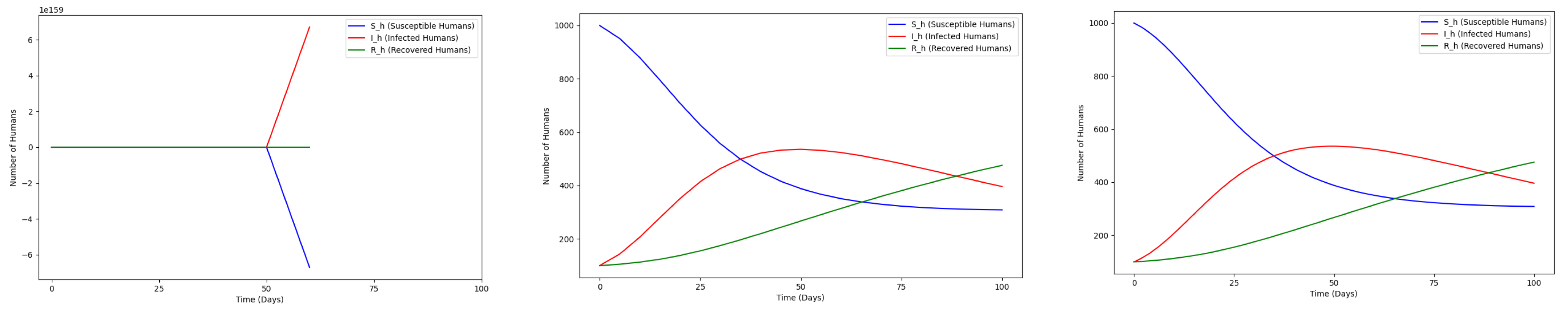
In Figure 2, we observe that the plots for the human components with RK4 for Δ t = 0.1 and Δ t = 5 are in agreement with the positivity and boundedness properties. However, for Δ t = 10 , the properties of the model are violated, resulting in non-physical behavior. This confirms that a restriction must be made on the step size for RK4 to converge.
Figure 3 proves that for Δ t = 10 , Δ t = 5 , and Δ t = 0.1 , the 1NSFD method preserves the positivity and boundedness of solutions for humans. This proves that the first-order NSFD method is stable, since it converges to a solution regardless of the step size.
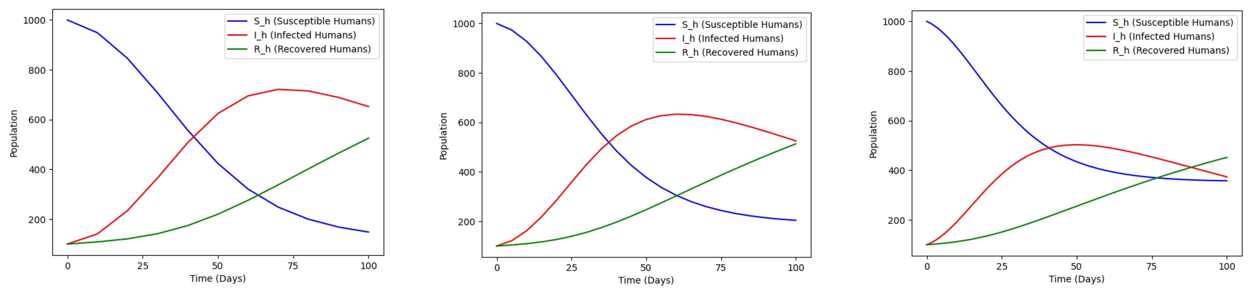
Figure 4 confirms Theorems 1 and 2, showing that the positivity and boundedness of solutions for the scheme (7) for humans are preserved for any given Δ t , since the numerical solutions for different step sizes remain within a biologically meaningful range and do not blow up as compared to Figure 2 when the step size is large. We observe the same in Figure 5, where different components of the mosquito population are plotted.
Table 2 shows the convergence of the RK4, 1NSFD, and 2NSFD methods to the solution for the different step sizes. One can perceive that for small step sizes, all schemes converge to the solution; on the other hand, as the step size increases, the RK4 method diverges away, while only the 1NSFD and 2NSFD methods converge to the solution regardless of the step size.
Since we do not have an exact solution of the continuous model (1), we use the double mesh principle to approximate how close the second-order NSFD (2NSFD) scheme (7) is to the true solution compared with the first-order NSFD (1NSFD) scheme (6). The error is approximated as
E D M = | S h ( Δ t ) ( t end ) S h ( Δ t 2 ) ( t end ) | + | I h ( Δ t ) ( t end ) I h ( Δ t 2 ) ( t end ) | + + | I v ( Δ t ) ( t end ) I v ( Δ t 2 ) ( t end ) | ,
and the convergence rate is approximated as
rate = log 2 E D M ( Δ t ) E D M ( Δ t / 2 ) .
Note 6.
In the formula (49), …represents the remaining error terms of  R h , A v , S v .
Using Equations (49) and (50), we have Table 3 and Table 4.
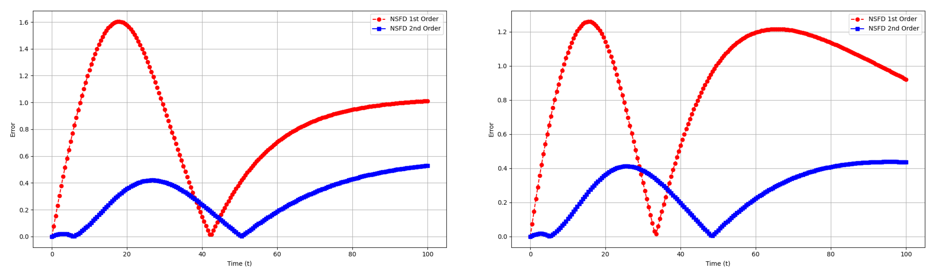
Both 2NSFD and 1NSFD are dynamically consistent with the continuous model, but Table 3 shows that 2NSFD is more accurate than 1NSFD. This analysis is further proved in Figure 6, where the error vectors estimated via the double mesh principle are plotted using 200 and 400 subintervals. The computational time for 2NSFD is more than that of 1NSFD, the reason being that the convergence of 2NSFD is facilitated by the denominator function, which needs to be updated at each iteration. This is in agreement with Remark 1, stating that the denominator function is calculated at every time step and for every population compartment.
Now we choose θ = 0 and two other different values to test their effects on errors.
Table 4 shows that as we increase values of θ , the error increases. A small error is obtained when we select the value of θ = 0 . All values of θ in Table 4 satisfy Corollary 20.
Remark 3.
It is worth noting that the value of the weight guarantees the stability of the underlying NSFD scheme. The weight must be a non-negative real number. In Table 4, the optimum weight is θ = 0 , which was derived from Corollary (20). This is simply a coincidence. In other situations, the optimum weight can be strictly positive (see, for example, [25]).

4. Conclusions

In this paper, we constructed the second-order NSFD method. The scheme preserves the key mathematical features of the continuous model, which are positivity, boundedness, equilibrium points, and stability. Numerical simulations confirm that the NSFD scheme (7) is indeed convergent of order two. Since we do not have an exact solution to the continuous model, we use the double mesh principle. From the numerical analysis, one can notice that for any value of weight ( θ ), the proposed nonstandard finite difference scheme converges to order two. However, a small error is obtained when θ = 0 , which satisfies the stability Theorem 3. Simulations validate Theorem 4, which states that the global error is very small. We also notice that the second-order NSFD scheme performs better in approximating the solution of malaria propagation, which can be applied to other infectious disease modeling. Moreover, the dynamics of malaria unfold over months to years. Standard numerical methods, such as Euler and Runge–Kutta methods, are not suitable for long time horizon dynamics because they would require small time steps, thus increasing computational complexity. The NSFD methodology has resolved the issue of time step restrictions. Therefore, the second-order NSFD scheme we proposed came as an improvement to the existing NSFD methods in terms of accuracy and stability. The present findings substantiate this by showing that as we increase the order of convergence, we minimize the errors and improve the accuracy of the approximation to the solution of highly nonlinear systems.

Author Contributions

Conceptualization: J.B.M.; formal analysis: J.B.M. and C.B.M.; investigation: C.B.M.; methodology: J.B.M. and C.B.M.; writing—original draft: C.B.M. All authors have read and agreed to the published version of the manuscript.

Funding

This research received no external funding.

Data Availability Statement

The original contributions presented in this study are included in the article. Further inquiries can be directed to the corresponding author(s).

Acknowledgments

The authors would like to appreciate meaningful criticism from unbiased reviewers that helped improve the quality of this paper.

Conflicts of Interest

The authors declare no conflicts of interest.

Abbreviations

The following abbreviations are used in this manuscript:
NSFDNonstandard finite difference
1NSFDFirst-order NSFD
2NSFDSecond-order NSFD

References

  1. Dimitrov, D.T.; Kojouharov, H.V. Nonstandard finite-difference schemes for general two-dimensional autonomous dynamical systems. Appl. Math. Lett. 2005, 18, 769–774. [Google Scholar] [CrossRef] [Scilit]
  2. Faragó, I.; Mosleh, R. Positively invariant semi-implicit discrete model for malaria propagation. Ann. Alexandru Ioan Cuza Univ. (New Ser.) Math. 2020, 2, 197–214. [Google Scholar]
  3. Lee, K.; Parish, E.J. Parameterized neural ordinary differential equations: Applications to computational physics problems. Proc. R. Soc. A 2021, 477, 20210162. [Google Scholar] [CrossRef] [Scilit]
  4. Ijaz, K.M.; Al-Khaled, K.; Raza, A.; Khan, S.U.; Omar, J.; Galal, A.M. Mathematical and numerical model for the malaria transmission: Euler method scheme for a malarial model. Int. J. Mod. Phys. B 2023, 37, 2350158. [Google Scholar] [CrossRef] [Scilit]
  5. Mosleh, R. Positivity Preserving Explicit Discrete Model for Malaria Propagation. Ann. Univ. Sci. Budapestinensis Rolando Eötvös Nomin. Sect. Math. 2020, 63, 123–133. [Google Scholar]
  6. Mickens, R.E. Discretizations of nonlinear differential equations using explicit nonstandard methods. J. Comput. Appl. Math. 1999, 110, 181–185. [Google Scholar] [CrossRef] [Scilit]
  7. Anguelov, R.; Dumont, Y.; Lubuma, J.M.S. On nonstandard finite difference schemes in biosciences. AIP Conf. Proc. 2012, 1487, 212–223. [Google Scholar] [CrossRef] [Scilit]
  8. Dimitrov, D.T.; Kojouharov, H.V. Positive and elementary stable nonstandard numerical methods with applications to predator-prey models. J. Comput. Appl. Math. 2006, 189, 98–108. [Google Scholar] [CrossRef] [Scilit]
  9. Gupta, M.; Slezak, J.M.; Alalhareth, F.; Roy, S.; Kojouharov, H.V. Second-order nonstandard explicit Euler method. AIP Conf. Proc. 2020, 2302, 110003. [Google Scholar] [CrossRef] [Scilit]
  10. Hoang, M.T. A class of second-order and dynamically consistent nonstandard finite difference schemes for nonlinear Volterra’s population growth model. Comput. Appl. Math. 2023, 42, 85. [Google Scholar] [CrossRef] [Scilit]
  11. Sarkar, T.; Srivastava, P.K.; Biswas, P. Application of the NSFD method in a Malaria model with nonlinear incidence and recovery rates. Eur. Phys. J. Plus 2024, 139, 275. [Google Scholar] [CrossRef] [Scilit]
  12. Hoang, M.T. A novel second-order nonstandard finite difference method for solving one-dimensional autonomous dynamical systems. Commun. Nonlinear Sci. Numer. Simul. 2022, 114, 106654. [Google Scholar] [CrossRef] [Scilit]
  13. Kojouharov, H.V.; Roy, S.; Gupta, M.; Alalhareth, F.; Slezak, J.M. A second-order modified nonstandard theta method for one-dimensional autonomous differential equations. Appl. Math. Lett. 2021, 112, 106775. [Google Scholar] [CrossRef] [Scilit]
  14. Hoang, M.T. High-order nonstandard finite difference methods preserving dynamical properties of one-dimensional dynamical systems. Numer. Algorithms 2025, 98, 219–249. [Google Scholar] [CrossRef] [Scilit]
  15. Qu, W.; Gu, Y.; Fan, C.M. A stable numerical framework for long-time dynamic crack. Int. J. Solids Struct. 2024, 293, 112768. [Google Scholar] [CrossRef] [Scilit]
  16. Hoang, M.T. A novel second-order nonstandard finite difference method preserving dynamical properties of a general single-species model. Int. J. Comput. Math. 2023, 100, 2047–2062. [Google Scholar] [CrossRef] [Scilit]
  17. Alalhareth, F.K.; Gupta, M.; Kojouharov, H.V.; Roy, S. Second-Order Modified Nonstandard Explicit Euler and Explicit Runge-Kutta Methods for n-Dimensional Autonomous Differential Equations. Computation 2024, 12, 183. [Google Scholar] [CrossRef] [Scilit]
  18. Oke, S.I.; Ojo, M.M.; Adeniyi, M.O.; Matadi, M.B. Mathematical modeling of malaria disease with control strategy. Commun. Math. Biol. Neurosci. 2020, 43, 1–29. [Google Scholar]
  19. Gurski, K.F. A simple construction of nonstandard finite-difference schemes for small nonlinear systems applied to SIR models. Comput. Math. Appl. 2013, 66, 2165–2177. [Google Scholar] [CrossRef] [Scilit]
  20. Wood, D.T.; Kojouharov, H.V. A class of nonstandard numerical methods for autonomous dynamical systems. Appl. Math. Lett. 2015, 50, 78–82. [Google Scholar] [CrossRef] [Scilit]
  21. Suryanto, A.; Darti, I. On the nonstandard numerical discretization of SIR epidemic model with a saturated incidence rate and vaccination. Am. Inst. Math. Sci. 2024, 6, 141–155. [Google Scholar] [CrossRef] [Scilit]
  22. Arenas, A.J.; González-Parra, G.; Chen-Charpentier, B.M. Construction of nonstandard finite difference schemes for the SI and SIR epidemic models of fractional order. J. Differ. Equ. Appl. 2008, 14, 1127–1147. [Google Scholar] [CrossRef] [Scilit]
  23. Hoang, M.T. Dynamical analysis of a generalized hepatitis B epidemic model and its dynamically consistent discrete model. Math. Comput. Simul. 2023, 205, 291–314. [Google Scholar] [CrossRef] [Scilit]
  24. Mickens, R.E. Nonstandard Finite Difference Models of Differential Equations; World Scientific: Singapore, 1994. [Google Scholar]
  25. Hoang, M.T.; Ehrhardt, M. A second-order nonstandard finite difference method for a general Rosenzweig-MacArthur predator-prey model. J. Comput. Appl. Math. 2024, 444, 115752. [Google Scholar] [CrossRef] [Scilit]
Figure 1. Flow diagram of malaria transmission between humans and mosquitoes.
Appliedmath 06 00036 g001
Figure 2. Runge–Kutta fourth-order (RK4) plots for humans with different step sizes. From left to right: Δ t = 10 , Δ t = 5 , and Δ t = 0.1 .
Appliedmath 06 00036 g002
Figure 3. First-order NSFD (1NSFD) plots for humans with different step sizes. From left to right: Δ t = 10 , Δ t = 5 , and Δ t = 0.1 .
Appliedmath 06 00036 g003
Figure 4. 2NSFD plots for humans with different step sizes. From left to right: Δ t = 10 , Δ t = 5 , and Δ t = 0.1 .
Appliedmath 06 00036 g004
Figure 5. 2NSFD plots for mosquitoes with different step sizes. From left to right: Δ t = 10 , Δ t = 5 , and Δ t = 0.1 .
Appliedmath 06 00036 g005
Figure 6. The errors versus time for 2NSFD and 1NSFD. ((Left): Susceptible humans; (Right): infected humans).
Appliedmath 06 00036 g006
Table 1. Values of parameters for numerical results.
ParameterDescriptionValue
π h Recruitment rate of humans 0.17
Ψ Per capita rate of loss of immunity in humans 0.0005275
μ h Natural mortality rate of humans 1 65 × 365
τ h Recovery rate of infectious individuals 0.0092
σ h Disease-induced death rate of humans 0.0003454
β h v Probability of effective transmission from humans to mosquitoes 0.24
β v h Probability of effective transmission from mosquitoes to humans 0.321
ϵ ( b ) Contact rate of mosquitoes with humans 0.271888
bProportion of treated net usage 0.53
π v Egg deposition rate of mosquitoes 1.84
γ v Maturation rate of immature mosquitoes 0.343
μ v Natural mortality rate of mosquitoes 1 18
Table 2. Numerical convergence of different methods to the solution for different step sizes.
Step SizeRK4 Method1NSFD Method2NSFD Method
0.1ConvergentConvergentConvergent
5ConvergentConvergentConvergent
10DivergentConvergentConvergent
20DivergentConvergentConvergent
100DivergentConvergentConvergent
Table 3. Difference between 2NSFD and 1NSFD methods in terms of errors, convergence rates, and computational time.
Δt2NSFD ErrorsRateTime(s)1NSFD ErrorsRateTime(s)
2 2 1.71 × 10 1 0.0084 1.12 × 10 1 0.000995
2 1 6.24 × 10 0 1.45340.0153 5.52 × 10 0 1.01680.000988
2 0 2.20 × 10 0 1.50160.0285 2.75 × 10 0 1.00490.002008
2 1 7.17 × 10 1 1.62070.0335 1.37 × 10 0 1.00190.006084
2 2 2.12 × 10 1 1.75830.0907 6.86 × 10 1 1.00080.013465
2 3 5.82 × 10 2 1.86260.0819 3.43 × 10 1 1.00030.022006
2 4 1.53 × 10 2 1.92660.2012 1.72 × 10 1 1.00010.038060
2 5 3.93 × 10 3 1.96200.3280 8.58 × 10 2 1.00010.069633
2 6 9.96 × 10 4 1.98070.5851 4.29 × 10 2 1.00000.133867
2 7 2.51 × 10 4 1.99031.0826 2.14 × 10 2 1.00000.263705
2 8 6.29 × 10 5 1.99512.1792 1.07 × 10 2 1.00000.505336
2 9 1.58 × 10 5 1.99754.8598 5.36 × 10 3 1.00001.021349
2 10 3.94 × 10 6 1.998810.4728 2.68 × 10 3 0.99962.021290
Table 4. Double mesh errors and convergence rate for 2NSFD.
ΔtError ( θ = 0 )RateError ( θ = 0.3 )RateError ( θ = 1 )Rate
2 2 1.71 × 10 1 2.05 × 10 1 2.26 × 10 1
2 1 6.24 × 10 0 1.45348.22 × 10 0 1.31759.88 × 10 0 1.1908
2 0 2.20 × 10 0 1.50163.07 × 10 0 1.42214.10 × 10 0 1.2678
2 1 7.17 × 10 1 1.62071.03 × 10 0 1.57301.53 × 10 0 1.4219
2 2 2.12 × 10 1 1.75833.13 × 10 1 1.72065.06 × 10 1 1.5979
2 3 5.82 × 10 2 1.86268.77 × 10 2 1.83451.50 × 10 1 1.7496
2 4 1.53 × 10 2 1.92662.34 × 10 2 1.90884.15 × 10 2 1.8569
2 5 3.93 × 10 3 1.96206.04 × 10 3 1.95191.10 × 10 2 1.9228
2 6 9.96 × 10 4 1.98071.54 × 10 3 1.97532.82 × 10 3 1.9598
2 7 2.51 × 10 4 1.99033.87 × 10 4 1.98757.14 × 10 4 1.9795
2 8 6.29 × 10 5 1.99519.73 × 10 5 1.99371.80 × 10 4 1.9896
2 9 1.58 × 10 5 1.99752.44 × 10 5 1.99684.51 × 10 5 1.9948
2 10 3.94 × 10 6 1.99886.10 × 10 6 1.99841.13 × 10 5 1.9974
Disclaimer/Publisher’s Note: The statements, opinions and data contained in all publications are solely those of the individual author(s) and contributor(s) and not of MDPI and/or the editor(s). MDPI and/or the editor(s) disclaim responsibility for any injury to people or property resulting from any ideas, methods, instructions or products referred to in the content.