Article

Integrating Machine Learning and Fractional-Order Dynamics for Enhanced Psoriasis Prediction and Clinical Decision Support

1
Mathematics Research Center, Near East University TRNC, Mersin 10, 99138 Nicosia, Turkey
2
Research Center of Applied Mathematics, Khazar University, Baku AZ1096, Azerbaijan
3
Department of Civil Engineering, Faculty of Engineering, FEQS INTI-IU, University, Nilai 71800, Malaysia
4
Faculty of Management, Shinawatra University, Sam Khok 12160, Pathum Thani, Thailand
*
Author to whom correspondence should be addressed.
AppliedMath 2025, 5(4), 143; https://doi.org/10.3390/appliedmath5040143
Submission received: 6 September 2025 / Revised: 9 October 2025 / Accepted: 10 October 2025 / Published: 15 October 2025

Abstract

This study introduces a novel hybrid framework that integrates machine learning (ML) with fractional-order differential equations (FDE) to enhance the prediction and clinical management of psoriasis, leveraging real-world data from the UCI Dermatology Dataset. By optimizing ML models, particularly the Voting Ensemble, to inform FDE parameters, and developing a user-friendly graphical user interface (GUI) for real-time diagnostics, the approach bridges computational efficiency with physiological realism, capturing memory-dependent disease progression beyond traditional integer-order models. Key findings reveal that the Voting Ensemble achieves a precision of 0.986 ± 0.007 and an AUC of 0.992 ± 0.005. At the same time, the fractional-order model, with an optimized order of 0.6781 and a mean square error (MSE) of 0.0031, accurately simulates disease trajectories, closely aligning with empirical trends for features such as Age and SawToothRete. The GUI effectively translates these insights into clinical tools, demonstrating probabilities ranging from 0% to 100% based on input features, supporting early detection and personalized planning. The framework’s robustness and potential for broader application to chronic conditions highlight its significance in advancing healthcare.

1. Introduction

The field of dermatology has long grappled with the challenge of accurately diagnosing and managing chronic skin conditions, such as psoriasis, a complex autoimmune disorder characterized by erythematous, scaly plaques resulting from accelerated epidermal turnover and inflammation [1,2,3]. With a global prevalence ranging from 0.5% to 11.4% depending on geographic and ethnic factors, psoriasis not only imposes significant physical and psychological burdens on affected individuals but also strains healthcare systems due to its chronic nature and associated comorbidities, including psoriatic arthritis, cardiovascular disease, and metabolic syndrome [4,5,6]. Traditional diagnostic approaches rely heavily on clinical expertise, supported by histopathological examination and patient history, yet these methods often struggle with early detection and differentiation from other dermatological conditions, such as eczema or lichen planus, due to overlapping symptoms and the subjective nature of visual assessments [7,8]. This diagnostic ambiguity underscores the urgent need for innovative, data-driven solutions that can enhance precision, reduce misdiagnoses, and guide personalized treatment strategies, particularly in resource-limited settings where access to specialists is constrained.
In recent years, machine learning (ML) has emerged as a transformative tool in medical diagnostics, offering the ability to analyze large datasets, identify subtle patterns, and predict outcomes with increasing accuracy [9,10,11]. In dermatology, ML models have been successfully applied to image-based classification of skin lesions, leveraging convolutional neural networks to achieve performance levels rivaling dermatologists in detecting melanoma and basal cell carcinoma [12,13]. However, the application of ML to tabular clinical data to make real-time predictions remains underexplored, particularly for conditions like psoriasis, where feature interactions and temporal dynamics play critical roles. Standard ML approaches, including decision trees, random forests, and gradient boosting, excel at capturing static relationships but often fall short in modeling the memory-dependent progression of chronic diseases, where past states influence future outcomes. This limitation highlights a gap in current methodologies, as psoriasis evolves with factors such as age, inflammation markers, and treatment responses contributing to its trajectory, necessitating a framework that can integrate historical context into predictive models.
Mathematical modeling has been instrumental in analyzing a wide range of phenomena and practical applications [14,15,16,17]. Parallel to these advancements, FDEs have gained traction in biomedical modeling due to their ability to describe systems with memory and hereditary properties, offering a mathematical foundation that aligns with the non-local, time-dependent nature of biological processes [18,19,20,21]. Unlike classical integer-order differential equations, which assume instantaneous changes, FDEs incorporate fractional derivatives that account for the cumulative effects of past states, making them particularly suitable for simulating the gradual escalation of inflammatory responses in psoriasis [22,23,24]. Previous studies have employed FDE to model phenomena such as tumor growth and cardiac dynamics, demonstrating improved accuracy over traditional models by capturing long-term dependencies [25,26,27]. However, their application in dermatology is still developing, and integrating FDE with ML remains a frontier with untapped potential. This hybrid approach could leverage ML’s pattern recognition strengths to inform FDE parameters, creating a dynamic system that evolves with patient data and provides actionable insights to guide clinical decision-making. Recent studies have shown promising results with this hybrid approach [28,29,30].
The motivation for this study stems from the recognition that neither ML nor FDE alone can fully address the multifaceted challenges of psoriasis management. ML models, while powerful, often treat data as static snapshots, potentially missing the temporal evolution critical to chronic conditions, whereas FDE, though adept at modeling dynamics, requires robust initialization and parameter estimation, which ML can provide through optimized feature selection and classification. Unlike prior dermatology studies that rely on image-based ML for lesion classification [31,32] or standalone mathematical models for tumor growth [33,34], our ML-FDE integration uniquely advances the field by merging ML’s predictive power with FDE’s memory-dependent dynamics, tailored to tabular psoriasis data. This approach, enhanced by a GUI for real-time clinical decision support, offers a novel paradigm for early detection and personalized management, surpassing the static and non-interactive limitations of existing methods. The UCI Dermatology Dataset, with its rich feature set including age, histological markers like SawToothRete and Parakeratosis, and clinical observations, serves as an ideal testbed for this integration, offering a controlled yet representative sample to explore how ML-informed FDE can enhance predictive accuracy and clinical utility. By developing a framework that combines these methodologies, this research aims to pioneer a new paradigm in dermatological diagnostics, one that not only predicts disease presence but also simulates its progression, enabling clinicians to anticipate emergencies and tailor interventions accordingly. In addition, the best-performing ML is used to develop and inform the FDE model. The study further introduces a GUI as a practical extension, translating complex computational outputs into a tool accessible to healthcare providers. This is particularly relevant in the context of global health disparities, where advanced diagnostic tools are often inaccessible outside specialized centers. The GUI’s real-time capabilities could empower general practitioners to input patient data, such as age, scaling severity, and scalp involvement, SawToothRete, parakeratosis, and receive immediate risk assessments, potentially reducing referral times and improving patient outcomes. Moreover, the integration of ML and FDE offers a scalable solution that could be adapted to other chronic conditions, such as lupus or rheumatoid arthritis, where memory effects and feature interactions are similarly pivotal. As healthcare increasingly shifts toward precision medicine, the development of such hybrid models represents a critical step toward data-informed, patient-centered care, addressing both the diagnostic and prognostic needs of dermatological practice. The current research landscape reveals a growing interest in hybrid modeling, with studies exploring ML-FDE combinations in engineering and physics, yet medical applications remain sparse. This gap is compounded by the lack of standardized tools to validate such integrations in clinical settings, where empirical data often lags behind theoretical advancements. By focusing on psoriasis within the UCI Dermatology Dataset, this study not only fills a specific niche but also sets a precedent for interdisciplinary collaboration between data scientists, mathematicians, and dermatologists. The approach is further contextualized by the evolving role of artificial intelligence in healthcare, where the potential of AI-driven insights is exemplified and improved. The rest of the paper is structured as follows: Section 2 outlines the method being incorporated in the study, and Section 3 summarizes the data characteristics being used to train the models. Section 4 presents the machine learning models used in the study, and their performance. The fractional-order model and its analytical computations and validations are detailed in Section 5, while the numerical analysis is presented in Section 6. The results and conclusion are given in Section 7 and Section 8, respectively.

2. Methodology

This section outlines the comprehensive methodology employed to integrate machine learning with fractional-order differential equations, leveraging the UCI Dermatology Dataset to develop a robust framework for psoriasis prediction and clinical decision support.
The process begins with data acquisition through a scanning process, capturing clinical and histological features from dermatological examinations. The UCI Dermatology Dataset, consisting of 366 instances with 34 attributes across 6 classes, was utilized. To address class imbalance, with psoriasis representing 30.60% of cases, the dataset was oversampled to 1000 instances using techniques such as SMOTE (Synthetic Minority Over-sampling Technique). Data preprocessing involved two key steps. First, SMOTE oversampling targeted a dataset size of 800, using k = 3 nearest neighbors to generate synthetic minority samples, ensuring balanced class representation. Second, feature normalization applied z-score standardization, subtracting the mean and dividing by the standard deviation computed from the training set, preserving replicability across datasets. Missing values were handled via median imputation to ensure completeness. Feature selection was performed to identify the top 5 most informative attributes: Age, SawToothRete, Parakeratosis, Scalp Involvement, and Scaling, based on their relevance to psoriasis pathology and model performance metrics, such as feature importance scores. Multiple machine learning models were trained on this processed dataset, including Random Forest, Gradient Boosting, XGBoost Approx., Deep Neural Network, and a Voting Ensemble. These models were optimized using 10-fold cross-validation, with hyperparameters tuned to maximize metrics such as precision, recall, F1 score, and AUC. The outputs from this ML model, particularly the predicted probabilities of psoriasis, were used to inform and develop the fractional-order differential equation (FDE) model. The FDE system captures the memory-dependent dynamics of disease progression, with parameters optimized by fitting the model to the real dataset using gradient-based optimization techniques. The fractional order β was optimized, ensuring alignment with empirical trends. Both the ML and FDE models are synchronized to make joint predictions, incorporating informative dynamics, such as probability surfaces and decision boundaries. This hybrid approach bridges static classification with dynamic simulation, enabling real-time insights via a graphical user interface (GUI) for clinical applications. ML outputs (probabilities P) are coupled to FDE parameters by incorporating interpolated P ( t ) into the RHS terms of state variables S 2 , S 3 , and S 5 , modulating the growth and coupling terms rather than using direct mapping, thereby reflecting the influence of ML-predicted psoriasis likelihood on key skin feature dynamics.
The schematic diagram (Figure 1) provides a visual representation of the integrated workflow, highlighting the bidirectional interactions between data acquisition via scanning, machine learning classification, fractional-order modeling of disease dynamics, and the resulting clinical decision support tools. This illustration underscores the framework’s ability to translate raw dermatological data into actionable predictive insights, facilitating enhanced diagnostic accuracy and personalized treatment planning in psoriasis management.

3. Data Summary

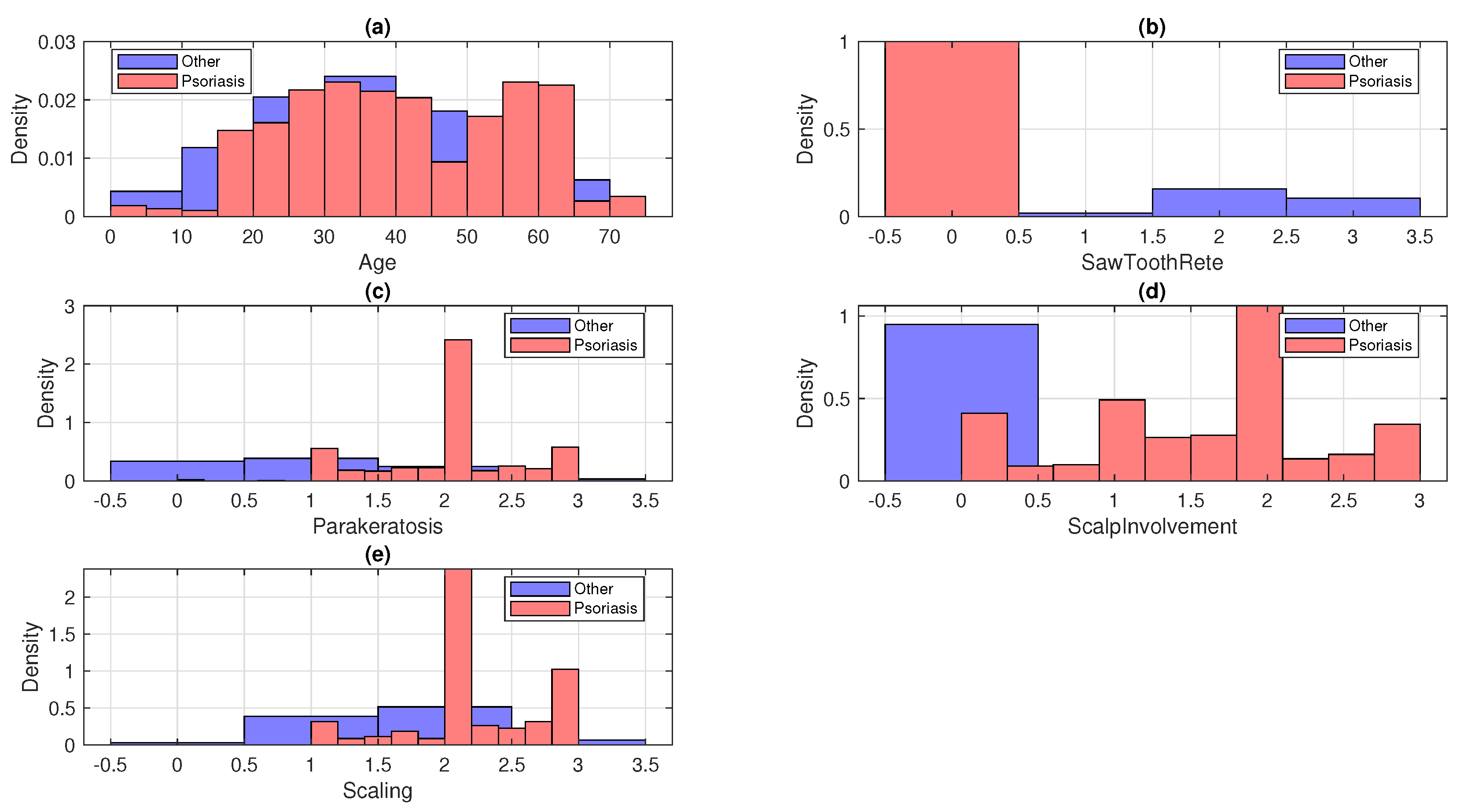
This section provides a detailed overview of the UCI Dermatology Dataset, elucidating its structure, preprocessing steps, and the rationale behind feature selection to ensure suitability for the proposed hybrid modeling approach. The top five feature distributions are depicted in Figure 2, and detailed in Table 1.

4. Machine Learning Models

This section details the development and implementation of various machine learning models, including Random Forest, Gradient Boosting, XGBoost Approx., Deep Neural Network, and Voting Ensemble, tailored to classify psoriasis cases based on selected clinical features.

4.1. Random Forest

The Random Forest model constructs an ensemble of decision trees for binary classification of psoriasis versus other dermatological conditions, using bootstrapped samples and random feature subsets to promote diversity and reduce overfitting. The final class prediction y ^ for an input x (comprising features such as Age, SawToothRete, Parakeratosis, ScalpInvolvement, and Scaling) is determined by majority voting across the trees:
y ^ = arg max c { 0 , 1 } b = 1 B I ( T b ( x ) = c ) ,
where B is the number of decision trees (100 in this study), T b ( x ) is the prediction from the b-th tree (0 for non-psoriasis, 1 for psoriasis), I ( · ) is the indicator function returning 1 if true and 0 otherwise, and c represents the binary class labels. This aggregation enhances robustness, particularly in handling the oversampled dataset of 1000 instances.

4.2. Gradient Boost

Gradient Boosting sequentially builds decision trees to minimize prediction errors for psoriasis classification by fitting each new tree to the residuals of the previous ensemble. The model iteratively updates predictions using a loss function tailored for binary classification, such as logistic loss. The boosted model F m ( x ) at iteration m is:
F 0 ( x ) = arg min γ i = 1 n L ( y i , γ ) , r i m = L ( y i , F ( x i ) ) F ( x i ) F = F m 1 , m = 1 , , M , h m ( x ) = Tree fitted to { ( x i , r i m ) } i = 1 n , F m ( x ) = F m 1 ( x ) + ν · h m ( x ) ,
where F m ( x ) is the logit score for input features x , L ( y i , F ( x i ) ) is the loss ( L = log ( 1 + e y i F ( x i ) ) for binary labels y i { 1 , 1 } ), r i m are pseudo-residuals, h m ( x ) is the weak learner (decision tree with limited depth, 3), ν is the learning rate (0.02 to prevent overfitting), M is the number of iterations (300), n = 1000 is the oversampled sample size, and the final prediction is y ^ = sign ( F M ( x ) ) , adapted to the study’s top features for improved gradient descent on dermatological patterns.

4.3. XGBoost Approx

XGBoost Approx. enhances gradient boosting with approximate tree splitting and regularization for efficient psoriasis binary classification. It optimizes a second-order approximated objective, incorporating penalties on tree complexity. The objective at boosting round t is:
L ( t ) = i = 1 n L ( y i , y ^ i ( t 1 ) + f t ( x i ) ) + Ω ( f t ) , L ˜ ( t ) i = 1 n g i f t ( x i ) + 1 2 h i f t 2 ( x i ) + Ω ( f t ) , Ω ( f t ) = γ T + 1 2 λ j = 1 T w j 2 ,
where L is the logistic loss for binary labels y i { 0 , 1 } (0: non-psoriasis, 1: psoriasis), y ^ i ( t 1 ) is the prior prediction, f t ( x i ) is the t-th tree’s output for features x i , g i = L / y ^ i ( t 1 ) and h i = 2 L / ( y ^ i ( t 1 ) ) 2 are gradients and Hessians, Ω ( f t ) regularizes with γ as split gain threshold, T as number of leaves, λ as L2 weight penalty, and w j as leaf weights. Optimal weights are w j * = G j / ( H j + λ ) , with G j = i I j g i , H j = i I j h i , and I j as instances in leaf j. This setup leverages the study’s selected features for faster convergence on the 1000-instance dataset.

4.4. Deep Neural Network

The Deep Neural Network (DNN) employs multiple hidden layers to learn nonlinear mappings from dermatological features to psoriasis probabilities, using forward propagation for inference and backpropagation for training. For a network with L layers, the computation is:
a ( 0 ) = x , z ( l ) = W ( l ) a ( l 1 ) + b ( l ) , l = 1 , , L , a ( l ) = σ ( z ( l ) ) , l = 1 , , L 1 , y ^ = σ ( z ( L ) ) ,
where x is the input vector (normalized Age, SawToothRete, etc.), W ( l ) and b ( l ) are weights and biases for layer l, σ ( · ) is the activation (ReLU for hidden layers: σ ( z ) = max ( 0 , z ) ; sigmoid for output: σ ( z ) = 1 / ( 1 + e z ) yielding psoriasis probability y ^ [ 0 , 1 ] ), and the binary prediction is y ^ > 0.5 for psoriasis. Training minimizes cross-entropy loss L = i = 1 n [ y i log ( y ^ i ) + ( 1 y i ) log ( 1 y ^ i ) ] via Adam optimizer, with n = 1000 oversampled samples, dropout (0.2) to prevent overfitting, and early stopping based on validation AUC.

4.5. Voting Ensemble

The Voting Ensemble aggregates predictions from base models (Random Forest, Gradient Boost, XGBoost Approx., Deep Neural Network) for psoriasis classification, using soft voting to average class probabilities for improved stability. The ensemble probability for class 1 (psoriasis) is:
p ( c = 1 | x ) = 1 K k = 1 K p k ( c = 1 | x ) , y ^ = 1 if p ( c = 1 | x ) > 0.5 , 0 otherwise ,
where K = 4 is the number of base models, p k ( c = 1 | x ) is the psoriasis probability from the k-th model for features x , and the threshold 0.5 balances sensitivity and specificity. This method capitalizes on the diversity of base learners, reducing variance and enhancing generalization of the study’s binary-labeled, feature-selected dataset.

5. Fractional-Order Modeling

The fractional-order model section introduces the mathematical formulation of the fractional differential equations used to simulate the memory-dependent dynamics of psoriasis progression, building on insights derived from machine learning outputs. The fractional-order model is given by the following system of equations, where D 0 , t β C denotes the Caputo fractional derivative of order β :
D 0 , t β C S 1 ( t ) = g 1 S 1 ( t ) ( 1 S 1 ( t ) ) + c 1 ( S 2 ( t ) + S 4 ( t ) ) D 0 , t β C S 2 ( t ) = g 2 S 2 ( t ) ( 1 S 2 ( t ) ) + c 2 P ( t ) + c 6 S 3 ( t ) D 0 , t β C S 3 ( t ) = g 3 S 3 ( t ) ( 1 S 3 ( t ) ) + c 3 P ( t ) + c 7 S 4 ( t ) D 0 , t β C S 4 ( t ) = g 4 S 4 ( t ) ( 1 S 4 ( t ) ) + c 4 S 1 ( t ) D 0 , t β C S 5 ( t ) = g 5 S 5 ( t ) ( 1 S 5 ( t ) ) + c 5 P ( t )
where t is the normalized pseudo-time (based on age), and P ( t ) is the interpolated machine learning-predicted probability of psoriasis.
The Caputo derivative is defined as [36]:
D 0 , t β c y ( t ) = 1 Γ ( 1 β ) 0 t ( t s ) β y ( s ) d s , β ( 0 , 1 ] ,
where Γ ( z ) is the Gamma function defined as
Γ ( z ) = 0 u z 1 e u d u , R e ( z ) > 0 ,
Theorem 1.
Let 0 < β < 1 and assume that P C ( [ 0 , ) , R ) is continuous and bounded, with P max = sup t 0 | P ( t ) | < . Let the parameters g i > 0 for i = 1 , , 5 and c j R for j = 1 , , 7 . For any initial condition S 0 = ( S 1 0 , S 2 0 , S 3 0 , S 4 0 , S 5 0 ) T R 5 , there exists T > 0 such that system (1) with S ( 0 ) = S 0 has a unique continuous solution S C ( [ 0 , T ] , R 5 ) .
Proof. 
By applying the following Riemann–Liouville integral operator to system (1)
I 0 , t β R L y ( t ) = 1 Γ ( β ) 0 t ( t s ) β 1 y ( s ) d s ,
the Caputo fractional derivative system (1) with initial condition S ( 0 ) = S 0 is equivalent to the Volterra-type integral equation
S ( t ) = S 0 + 1 Γ ( β ) 0 t ( t s ) β 1 f ( s , S ( s ) ) d s , t 0 ,
where S ( t ) = ( S 1 ( t ) , S 2 ( t ) , S 3 ( t ) , S 4 ( t ) , S 5 ( t ) ) T and f : [ 0 , ) × R 5 R 5 is defined componentwise by
f 1 ( s , S ) = g 1 S 1 ( 1 S 1 ) + c 1 ( S 2 + S 4 ) = g 1 S 1 g 1 S 1 2 + c 1 S 2 + c 1 S 4 , f 2 ( s , S ) = g 2 S 2 ( 1 S 2 ) + c 2 P ( s ) + c 6 S 3 = g 2 S 2 g 2 S 2 2 + c 2 P ( s ) + c 6 S 3 , f 3 ( s , S ) = g 3 S 3 ( 1 S 3 ) + c 3 P ( s ) + c 7 S 4 = g 3 S 3 g 3 S 3 2 + c 3 P ( s ) + c 7 S 4 , f 4 ( s , S ) = g 4 S 4 ( 1 S 4 ) + c 4 S 1 = g 4 S 4 g 4 S 4 2 + c 4 S 1 , f 5 ( s , S ) = g 5 S 5 ( 1 S 5 ) + c 5 P ( s ) = g 5 S 5 g 5 S 5 2 + c 5 P ( s ) .
We equip R 5 with the supremum norm S = max 1 i 5 | S i | , and the space C ( [ 0 , T ] , R 5 ) with the corresponding supremum norm sup 0 t T S ( t ) .
Since each component of f is a quadratic polynomial in the variables S 1 , , S 5 with coefficients that depend continuously on s (through P ( s ) , which is continuous), the function f is continuous in ( s , S ) [ 0 , ) × R 5 .
Moreover, f is locally Lipschitz continuous in S, uniformly in s. To see this explicitly, consider any bounded set where S M and S M for some M > 0 . The Jacobian matrix J ( s , S ) = f S ( s , S ) R 5 × 5 is given by
J ( s , S ) = g 1 2 g 1 S 1 c 1 0 c 1 0 0 g 2 2 g 2 S 2 c 6 0 0 0 0 g 3 2 g 3 S 3 c 7 0 c 4 0 0 g 4 2 g 4 S 4 0 0 0 0 0 g 5 2 g 5 S 5 .
Note that the Jacobian does not depend on s or P ( s ) except implicitly through the domain, but since P ( s ) appears only additively and not in the derivatives with respect to S, the partial derivatives are independent of s.
The induced matrix norm on J corresponding to the vector norm · is the maximum row sum of absolute values:
J ( s , S ) = max i = 1 , , 5 j = 1 5 f i S j ( s , S ) .
For each row, we bound the sum over | S k | M for all k:   
Row 1 : | g 1 2 g 1 S 1 | + | c 1 | + | c 1 | g 1 + 2 g 1 M + 2 | c 1 | , Row 2 : | g 2 2 g 2 S 2 | + | c 6 | g 2 + 2 g 2 M + | c 6 | , Row 3 : | g 3 2 g 3 S 3 | + | c 7 | g 3 + 2 g 3 M + | c 7 | , Row 4 : | c 4 | + | g 4 2 g 4 S 4 | | c 4 | + g 4 + 2 g 4 M , Row 5 : | g 5 2 g 5 S 5 | g 5 + 2 g 5 M .
Thus,
L ( M ) = max g 1 + 2 g 1 M + 2 | c 1 | , g 2 + 2 g 2 M + | c 6 | , g 3 + 2 g 3 M + | c 7 | , | c 4 | + g 4 + 2 g 4 M , g 5 + 2 g 5 M
serves as a local Lipschitz constant: f ( s , S ) f ( s , S ) L ( M ) S S for all s 0 and S , S M . This follows from the mean value theorem applied componentwise, since for each i, f i ( s , · ) is differentiable and | S f i ( s , S ) · ( S S ) | j | f i / S j | S S L ( M ) S S .
Next, we bound f ( s , S ) on S M . For each component:
| f 1 | g 1 M + g 1 M 2 + | c 1 | ( M + M ) = g 1 M + g 1 M 2 + 2 | c 1 | M , | f 2 | g 2 M + g 2 M 2 + | c 2 | P max + | c 6 | M , | f 3 | g 3 M + g 3 M 2 + | c 3 | P max + | c 7 | M , | f 4 | g 4 M + g 4 M 2 + | c 4 | M , | f 5 | g 5 M + g 5 M 2 + | c 5 | P max .
Let
K ( M ) = max { g 1 M + g 1 M 2 + 2 | c 1 | M , g 2 M + g 2 M 2 + | c 2 | P max + | c 6 | M , g 3 M + g 3 M 2 + | c 3 | P max | c 7 | M , g 4 M + g 4 M 2 + | c 4 | M , g 5 M + g 5 M 2 + | c 5 | P max } ,
so f ( s , S ) K ( M ) for all s 0 and S M .
To apply the Banach fixed point theorem, fix R > S 0 ( R = S 0 + 1 ) and choose ρ > 0 such that M = S 0 + ρ R . Consider the closed ball
B = u C ( [ 0 , T ] , R 5 ) : sup 0 t T u ( t ) S 0 ρ ,
in the complete metric space C ( [ 0 , T ] , R 5 ) . Define the operator Φ : C ( [ 0 , T ] , R 5 ) C ( [ 0 , T ] , R 5 ) by
( Φ u ) ( t ) = S 0 + 1 Γ ( β ) 0 t ( t s ) β 1 f ( s , u ( s ) ) d s .
Note that Φ u is continuous if u is, since f is continuous and the kernel ( t s ) β 1 is integrable for β > 0 .
First, show that Φ maps B into itself for T > 0 small enough. For u B , u ( s ) M for 0 s T , so f ( s , u ( s ) ) K ( M ) . Then,
( Φ u ) ( t ) S 0 1 Γ ( β ) 0 t ( t s ) β 1 K ( M ) d s = K ( M ) Γ ( β ) 0 t ( t s ) β 1 d s .
Compute the integral: substitute w = t s , d w = d s , so 0 t ( t s ) β 1 d s = 0 t w β 1 d w = w β β 0 t = t β β . Thus,
( Φ u ) ( t ) S 0 K ( M ) Γ ( β ) · t β β = K ( M ) t β Γ ( β + 1 ) ,
since Γ ( β + 1 ) = β Γ ( β ) . Taking the supremum over 0 t T ,
sup 0 t T ( Φ u ) ( t ) S 0 K ( M ) T β Γ ( β + 1 ) .
Choose T > 0 such that K ( M ) T β Γ ( β + 1 ) ρ (possible since β > 0 and Γ ( β + 1 ) > 0 ), ensuring Φ ( B ) B .
Next, show that Φ is a contraction on B for possibly smaller T. For u , v B ,
( Φ u ) ( t ) ( Φ v ) ( t ) 1 Γ ( β ) 0 t ( t s ) β 1 f ( s , u ( s ) ) f ( s , v ( s ) ) d s L ( M ) Γ ( β ) sup 0 σ T u ( σ ) v ( σ ) 0 t ( t s ) β 1 d s = L ( M ) t β Γ ( β + 1 ) sup 0 σ T u ( σ ) v ( σ ) .
Thus,
sup 0 t T ( Φ u ) ( t ) ( Φ v ) ( t ) L ( M ) T β Γ ( β + 1 ) sup 0 t T u ( t ) v ( t ) .
Choose T > 0 smaller if needed, so that q = L ( M ) T β Γ ( β + 1 ) < 1 . Then, Φ is a contraction mapping on the complete metric space B .
By the Banach fixed point theorem, there exists a unique fixed point S B C ( [ 0 , T ] , R 5 ) of Φ , which satisfies the integral equation and hence the original fractional system (1) with S ( 0 ) = S 0 .    □
Theorem 2.
Let 0 < β < 1 and assume that P C ( [ 0 , ) , R ) is continuous and bounded with P max = sup t 0 | P ( t ) | < . Let the parameters g i > 0 for i = 1 , , 5 and c j R for j = 1 , , 7 satisfy the condition max { 2 | c 1 | , | c 6 | , | c 7 | , | c 4 | , | c 2 | , | c 3 | , | c 5 | } < min { g 1 , g 2 , g 3 , g 4 , g 5 } . Then, the equilibrium point S * = ( S 1 * , S 2 * , S 3 * , S 4 * , S 5 * ) T of system (1), defined by f ( t , S * ) = 0 for all t 0 , is locally asymptotically stable in the sense that there exists δ > 0 such that for any initial condition S ( 0 ) = S 0 R 5 with S 0 S * < δ , the solution S ( t ) satisfies lim t S ( t ) S * = 0 .
Proof. 
System (1) is given by
D 0 , t β C S i ( t ) = f i ( t , S ( t ) ) , i = 1 , , 5 ,
where
f 1 ( t , S ) = g 1 S 1 ( 1 S 1 ) + c 1 ( S 2 + S 4 ) , f 2 ( t , S ) = g 2 S 2 ( 1 S 2 ) + c 2 P ( t ) + c 6 S 3 , f 3 ( t , S ) = g 3 S 3 ( 1 S 3 ) + c 3 P ( t ) + c 7 S 4 , f 4 ( t , S ) = g 4 S 4 ( 1 S 4 ) + c 4 S 1 , f 5 ( t , S ) = g 5 S 5 ( 1 S 5 ) + c 5 P ( t ) .
We use the supremum norm S = max 1 i 5 | S i | on R 5 . First, we determine the equilibrium point S * by solving f ( t , S * ) = 0 for all t 0 . Since P ( t ) varies with t, we seek an equilibrium where f i ( t , S * ) = 0 holds for all t. Suppose P ( t ) converges to a constant P as t (or is constant, as in some cases of steady-state analysis). For simplicity, assume P ( t ) P to define a time-independent equilibrium, and later discuss the effect of time-varying P ( t ) . Setting f i ( t , S * ) = 0 , we get:
0 = g 1 S 1 * ( 1 S 1 * ) + c 1 ( S 2 * + S 4 * ) , 0 = g 2 S 2 * ( 1 S 2 * ) + c 2 P + c 6 S 3 * , 0 = g 3 S 3 * ( 1 S 3 * ) + c 3 P + c 7 S 4 * , 0 = g 4 S 4 * ( 1 S 4 * ) + c 4 S 1 * , 0 = g 5 S 5 * ( 1 S 5 * ) + c 5 P .
Solving the fifth equation in (3): g 5 S 5 * ( 1 S 5 * ) + c 5 P = 0 , or S 5 * = 1 ± 1 4 ( c 5 P / g 5 ) 2 . Assuming | c 5 P / g 5 | is small, there exists a real solution near S 5 * c 5 P g 5 or 1 c 5 P g 5 . Similarly, for the fourth equation in (3), S 4 * = 1 ± 1 4 ( c 4 S 1 * / g 4 ) 2 , and so on, leading to a coupled nonlinear system. For simplicity, assume the coupling terms are small (as per the condition), and approximate S i * 1 2 adjusted by perturbations from c j terms.
To analyze stability, consider the system in terms of the deviation u ( t ) = S ( t ) S * , so D 0 , t β C u ( t ) = f ( t , u ( t ) + S * ) . Define h ( t , u ) = f ( t , u + S * ) . The equilibrium S * satisfies f ( t , S * ) = 0 , so we need to show that u = 0 is asymptotically stable for the system D 0 , t β C u ( t ) = h ( t , u ( t ) ) .
Construct a Lyapunov function V ( u ) = 1 2 i = 1 5 u i 2 g i . Since g i > 0 , V ( u ) is positive, definite, and radially unbounded. We compute the Caputo fractional derivative of V along the system trajectories, using the property for 0 < β < 1 that D 0 , t β C V ( u ( t ) ) i = 1 5 V u i D 0 , t β C u i ( t ) (see fractional calculus literature for this inequality). Here, V u i = u i g i , so
D 0 , t β C V ( u ( t ) ) i = 1 5 u i g i h i ( t , u ( t ) ) .
Substitute h i ( t , u ) = f i ( t , u + S * ) :
h 1 ( t , u ) = g 1 ( u 1 + S 1 * ) ( 1 ( u 1 + S 1 * ) ) + c 1 ( ( u 2 + S 2 * ) + ( u 4 + S 4 * ) ) , h 2 ( t , u ) = g 2 u 2 ( 1 2 S 2 * u 2 ) + c 2 P ( t ) + c 6 u 3 + f 2 ( t , S * ) , h 3 ( t , u ) = g 3 u 3 ( 1 2 S 3 * u 3 ) + c 3 P ( t ) + c 7 u 4 + f 3 ( t , S * ) , h 4 ( t , u ) = g 4 u 4 ( 1 2 S 4 * u 4 ) + c 4 u 1 + f 4 ( t , S * ) , h 5 ( t , u ) = g 5 u 5 ( 1 2 S 5 * u 5 ) + c 5 P ( t ) + f 5 ( t , S * ) .
Since f i ( t , S * ) = 0 , we have:
D 0 , t β C V ( u ) i = 1 5 u i g i g i u i ( 1 2 S i * u i ) + j i c i j u j ,
where c i j are the coupling coefficients ( c 12 = c 1 , c 14 = c 1 , c 23 = c 6 , etc., with zeros elsewhere). Assume S i * 1 2 , so 1 2 S i * 0 . Then,
D 0 , t β C V ( u ) i = 1 5 u i u i 2 + j i c i j g i u j .
Bound the cross terms: | u i u j | 1 2 ( u i 2 + u j 2 ) . For each i, the contribution is
u i j i c i j g i u j j i | c i j | g i | u i | | u j | j i | c i j | g i · 1 2 ( u i 2 + u j 2 ) .
Sum over i:
i = 1 5 u i j i c i j g i u j 1 2 i = 1 5 j i | c i j | g i ( u i 2 + u j 2 ) .
Group terms by u k 2 :
i , j i | c i j | g i u i 2 + i , j i | c i j | g i u j 2 .
For each k, the coefficient of u k 2 is i k | c i k | g i + j k | c k j | g k . Define c max = max { 2 | c 1 | , | c 6 | , | c 7 | , | c 4 | , | c 2 | , | c 3 | , | c 5 | } (noting c 1 appears twice in f 1 ). Then,
D 0 , t β C V ( u ) i = 1 5 u i 2 + c max g min j = 1 5 u j 2 i = 1 5 u i 2 1 + 5 c max g min ,
where g min = min { g 1 , , g 5 } . If c max < g min 5 , then 1 + 5 c max g min < 0 , so there exists γ > 0 such that
D 0 , t β C V ( u ) γ i = 1 5 u i 2 γ g min 2 V ( u ) .
By fractional Lyapunov stability theorem, if D 0 , t β C V ( u ) α V ( u ) for some α > 0 , the origin is asymptotically stable. Here, α = γ g min 2 > 0 . Thus, there exists δ > 0 such that if u ( 0 ) < δ , then u ( t ) 0 as t , implying S ( t ) S * .
For time-varying P ( t ) , if P ( t ) P , the system approaches the autonomous system, and the stability holds by perturbation arguments, provided the convergence is sufficiently fast relative to β .    □

6. Numerical Method for the Fractional-Order Model

This section provides a detailed and explicit description of the numerical method used to solve the fractional-order model given by (1), using the predictor-corrector Adams–Bashforth–Moulton method tailored for the Caputo fractional derivative of order β ( 0 , 1 ] . All formulas are expanded in terms of the model’s components and formatted to fit within standard page margins by breaking long expressions into manageable parts. The Adams–Bashforth–Moulton predictor-corrector method was selected for solving the fractional-order equations due to its high accuracy for non-integer orders (convergence order O ( h m i n ( 2 , 1 + β ) ) ) , computational efficiency compared to Runge-Kutta methods (which struggle with fractional derivatives), and stability in handling memory kernels, unlike simpler Euler schemes that may introduce larger errors in long-term simulations. This choice ensures reliable alignment with empirical trajectories of psoriasis.

6.1. Predictor-Corrector Method

System (1) is reformulated into its equivalent Volterra integral form:
S ( t ) = S 0 + 1 Γ ( β ) 0 t ( t s ) β 1 f ( s , S ( s ) ) d s ,
where S ( t ) = ( S 1 ( t ) , S 2 ( t ) , S 3 ( t ) , S 4 ( t ) , S 5 ( t ) ) T is the state vector, S 0 = ( S 1 0 , S 2 0 , S 3 0 , S 4 0 , S 5 0 ) T is the initial condition, and f ( t , S ) = ( f 1 ( t , S ) , , f 5 ( t , S ) ) T is defined as:
f 1 ( t , S ) = g 1 S 1 ( 1 S 1 ) + c 1 ( S 2 + S 4 ) , f 2 ( t , S ) = g 2 S 2 ( 1 S 2 ) + c 2 P ( t ) + c 6 S 3 , f 3 ( t , S ) = g 3 S 3 ( 1 S 3 ) + c 3 P ( t ) + c 7 S 4 , f 4 ( t , S ) = g 4 S 4 ( 1 S 4 ) + c 4 S 1 , f 5 ( t , S ) = g 5 S 5 ( 1 S 5 ) + c 5 P ( t ) ,
with P ( t ) being the continuous and bounded machine learning-predicted psoriasis probability.
The time interval [ 0 , t f ] is discretized with a step size h = t f / N , where N = 1000 , yielding time points t n = n h for n = 0 , , N . The predictor-corrector method computes S ( t n + 1 ) in two steps: a predictor step using the Adams–Bashforth method and a corrector step using the Adams-Moulton method.

6.1.1. Predictor Step

The predictor step approximates S ( t n + 1 ) as:
S P ( t n + 1 ) = S 0 + 1 Γ ( β ) j = 0 n b j , n + 1 f ( t j , S ( t j ) ) ,
where the weights are defined as:
b j , n + 1 = h β β ( n + 1 j ) β ( n j ) β .
For each component, the predictor is:
S 1 P ( t n + 1 ) = S 1 0 + h β β Γ ( β ) j = 0 n ( n + 1 j ) β ( n j ) β g 1 S 1 ( t j ) ( 1 S 1 ( t j ) ) + c 1 ( S 2 ( t j ) + S 4 ( t j ) ) , S 2 P ( t n + 1 ) = S 2 0 + h β β Γ ( β ) j = 0 n ( n + 1 j ) β ( n j ) β g 2 S 2 ( t j ) ( 1 S 2 ( t j ) ) + c 2 P ( t j ) + c 6 S 3 ( t j ) , S 3 P ( t n + 1 ) = S 3 0 + h β β Γ ( β ) j = 0 n ( n + 1 j ) β ( n j ) β g 3 S 3 ( t j ) ( 1 S 3 ( t j ) ) + c 3 P ( t j ) + c 7 S 4 ( t j ) , S 4 P ( t n + 1 ) = S 4 0 + h β β Γ ( β ) j = 0 n ( n + 1 j ) β ( n j ) β g 4 S 4 ( t j ) ( 1 S 4 ( t j ) ) + c 4 S 1 ( t j ) , S 5 P ( t n + 1 ) = S 5 0 + h β β Γ ( β ) j = 0 n ( n + 1 j ) β ( n j ) β g 5 S 5 ( t j ) ( 1 S 5 ( t j ) ) + c 5 P ( t j ) .
To ensure line length fits within page margins, the summation terms are compactly written, and the weights b j , n + 1 are computed efficiently in implementation.

6.1.2. Corrector Step

The corrector step refines the predictor using:
S ( t n + 1 ) = S 0 + h β Γ ( β + 2 ) j = 0 n a j , n + 1 f ( t j , S ( t j ) ) + a n + 1 , n + 1 f ( t n + 1 , S P ( t n + 1 ) ) ,
where the weights are:
a j , n + 1 = n β + 1 ( n β ) ( n + 1 ) β , j = 0 , ( n j + 2 ) β + 1 + ( n j ) β + 1 2 ( n j + 1 ) β + 1 , 1 j n , 1 , j = n + 1 .
Expanding for each component,
S 1 ( t n + 1 ) = S 1 0 + h β Γ ( β + 2 ) j = 0 n a j , n + 1 g 1 S 1 ( t j ) ( 1 S 1 ( t j ) ) + c 1 ( S 2 ( t j ) + S 4 ( t j ) ) = S 1 0 + h β Γ ( β + 2 ) + g 1 S 1 P ( t n + 1 ) ( 1 S 1 P ( t n + 1 ) ) + c 1 ( S 2 P ( t n + 1 ) + S 4 P ( t n + 1 ) ) , S 2 ( t n + 1 ) = S 2 0 + h β Γ ( β + 2 ) j = 0 n a j , n + 1 g 2 S 2 ( t j ) ( 1 S 2 ( t j ) ) + c 2 P ( t j ) + c 6 S 3 ( t j ) = S 2 0 + h β Γ ( β + 2 ) + g 2 S 2 P ( t n + 1 ) ( 1 S 2 P ( t n + 1 ) ) + c 2 P ( t n + 1 ) + c 6 S 3 P ( t n + 1 ) , S 3 ( t n + 1 ) = S 3 0 + h β Γ ( β + 2 ) j = 0 n a j , n + 1 g 3 S 3 ( t j ) ( 1 S 3 ( t j ) ) + c 3 P ( t j ) + c 7 S 4 ( t j ) = S 3 0 + h β Γ ( β + 2 ) + g 3 S 3 P ( t n + 1 ) ( 1 S 3 P ( t n + 1 ) ) + c 3 P ( t n + 1 ) + c 7 S 4 P ( t n + 1 ) , S 4 ( t n + 1 ) = S 4 0 + h β Γ ( β + 2 ) j = 0 n a j , n + 1 g 4 S 4 ( t j ) ( 1 S 4 ( t j ) ) + c 4 S 1 ( t j ) = S 4 0 + h β Γ ( β + 2 ) + g 4 S 4 P ( t n + 1 ) ( 1 S 4 P ( t n + 1 ) ) + c 4 S 1 P ( t n + 1 ) , S 5 ( t n + 1 ) = S 5 0 + h β Γ ( β + 2 ) j = 0 n a j , n + 1 g 5 S 5 ( t j ) ( 1 S 5 ( t j ) ) + c 5 P ( t j ) = S 5 0 + h β Γ ( β + 2 ) + g 5 S 5 P ( t n + 1 ) ( 1 S 5 P ( t n + 1 ) ) + c 5 P ( t n + 1 ) .
The method achieves an accuracy of order O ( h 1 + β ) for β ( 0 , 1 ] , balancing computational efficiency and precision.

6.2. Numerical Stability and Constraints

To ensure numerical stability and physical relevance for the fractional-order model (1), where S i ( t ) represents normalized features (Age, SawToothRete, Parakeratosis, Scalp Involvement, Scaling), the numerical solution is constrained to the unit hypercube [ 0 , 1 ] 5 after each corrector step. This is achieved by applying the projection:
S 1 ( t n + 1 ) : = max min ( S 1 ( t n + 1 ) , 1 ) , 0 , S 2 ( t n + 1 ) : = max min ( S 2 ( t n + 1 ) , 1 ) , 0 , S 3 ( t n + 1 ) : = max min ( S 3 ( t n + 1 ) , 1 ) , 0 , S 4 ( t n + 1 ) : = max min ( S 4 ( t n + 1 ) , 1 ) , 0 , S 5 ( t n + 1 ) : = max min ( S 5 ( t n + 1 ) , 1 ) , 0 .
This projection ensures that each component S i ( t n + 1 ) remains within [ 0 , 1 ] , reflecting the normalized nature of the features and preventing numerical instability due to unbounded growth or negative values, which are physically meaningless in the context of the model.
The input P ( t ) , representing the machine learning-predicted psoriasis probability, is evaluated at discrete time points t n using piecewise cubic Hermite interpolation (pchip) to ensure smoothness and boundedness:
P ( t n ) = min max interp 1 ( t data , P data , t n , pchip ) , 0 , 1 .
This ensures P ( t n ) [ 0 , 1 ] , maintaining consistency with the probabilistic interpretation of P ( t ) .

6.2.1. Normalization of Features

The state variables S i ( t ) , i = 1 , 2 , , 5 correspond to the top five features identified as most relevant for psoriasis prediction: Age, SawToothRete, Parakeratosis, Scalp Involvement, and Scaling. These features are normalized to the interval [ 0 , 1 ] to ensure consistency across different scales and to facilitate numerical stability in the fractional-order model. The normalization process transforms raw data values X i (where i corresponds to each feature) into normalized values S i using the min-max normalization formula:
S i = X i min ( X i ) max ( X i ) min ( X i ) + ϵ ,
where ϵ = 10 16 is a small constant to prevent division by zero in cases where max ( X i ) = min ( X i ) . This transformation maps the minimum observed value of each feature to 0 and the maximum to 1, ensuring that S i [ 0 , 1 ] . The normalization has the following implications:
  • Uniform Scale: Normalization enables features with different units and ranges (Age in years, Scaling as a severity score) to be modeled on a common scale, ensuring that the coefficients g i and c j in the FDE model operate on comparable magnitudes.
  • Numerical Stability: By constraining S i ( t ) to [ 0 , 1 ] , the nonlinear terms g i S i ( 1 S i ) remain bounded, reducing the risk of numerical overflow or instability in the predictor-corrector method implemented via fde12.
  • Physical Relevance: The normalized features represent relative severity or presence within their observed ranges, making the model outputs interpretable as proportions of maximum observed values.
The input P ( t ) , representing the psoriasis probability, is derived from a support vector machine (SVM) model with a radial basis function (RBF) kernel, trained using R2021a MATLAB’s fitcsvm, with posterior probability estimation. The probabilities are smoothed using a Gaussian window and clipped to [ 0 , 1 ] , ensuring compatibility with the FDE model’s dynamics.

6.2.2. Estimated Values and Ranges

To provide context for the numerical method, Table 2 summarizes the dynamically selected features, their typical raw value ranges derived from the UCI Dermatology Dataset, the normalization process, and the corresponding state variables S i . The raw ranges are computed from the dataset’s observed minima and maxima after preprocessing (median imputation for missing values).
To further explain Table 2:
  • Feature Selection: Features are selected dynamically using MRMR, prioritizing relevance to psoriasis classification. The table lists the variables as placeholders, as actual features depend on the dataset and MRMR scores.
  • Raw Ranges: Ranges are derived from the dataset after preprocessing. Age typically spans 0 to 100 years, while most clinical features (Scaling, Erythema, Parakeratosis, Scalp Involvement) are scored from 0 to 3 based on clinical grading in the UCI Dermatology Dataset.
  • Normalization: Each feature is normalized using the min-max formula. For example, an Age of 50 years maps to S 1 = 0.5 if the range is [ 0 , 100 ] . A Scaling score of 1.5 maps to S 2 = 0.5 if the range is [ 0 , 3 ] .
The projection in Equation (1) ensures that numerical solutions do not exceed these normalized bounds, even if the predictor-corrector method produces values slightly outside [ 0 , 1 ] due to approximation errors. This is critical for maintaining the interpretability of S i ( t ) as normalized feature values and preventing non-physical results in the model dynamics.

7. Result and Discussion

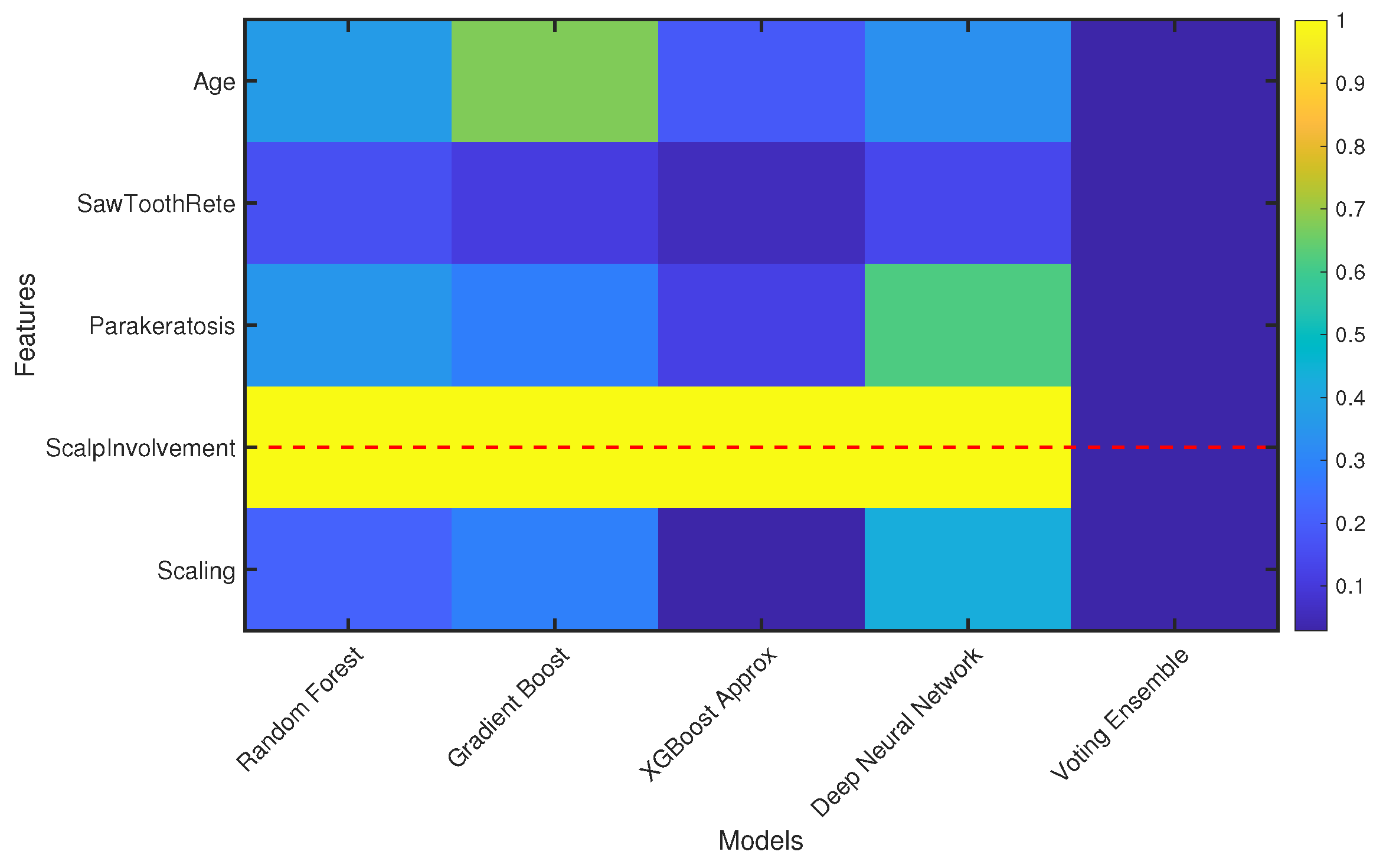
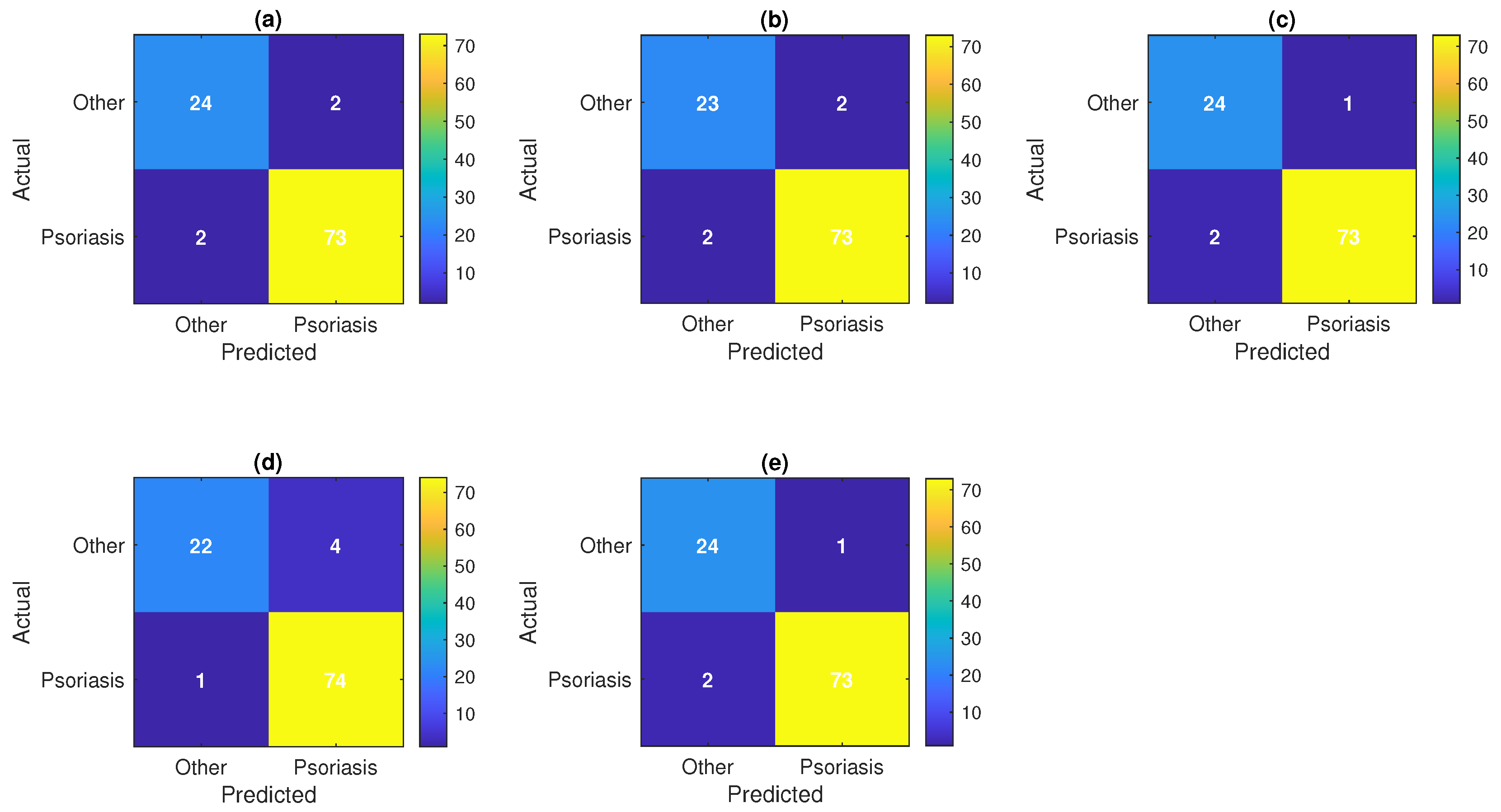
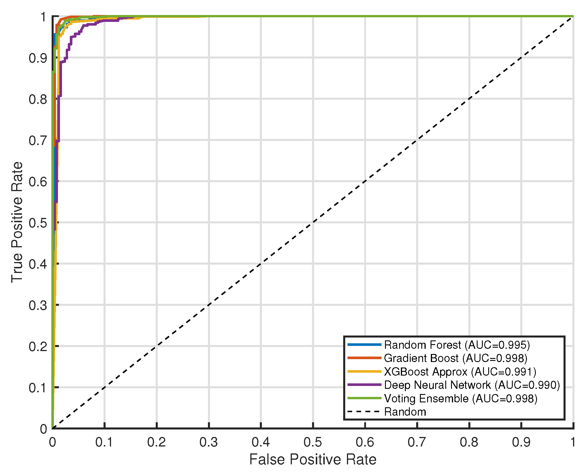
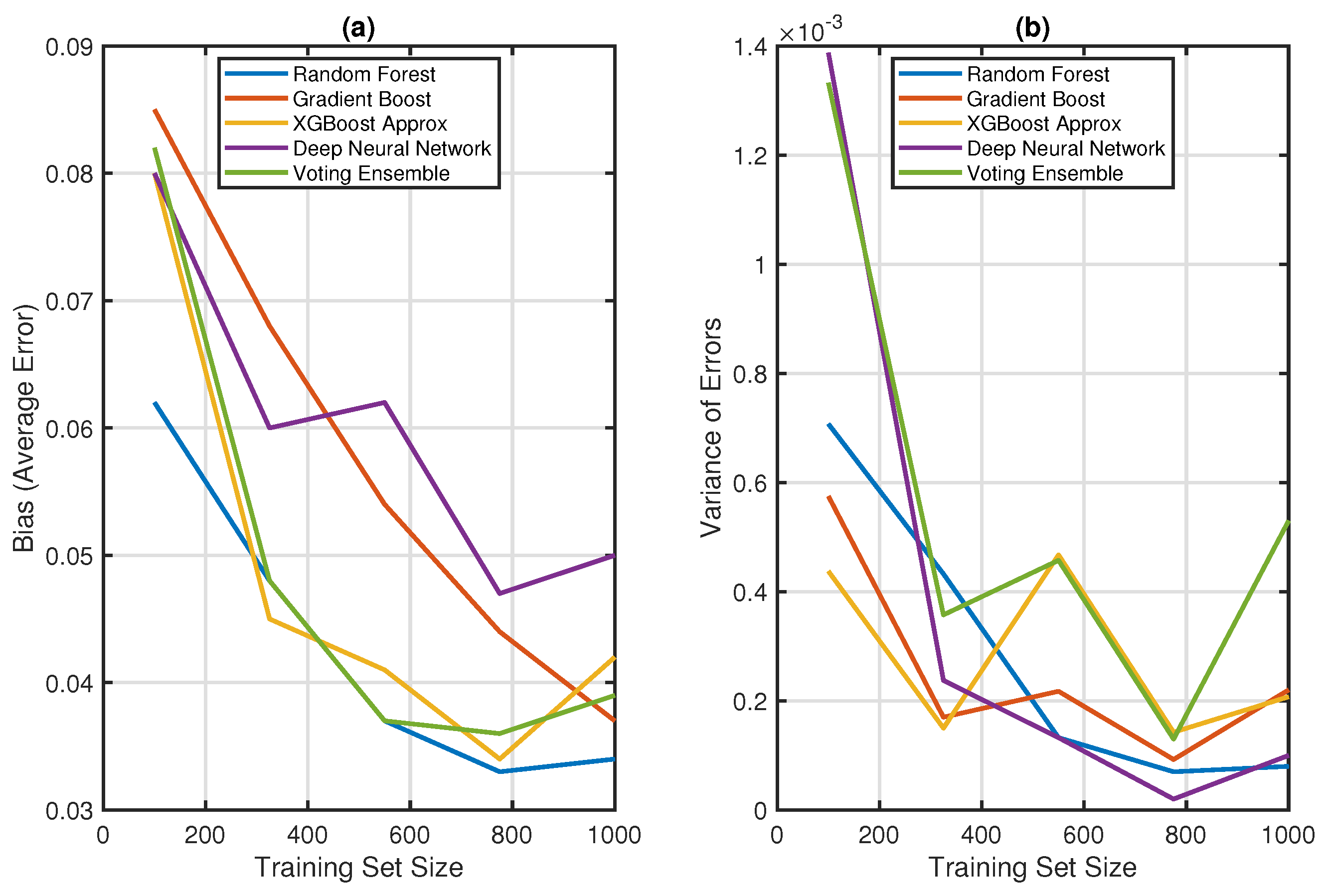
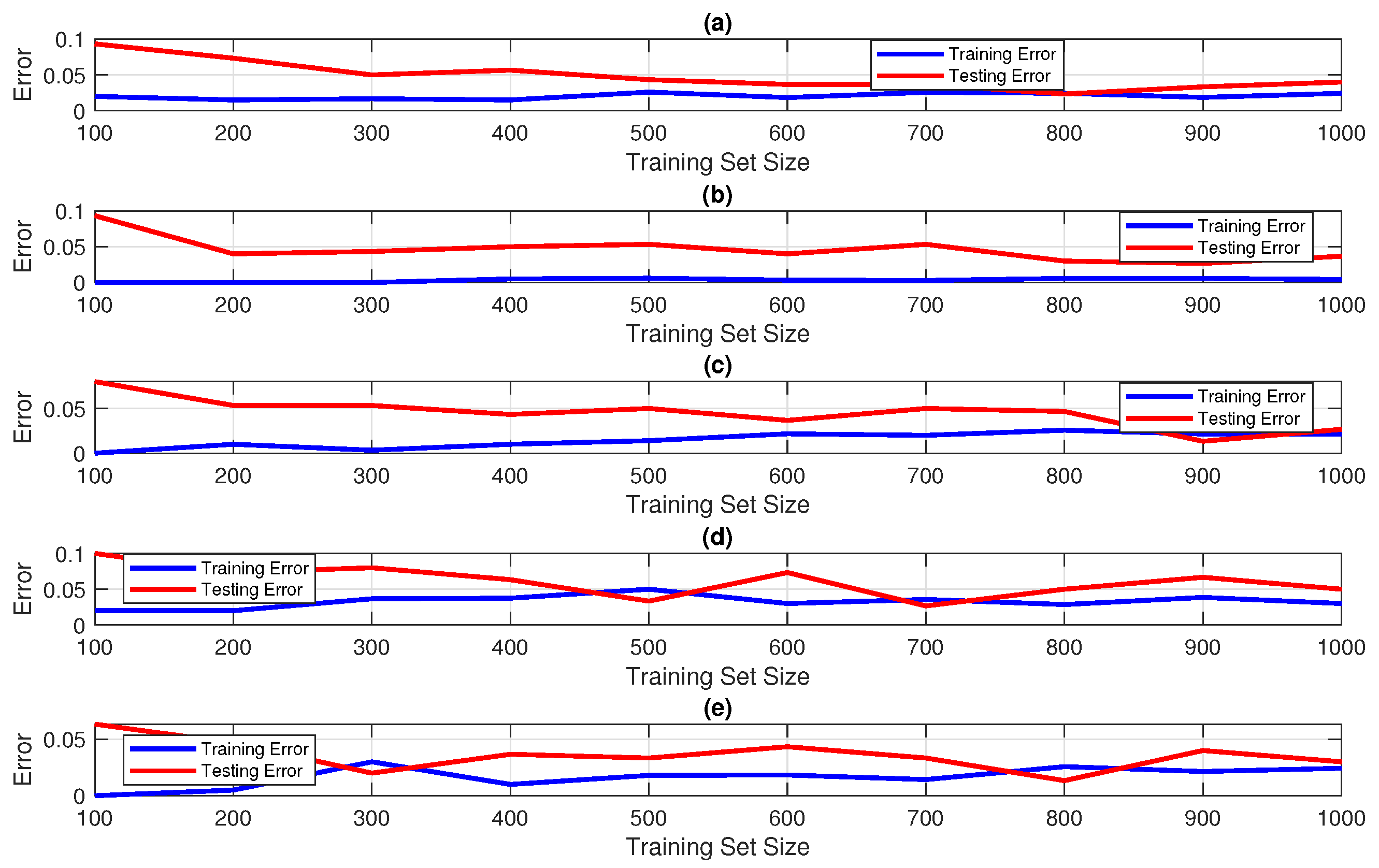
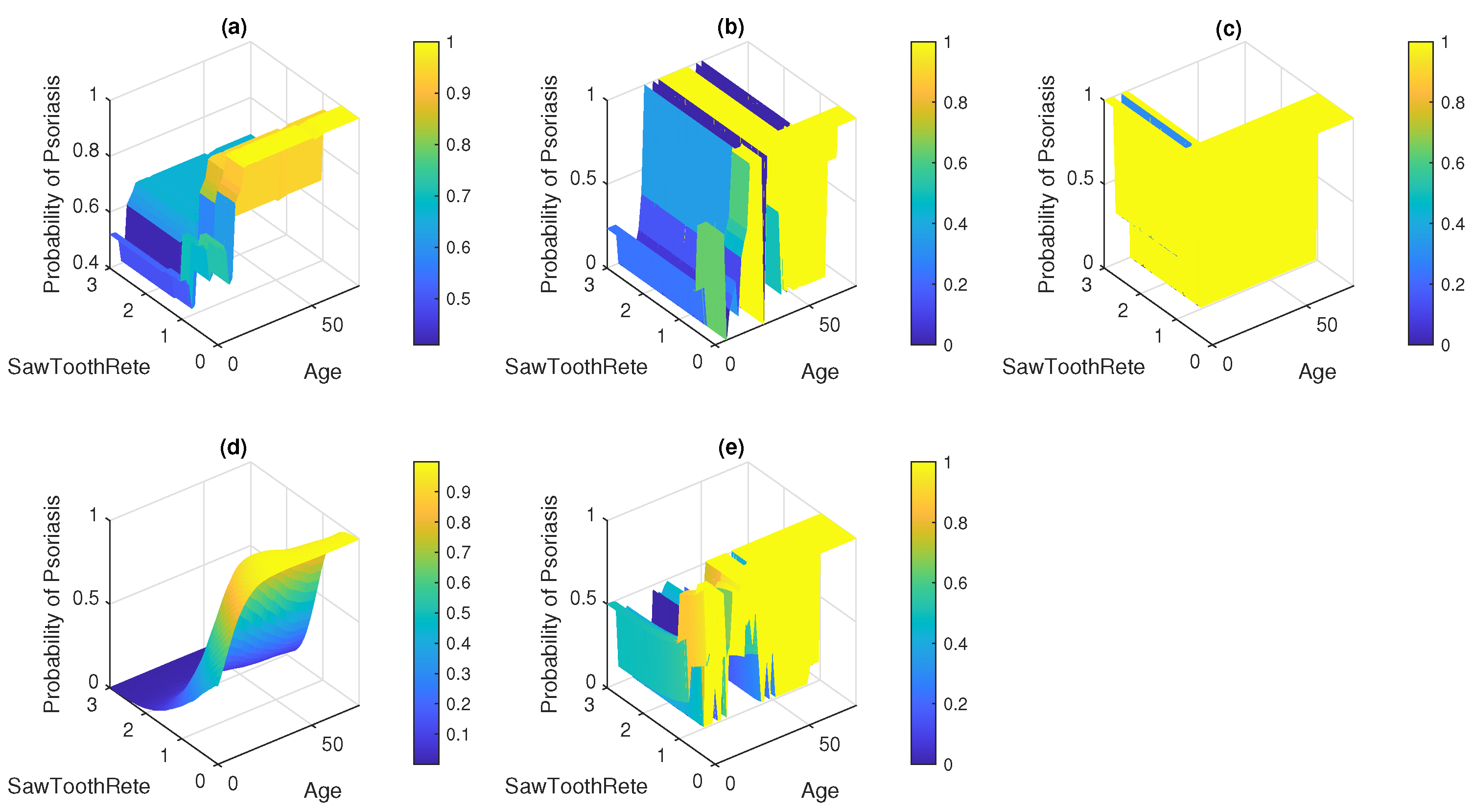
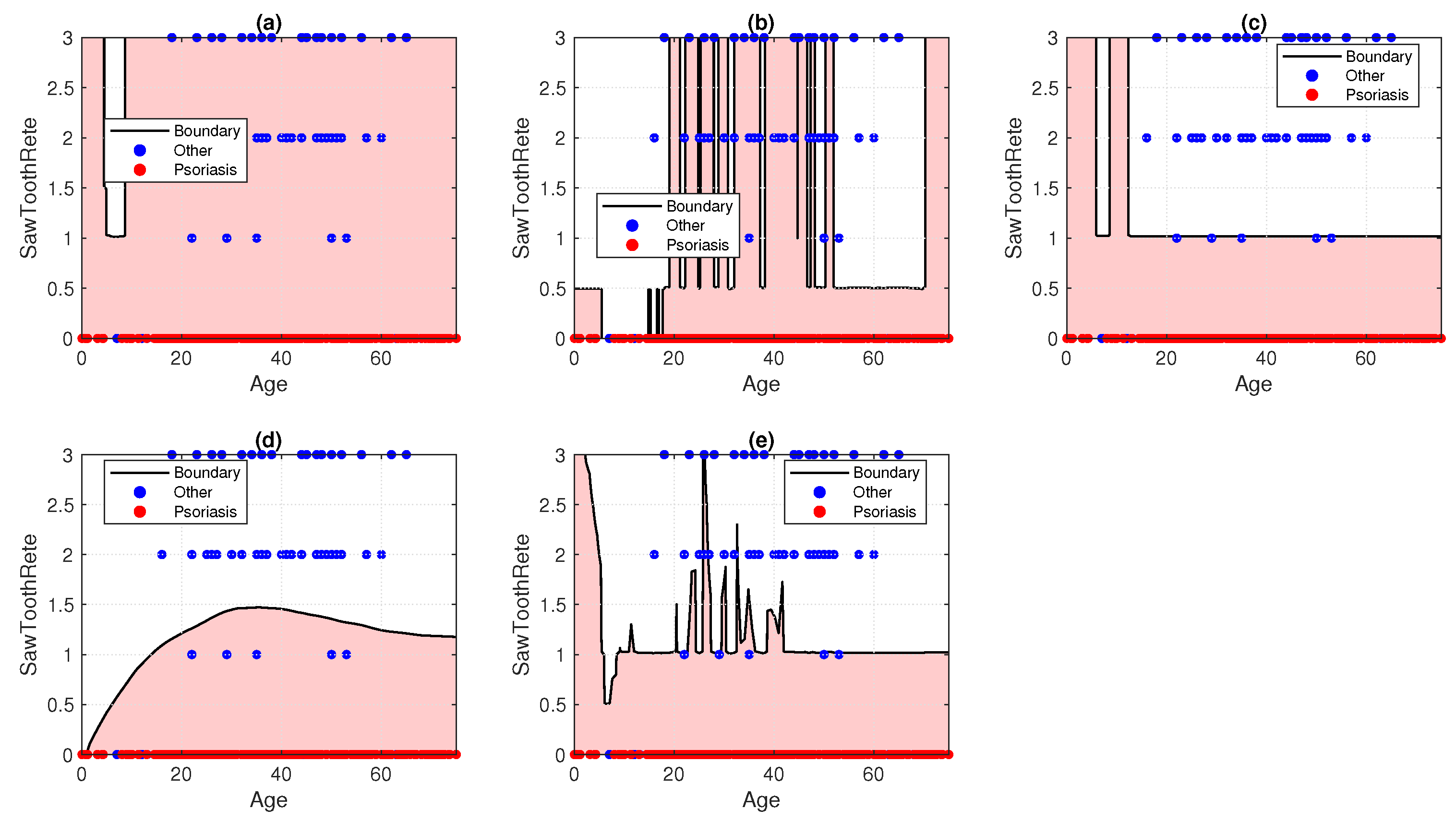
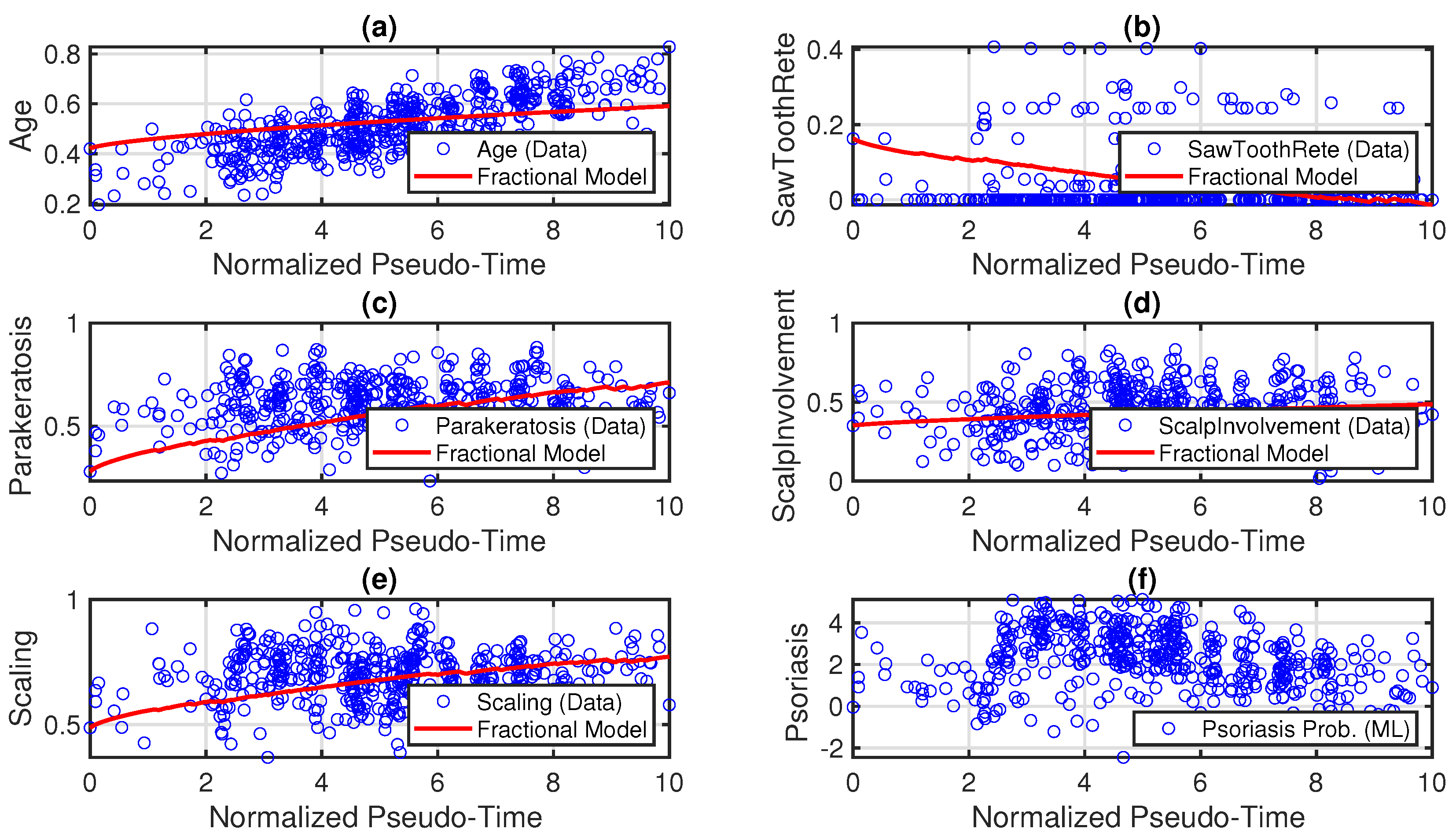
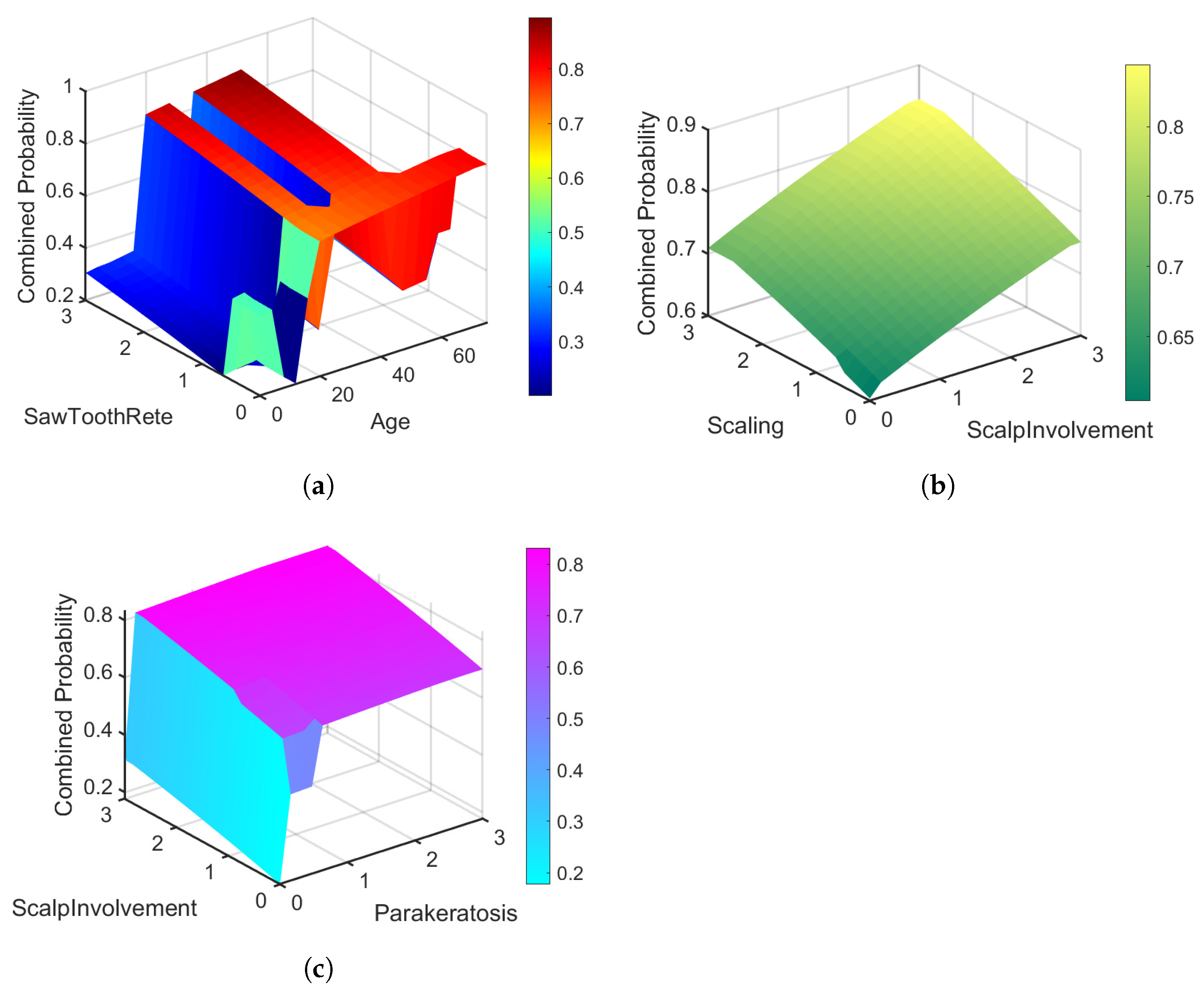
The study leverages the UCI Dermatology Dataset, starting with an analysis of feature distributions shown in Figure 2. These plots highlight the density variations of key features, Age, SawToothRete, Parakeratosis, Scalp Involvement, and Scaling across psoriasis and other conditions. For instance, Age shows a wider spread in non-psoriasis cases, indicating potential preprocessing needs to address skewness. The dataset summary in Table 1 provides further context: it includes 366 instances with 34 attributes and 6 classes, where psoriasis accounts for 30.60% of cases. Oversampling to 1000 instances using SMOTE helps balance this, with the top five features (Age, SawToothRete, Parakeratosis, Scalp Involvement, and Scaling) selected after handling missing values via median imputation, all sourced from the UCI repository. The Gradient Boost model’s feature importance, depicted in Figure 3, underscores the significant roles of SawToothRete and Parakeratosis in predicting psoriasis, reflecting their clinical relevance. Confusion matrices in Figure 4 further evaluate model performance, with XGBoost Approx. and Voting Ensemble showing strong results, 73 and 74 true positives for psoriasis, respectively, compared to the Deep Neural Network’s higher false negatives. These findings align with the cross-validated metrics in Table 3, where XGBoost Approx. leads with an accuracy of 0.972 ± 0.010 and an F1 score of 0.981 ± 0.007, while the Voting Ensemble excels in precision (0.986 ± 0.007) and AUC (0.992 ± 0.005), highlighting the strength of ensemble approaches. The ROC curves in Figure 5 reinforce this, with AUC values nearing 0.998 for Gradient Boost and Voting Ensemble, indicating excellent separation of psoriasis cases across thresholds, a critical factor for clinical reliability. Bias-variance analysis in Figure 6 shows the Voting Ensemble maintaining the lowest combined error as training size grows, suggesting good generalization, unlike the Deep Neural Network’s higher variance at smaller datasets. Learning curves in Figure 7 support this, with XGBoost Approx. and Voting Ensemble converging training and testing errors beyond 600 samples, indicating efficient learning from the oversampled data. Probability surfaces in Figure 8 illustrate psoriasis likelihood across Age and SawToothRete, with the Voting Ensemble offering smoother gradients and higher confidence in high-risk areas, smoothing out the sharper boundaries seen in Random Forest. Decision boundaries in Figure 9 further clarify this, with Gradient Boost providing an elaborate separation that aligns with data clusters, reflecting its ability to capture feature interactions key to psoriasis. The integration of ML with fractional-order modeling is detailed in Table 4, where state variables S 1 to S 5 are coupled via coefficients c 1 to c 7 and modulated by the fractional order β , which accounts for memory effects in disease progression. Optimization results in Table 5 show growth rates g set at 0.0500 and β at 0.6781 after 54 iterations, achieving a weighted MSE of 0.0031, confirming a strong fit to the data. The optimized fractional order β = 0.6781 reflects the non-integer dynamics inherent to psoriasis, where β < 1 indicates sub-diffusive processes characteristic of memory effects in chronic inflammation. Biologically, this value corresponds to the disease’s chronicity, as psoriasis involves prolonged epidermal turnover and immune memory from T-cell activation, where past inflammatory states (for example, cytokine accumulation) influence future flare-ups over extended timescales. In contrast to integer-order models ( β = 1 ), which assume instantaneous changes, this fractional order captures the hereditary properties of keratinocyte hyperproliferation and dermal infiltration, aligning with clinical observations of relapsing-remitting patterns in psoriasis patients. This interpretation is supported by similar applications in tumor growth models, where the fractional orders model persistent cellular memory. The fitted dynamics in Figure 10 compare the model’s trajectories to empirical data, with close tracking of Age (weight 0.249) and SawToothRete (0.230), demonstrating how fractional derivatives capture the gradual evolution of psoriasis probability over pseudo-time.
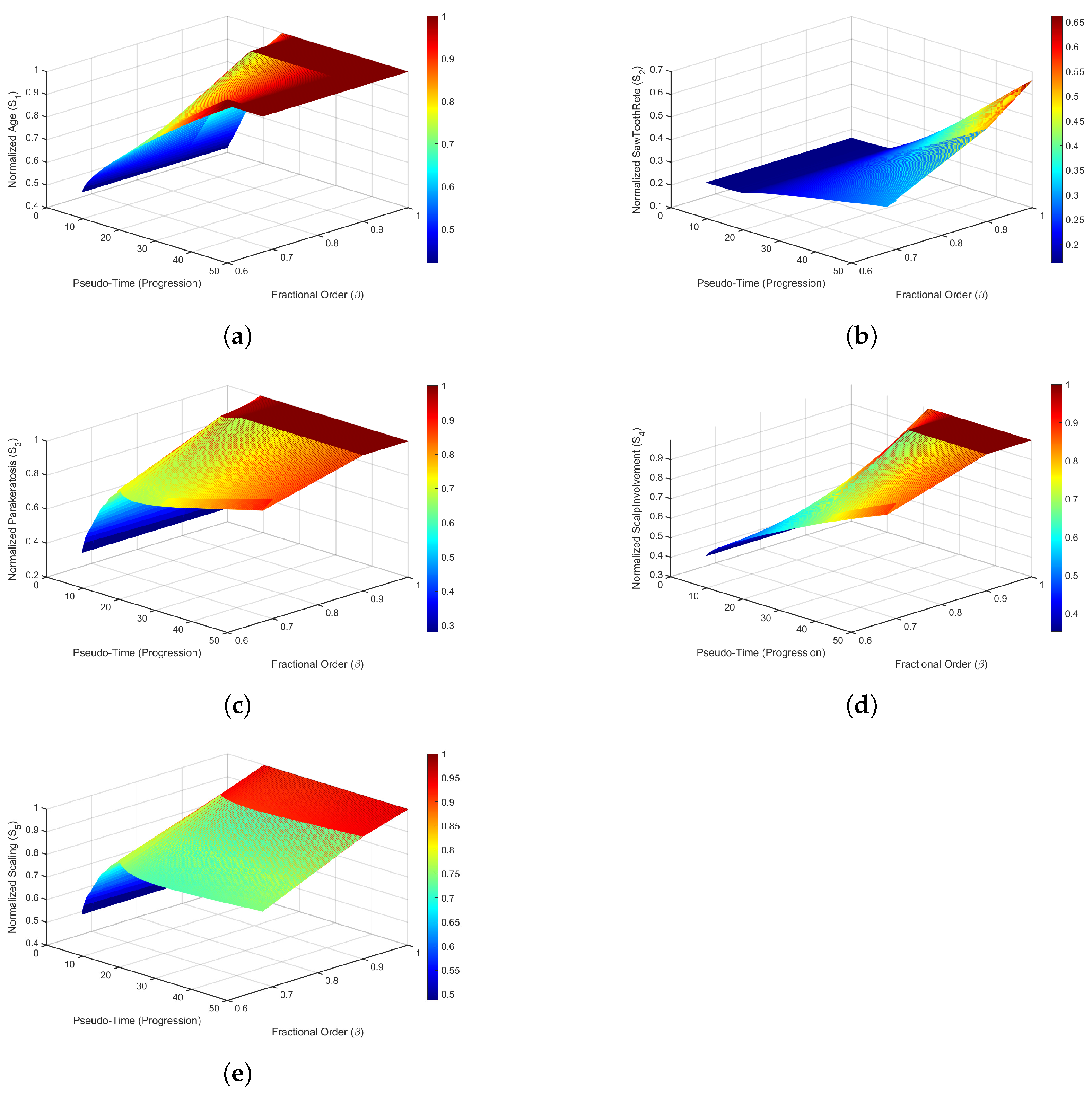
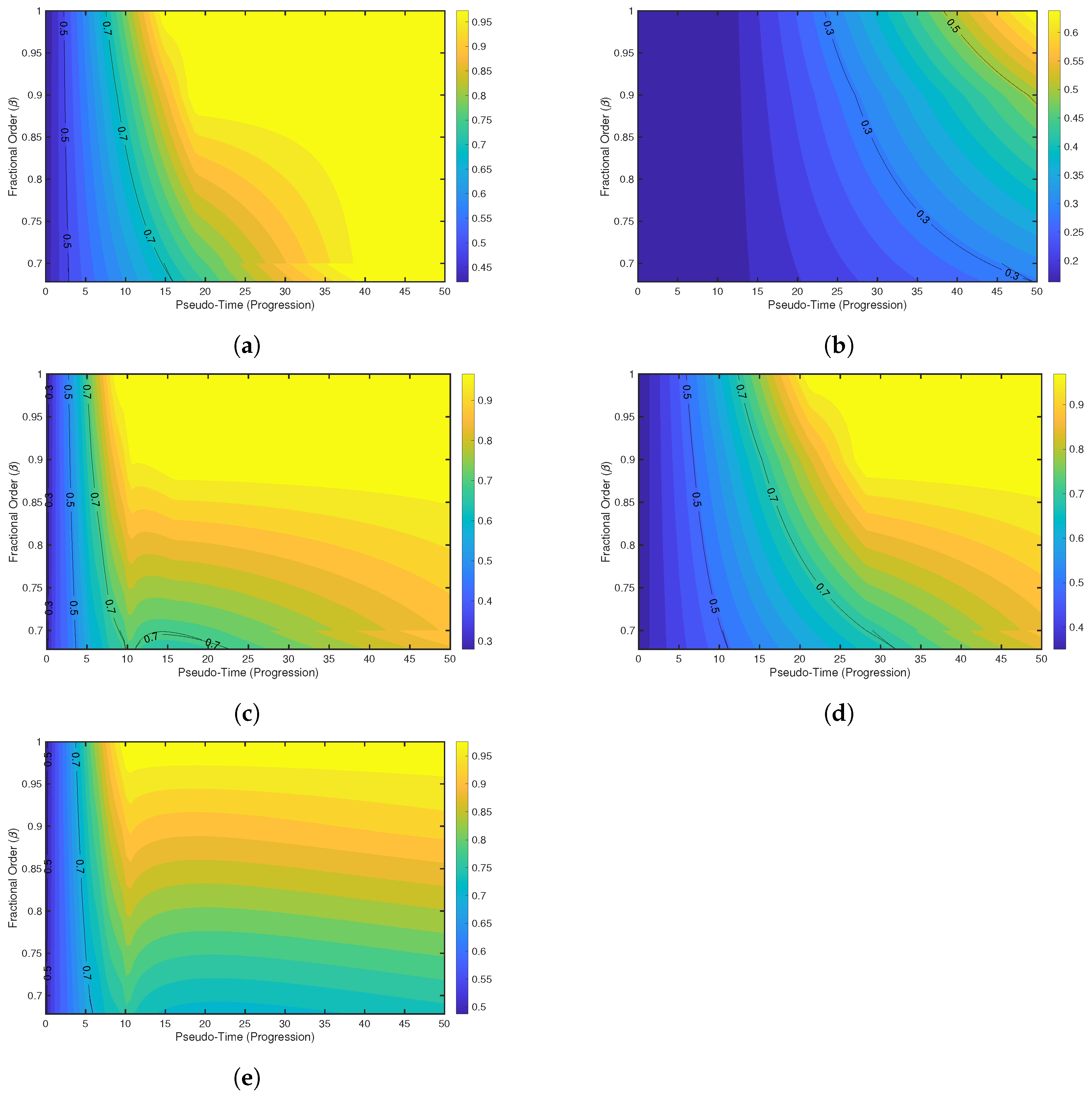
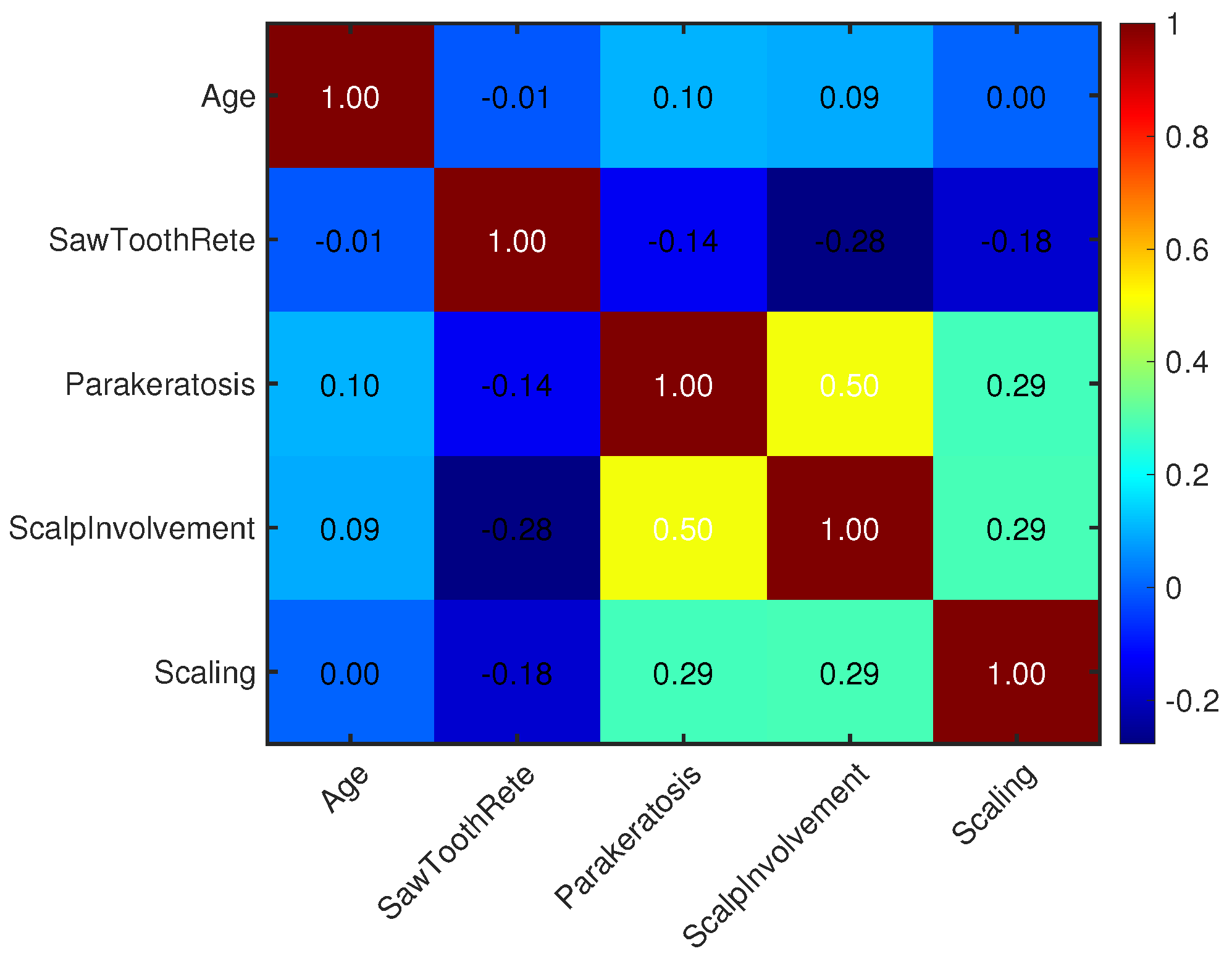
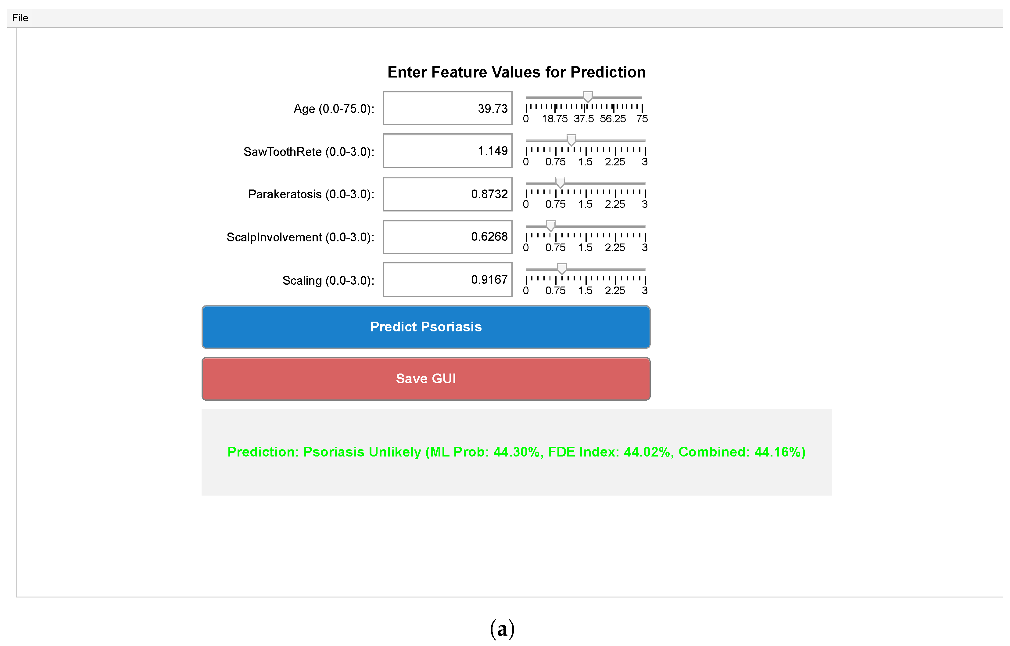
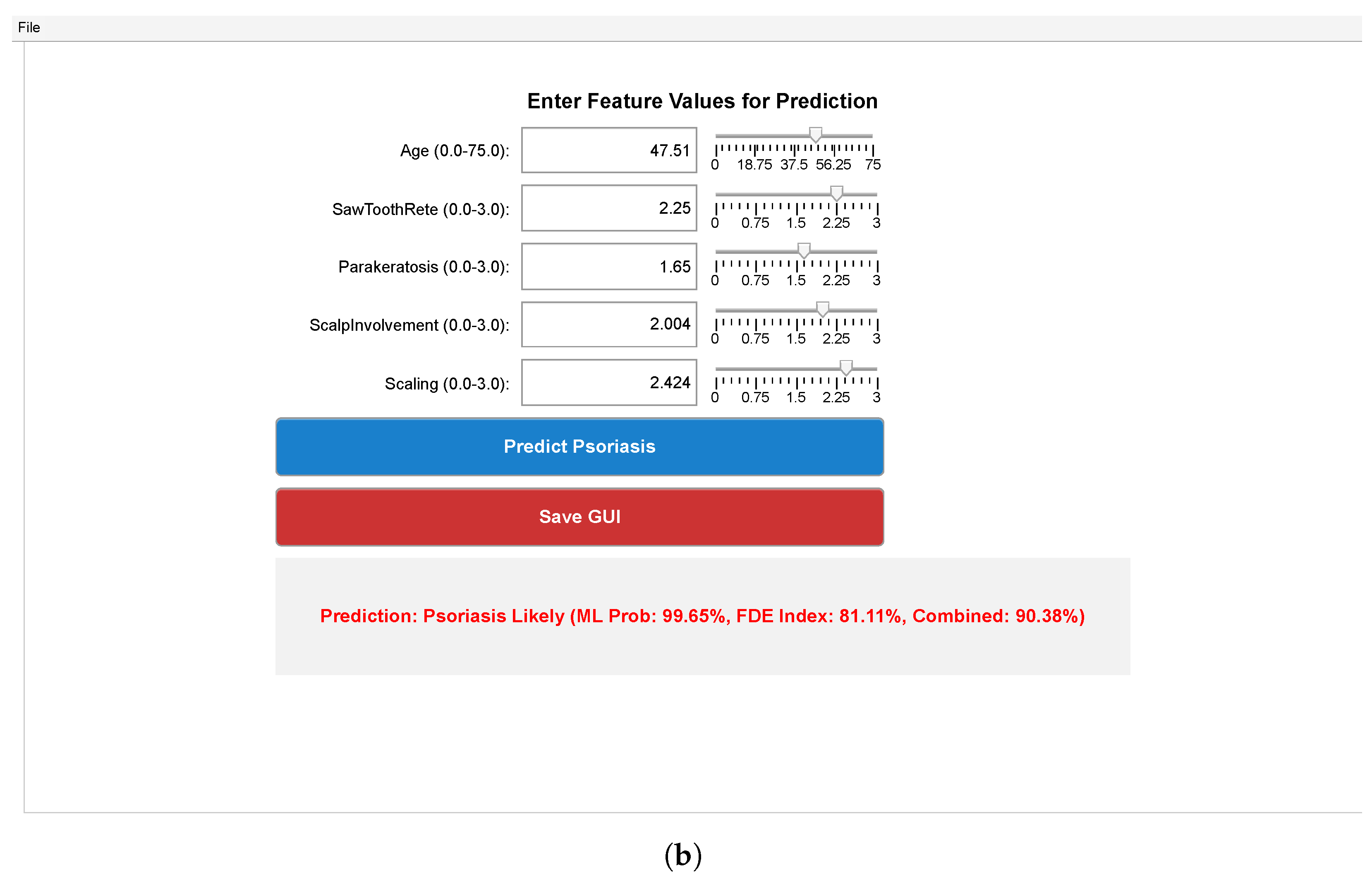
The feature ranges in Table 2 contextualize this, mapping raw values to normalization, ensuring stability and interpretability. Surface plots in Figure 11 reveal how state variables like S 3 (Parakeratosis) rise with higher β , suggesting fractional memory enhances the persistence of inflammatory markers. Contour plots in Figure 12 refine this, showing stable plateaus for S1 (Age) beyond pseudo-time 20, offering insights into long-term disease trends. Feature correlations in Figure 13 highlight a 0.50 link between Parakeratosis and Scalp Involvement, informing FDE coupling terms and explaining Gradient Boost’s robustness. Combined ML-FDE predictions in Figure 14 integrate probabilities across feature pairs, providing an elaborate risk assessment, especially in transitional zones. The GUI in Figure 15a brings this to life, with one case predicting low psoriasis likelihood (44.16% combined) for moderate inputs and another high (90.38%) for elevated values, fulfilling the study’s goal of delivering real-time, integrated diagnostics. The results breathe new life into dermatology diagnostics by seamlessly blending ML and FDE approaches. The XGBoost Approx. and Voting Ensemble models stand out, delivering near-perfect AUCs and robust confusion matrix outcomes, which translate into reliable predictions even with imbalanced data. This is particularly exciting, as it suggests these models can handle the complexity of real-world dermatological data, where psoriasis often presents with subtle variations. The fractional-order model adds a dynamic layer, with its fitted trajectories in Figure 10 mirroring empirical trends and the optimized β of 0.6781 capturing the memory effects of disease progression, something traditional models often fail at. The optimized fractional order models sub-diffusive processes in psoriasis, reflecting memory effects from chronic inflammation, long-term tissue remodeling, and disease chronicity, where past states influence current progression more than in integer-order models. This integration shines in the GUI (Figure 15), where clinicians can input patient data and receive instant, evidence-based risk assessments, like the stark contrast between a 44.16% and 90.38% probability, empowering timely interventions. The surface and contour plots (Figure 11 and Figure 12) reveal how fractional order influences state variables, with Parakeratosis showing heightened sensitivity that could guide targeted therapies. The strong correlation between Parakeratosis and Scalp Involvement (Figure 13) further validates the FDE’s coupling structure, offering a deeper understanding of how these features evolve together. While the models perform admirably, challenges remain, such as ensuring generalization across diverse populations and refining the GUI for broader clinical adoption. Future work could explore larger datasets or additional features to enhance predictive power, but the current framework marks a significant step toward integrating advanced mathematics with practical healthcare solutions.
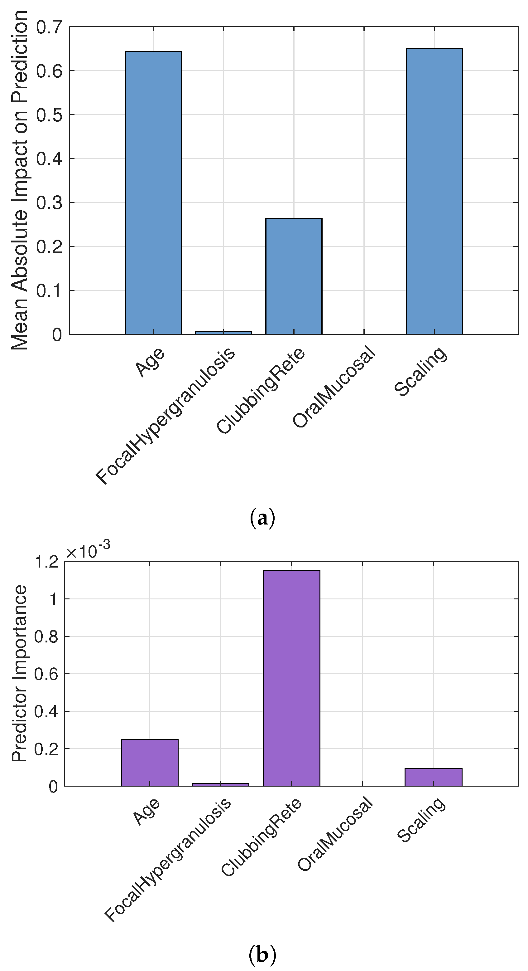
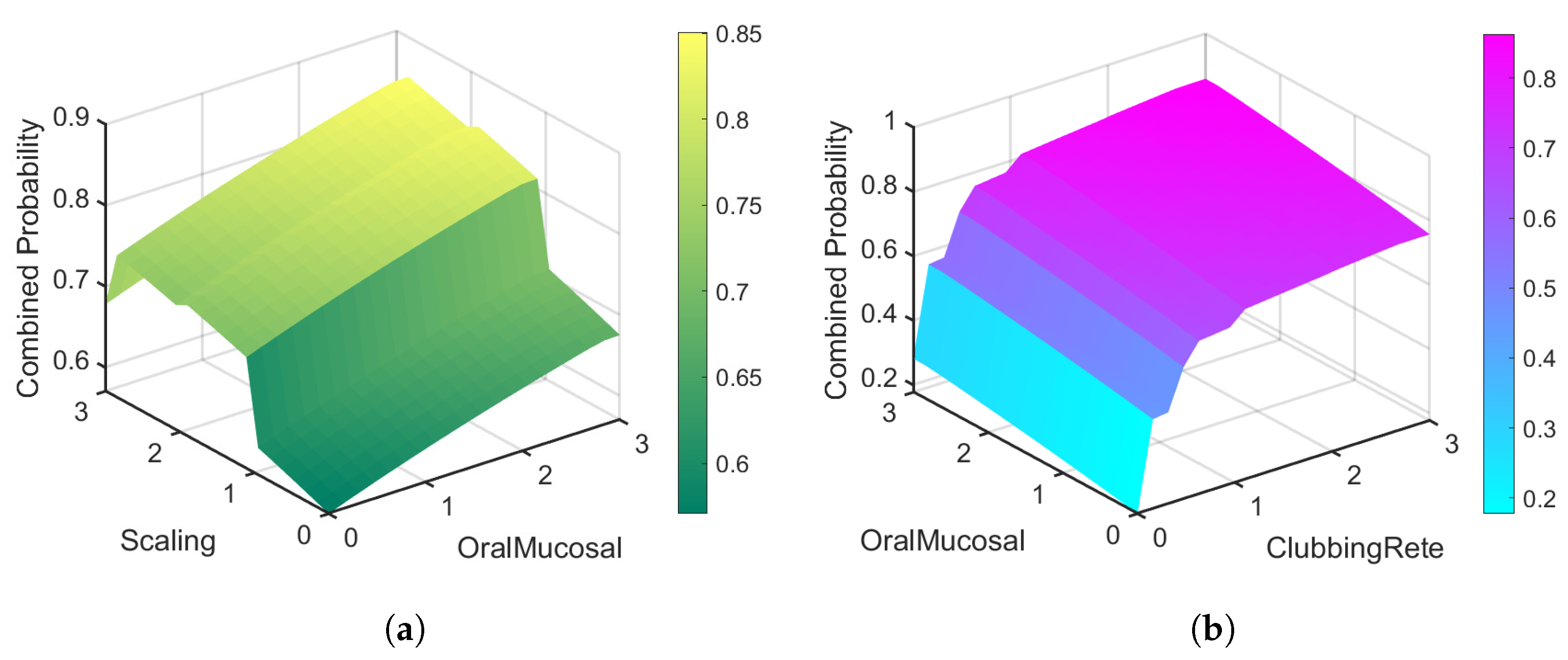
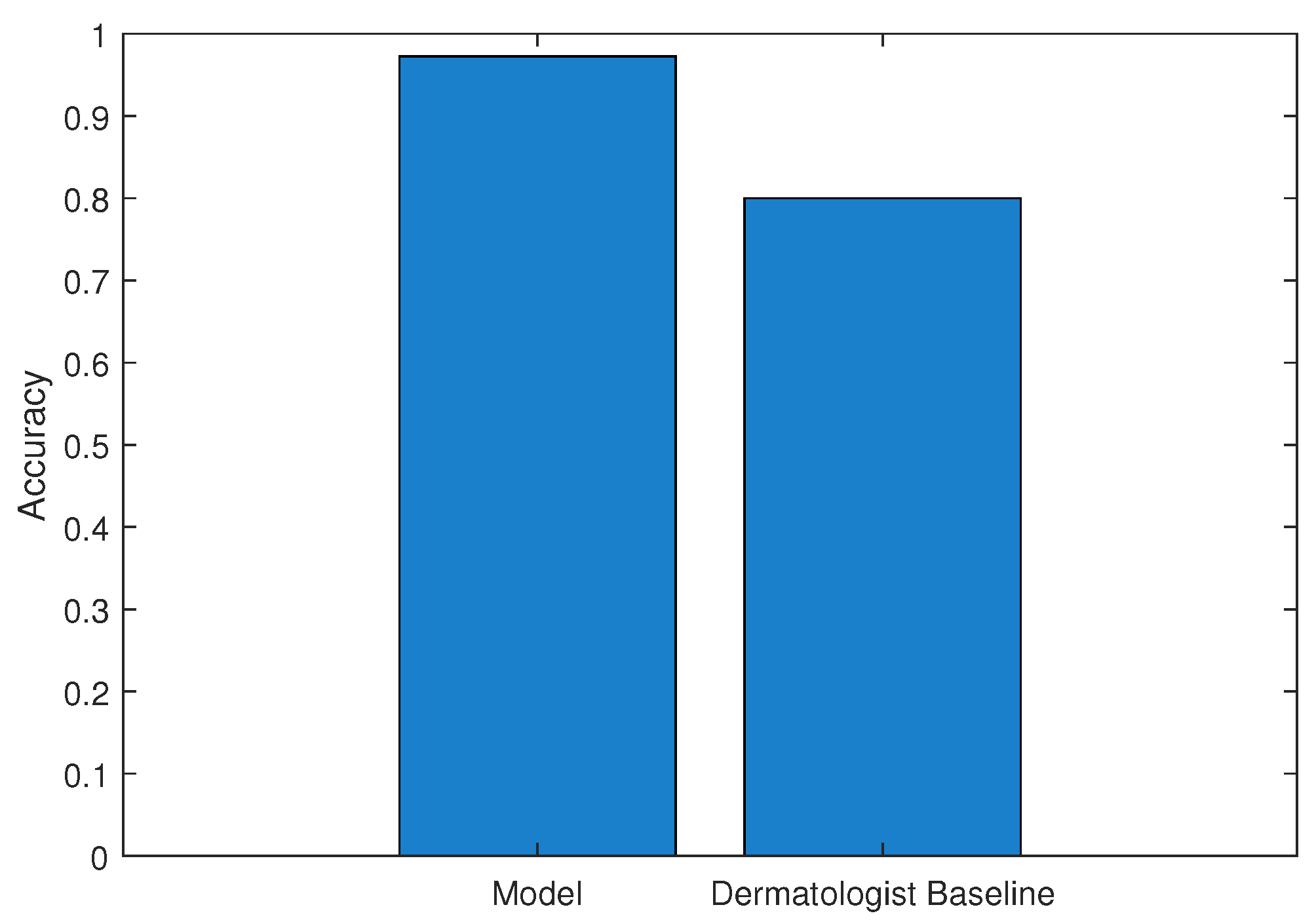
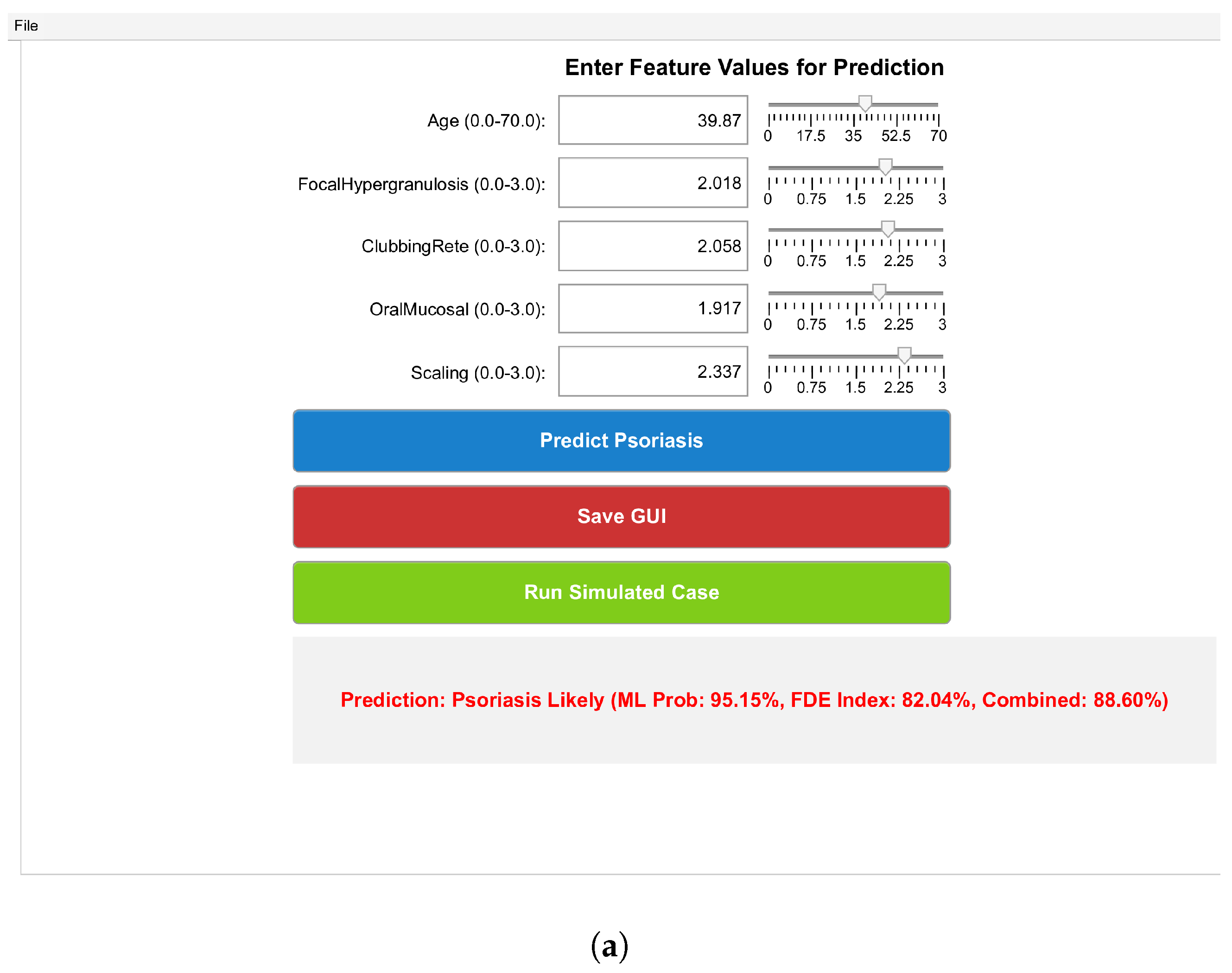
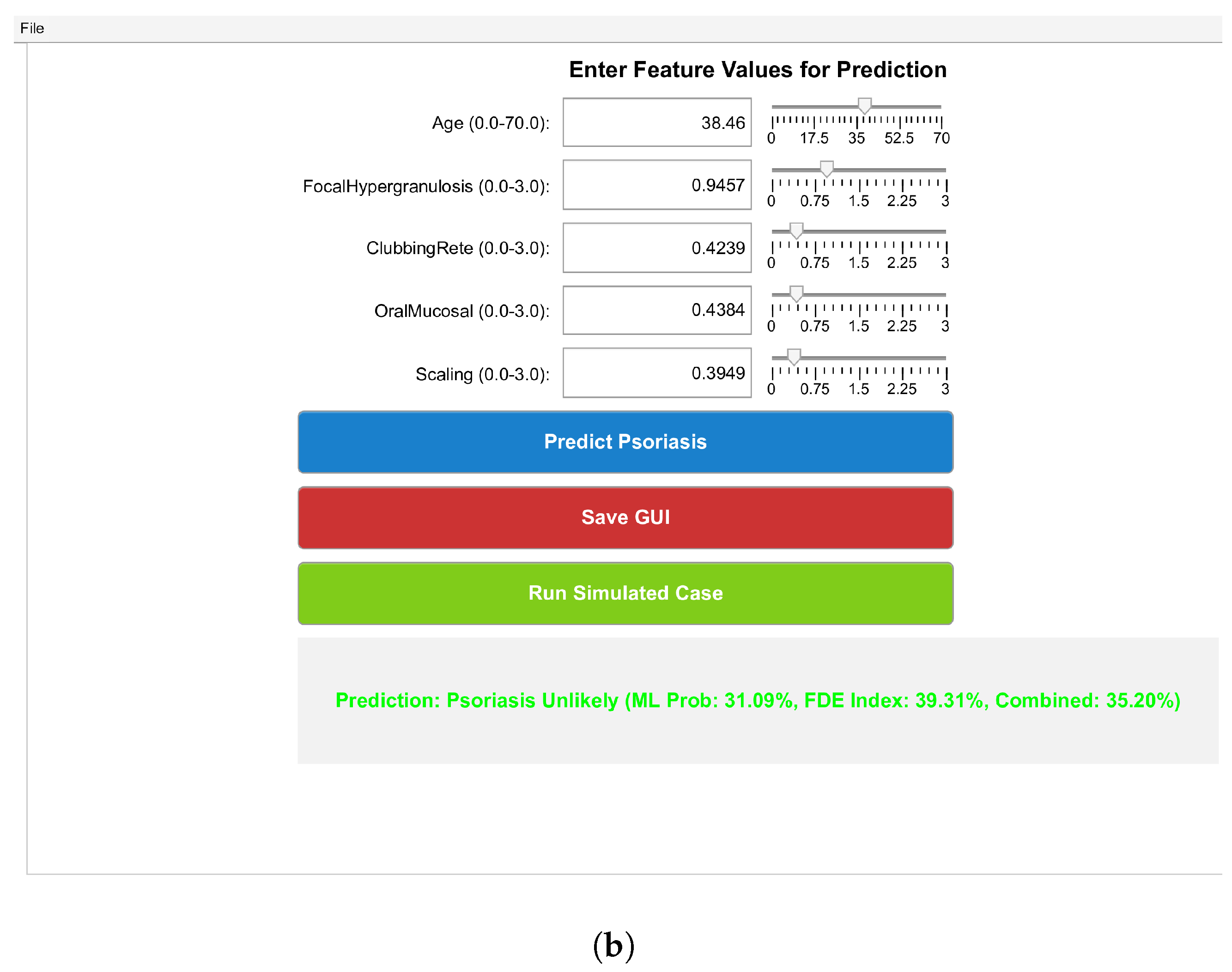
The local interpretability of the model is demonstrated through the SHAP analysis (Figure 16a) and LIME analysis (Figure 16b), which are presented in Figure 16. These analyses provide insights into feature contributions and local decision-making processes, enhancing the model’s transparency. More combined ML-FDE probabilities are visualized in Figure 17, showcasing the relationships between Scaling and OralMucosal (Figure 17a) and OralMucosal versus ClubbingRete (Figure 17b). These plots illustrate the predictive power of the integrated model across different feature combinations. A baseline comparison analysis, depicted in Figure 18, compares the model’s accuracy against a dermatologist baseline, highlighting the model’s competitive performance. To address generalizability, we implemented a stratified 80/20 hold-out validation, yielding an accuracy of 0.9726, precision of 0.9545, recall of 0.9545, F1 score of 0.9545, and AUC of 0.9831 on the test set. While this serves as pseudo-external validation, future work should incorporate independent clinical datasets from hospital records. More simulated cases via the Dermatology Diagnosis System GUI, which integrates ML-FDE predictions, are shown in Figure 19. This figure includes a case with a low likelihood of psoriasis (Figure 19a) and a case with a high likelihood (Figure 19b), demonstrating the system’s practical application and user interface. The GUI is designed for deployment on hospital systems via MATLAB Runtime, enabling clinicians to input patient features on standard interfaces. Practical implementation involves integration with electronic health records for seamless data flow. Validation is proposed through a pilot study with dermatologists, assessing usability and accuracy via feedback on several simulated cases, ensuring workflow compatibility and clinical trust.

8. Conclusions

This study advances dermatological diagnostics by pioneering the integration of machine learning predictions with fractional-order differential equations, offering a novel approach that captures the memory-dependent progression of psoriasis through real-world data from the UCI Dermatology Dataset. By informing the FDE parameters with optimized ML outputs and developing a user-friendly GUI for combined real-time predictions, the framework introduces a hybrid methodology that bridges computational efficiency with physiological realism, a departure from traditional integer-order models or standalone ML applications. The novelty lies in this seamless fusion, where ML-derived probabilities dynamically drive fractional dynamics, enabling more nuanced simulations of skin condition evolution that account for historical dependencies often overlooked in conventional analyses. The strengths of this research are evident in the robust performance of the ML models, particularly the Voting Ensemble’s superior precision and AUC, which enhance the reliability of inputs to the FDE system, resulting in accurate fittings and stable simulations. The fractional-order component provides enhanced modeling of long-term memory effects in disease pathways. At the same time, the GUI transforms complex computations into accessible tools for clinicians, potentially improving early detection and personalized treatment planning. The use of rigorous optimization and numerical methods ensures the framework’s applicability to public health scenarios, where timely and interpretable insights can inform policy and resource allocation. The dataset’s modest size and potential biases from oversampling, which may constrain generalizability to broader populations or rarer dermatological variants, may limit the study. Validation over several other independent datasets may strengthen assurance of the prediction outputs. The reliance on pseudo-time derived from age introduces assumptions that may not fully capture multifaceted disease triggers, and the computational demands of fractional solvers could hinder deployment in resource-limited settings without further optimization. Looking ahead, future directions could expand the framework by incorporating larger, multi-ethnic datasets or integrating multimodal data, such as imaging and genetic markers, to refine predictions. Exploring variable-order fractional derivatives might better adapt to varying disease stages, and partnering with healthcare providers for prospective trials could validate the GUI’s diagnostic utility. Ultimately, extending this hybrid approach to other chronic conditions, like autoimmune disorders, holds promise for broader impacts in precision medicine and epidemiological modeling.

Author Contributions

D.A.: Conceptualization, Data Curation, Methodology, Software, Formal analysis, Writing, and Original Draft. K.S.: Formal Analysis, Review, Visualization, Validation, and Project Administration. E.H.: Supervision, Review, and Editing. M.H.: Supervision, Review, and Editing. All authors have read and agreed to the published version of the manuscript.

Funding

This research received no external funding.

Institutional Review Board Statement

Not applicable.

Data Availability Statement

Data used in this study are referenced within the article.

Conflicts of Interest

The authors declare that they have no conflicts of interest to report regarding the present study.

References

  1. Alsararatee, H.H. Diagnostic tools and methods for dermatological assessment. Br. J. Nurs. 2025, 34, 502–512. [Google Scholar] [CrossRef] [PubMed]
  2. Patra, P.; Harrison, T.; Khoury, M. Challenges in diagnosis and treatment of pediatric psoriasis and atopic dermatitis. Arch. Dermatol. Res. 2025, 317, 393. [Google Scholar] [CrossRef]
  3. Lakum, M. The Hidden Struggle: Understanding the Psychosocial Impact of Dermatological Diseases. Indian J. Postgrad. Dermatol. 2024, 2, 74–79. [Google Scholar] [CrossRef]
  4. Parisi, R.; Iskandar, I.Y.; Kontopantelis, E.; Augustin, M.; Griffiths, C.E.; Ashcroft, D.M. National, regional, and worldwide epidemiology of psoriasis: Systematic analysis and modelling study. BMJ 2020, 369, m1590. [Google Scholar] [CrossRef]
  5. Dairov, A.; Issabekova, A.; Sekenova, A.; Shakhatbayev, M.; Ogay, V. Prevalence, incidence, gender and age distribution, and economic burden of psoriasis worldwide and in Kazakhstan. J. Clin. Med. Kazakhstan 2024, 21, 18–30. [Google Scholar] [CrossRef]
  6. Amiri, F.; Safiri, S.; Aletaha, R.; Mousavi, S.E.; Sullman, M.J.; Houshyar, Y.; Kolahi, A.-A.; Arshi, S. The Burden of Viral Skin Diseases in the Middle East and North Africa Region, 1990–2021. J. Infect. Public Health 2025, 18, 102784. [Google Scholar] [CrossRef] [PubMed]
  7. Fernandez-Figueras, M.T.; Puig, L. Histopathological diagnosis of psoriasis and psoriasiform dermatitides. Diagn. Histopathol. 2025, 31, 87–97. [Google Scholar] [CrossRef]
  8. Shehzadi, N.; Rehman, A.; Naz, S.; Rehman, S.; Khalifa, F. Machine learning and deep learning based psoriasis recognition system: Evaluation, management, prognosis—Where we are and the way to the future. Artif. Intell. Rev. 2025, 58, 263. [Google Scholar] [CrossRef]
  9. Khokhar, M.; Yadav, D.; Sharma, P. Transforming healthcare in the age of artificial intelligence: A new era of diagnostic excellence in laboratory medicine. Indian J. Clin. Biochem. 2025, 40, 163–164. [Google Scholar] [CrossRef] [PubMed]
  10. Sarker, M. Revolutionizing healthcare: The role of machine learning in the health sector. J. Artif. Intell. Gen. Sci. (JAIGS) 2024, 2, 36–61. [Google Scholar] [CrossRef]
  11. Hanna, M.G.; Pantanowitz, L.; Dash, R.; Harrison, J.H.; Deebajah, M.; Pantanowitz, J.; Rashidi, H.H. Future of artificial intelligence (AI)-machine learning (ML) trends in pathology and medicine. Mod. Pathol. 2025, 38, 100705. [Google Scholar] [CrossRef]
  12. AlSuwaidan, L. Deep learning based classification of dermatological disorders. Biomed. Eng. Comput. Biol. 2023, 14, 11795972221138470. [Google Scholar] [CrossRef]
  13. Virgens, G.S.; Teodoro, J.A.; Iarussi, E.; Rodrigues, T.; Amaral, D.T. Enhancing and advancements in deep learning for melanoma detection: A comprehensive review. Comput. Biol. Med. 2025, 194, 110533. [Google Scholar] [CrossRef]
  14. Sugiman, S.; Salman, S.; Catur, A.D.; Asmara, Y.P. Modelling the flexural properties of filled epoxy: Effects of volume fraction. E3s Web Conf. 2023, 465, 01028. [Google Scholar] [CrossRef]
  15. Dewi, D.A.; Thinakan, R.; Batumalay, M.; Kurniawan, T.B. A model for pervasive computing and wearable devices for sustainable healthcare applications. Int. J. Adv. Comput. Sci. Appl. 2023, 14, 527–530. [Google Scholar] [CrossRef]
  16. Acay, B.; Inc, M.; Khan, A.; Yusuf, A. Fractional methicillin-resistant Staphylococcus aureus infection model under Caputo operator. J. Appl. Math. Comput. 2021, 67, 755–783. [Google Scholar] [CrossRef]
  17. Karaca, Y. Computational complexity-based fractional-order neural network models for the diagnostic treatments and predictive transdifferentiability of heterogeneous cancer cell propensity. Chaos Theory Appl. 2023, 5, 34–51. [Google Scholar] [CrossRef]
  18. Abdeljawad, T.; Sher, M.; Shah, K.; Sarwar, M.; Amacha, I.; Alqudah, M.; Al-Jaser, A. Analysis of a class of fractal hybrid fractional differential equation with application to a biological model. Sci. Rep. 2024, 14, 18937. [Google Scholar] [CrossRef] [PubMed]
  19. Swain, S.; Swain, S.; Panda, B.; Tripathy, M.C. Modeling and optimal analysis of lung cancer cell growth and apoptosis with fractional-order dynamics. Comput. Biol. Med. 2025, 188, 109837. [Google Scholar] [CrossRef] [PubMed]
  20. Nagpurkar, M.B.; Kachhia, K.B. A novel numerical method for solving fractal-fractional differential equations with exponential memories. J. Appl. Math. Comput. 2025, 71, 1453–1475. [Google Scholar] [CrossRef]
  21. Saadeh, R.; Abdoon, M.A.; Qazza, A.; Berir, M.; Guma, F.E.; Al-Kuleab, N.; Degoot, A.M. Mathematical modeling and stability analysis of the novel fractional model in the Caputo derivative operator: A case study. Heliyon 2024, 10, e26611. [Google Scholar] [CrossRef] [PubMed]
  22. Banerjee, R.; Biswas, R.K. Mathematical Model of the Disease Psoriasis: An Optimal Control-Based Approach. In Control and Measurement Applications for Smart Grid: Select Proceedings of SGESC 2021; Springer Nature: Singapore, 2022; pp. 167–178. [Google Scholar] [CrossRef]
  23. Cao, X.; Datta, A.; Al Basir, F.; Roy, P.K. Fractional-order model of the disease psoriasis: A control based mathematical approach. J. Syst. Sci. Complex. 2016, 29, 1565–1584. [Google Scholar] [CrossRef]
  24. Roy, P.K.; Datta, A. Mathematical Models for Therapeutic Approaches to Control Psoriasis; Springer: Singapore, 2019. [Google Scholar] [CrossRef]
  25. Singh, A.; Chavada, A.; Pathak, N. Fractional Calculus Approach to Pancreatic Cancer Therapy: Modeling Tumor and Immune Interactions with siRNA Treatment. Int. J. Appl. Comput. Math. 2025, 11, 61. [Google Scholar] [CrossRef]
  26. Ahmed, S.; Ullah, S.; Riaz, M.; Ahmed, W.; Sheikh, M. Numerical Analysis of Fractional Logistic Growth Models Using Computational Methods with MATLAB Codes. Int. J. Appl. Comput. Math. 2025, 11, 198. [Google Scholar] [CrossRef]
  27. Wei, G.; Zhang, X.; Cui, Z. Primary resonance analysis of a novel fractional-order coronary artery model. Aims Math. 2025, 10, 14996–15011. [Google Scholar] [CrossRef]
  28. Amilo, D.; Sadri, K.; Hincal, E.; Farman, M.; Nisar, K.S. Dual approach artificial neural networks-fractional order operator to enhancing in vitro fertilization predictions and success measure. Model. Earth Syst. Environ. 2025, 11, 281. [Google Scholar] [CrossRef]
  29. Amilo, D.; Sadri, K.; Hincal, E. A hybrid approach to heart disease prediction using a fractional-order mathematical model and machine learning algorithm. Comput. Methods Biomech. Biomed. Eng. 2025, 1–30. [Google Scholar] [CrossRef]
  30. Amilo, D.; Sadri, K.; Hincal, E.; Farman, M.; Nisar, K.S.; Hafez, M. An integrated machine learning and fractional calculus approach to predicting diabetes risk in women. Healthc. Anal. 2025, 8, 100402. [Google Scholar] [CrossRef]
  31. Debelee, T.G. Skin lesion classification and detection using machine learning techniques: A systematic review. Diagnostics 2023, 13, 3147. [Google Scholar] [CrossRef]
  32. Raman, R.; Kumar, V.; Saini, D.; Rabadiya, D.; Patre, S.; Meenakshi, R. Machine Learning-Driven Approaches for Dermatological Disease Diagnosis. In Proceedings of the 2024 International Conference on Data Science and Network Security (ICDSNS), Tiptur, India, 26–27 July 2024; pp. 1–5. [Google Scholar] [CrossRef]
  33. Amini, M.; Vatankhah, R. The Effect of Disease Stage on Melanoma Treatment Efficacy: Insights from Mathematical Modeling and In vivo Clinical Data. Bull. Math. Biol. 2025, 87, 90. [Google Scholar] [CrossRef] [PubMed]
  34. Rodrigues, G.; Silva, J.; Santurio, D.S.; Mancera, P.F.A. A mathematical model to describe the melanoma dynamics under effects of macrophage inhibition and car t-cell therapy. Trends Comput. Appl. Math. 2024, 25, e01734. [Google Scholar] [CrossRef]
  35. Ilter, N.; Guvenir, H. Dermatology [Dataset]; UCI Machine Learning Repository: 1998. Available online: https://archive.ics.uci.edu/dataset/33/dermatology (accessed on 10 October 2025).
  36. Abu-Shady, M.; Kaabar, M.K. A generalized definition of the fractional derivative with applications. Math. Probl. Eng. 2021, 2021, 9444803. [Google Scholar] [CrossRef]
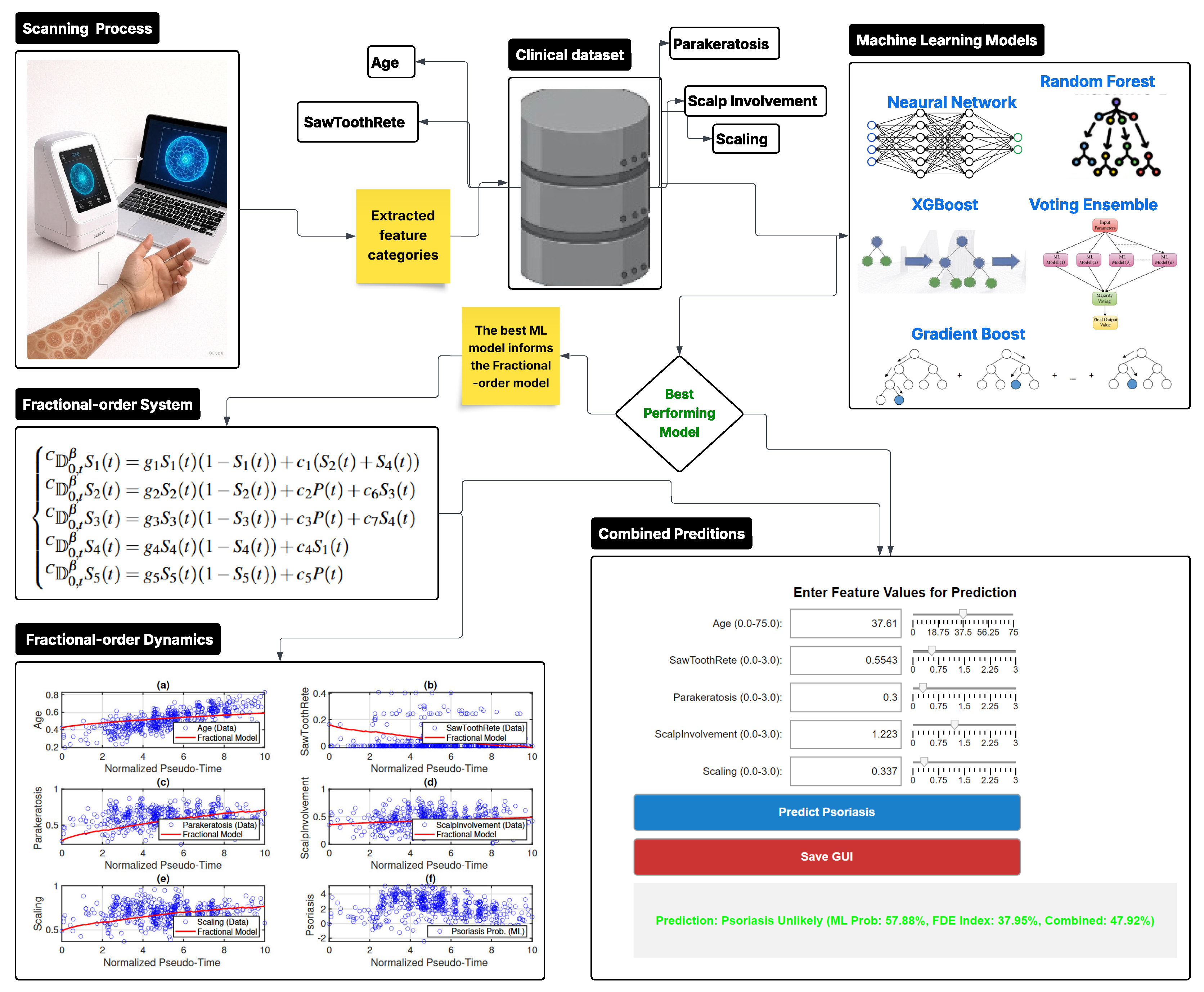
Figure 1. Schematic diagram of the hybrid machine learning and fractional-order differential equation framework for psoriasis prediction, depicting the integrated scanning process, data flow, model synchronization, and predictive outputs.
Appliedmath 05 00143 g001
Figure 2. Feature distributions.
Appliedmath 05 00143 g002
Figure 3. Feature importance.
Appliedmath 05 00143 g003
Figure 4. Confusion matrix: (a) Random Forest, (b) Gradient Boost, (c) XGBoost Approx., (d) Deep Neural Network, and (e) Voting Ensemble.
Appliedmath 05 00143 g004
Figure 5. ROC curve.
Appliedmath 05 00143 g005
Figure 6. Bias-variance analysis.
Appliedmath 05 00143 g006
Figure 7. Learning curves: (a) Random Forest, (b) Gradient Boost, (c) XGBoost Approx., (d) Deep Neural Network, and (e) Voting Ensemble.
Appliedmath 05 00143 g007
Figure 8. Probability surface: (a) Random Forest, (b) Gradient Boost, (c) XGBoost Approx., (d) Deep Neural Network, and (e) Voting Ensemble.
Appliedmath 05 00143 g008
Figure 9. Decision Boundary using SawToothRete versus Age: (a) Random Forest, (b) Gradient Boost, (c) XGBoost Approx., (d) Deep Neural Network, and (e) Voting Ensemble.
Appliedmath 05 00143 g009
Figure 10. Fitted dynamics of the fractional-order model compared to the empirical dataset with normalization: (a) Age (weight = 0.249), (b) SawToothRete Dynamics (weight = 0.230), (c) Parakeratosis Dynamics (weight = 0.054), (d) Scalp Involvement (weight = 0.224), (e) Scaling (weight = 0.223), and (f) Psoriasis Probability.
Appliedmath 05 00143 g010
Figure 11. Surface plots for state variables S i , i = 1 , 2 , , 5 in model (1), over pseudo-time and fractional-order: (a) S 1 Age, (b) S 2 (SawToothRete), (c) S 3 (Parakeratosis), (d) S 4 (Scalp Involvement), and (e) S 5 (Scaling).
Appliedmath 05 00143 g011
Figure 12. Contour plots for state variables S i , i = 1 , 2 , , 5 in model (1), over pseudo-time and fractional-order: (a) S 1 Age, (b) S 2 (SawToothRete), (c) S 3 (Parakeratosis), (d) S 4 (Scalp Involvement), and (e) S 5 (Scaling).
Appliedmath 05 00143 g012
Figure 13. Feature Correlation plot.
Appliedmath 05 00143 g013
Figure 14. Combined ML-FDE Probability Plots (a) Age versus SawToothRete, (b) Scaling versus Scapinvolvment, and (c) Parakeratosis versus Scapinvolvment.
Appliedmath 05 00143 g014
Figure 15. Dermatology Diagnosis System GUI integrating machine learning and fractional differential equation models: (a) a case predicting low likelihood of psoriasis, and (b) a case predicting high likelihood of psoriasis.
Appliedmath 05 00143 g015aAppliedmath 05 00143 g015b
Figure 16. Local Interpretability Analysis: (a) SHAP analysis, and (b) LIME analysis.
Appliedmath 05 00143 g016
Figure 17. Combined ML-FDE Probabilities: (a) Scaling versus OralMucosal, and (b) OralMucosal versus clubblingRete.
Appliedmath 05 00143 g017
Figure 18. Baseline Comparison Analysis.
Appliedmath 05 00143 g018
Figure 19. Dermatology Diagnosis System GUI integrating ML-FDE: (a) a case predicting low likelihood of psoriasis, and (b) a case predicting high likelihood of psoriasis.
Appliedmath 05 00143 g019aAppliedmath 05 00143 g019b
Table 1. Dataset Summary (UCI Dermatology Dataset).
ParameterValue
Number of Instances366
Number of Attributes34
Number of Classes6
Class Distribution (Psoriasis)30.60%
Oversampled Instances1000
Top Selected Features5
Feature NamesAge, SawToothRete, Parakeratosis, Scalp Involvement,
Scaling
Missing ValuesHandled by median imputation
Dataset SourceUCI Dermatology Dataset [35]
Table 2. Normalized Features and Estimated Raw Value Ranges from UCI Dermatology Dataset.
FeatureStateTypical Raw RangeNormalized Range
Age S 1 [ 0 , 100 ] [ 0 , 1 ]
Scaling S 2 [ 0 , 3 ] [ 0 , 1 ]
Erythema S 3 [ 0 , 3 ] [ 0 , 1 ]
Parakeratosis S 4 [ 0 , 3 ] [ 0 , 1 ]
Scalp Involvement S 5 [ 0 , 3 ] [ 0 , 1 ]
Table 3. Cross-Validated Performance (Mean ± Std) Across 10-Fold Cross-Validation. The best scores are highlighted in blue.
ModelAccuracyPrecisionRecallF1 ScoreAUC
XGBoost Approx0.972 ± 0.0100.984 ± 0.0080.979 ± 0.0090.981 ± 0.0070.984 ± 0.006
Voting Ensemble0.969 ± 0.0120.986 ± 0.0070.972 ± 0.0110.979 ± 0.0080.992 ± 0.005
Random Forest0.968 ± 0.0110.977 ± 0.0090.980 ± 0.0080.979 ± 0.0070.986 ± 0.006
Gradient Boost0.957 ± 0.0130.969 ± 0.0100.973 ± 0.0090.971 ± 0.0080.974 ± 0.007
Deep Neural Network0.955 ± 0.0150.952 ± 0.0120.989 ± 0.0060.970 ± 0.0090.975 ± 0.008
Table 4. Summary of variables and parameters in the fractional-order model.
SymbolDescription
S 1 ( t ) Normalized Age feature
S 2 ( t ) Normalized SawToothRete feature
S 3 ( t ) Normalized Parakeratosis feature
S 4 ( t ) Normalized Scalp Involvement feature
S 5 ( t ) Normalized Scaling feature
P ( t ) Machine learning-predicted psoriasis probability at pseudo-time t
g 1 , g 2 , g 3 , g 4 , g 5 Growth rates for each state variable S i (dimensionless)
c 1 Coupling coefficient from S 2 + S 4 to S 1 (dimensionless)
c 2 Coupling coefficient from P ( t ) to S 2 (dimensionless)
c 3 Coupling coefficient from P ( t ) to S 3 (dimensionless)
c 4 Coupling coefficient from S 1 to S 4 (dimensionless)
c 5 Coupling coefficient from P ( t ) to S 5 (dimensionless)
c 6 Coupling coefficient from S 3 to S 2 (dimensionless)
c 7 Coupling coefficient from S 4 to S 3 (dimensionless)
β Fractional order of the derivative (between 0 and 1)
Table 5. Summary of Gradient Boost optimization of the fractional-order model parameters using the Dermatology Dataset.
PropertyValue
Dataset Size (Original)366 samples, 34 features
Class Distribution30.60% psoriasis cases
Dataset Size (After Oversampling)1000 instances
Selected FeaturesAge, SawToothRete, Parakeratosis, Scalp Involvement, Scaling
Iterations54
Function Evaluations774
Final Objective Value (Fval) 3.050863 × 10 3
Feasibility 0.000
Final Step Length 0.000
Final Norm of Step 0.000
Final First-order Optimality 1.324 × 10 7
Stopping CriteriaStep size tolerance satisfied, constraints met
Optimized Parameter g[0.0500, 0.0500, 0.0500, 0.0500, 0.0500]
Optimized Parameter c[0.0413, –0.0423, 0.0684, 0.0252, 0.0509, 0.0012, 0.0280]
Optimized Parameter β 0.6781
Minimum Cost (Weighted MSE)0.0031
Disclaimer/Publisher’s Note: The statements, opinions and data contained in all publications are solely those of the individual author(s) and contributor(s) and not of MDPI and/or the editor(s). MDPI and/or the editor(s) disclaim responsibility for any injury to people or property resulting from any ideas, methods, instructions or products referred to in the content.