Abstract
Several studies have reported methods for signal similarity measurement. However, none of the reported methods consider temporal peak-shape features. In this paper, we formalize signal similarity using mathematical concepts and define a new distance function between signals that considers temporal peak-shape characteristics, providing higher precision than current similarity measurements. This distance function addresses latent geometric characteristics in quotient spaces that are not addressed by existing methods. We include an example of using this method on discrete MEG recordings, known for their high spatial and temporal resolution, which were recorded in neighborhoods of extreme points in a cross-area projection of brain activity.
1. Theoretical Background
1.1. Existing Methods for Signal Similarity
Most of the existing methods that are widely used in signal analysis concentrate on the exploration of either a time or space dimension context whereas modern devices provide high-resolution data for both. Therefore, to grasp the big picture of a specific signal, one has to use a combination of time and space analysis.
1.1.1. Filtering
Because of technological progress, measurement devices are becoming more sensitive. However, other activities in the environment are being sensed as well and are commonly considered noise. Therefore, the ability to separate the main components which relate to a specific physical phenomenon is a difficult task.
A prevalent way to distinguish such noises in data is filtering, which relates to actions performed on the raw data to remove unwanted components or features and results in a new and better representation of the sampled signal in some context. In our case of discrete processing, one can apply an approximation of a continuous filter such as a Low-Pass, High-Pass, or Band-Pass filter. However, these might cause a loss of crucial information latent in the original data, or even numerical errors which could be interpreted later on as “fake” or artificial singularity points in data.
A compromise can be found in the smoothing of a signal. Unlike filtering, smoothing is slightly softer and does not remove a whole component of the data (Towards Data Science, 2019) [1]; however, it gives less meaning to it. Take envelope smoothing, which is good for an oscillatory kind of wave, and can provide great upper and lower boundaries for the measured signal over time (or any other progress variable) but with the loss of the middle activity.
1.1.2. Similarity
In many domains of research, there is a need to find patterns (that repeat) in the data. In other words, a specific pattern may have a significant meaning in terms of understanding features such as timing, duration, and variety of the case. That is why a method for similarity (or distance) is needed. If it is used correctly, one can show that some parts of the data are relatively closer or similar to each other and study the reasons for this phenomenon.
The following are among the main signal similarity measurements, which are compatible with our case:
- Cross-correlation (CC): a measure of similarity of two series as a function of the displacement of one relative to the other. This is also known as a sliding dot product or sliding inner product. It is commonly used for searching a long signal for a shorter, known feature.
- Dynamic Time Warping (DTW) is an algorithm for measuring similarity between two temporal sequences, which may vary in the change in time. The sequences are “warped” non-linearly in the time dimension to determine a measure of their similarity independent of certain non-linear variations in the time dimension (Dynamic Time Warping, 2007) [2].
- Distance: for a real number , the -norm is defined byfor a sequence . Hence, the induced distance function can be defined as for any .
- Shape-Based Distance (SBD) is a normalized version of cross-correlation (CC) that is invariant to shift and scale. The formula of SBD is as follows:For two series , possibly of unequal length, SBD works by computing the cross-correlation between x and y, then dividing it by the geometric mean of both auto-correlations of the individual sequences to normalize it, and finally detecting the position with the maximum normalized cross-correlation (Fast and Accurate Time-Series Clustering, 2017) [3].
1.2. Magnetoencephalography (MEG)
The recording device we used is the MEG (Magnetoencephalography) machine. This functional neuroimaging device uses very sensitive magnetometers to map brain activity by recording magnetic fields induced by electrical currents occurring naturally in the brain. The human brain is one of the most complex yet organized structures. There are at least neurons in the cerebral cortex, which includes interconnections between them (synapses) (Hämäläinen et al., 1993) [4]. When information is processed in the brain, small currents flow in the neural system due to changes in membrane charge (potential). Usually, one magnetic field is measured around the scalp in 10fT (femto-Tesla), which is a very low magnitude scale. For comparison, the average magnitude of the magnetic fields in an urban environment is measured at a scale of 100 million fT. Therefore, approximately 50,000 neurons must fire synchronously in the same direction to detect brain activity. The MEG machine records brain data in analog form, and the digitization is an analog-to-digital (A/D) conversion.
In our experiment, the subjects are under the MEG device, looking at a projector screen and reacting, and the MEG is recording the magnetic field related to the brain activity. Synchronization between the MEG device and the subject’s brain is performed by the digitizing operation, which is the most important step in the preparation of the experiment.
The projectors can be of different types such as liquid crystal display (LCD) or digital light processing (DLP). Usage of different projections may affect the results. In some projectors, the onsets of different colors may differ, and the timing may not be precise enough. For example, DLP-based projectors are less likely to have timing and luminance issues. Moreover, DLP-based projectors present the whole frame at once, and thus the timing is precisely the same on any location of the screen.
Various screens, such as cathode-ray tubes and monitors, and video projectors, can be utilized; some of these latter video projectors can have approximately 20 to 30 ms (millisecond) lags or rise times and interlacing issues, which may have a significant effect on the lateness of the evoked responses. In the MEG environment, visual stimuli are often presented on a back-projection screen, so that all magnetic parts of the stimulation system can be kept outside the shielded room.
1.2.1. Characterizations
MEG has advantages over other brain imaging devices—its independence on the geometry of the scalp (when compared to EEG), the fact that it is a non-invasive procedure, free of ionizing radiation, unlike PET, and a leading sampling rate in the modern era. It can be said that the most prominent advantage is the accuracy of Magnetoencephalography’s sensing, both in terms of the spatial geometry (without any relative point-of-view dependence), and the time resolution. This is especially the case when compared to EEG and is due to several factors (David Cohen and B.Neil Cuffin, 1983) [5]:
- As EEG, which lies directly on the scalp, is sensitive to both radial and tangent components of the electrical current source, MEG is only sensitive to the tangent one. In other words, EEG is capable of absorbing neuro-activity from other areas in the brain when compared to MEG. However, because of the spatial precision of MEG, the focus on specific areas contributes to the final analysis, which is needed in more complicated, yet very exact, research (Okamura et al., 2023) [6].
- The magnetic field decays more rapidly in space (such as a sphere’s interior, which simulates the scalp), respectively to the electric field, inversely proportional to the distance cubed. Therefore, when measuring from a relatively close distance from the scalp, MEG will be more precise than EEG.
1.2.2. Signal Digitization
Our MEG device is a 4D Neuroimaging/BTi model (FieldTrip toolbox, 2021) [7], which is no longer manufactured; however, it is active in the world, and its data format is supported in a few code languages such as Python (version==3.10.5) and MATLAB (version==R2023b). Our MEG device records 1017 samples per second from 248 spots around the scalp (each spot covered by one sensor). Therefore, a recording consists of all samples (magnetic field magnitude) produced by each channel (sensor) during the experiment.
We use the mne.tools (https://mne.tools/stable/auto_tutorials/inverse/90_phantom_4DBTi.html#d-neuroimaging-bti-phantom-dataset-tutorial (accessed on 12 October 2025)) (Python library, version mne==1.8.0) (Reading Raw Data, 2021) [8] for the extraction of the raw data recorded by the MEG device. After the extraction and decoding of raw data, we can interpolate the records into a tabular structure. Finally, we remain with a matrix dataset as shown in Table 1. Each element of such a matrix M is the magnetic field magnitude, measured (in units) by channel j, after i time intervals from the beginning of the session.

Table 1.
Example of a magnitude matrix for MEG recordings over time and channels (sensors).
2. Main Results and Advantages over Existing Methods
In this paper, we built mathematical-based algorithms for comparing the main components of signals in the continuous case, as well as in the discrete case.
These algorithms are based on a distance function that we constructed using the geometric characterization of the signal and applied to many platforms that generate signals, including financial markets, weather tracking, medical diagnostics, and more. Our motivation came from neural computation.
While none of the existing methods relate to the temporal peak-shape features, our new distance function between signals considers these characteristics and provides greater precision than current similarity measurements.
Our algorithms for signal analysis are practical and direct, and have another advantage over existing methods—one can work on the output generated by the algorithms, and focus on the context of the recorded activities in a specific study, instead of using lower-level operations that flatten a signal into a lower-dimensional space.
We observed geometric characteristics that can identify a unique pattern in signals that relate to the temporal peak-shape context of spike/peak moments. To compare different time series, we focus on measuring the distance between the peaks occurring in the signal.
There are many peaks in the recording of brain activity. Brain activity, recorded via the new MEG device, is measured by the magnitude of the electromagnetic field, which creates a digital signal that represents the change in magnitude. We apply our methods to MEG peak recordings comparison in a single channel resolution.
3. Methodology
To generate methods that can be applied later via algorithms, we provide mathematical background, examples, and explanations about the general case to make our definitions and expressions better understood.
3.1. Definitions and Constructions
In this section, we present the new concepts and definitions to be able to explicitly describe the new distance function and the new algorithms—and, finally, to obtain the results.
3.1.1. Peak Graph
A Peak Graph is a real smooth function which satisfies the following conditions:
We denote by the Set of Peak Graphs, = g:g is a peak graph.
3.1.2. Analytic Peak Graph
An analytic peak graph is a peak graph where the real function g is analytic (see Section 3.1.1).
3.1.3. Encoding of a Peak Graph
We encode a peak graph as follows:
This results in an operator . is called the latent space of E.
3.1.4. Equivalence Relation on
The encoding of peak graphs focuses on the geometric characteristics and hides the complete graph. Therefore, we focus on comparing two distinct peak graphs by their encoding. This requires the following equivalent classes of peak graphs.
We define an equivalence relation on via the above encoding. Let :
We denote by the equivalence class of under ∼:
In terms of the equivalence relation ∼, the quotient space is the set of equivalence classes over the equivalence relation
3.1.5. Distance Function on the Quotient Space
We constructed a distance function on by
where is the standard norm on .
The distance function is well defined since it does not depend on a representative of each of the two equivalent classes. The distance function is a distance (metric). The following distance axioms are applied:
- Positivity: , because is a norm in .
- Symmetry: .
- Triangle Inequality:.
Note: we can replace the standard norm used in the definition of the distance function d by a norm on to obtain .
3.2. Properties of the Peak Graphs Encoding (Continuous Case)
Next, we show the relevant properties that are being projected into the latent space and the geometric meaning of such an operator E.
3.2.1. Examples of Peak Graphs Encoding
Peak graphs are continuously differentiable on and contain a single extremal point that is not on the boundary (local maximum). A few examples of such functions are the following:
- ,
- ,
- ,
3.2.2. Latent Space Characteristics of the Peak Graphs Encoding
Each of the four coordinates of : has a direct relation to the curve . The intuition is that an independent change in each value of the four coordinates of the result will have a geometric effect on the curve.
Let g be a peak graph. The operation of E on such a function encodes the main geometric characteristics into the latent space as follows:
- Magnitude (or height) of the peak, represented by , controls the height of the spike in a local neighborhood of .
- Ratio of decrease and increase sections, represented by , controls the asymmetry of the peak.
- Gain integral of function before the peak, represented by , controls the average volume of increase in magnitude.
- Loss integral of function after the peak, represented by , controls the average volume of decrease in magnitude.
Motivation for a representative curve corresponding to the change in each latent variable is presented in Figure 1.
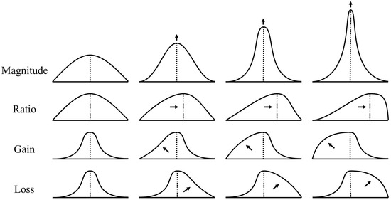
Figure 1.
Change in latent variable values for each geometric characteristic. In a left-to-right order, the arrows represent the increase in the geometric characteristic: Magnitude, Ratio, Gain, and Loss.
Since the output of the encoder is , one can use any norm over for the peak series distance function . Each geometric characteristic can be emphasized by its importance to the contribution to the value of the norm, and, therefore, change the meaning of the distance between different peaks.
3.2.3. Unit-Less Encoding
We introduce a unit-less encoding that combines the characteristics of the peak graph encoder as follows:
The four values of the encoding are between 0 and 1, , ensuring that the proposed encoder is unit-less. This encoding will be used for further analysis of the discrete case in the following section.
3.3. Discrete Case
The discrete case is crucial to real-world signal recordings. MEG data consist of time series which are recordings of the MEG sensors (channels) sampling. However, the definitions and constructions in this section are relevant to any discrete case, and therefore a discrete method is given as well.
3.3.1. Peak Series
Peak Series S is a sampling of a peak graph image S:= that satisfies the following conditions:
The set of all series, of length N, following those conditions, is called the Set of Peak Series of length N and denoted as .
3.3.2. Encoding of a Peak Series
As mentioned in Section 3.1.3, a series operator can be defined directly using the naive discrete calculation for each one of the four coordinates of the latent space.
The encoder encodes a peak series of length N as follows:
3.3.3. Equivalence Relation on
We define the equivalence relation on via the encoder from Equation (1). Let be two peak series of length N:
We denote by the equivalence class of under :
In terms of the equivalence relation , the quotient space is the set of equivalence classes over the equivalence relation:
3.3.4. Distance Function on the Discrete Quotient Space
We construct a distance function on by
where is the standard norm on .
Note: we can replace the standard norm used in the definition of the distance function d by a norm on to obtain .
Note: , a generalization of the distance function for the equivalence classes of different length peak series, can be defined as follows:
when the lengths of the series respectively, are not necessarily equal.
3.3.5. Normalization
We say that the sampling rate of a peak series S of length is the number of values measured in a time interval of one second (Hz).
In terms of peak series, a sampling rate coupled with the whole number of samples in the series can provide an approximation for the duration of the recording, noted as
when the sampling rate indicates how dense is the recording, and D is the real length (in time units) of sampling.
The motivation for the following definition is to provide a uniform time-scale encoding for various sampling rates’ peak series.
We define the normalization encoder of a peak series S of length N coupled with a sampling rate of as follows:
Let be two peak series coupled with sampling rates of respectively. The normalized distance function for is identical to the one defined in Section 3.3.4:
3.3.6. Cube Encoding
To provide a partition to the set of peak series, we introduce a discrete encoding, combining the geometric characteristics in a binary 4-dimensional form, hence named Cube Encoding.
Let S be a peak series of length N and with a sampling rate of . For convenience, we denote the terms of as follows:
We define the Cube Encoding of a Peak Series of length N and sampling rate as follows:
The thresholds for each of the terms were chosen directly following the unit-less encoding (Section 3.2.3), such that the values of the thresholds will correspond to (a half) on each of the terms of the continuous unit-less encoding.
Note that , is a point on the 4-dimensional unit cube, and has 16 possibilities. This finite structure will be useful for early estimation and sorting of the peak series extracted from real MEG recordings.
3.4. The Algorithms
Based on the definitions and constructions in Section 3.2 and Section 3.3, we obtain two algorithms that are related to the discrete case of the digitized signal of a peak that we defined before as the peak series.
3.4.1. Algorithm 1: Encoder for a Peak Series
Algorithm 1 corresponds to the operation of the encoder, from Equation (1) (Section 3.3.2), over a peak series. The input is a vector of length N and an integer, and the output is a 4-length vector. It has a run-time complexity of when N is the length of the input vector. Note that both Gain and Loss are evaluated with the value at the peak.
| Algorithm 1 Encoder for peak series of length N |
|
3.4.2. Algorithm 2: Scaled Sampling Rate Distance Function
Algorithm 2 corresponds to the operation of the normalized distance function, from Equation (2) (Section 3.3.5), over two peak series coupled with sampling rates. The inputs are a vector of length N, a vector of length K, and two integers, and the output is a real (non-negative) number. It has a run-time complexity of when N and K are the same lengths of the input vectors.
| Algorithm 2 Distance function for peak series of lengths and sampling rates |
|
3.5. Implementation of the Algorithms
Working with peak series is intuitive as long as we can assure that they are indeed peak series, elements of . Before applying the algorithms, we need to validate that we have a peak series. There are many validations that at least return a sub-series of the original one taken from a single channel, which is a peak series. One can use the numpy.ndarray (Numpy, 2022) [9] and pandas.DataFrame (Pandas, 2023) [10] modules (versions numpy==1.26.4, pandas==2.0.3), that contain a lot of tools that can help in tabular manipulation in order to extract a required sub-series which is a peak. For example, one can choose a specific channel from the matrix of channels (Table 1) and take any sub-series of it. Furthermore, one can use transformations such as the Principal Component Analysis over a set of channels in order to create a new time series representing multiple sensors together.
A very popular tool for the validation of a peak series, implemented in Python, is the find_peaks() (https://docs.scipy.org/doc/scipy/reference/generated/scipy.signal.find_peaks.html (accessed on 12 October 2025)) program function (SciPY, 2021) [11] which has a lot of parameters controlling the height, width, and more properties of the extracted peak (version scipy==1.14.1).
The algorithms assume a single distinct maximum for a peak series (corresponding to the definition). However, real data may have multiple maximum points. In our case, the first maximum is taken. Moreover, non-peak time series are omitted and will not be considered as peak series for later analysis.
After validation that some series S of length N is a peak series, one can apply Algorithm 1 to encode S via . As for Algorithm 2, once the encoding of the compared peak series is completed, one can apply the distance function directly, only for a run time complexity of (for each pair of series).
In most cases, actual data recordings are not of the same length and may have different sampling rates. That is why we use the more general distance function for different lengths and/or sampling rates peak series as defined in Section 3.3.5. An implementation in Python for relatively popular and standard norms, as shown at the end of Algorithm 2, can be found in the numpy.linalg.norm (https://numpy.org/doc/stable/reference/generated/numpy.linalg.norm.html (accessed on 12 October 2025)) (version numpy==1.26.4) module (Numpy, 2022) [9].
4. Results
The distance function that we built is very strong in order to measure the similarity or distance between the original sources of digital recording. For the evaluation of our distance function (Section 3.1.5) in comparison to the other methods mentioned in Section 1.1.2, we used specific analytic peak graphs, over the section . We also evaluated over peak series extracted from MEG recordings.
4.1. Evaluation over Analytic Peak Graphs
In order to evaluate our distance function in a compartment with the and DTW (Dynamic Time Warping) over peak graphs, we have built each analytic real function corresponding to a specific geometric characteristic. For each characteristic, we chose three functions having three different values for such characteristics, while approximately the same value for the others. For example, for the Magnitude property, we have explicitly defined peak graphs having different Magnitudes at the peak (extreme point) while preserving the values of the Ratio, Gain, and Loss constant (as shown in Figure 2). Notice that the Loss is equivalent to the Gain, and therefore not included (for symmetry considerations).
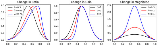
Figure 2.
Different latent variable values for each geometric characteristic in peak graphs. The graphs in the change in Ratio are , in the change in Gain are , and in the change in Magnitude are .
- Magnitude—An approximation of the famous Dirac’s Delta function has been defined (Zahedi, 2010) [12] and shifted correctly to the peak graph definition in Section 3.1.1 in order to achieveis a peak graph by definition, and its magnitude is controlled by the parameter . Notice that because , we shifted the approximation slightly by subtracting its value on the edges , and therefore we obtain the desired result of the peak graph .For h small enough, we obtain that the Gain and Loss of are half of , that is, of course, , and having a constant Ratio 1.For Magnitude, we chose the values of h to be , and measured the ratio:
- Ratio—Similarly to example 3 in Section 3.2.1, we constructed a peak graph that can be controlled in terms of the Ratio, Gain, and Loss only:Notice that the Magnitude is constant and equals for any . It is simple to show that is constant:Note ; hence, we obtain thatwhich is constant. However, the Gain is now and the Loss is now .For Ratio, we chose the values of to be , and measured the ratio:
- Gain—The Gain (or Loss) of any peak graph, of Magnitude equal to 1, can be easily controlled by raising its Gain (or Loss) part to the power of . We can achieve such a peak graph by taking from Equation (4) and normalizing it by dividing it by the value of Magnitude. Hence, we define it byFor Gain, we chose the values of p to be , and measured the ratio:
For the evaluation of each of the distance functions’ sensitivity to the change in Magnitude, Ratio, and Gain, separately, we measured the ratio of the distance (value of the distance function) between two relatively close (in geometric terms) peak graphs, and two slightly more distant peak graphs.
The sampling resolution for each peak graph was 100 uniformly distributed points. And finally, we obtain the results , calculated via each of the distance functions—DTW, , and our distance function, in Table 2.
Table 2.
The ratio between the distances of close and distant peak graphs depends on the choice of the distance function. Lower values indicate better sensitivity.
While our distance function is in second and third places for changes in Magnitude and Gain, respectively, it is best for measuring the change in Ratio, which corresponds to the asymmetry of the peaks. Moreover, the change in the Ratio, in this test, combines a change in Gain and Loss as well. Unlike the isolated changes in Magnitude and Gain. Therefore, the overall distance between shifts in the peak graphs is more sensitive to our distance function.
The analytical peak graphs for each category of change in geometric characteristic are presented in Figure 2.
4.2. Evaluation over Noisy Analytic Peak Graphs
For the simulation of real data recordings, we added noise to the nine peak graphs we chose in Section 4.1 (three peak graphs for each one of the three characteristics—Magnitude, Ratio, and Gain). A random noise of the normal distribution was generated with a seed and added to the value of each peak graph at every sampling point. We repeated this process 10 times, each with a unique constant seed.
The results for the ratios , , , calculated over the noisy peak graphs , , (whose graphs can be seen in Figure 3), respectively, are presented in Table 3 as mean values and their standard deviations over all 10 repetitions.
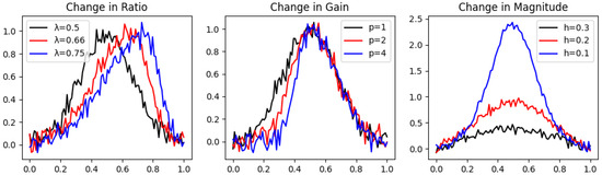
Figure 3.
Different latent variable values for each geometric characteristic in noisy peak graphs. The graphs in the change in Ratio are , in the change in Gain are , and in the change in Magnitude are .
Table 3.
The ratio between the distances of close and distant noisy peak graphs depends on the choice of the distance function. Lower values indicate better sensitivity.
Our distance function leads in both . However, since measures the integral of the square of the function, its is more affected by added random noise, leading in second place. SBD remains in first place, unaffected drastically by the added noise in terms of the change in Gain; however, it loses its advantage in terms of the change in magnitude when noise is added.
These synthetic test cases (Section 4.1 and Section 4.2) simulate real data by considering natural artifacts of peak/spike moments in MEG time series. These tests provided a baseline to elaborate and evaluate our distance function over MEG recordings.
4.3. Evaluation over Different Projections of MEG Recordings
We tested real data recordings taken from a session of a subject’s brain activity. We extracted 10-time series from 10 different channels of the MEG device, a couple from distant areas of the scalp, during a peak. Denote as the recording from area and channel during that peak. Notice that c does not represent the actual MEG sensor number; rather it is the index of a specific sensor from some area a. The recordings of that peak are presented in Figure 4.
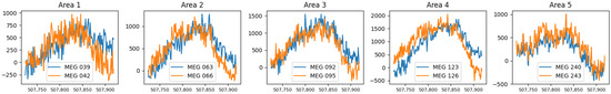
Figure 4.
Five couples of projections, of the MEG recordings during peak time, sampled in close channels (MEG sensors) from five different areas of the scalp.
For the comparison of our distance function to DTW and , we measured the average ratio of the distance between peak series from the same area to each distance between cross-area peak series , using distance function d, in the following way:
when are the two different channels 1, 2, respectively, and from the outer sum are not the same area.
The graph of the value of at area is presented in Figure 5. Table 4 concludes the results by showing the average value of for all areas .
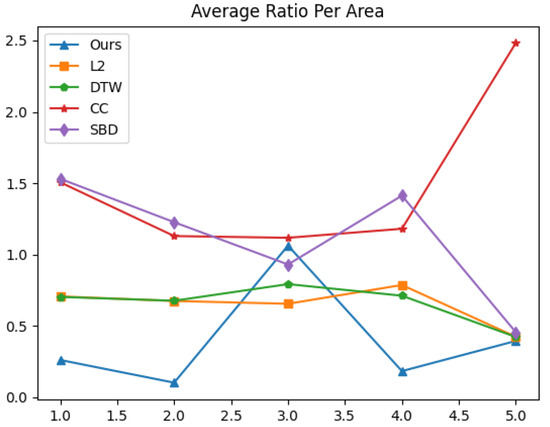
Figure 5.
Average ratio of close sampled peaks’ distance to distant (cross area) peaks’ distance per area, for each distance function.
Table 4.
Value of per area (lowest is better) for each distance function.
The higher average ratio per area 3 presented in Table 4, performed by our distance function, may be connected to a mislabeling of a hidden local minimum in the last quarter of the time series of channel MEG 095. Since we show real data performances, we forbid any manipulations of the data (smoothing/filtering).
Overall results show a significant advantage of our distance function, indicating higher sensitivity to the spatial resolution of the brain activity in general, and the peak source specifically. This fact encourages us to have a more robust evaluation of our method over spatially clustered MEG extracted peaks.
4.4. Evaluation over Local Neighboring MEG Sensors Categorized by Cube Encoding
We tested real data recordings taken from a subject’s brain activity full session. We used find_peaks(signal, width=(30, 120), rel_height=1, distance=120) (Section 3.5), to detect and extract non-overlapping peak segments within each of the 248 sensors recording, having a width of approximately 30 to 120 ms, above zero amplitude. This configuration relates to a parametric description of MEG peaks measured and extracted simultaneously with depth electrode spikes (Rafal Nowak and Marta Santiuste and Antonio Russi, 2009) [13].
To address spatially clustered peaks by their morphology, we calculated the cube encoding of all extracted peak series. Then, for each vertex of the 4-dimensional cube (), if there are peaks encoded to that vertex, we picked the peak series of the sensor with the most peaks of that vertex, with its neighboring sensors’ peak series, according to the sensors’ adjacency map (using find_ch_adjacency() from mne.channels module) presented in Figure 6.
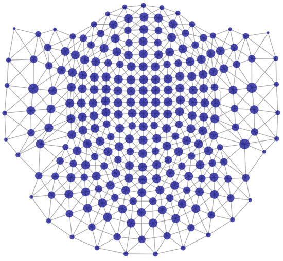
Figure 6.
Sensors’ adjacency map of the 4D-BTi MEG device. The nodes are the sensors, and the links represent adjacency. The size of the nodes corresponds to the number of neighboring sensors—bigger nodes have more neighbors.
We calculated the distances between all pairs of peak series of the leading sensor (denoted by ) and the distances between all pairs of peak series with one peak from the leading sensor and the second from a neighbor sensor (denoted by ). Hence, we demand at least two peaks from the leading sensor, and one peak for each neighbor. Otherwise, they were removed from calculations.
We measured the values of using our distance function (Section 3.3.4) and the existing appropriate methods ( and cross-correlations are incompatible with different lengths of peak series and therefore omitted). The results are presented in Table 5.
Table 5.
The ratio between the average value of and the average value of , calculated for each cube encoding via existing methods and ours. The number of neighboring sensors (#Neighbors), the number of inner sensor peaks (#in-peaks), and the number of outer sensor peaks (#out-peaks) are provided with each cube encoding evaluation. Lower values indicate better sensitivity to local peak sorting.
The results show a consistent lead of our distance function in terms of high-resolution peak sorting and similarity by different peak morphologies (cube encoding) over raw MEG recordings.
5. Discussion
From the final results of both analytic peak graphs (pure or noisy) and peak series of real MEG recordings, one can conclude that our distance function is the most precise one in terms of geometric properties’ measurement (relates to both time and space dimensions simultaneously). More so, it enables the control of the specific geometric characteristic only by changing the standard norm.
Our research shows a few—simple yet efficient—applications of the encoding and distance function we have defined with minimal to no pre-processing of raw data. In future research, it will serve as a foundation for basic signal analysis. Note that this is the first ever geometric characteristic encoder and distance function for peak graphs.
Moreover, the peak sorting technique we showed can be applied in the medical field and provide a high accuracy for a non-invasive detection and spatial-temporal clustering of spike events like epilepsy seizures.
Author Contributions
Conceptualization, A.K. and M.T.; methodology, A.K.; software, A.K.; validation, A.K. and M.T.; formal analysis, A.K.; investigation, A.K.; resources, A.K.; data curation, A.K.; writing—original draft preparation, A.K.; writing—review and editing, A.K. and M.T.; visualization, A.K.; supervision, M.T.; project administration, M.T.; funding acquisition, M.T. All authors have read and agreed to the published version of the manuscript.
Funding
No funding was received for conducting this study. The authors have no relevant financial or non-financial interests to disclose.
Data Availability Statement
No new data were created or analyzed in this study. Data sharing is not applicable to this article.
Conflicts of Interest
The authors declare no conflicts of interest.
References
- Peixeiro, M. The Complete Guide to Time Series Analysis and Forecasting. 2019. Available online: https://medium.com/the-forecaster/the-complete-guide-to-time-series-analysis-and-forecasting-70d476bfe775 (accessed on 11 October 2025).
- Müller, M. Dynamic Time Warping; Springer: Berlin/Heidelberg, Germany, 2007; pp. 69–84. [Google Scholar]
- Paparrizos, J.; Gravano, L. Fast and Accurate Time-Series Clustering. In ACM Transactions on Database Systems; ACM: New York, NY, USA, 2017; Volume 42, pp. 1–49. [Google Scholar]
- Hämäläinen, M.; Hari, R.; Ilmoniemi, R.J.; Knuutila, J.; Lounasmaa, O.V. Magnetoencephalography—Theory, instrumentation, and applications to noninvasive studies of the working human brain. Rev. Mod. Phys. 1993, 65, 413–497. [Google Scholar] [CrossRef]
- Cohen, D.; Cuffin, B.N. Demonstration of useful differences between magnetoencephalogram and electroencephalogram. Electroencephalogr. Clin. Neurophysiol. 1983, 56, 38–51. [Google Scholar] [CrossRef] [PubMed]
- Okamura, A.; Iida, K.; Hashizume, A.; Kagawa, K.; Seyama, G.; Horie, N. Magnetoencephalographic spikes with small spikes on simultaneous electroencephalography have high spatial clustering in temporal lobe epilepsy. Epilepsy Res. 2023, 192, 107–127. [Google Scholar] [CrossRef] [PubMed]
- FieldTrip Toolbox. Getting Started with Bti/4D Data. 2021. Available online: https://www.fieldtriptoolbox.org/getting_started/bti (accessed on 12 October 2025).
- Gramfort, A.; Luessi, M.; Larson, E.; Engemann, D.A.; Strohmeier, D.; Brodbeck, C.; Goj, R.; Jas, M.; Brooks, T.; Parkkonen, L.; et al. MNE. Reading Raw Data, (Version==1.8.0). 2021. Available online: https://mne.tools/stable/generated/mne.io.read_raw_bti.html?highlight=rawbti (accessed on 12 October 2025).
- Harris, C.R.; Millman, K.J.; van der Walt, S.J. Numpy. Numpy.Ndarray, (Version==1.26.4). 2022. Available online: https://numpy.org/doc/stable/reference/generated/numpy.ndarray.html (accessed on 12 October 2025).
- Pandas. Pandas.Dataframe, (Version==2.0.3). 2023. Available online: https://pandas.pydata.org/docs/reference/api/pandas.DataFrame.html (accessed on 12 October 2025).
- Virtanen, P.; Gommers, R.; Oliphant, T.E.; Haberland, M.; Reddy, T.; Cournapeau, D.; Burovski, E.; Peterson, P.; Weckesser, W.; Bright, J.; et al. SciPY. Signal Processing. 2021. Available online: https://docs.scipy.org/doc/scipy/reference/generated/scipy.signal.find_peaks.html (accessed on 12 October 2025).
- Zahedi, S. Delta function approximations in level set methods by distance function extension. J. Comput. Phys. 2010, 229, 2199–2219. [Google Scholar] [CrossRef]
- Nowak, R.; Santiuste, M.; Russi, A. Toward a definition of MEG spike: Parametric description of spikes recorded simultaneously by MEG and depth electrodes. Seizure 2009, 18, 652–655. [Google Scholar] [CrossRef] [PubMed]


Disclaimer/Publisher’s Note: The statements, opinions and data contained in all publications are solely those of the individual author(s) and contributor(s) and not of MDPI and/or the editor(s). MDPI and/or the editor(s) disclaim responsibility for any injury to people or property resulting from any ideas, methods, instructions or products referred to in the content. |
© 2025 by the authors. Licensee MDPI, Basel, Switzerland. This article is an open access article distributed under the terms and conditions of the Creative Commons Attribution (CC BY) license (https://creativecommons.org/licenses/by/4.0/).