Article

A Clustered Link-Prediction SEIRS Model with Temporal Node Activation for Modeling Computer Virus Propagation in Urban Communication Systems

1
School of Mechanical Engineering, Tongji University, Shanghai 200092, China
2
School of Economics and Management, Tongji University, Shanghai 200092, China
3
College of Civil Engineering, Guizhou University, Guiyang 550025, China
*
Author to whom correspondence should be addressed.
AppliedMath 2025, 5(4), 128; https://doi.org/10.3390/appliedmath5040128
Submission received: 6 August 2025 / Revised: 29 August 2025 / Accepted: 19 September 2025 / Published: 25 September 2025

Abstract

We propose the Clustered Link-Prediction SEIRS model with Temporal Node Activation (CLP-SEIRS-T), a novel epidemiological framework that integrates community structure, link prediction, and temporal activation schedules to simulate malware propagation in urban communication networks. Unlike traditional static or homogeneous models, our approach captures the heterogeneous community structure of the network (modular connectivity), along with evolving connectivity (emergent links) and periodic device-usage patterns (online/offline cycles), providing a more realistic portrayal of how computer viruses spread. Simulation results demonstrate that strong community modularity and intermittent connectivity significantly slow and localize outbreaks. For instance, when devices operate on staggered duty cycles (asynchronous online schedules), malware transmission is fragmented into multiple smaller waves with lower peaks, often confining infections to isolated communities. In contrast, near-continuous and synchronized connectivity produces rapid, widespread contagion akin to classic epidemic models, overcoming community boundaries and infecting the majority of nodes in a single wave. Furthermore, by incorporating a common-neighbor link-prediction mechanism, CLP-SEIRS-T accounts for future connections that can bridge otherwise disconnected clusters. This inclusion significantly increases the reach and persistence of malware spread, suggesting that ignoring evolving network topology may underestimate outbreak risk. Our findings underscore the importance of considering temporal usage patterns and network evolution in malware epidemiology. The proposed model not only elucidates how timing and community structure can flatten or exacerbate infection curves, but also offers practical insights for enhancing the resilience of urban communication networks—such as staggering device online schedules, limiting inter-community links, and anticipating new connections—to better contain fast-spreading cyber threats.

1. Introduction

Urban communication networks—comprising the interlinked computer systems, IoT devices, and infrastructure that enable city-wide connectivity—form the backbone of modern smart cities. Ensuring the resilience of these networks against disruptions is paramount, as failures can cascade into broader socio-economic impacts. One critical threat to network resilience is the rapid propagation of computer viruses and malware, which can spread autonomously through communication links analogously to contagious diseases. Recent cyberattacks have underscored the destructive potential of self-propagating malware: for instance, the 2017 WannaCry ransomware outbreak infected over 200,000 computers across more than 150 countries within days, causing hundreds of millions of dollars in damages [1]. Likewise, the 2021 Colonial Pipeline incident demonstrated that malware-induced network outages can even disrupt critical urban infrastructure services [2]. In another example, the Mirai botnet in 2016 hijacked over a million Internet-of-Things (IoT) devices to launch massive distributed denial-of-service (DDoS) attacks, temporarily knocking major online services offline [3]. These incidents illustrate that computer virus epidemics in urban communication systems can spread with alarming speed and scale if not adequately contained. This motivates a pressing need for advanced modeling frameworks to understand and mitigate malware propagation in complex networked environments.
However, existing models often neglect the temporal dynamics and evolving topology of networks. In fact, recent studies in other domains have begun to address complex spatiotemporal dynamics using data-driven methods. For example, Zhang et al. developed a Koopman mode decomposition approach to model spatial–temporal correlations in sea clutter [4], Ding et al. proposed a time-varying channel model for UAV air–ground communication [5], Zhang and Jiang applied dynamic mode decomposition to analyze electromagnetic radiation patterns [6], and a data-driven scheme was introduced for identifying ship wakes on dynamic sea surfaces [7]. Inspired by the success of these approaches in capturing temporal complexities, this paper introduces the CLP-SEIRS-T model—a novel extension.
Classical epidemic models from mathematical epidemiology provide a natural starting point for modeling computer virus spread. Traditional compartmental models such as SIR (Susceptible–Infectious–Recovered) and SIS (Susceptible–Infectious–Susceptible) were originally developed to capture infectious disease dynamics in well-mixed populations [8]. In these models, individuals (or nodes) are classified into discrete states and transition between states according to infection or recovery rates. The SIR model, for example, assumes that infected nodes eventually recover with immunity, whereas the SIS model assumes no lasting immunity, allowing recovered nodes to become susceptible again. Another important extension is the SEIR model, which introduces an Exposed (latent) compartment to represent an incubation period during which individuals are infected but not yet infectious. The SEIRS variant further allows recovered individuals to lose immunity and return to the susceptible state after some time [9]. These epidemiological frameworks have been widely applied to study malware propagation by drawing an analogy between biological contagion and computer infections [10,11]. In the context of computer viruses, the “susceptible” state corresponds to vulnerable devices, the “infectious” state corresponds to actively compromised devices spreading the malware, and a “recovered” node is a device that has been disinfected or patched [12]. An Exposed state can represent infected devices that are not yet actively spreading (for example, malware that has infiltrated a system but remains dormant until a trigger). Temporary immunity in recovered devices may correspond to short-term protection (e.g., through patches or security updates) that can wane as new vulnerabilities emerge, making the device susceptible again.
Building on these foundations, a variety of extended compartmental models have been proposed to better capture the nuances of computer malware outbreaks. For instance, some models include the impact of external infection vectors such as removable media or peer-to-peer file sharing on virus spread [13], or incorporate resource limitations and user intervention effects [14]. Others introduce additional states to represent malware-specific phenomena (e.g., an “alert” or dormant infected state, or multiple infection stages) [15,16]. These enriched models provide deeper insight into malware dynamics, and their theoretical behavior has been analyzed using mean-field techniques [17]. However, the majority of prior works in this vein assume homogeneous mixing or highly simplified network structures, and often lack validation on realistic network data [18]. This highlights the need for models that explicitly account for network topology and time-varying connectivity when examining computer virus propagation.
Over the past two decades, a significant body of research in network science has shown that the topology of connections plays a decisive role in contagion dynamics [19,20]. Structural heterogeneities in complex networks can dramatically affect virus propagation [21]. In particular, networks with heavy-tailed degree distributions (such as scale-free networks) are highly vulnerable to epidemics: even malware with low infectivity can persist and reach a large fraction of nodes because hubs with many connections greatly amplify the spread [22]. The epidemic threshold—the critical infection rate above which a virus outbreak becomes global—tends to be substantially lower (approaching zero in infinite scale-free networks) than predicted by classic well-mixed models [23]. This fragility of heterogeneous networks to malware spread has been demonstrated in numerous studies [24], highlighting that network structure is a crucial factor in assessing cyber-epidemic risk. Moreover, graph-based epidemic models (which map hosts to nodes and communication links to edges) enable the use of network metrics and spectral analysis to predict outbreak conditions and sizes [25,26]. For example, the largest eigenvalue of a network’s adjacency matrix is directly related to the epidemic threshold in SIS-type models [27]. These insights underscore that any realistic computer virus propagation model must explicitly account for the underlying network topology rather than assuming random mixing.
Beyond degree heterogeneity, clustered or modular structure is another salient feature of real urban communication networks that can influence epidemic dynamics [28]. Communication networks often exhibit community structure, wherein nodes form tightly knit groups (clusters) with dense intra-group connections but relatively sparser inter-group links. Examples include subnetworks corresponding to departmental LANs within an enterprise, or neighborhoods of IoT devices that predominantly communicate locally. Such modular organization can either impede or accelerate the spread of malware, depending on the interplay between intra- and inter-community transmissions [29]. On one hand, strong community boundaries can act as firebreaks that localize infections: a virus may saturate one cluster but struggle to jump to others if inter-community links are limited. This effect tends to slow down SIR-type outbreaks and reduce their final reach by confining the epidemic within communities. On the other hand, in SIS-type scenarios (or persistent malware that can repeatedly reinfect nodes), community structure can sometimes facilitate the epidemic by allowing the pathogen to persist in isolated clusters and periodically re-emerge, effectively lowering the overall epidemic threshold compared to an equivalent random network without communities. The contrasting effects observed in recent studies indicate that network modularity introduces non-trivial dynamics highly relevant for computer virus propagation. However, most classical epidemic models for malware do not explicitly incorporate community structure, instead treating the network as either fully mixed or as an unstructured graph. Incorporating clustered connectivity into propagation models is essential for accurately capturing the resilience or vulnerability of segmented real-world networks. Additionally, epidemic processes have also been studied in interconnected multilayer networks (e.g., concurrent spread of malware and information), offering insight into cross-layer effects [30]. In this work, however, we focus on a single-layer network model.
Another key aspect of urban communication networks is their time-varying nature. The connectivity between devices is not static: links can appear, disappear, or change over time due to mobility, device duty cycles, usage patterns, and other factors [31]. For example, smartphones and laptops connect to different Wi-Fi access points throughout the day, industrial control systems may reconfigure network links at scheduled intervals, and IoT sensors often activate and deactivate periodically to conserve energy. Traditional static network models approximate a constantly connected topology, which fails to reflect these temporal fluctuations. Recent research on epidemics in temporal networks shows that temporal structure can substantially alter infection dynamics compared to static graphs [32]. Temporal contact patterns (especially those that are bursty or periodic) may slow down the spread of infections by reducing the overlap of infectious periods with contact, or conversely, may synchronize with virus dynamics to create bursts of transmission [33]. For instance, if interactions are concentrated in short, intense bursts separated by longer inactive periods, an infected node might recover before it has a chance to pass the virus during the next burst, thereby lowering transmissibility relative to a time-aggregated view [34]. Conversely, certain temporal patterns can amplify spreading; an illustrative case is when daily or weekly behavioral cycles resonate with the latent or infectious period of the malware, leading to a higher reach of the contagion [35]. Therefore, capturing the timing and ordering of contacts is crucial for modeling malware spread in real networks. Approaches like activity-driven networks have been proposed to generate synthetic time-varying contact graphs, where nodes have intrinsic activity rates dictating the creation of links over time [36]. These models reproduce realistic temporal phenomena (e.g., heterogeneous inter-contact times and circadian cycles) and have been used to study epidemic processes on evolving networks. Asynchronous periodic node behavior is a particularly important temporal pattern in urban networks: different nodes may exhibit periodic connectivity cycles (daily or weekly routines) that are not synchronized with each other [37]. For example, consider a set of enterprise networks that are active during workdays and largely offline overnight, versus home networks that are more active on evenings and weekends. If a malware’s infectious period overlaps with the active hours of one cluster but falls during the quiescent hours of another, propagation can be impeded by this lack of temporal alignment. In some cases, alternating connectivity schedules can even produce counter-intuitive outcomes, such as a virus dying out on an alternately switching two-network system even if it would persist on each network individually, a phenomenon recently termed a “Parrondo paradox” in epidemic dynamics. These findings stress that models for computer virus spread must move beyond static graphs and homogeneous time assumptions to incorporate the temporal (and often periodic) nature of network links and node activity patterns.
In addition to structural and temporal complexities, an emerging consideration is the partial observability and unpredictability of network evolution. In practical scenarios, one may not have complete knowledge of all connections in a large urban communication network, and new links (for instance, new devices coming online or previously disconnected sub-networks becoming interconnected) can arise over time. Link-prediction techniques from network science offer a way to anticipate likely future or missing connections based on observed network patterns [38]. By leveraging features such as shared neighbors, communication frequencies, or community membership, link-prediction algorithms estimate the probability that a pair of nodes will form a link in the near future [39]. Integrating link prediction into epidemic modeling can enhance realism by accounting for the fact that malware might exploit not only present connections but also potential connections that are likely to materialize as the network evolves. For example, if two currently separate network clusters have a history of intermittent data exchange, a predictive model might foresee a high likelihood of future contact between them, which a virus could eventually exploit. Proactively modeling such prospective links could improve forecasts of malware reach and help identify critical “bridging” links to secure preemptively [40]. Notably, prior studies on adaptive networks have considered scenarios where contacts change in response to the epidemic (e.g., susceptible nodes rewiring or cutting links to avoid infection) [41,42]. However, those models focus on behavioral adaptation of the network, rather than anticipating intrinsic network growth or reconnection. Incorporating a link-prediction mechanism is a novel approach that allows an epidemic model to account for network topology changes independent of the virus dynamics. To date, most epidemic propagation models do not dynamically integrate link prediction; they either assume a fixed network or allow random link churn without leveraging predictive insights. This represents a clear gap in our ability to model malware spread on emerging and evolving communication infrastructures.
Summarizing the above, we identify several research gaps that motivate the development of an enhanced modeling framework for computer virus propagation. First, there is a need to unify clustered network structure with time-varying connectivity in a single model. Previous studies have largely examined community effects and temporal dynamics separately, and only a few works have begun to explore their combined impact. The interplay between modular topology and temporal link patterns in spreading processes remains not fully understood, especially in the context of cyber-epidemics on city-scale networks. Second, existing malware epidemic models often assume synchronous contacts or neglect the periodic and asynchronous activation patterns observed in real networks. Such simplifications may lead to inaccurate predictions of outbreak timing and size. Third, conventional models usually consider a known, static topology, failing to account for emerging links and the uncertain evolution of the communication graph over time. This limits their applicability to dynamic urban networks where connectivity changes and new interactions can open unforeseen infection pathways.
To address these gaps, this paper introduces the CLP-SEIRS-T model—a novel extension of the classical SEIRS epidemic model that incorporates Clustered structure (C), Link Prediction (LP), and Temporal node activation (T). In our CLP-SEIRS-T framework, the population of devices is partitioned into clusters (communities) to reflect modular network organization, and virus transmission is modeled both within and between these clusters. A link-prediction module is integrated to foresee likely future connections or re-activation of dormant links, thereby dynamically adjusting the contact network as the epidemic unfolds. Additionally, each node is endowed with an asynchronous periodic activation schedule, meaning that nodes switch between active (online) and inactive (offline) states in a repeating pattern, but not all nodes share the same phase or period. This feature captures the staggered usage cycles of devices in an urban setting (for example, devices in different time zones or on different work shifts). The CLP-SEIRS-T model thus simulates malware propagation on a time-varying network that evolves according to both predictable routines and stochastic link formations, offering a more faithful representation of urban communication ecosystems. In doing so, our approach builds upon and extends recent epidemiological models for malware—for example, individual-based SEIRS models for IoT environments [43] and new compartmental formulations like the SIIDR model—by explicitly incorporating network clustering and temporal dynamics within a unified framework. In contrast to previous temporal SEIRS models which include time-varying contacts but often assume homogeneous or synchronized activity patterns, our CLP-SEIRS-T model introduces asynchronous, node-specific activation cycles and a link-prediction module on top of a community-structured network. To our knowledge, this is the first malware propagation model that combines community modularity, evolving predicted connectivity, and asynchronous temporal dynamics in one framework. Earlier works have typically considered only one or two of these aspects separately. For example, some activity-driven SEIR models capture temporal contact fluctuations but ignore underlying community structure [44,45,46], while existing adaptive network models allow link rewiring in response to infection but do not predict new links. By integrating all these features, our approach provides a novel and more comprehensive perspective.
The purpose of this study is to formula a model that provides a comprehensive platform for the examination of computer virus propagation from a complex-network perspective, wherein structural, temporal, and predictive components are integrated. Through the application of the CLP-SEIRS-T framework, the combined effects of community modularity and inferred connectivity on malware propagation speed and overall reach are analyzed, and the influence of periodic node activation on epidemic thresholds and persistence is elucidated.

2. Model Formulation

The CLP-SEIRS-T model is a compartmental network model that extends a standard SEIRS epidemic framework by incorporating Common-neighbor Link-Prediction (CLP) mechanisms and time-periodic contact activation for each node. This section presents the model’s structure, parameters, and mathematical derivations, including the state transition equations and differences from the original CLP-SEIRS model [47]. We assume throughout that the contact network is a simple undirected, unweighted graph. Key model parameters and variables are summarized in Table 1 for reference.

2.1. Model Setup and State Definitions

We consider a network of N individuals (nodes) whose virus states evolve according to an SEIRS compartmental model:
Susceptible Exposed Infectious Recovered Susceptible .
In this model, each node i at time t can be in one of four possible states:
  • Susceptible   S i ( t ) : Node i is healthy and vulnerable to infection.
  • Exposed   E i ( t ) : Node i has been infected but is not yet infectious (latent period).
  • Infectious   I i ( t ) : Node i is actively infected and can transmit the virus to susceptible neighbors.
  • Recovered   R i ( t ) : Node i has recovered and is temporarily immune (will later lose immunity and return to susceptible).
These state variables can be treated as indicator functions (e.g., S i ( t ) = 1 if node i is susceptible at time t, else 0, etc.), or equivalently as probabilities in a mean-field sense. Similarly for E i ( t ) , I i ( t ) , and R i ( t ) . At any time, exactly one of S i , E i , I i , R i , is 1 for each node i and the others 0, implying
S i ( t ) + E i ( t ) + I i ( t ) + R i ( t ) = 1 for all i = 1 , , N .

2.2. Contact Network and Link-Prediction Mechanism

Nodes interact according to a contact network represented by an adjacency matrix A = [ A i j ] of size N × N . Here, A i j = 1 if there is a direct contact edge between nodes i and j, and A i j = 0 otherwise. We assume an undirected network, so A i j = A j i , and no self-loops A i i = 0 . An edge A i j = 1 indicates that if either i or j is infectious, it can potentially expose the other upon contact.
Community structure: We assume the network is divided into communities (or groups) such that each node i belonging to a community C i . The model accounts for stronger ties (higher infection rates) within communities and weaker ties across communities. Let:
  • β : infection rate for an infectious contact within the same community (intra-community transmission rate),
  • ρ : infection rate for an infectious contact across different communities (inter-community transmission rate).
Define the pairwise infection rate β i j to denote the infection rate applicable between node i and j:
β i j = β , if C i = C j ( same community ) , ρ , if C i C j ( different communities ) .
Typically, we expect ρ < β , reflecting that cross-community contacts transmit virus at a lower rate than within-community contacts.
Link-prediction mechanism (common neighbors): In addition to static direct links, the CLP-SEIRS-T model features a mechanism for dynamic contact formation based on link prediction. Specifically, even if two nodes are not directly connected in A, they may still come into contact through mutual acquaintances (common neighbors). If node i and node j share one or more common neighbors in the network, those mutual connections can facilitate an introduction or meeting between i and j. We model this effect by assigning an indirect infection rate λ per common neighbor. In other words, for each distinct node k that is connected to both i and j ( A i k = 1 and A k j = 1 ), there is a potential infection pathway linking i and j at rate λ . This models the idea that mutual friends or network structure can predict new contacts (hence “link prediction”).
Let C i j denote the number of common neighbors between i and j:
C i j = k = 1 N A i k A k j ,
which counts all nodes k that simultaneously neighbor both i and j. If C i j > 0 (meaning i and j have at least one mutual neighbor), then i and j can form an effective contact even if A i j = 0 . We assume each common neighbor contributes additively to the contact rate, so that the total predicted contact rate between i and j (if not directly connected) is λ C i j . In summary:
  • A direct link A i j = 1 uses rate β i j (either β or ρ depending on community relation).
  • An indirect connection through common neighbors ( A i j = 0 and C i j > 0 ) uses rate λ C i j .
We emphasize that these common-neighbor predicted contacts do not create permanent new links, but act as additional potential interactions at each time step. In implementation, for any two nodes with C i j > 0 , if both are online concurrently, an indirect transmission can occur via each mutual neighbor at rate λ . This mechanism runs in parallel with direct contacts. Including this term allows malware to eventually reach nodes that would remain uninfected in the absence of such indirect links. We discuss the impact of this mechanism in Section 3, where we find that setting λ > 0 leads to broader spread across communities compared to λ = 0 .
These mechanisms together give the model its name CLP-SEIRS-T, where C = Clustered structured contacts, LP = Link-Prediction-based secondary contacts, SEIRS = the virus compartments (with waning immunity), and T = temporal variation (online/offline periodic activity).

2.3. Periodic Activation and Temporal Contact Schedules

A defining feature of CLP-SEIRS-T (the “-T” stands for temporal) is that nodes are not continuously available for contact. Instead, each node follows a periodic on/off schedule, modeling scenarios such as users logging on and off a network, sensors waking up and sleeping, or individuals being active/inactive in a contact process. We model this by assigning each node i a period T i and phase ϕ i , and defining a periodic binary function p i ( t ) to indicate whether node i is online (active) at time t. In general, p i ( t ) has period T i , so that p i ( t + T i ) = p i ( t ) for all t. We consider Step-Function Schedule forms for this periodic activation: A simple on/off cycle where each node is online for a certain fraction of its period and offline for the remainder. For example, one can assume each node is online for the first half of the period and offline for the second half. This can be written as a step function:
p i ( t ) = 1 , if mod ( t + ϕ i , T i ) < κ T i , 0 , otherwise .
where κ is the duty cycle (the fraction of time a node is online each period). A typical choice is κ = 0.5 for a 50% duty cycle (online half the time), although other values can model shorter or longer active phases (e.g., κ = 0.1 would mean a node is only online 10% of the time each cycle). The phase ϕ i (an integer between 0 and T i 1 in discrete time) staggers the on/off schedules of different nodes so they are not all synchronized.
The step-function model is simpler and was the default in our study, so we focus on that for analysis. Each node i has a fixed period T i which could be homogeneous across nodes or heterogeneous. One can assign different periods to different nodes and initial phase ϕ i drawn uniformly from 0 to T i 1 to randomize start times. The online status function p i ( t ) then serves as a multiplicative factor on contacts: a contact between i and j at time t can only occur if both i and j are online at that time (i.e., p i ( t ) = 1 and p j ( t ) = 1 ).
Online status: Each node’s availability for contact is modeled by a periodic function p i ( t ) . We set p i ( t ) = 1 if node i is online (active) at time t, and p i ( t ) = 0 if offline. The functions p i ( t ) are assumed to be known, bounded, and periodic (e.g., p i ( t + T ) = p i ( t ) ) to capture daily or weekly activity schedules. A contact between two nodes can only occur when both nodes are online simultaneously. Thus, effective contacts at time t are gated by the product p i ( t ) p j ( t ) .

2.4. Transition Dynamics and Mean-Field Approximation

We now formalize the virus spread dynamics from first principles. Each transition between compartments is defined at the individual (node) level as a continuous-time Markov process, with the following possible events:
Infection (Susceptible → Exposed): A susceptible node i can become exposed upon contact with an infectious node j. Such contact requires both i and j to be online simultaneously, and can occur either via a direct link or via a common neighbor introduction:
  • If i and j are directly connected ( A i j = 1 ): the transmission occurs at rate β i j p i ( t ) p j ( t ) . This equals β p i ( t ) p j ( t ) for intra-community pairs, or ρ p i ( t ) p j ( t ) for inter-community pairs.
  • If i and j are not directly connected ( A i j = 0 ) but have one or more mutual neighbors ( C i j > 0 ): they can meet through those neighbors. Each common neighbor provides a potential contact at rate λ . If there are C i j such mutual connections, the total indirect infection rate is λ C i j p i ( t ) p j ( t ) .
Progression (Exposed → Infectious): An exposed node i leaves the latent state and becomes infectious at rate σ . (Here 1 / σ is the average latent period before becoming infectious.)
Recovery (Infectious → Recovered): An infectious node i recovers (and becomes temporarily immune) at rate γ . (Here 1 / γ is the average infectious period.)
Waning immunity (Recovered → Susceptible): A recovered node i loses immunity and becomes susceptible again at rate ξ . (Thus 1 / ξ is the average duration of immunity.) This closes the loop of the SEIRS cycle.
Under a mean-field approximation, we assume that the state of each node evolves largely independently, neglecting higher-order correlations. In practice, this means we treat the events “node i is susceptible” and “node j is infectious” as approximately independent for i j . This allows us to write differential equations for the expected fraction of nodes (or probability for a given node) in each state. Let
S i ( t ) = Pr ( node i is susceptible at time t )
(and similarly E i ( t ) , I i ( t ) , R i ( t ) for the other states). We have
S i ( t ) + E i ( t ) + I i ( t ) + R i ( t ) = 1 .
The mean-field continuous-time dynamics for each node can now be derived by summing the rates of all transitions affecting that node’s state. To compactly represent interactions, we introduce a notation for summing over contacts. Define the operator p i I i , p j S j to represent the total weighted contact between infectious-online and susceptible-online individuals across the network. In expanded form:
p i I i , p j S j = i = 1 N j = 1 N p i ( t ) I i ( t ) A i j p j ( t ) S j ( t ) .
This quantity sums p i I i p j S j for each pair of connected nodes i , j , effectively counting all active (online) infectious–susceptible pairs on edges. It will appear in the derivation of infection terms below.

2.5. Mean-Field Equations of Motion (Continuous-Time)

Using the above transition rates, we now derive the mean-field ODEs governing the time evolution of each node’s compartment probabilities. For a given node i:
  • Susceptible S i ( t ) : S i decreases when node i becomes infected (moves to E i ), and increases when node i loses immunity (moves from R i back to S i ). The loss of susceptibility for node i occurs at a rate equal to the sum of infection rates from all infectious contacts (direct and indirect). Given the rules above, node i (if susceptible) experiences infection from an infectious neighbor j at rate β i j A i j p i p j I j , and from an infectious non-neighbor j (sharing common neighbors) at rate λ ( 1 A i j ) C i j p i p j I j . Summing over all infectious nodes j, the total infection rate for node i is:
    p i ( t ) S i ( t ) j = 1 N β i j A i j + λ ( 1 A i j ) C i j p j ( t ) I j ( t ) .
    Meanwhile, the gain of susceptibility for node i occurs at rate ξ R i ( t ) (its own recovery immunity waning). Therefore, the differential equation for S i is:
    d S i ( t ) d t = ξ R i ( t ) p i ( t ) S i ( t ) j = 1 N β i j A i j + λ ( 1 A i j ) C i j p j ( t ) I j ( t ) .
    The second term represents the loss of susceptibles due to infections, where the factor p i S i p j I j ensures that both i and j are online and in the correct states for transmission. This double sum effectively covers all pairs i , j and includes:
    • For each direct neighbor ( A i j = 1 ): a term β i j p i S i p j I j .
    • For each pair with no direct link ( A i j = 0 ) but common neighbors ( C i j > 0 ): a term λ C i j p i S i p j I j .
    If node i or node j is offline ( p i = 0 or p j = 0 ), the term vanishes, reflecting no contact.
  • Exposed E i ( t ) : E i increases when a susceptible node becomes infected (enters latent state), and decreases when an exposed node progresses to infectious. Any new infection of node i causes an immediate transition from S i to E i . Hence, the gain term for E i is exactly the loss term for S i derived above (since every susceptible leaving S i enters E i ). The loss term for E i is the progression to I i at rate σ E i . Thus:
    d E i ( t ) d t = p i ( t ) S i ( t ) j = 1 N β i j A i j + λ ( 1 A i j ) C i j p j ( t ) I j ( t ) σ E i ( t ) .
    The first term is the infection force (identical to the term that appears with a minus sign in Equation (9)), and the second term removes individuals from E as they become infectious.
  • Infectious I i ( t ) : I i increases when node i finishes the latent period ( E i I i ), and decreases when node i recovers ( I i R i ). Thus:
    d I i ( t ) d t = σ E i ( t ) γ I i ( t ) .
    Here σ E i is the inflow from exposed to infectious, and γ I i is the outflow due to recovery.
  • Recovered R i ( t ) : R i increases when node i recovers from infection, and decreases when immunity wanes (node i returns to susceptible). So:
    d R i ( t ) d t = γ I i ( t ) ξ R i ( t ) .
    The term γ I i is the inflow from recovery, and ξ R i is the outflow to susceptibility.
For compactness, we can write the full mean-field system for all nodes as follows. For each node i = 1 , , N :
d S i d t = ξ R i p i S i j = 1 N β i j A i j + λ ( 1 A i j ) C i j p j I j , d E i d t = p i S i j = 1 N β i j A i j + λ ( 1 A i j ) C i j p j I j σ E i , d I i d t = σ E i γ I i , d R i d t = γ I i ξ R i ,
where p i = p i ( t ) and p j = p j ( t ) are the time-periodic online indicator functions as defined earlier. The summation term
p i S i j β i j A i j + λ ( 1 A i j ) C i j p j I j
encapsulates all infection interactions for node i: the product p i S i p j I j enforces that i is susceptible and j infectious and both online, while the factor β i j A i j + λ ( 1 A i j ) C i j gives the appropriate infection rate (using β or ρ on an existing edge, or λ times the number of 2-hop connections if no direct edge). In particular, Equation (13) details how a susceptible node i transitions to the exposed state based on contacts with infectious nodes, where the first term β i j A i j represents infection from direct neighbor j and the second term λ C i j ( 1 A i j ) represents infection via common neighbors.
If we expand the double sum for the infection term of S i , it reads
j : A i j = 1 β i j p j I j + j : A i j = 0 λ C i j p j I j ,
multiplied by p i S i . The first summation runs over all neighbors of i, adding β or ρ times each infected neighbor j’s indicator. The second runs over all non-neighbors j that have common neighbors with i, adding λ times the number of distinct length-2 paths from i to j (weighted by j’s infected status). This structure reflects direct vs. indirect exposure pathways. Equation (13) thus fully specifies the deterministic mean-field SEIRS dynamics with community and link-prediction effects.

2.6. Discrete-Time Simulation Equations

For simulation or numerical integration, it is often useful to have the discrete-time update equations corresponding to the ODE system above. We can derive a first-order explicit update with a small time step Δ t . Over one time step [ t , t + Δ t ] , the compartment changes for node i are:
  • S i increases by ξ R i Δ t (from recovered) and decreases by the number of new exposures in that interval.
  • E i increases by the number of new exposures and decreases by σ E i Δ t .
  • I i increases by σ E i Δ t and decreases by γ I i Δ t .
  • R i increases by γ I i Δ t and decreases by ξ R i Δ t .
Using the same interaction term as before, the discrete-time update equations are:
S i ( t + Δ t ) = S i ( t ) + ξ R i ( t ) Δ t p i ( t ) S i ( t ) j = 1 N β i j A i j + λ ( 1 A i j ) C i j p j ( t ) I j ( t ) Δ t , E i ( t + Δ t ) = E i ( t ) + p i ( t ) S i ( t ) j = 1 N β i j A i j + λ ( 1 A i j ) C i j p j ( t ) I j ( t ) Δ t σ E i ( t ) Δ t , I i ( t + Δ t ) = I i ( t ) + σ E i ( t ) Δ t γ I i ( t ) Δ t , R i ( t + Δ t ) = R i ( t ) + γ I i ( t ) Δ t ξ R i ( t ) Δ t .
These difference equations can be directly implemented in a simulation loop. At each time step, one would compute the right-hand side for all nodes i and update the state vectors S ( t ) , E ( t ) , I ( t ) , R ( t ) accordingly. The term
p i ( t ) S i ( t ) j β i j A i j + λ ( 1 A i j ) C i j p j ( t ) I j ( t ) Δ t
gives the fraction of susceptible i that become exposed during the step. The above system thus provides a blueprint for simulating the CLP-SEIRS-T model, capturing both direct network transmissions and link-prediction-based secondary contacts.

3. Results and Discussion

3.1. All-Time Online vs. Time-Varying Availability

Figure 1 illustrates the undirected 50-node network used as the testbed for our simulations. This network consists of N = 50 nodes connected by undirected edges and exhibits a clear community structure. Nodes are partitioned into multiple communities, as reflected by their group assignments in the figure. In particular, one can discern several clusters of nodes. Nodes within the same community are densely interconnected with many intra-community edges, whereas there are relatively few inter-community edges linking different communities. In other words, most connections occur within each community, and only a sparse set of edges serve as bridges between communities, yielding a modular topology. By construction, edges connecting nodes within the same community (intra-community edges) are distinguished from edges linking nodes across different communities (inter-community edges).
Such modular networks are characterized by high internal connectivity and limited external connectivity—formally, each community can be seen as a subgraph with a high internal degree (dense intra-links), while each node has only a small number of inter-community links connecting to other communities. This community-based topology captures the intuitive scenario where individuals interact more frequently with peers in their own group than with those outside, which is typical in social or organizational networks. The network is unweighted and static.
For the epidemic simulations on this network, we employ a CLP-SEIRS model (Clustered Link-Prediction SEIRS) and its variant CLP-SEIRS-T, using a common set of epidemiological parameters. All relevant model parameters are listed as follows: We set Intra-community transmission rate β = 0.5 , Inter-community transmission rate ρ = 0.1 , Exposed-to-infectious rate σ = 0.33 , Recovery rate γ = 0.2 . Immunity loss rate ξ = 0.01 , Predicted-link infection probability λ = 0.2 . All of the above parameters are kept constant throughout the simulation. We run the simulations over a span of 50 discrete time steps. Each time step can be thought of as an equal interval of time.
We consider two model variants in our simulations: the standard CLP-SEIRS model and an extended CLP-SEIRS-T model. Both models use the same network and epidemiological parameters described above, but they differ in one crucial aspect of the scenario: the online/offline availability of nodes over time.
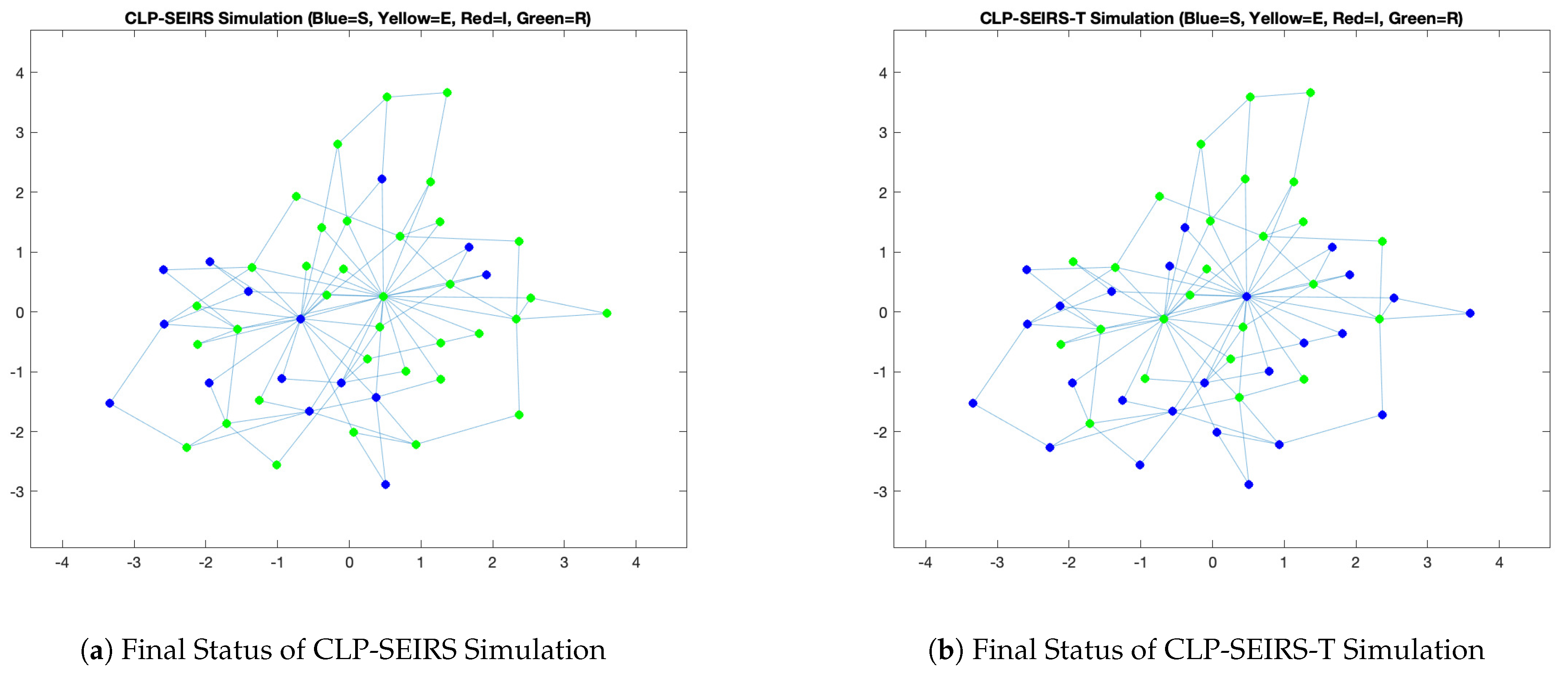
At the conclusion of the 50-step simulation, the overall distribution of node states differs markedly between the always-online network, as shown in Figure 2. A comparative examination of the node colors in the two figures reveals significant contrasts in the fractions of nodes remaining susceptible, recovered, exposed, and infectious:
In the CLP-SEIRS model (Figure 2a), very few nodes remain susceptible (blue) by the final time step, indicating that almost the entire network has been affected by the malware at some point. In stark contrast, the CLP-SEIRS-T outcome (Figure 2b) shows a much larger fraction of nodes still in the susceptible state by time step 50. A substantial portion of the nodes in Figure 2b are colored blue, indicating that approximately 25 nodes remain susceptible. This is a dramatic increase compared to the nearly negligible susceptible fraction in the always-online case.
The difference in recovered (green) nodes between the two scenarios complements this pattern. In Figure 2a, green nodes form the majority, signifying that most computers were infected during the simulation and subsequently recovered (gained temporary immunity). Indeed, the proportion of green nodes in the always-online case appears to be very high. In Figure 2b, however, green nodes are far less prevalent. Only a minority of nodes in the duty-cycled network end up in the recovered state by the final step. The sharp reduction of green nodes in the CLP-SEIRS-T figure, coupled with the abundance of blue nodes, indicates that many computers never contracted the virus in the temporally-active scenario, whereas in the always-online scenario nearly every computer eventually became infected and recovered.
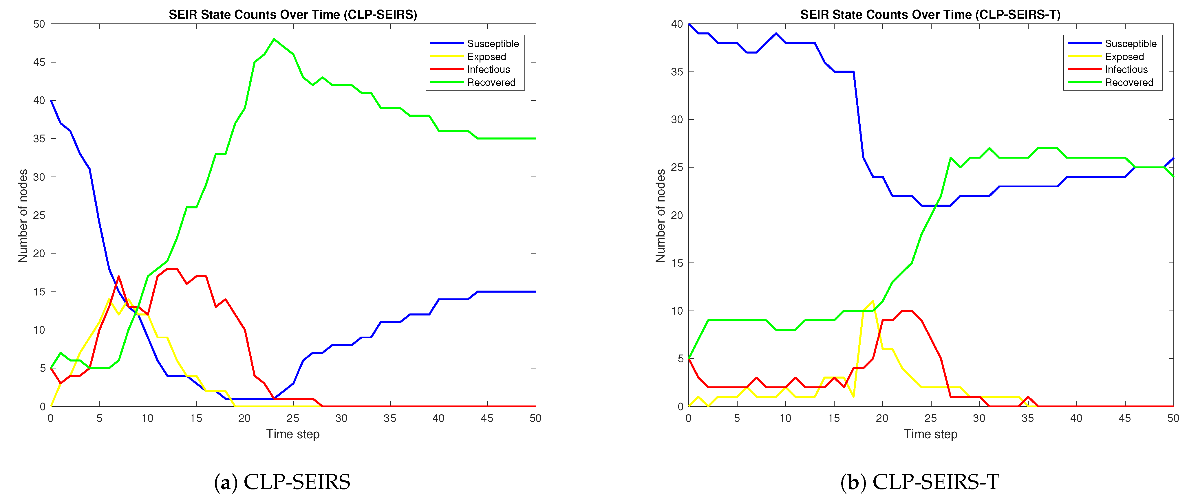
Figure 3 shows the state-time curves for CLP-SEIRS and CLP-SEIRS-T models, respectively. Each colored curve shows the number of nodes in the Susceptible (blue), Exposed (yellow), Infectious (red), and Recovered (green) compartments at each time step. Both simulations run for 50 discrete time steps on the same network.
In the fully-online CLP-SEIRS model (Figure 3a), the Infectious population (red curve) rises rapidly to a peak of 17 infectious individuals at t = 7 time steps. In the CLP-SEIRS-T model (Figure 3b), the infectious curve climbs more slowly and reaches a lower peak of 10 infectious individuals, occurring later at t = 22 . Thus, the peak prevalence of infection is substantially lower and the peak is delayed by 4 time steps in CLP-SEIRS-T compared to the baseline. The Exposed compartment (yellow curve) exhibits a similar delay: in CLP-SEIRS, the number of exposed individuals rises early with peaking around the same time as the infectious peak, whereas in CLP-SEIRS-T it remains low during the initial phase and only surges just before the delayed infectious peak. These shifts indicate that the infection spreads more slowly and never infects as many individuals simultaneously in the presence of periodic node inaccessibility.
The epidemic in the always-online model is short-lived and acute: after the peak, the number of infectious individuals declines to zero at t = 28 . By contrast, with periodic connectivity (CLP-SEIRS-T) the infection persists longer, with infectious individuals not disappearing until t = 36 . Moreover, the decline of the infectious curve in Figure 3b is not a smooth monotonic drop as in Figure 3a, but rather shows a stepwise pattern with minor fluctuations. These oscillations coincide with the on/off activation cycles: for example, a small resurgence in cases occurs when previously offline nodes come online and transmit or acquire infection. However, because contacts are regularly interrupted, such flare-ups are limited, and the overall trend still heads toward extinction. The net effect is that intermittent connectivity stretches out the epidemic curve while preventing the very sharp peak seen in the fully connected case.
In CLP-SEIRS, the susceptible population (blue curve) plummets from 40 to 1 within the first 18 time steps of the outbreak, indicating that almost the entire population becomes exposed in the initial wave of infection. By the end of the simulation, 15 individuals remain susceptible, implying that 70% of the population was infected and recovered at some point. In CLP-SEIRS-T, by contrast, the susceptible count declines much more gradually and never falls below 20 at its lowest point. There is a noticeable drop at t = 17 , coinciding with the belated outbreak peak, but even after this, 26 individuals remain susceptible at the end of the simulation. Thus, the time-periodic node availability leads to a significantly smaller epidemic overall, leaving a large fraction of the population uninfected, whereas the always-online scenario infects the majority of individuals.
The above differences in epidemic intensity and timing stem directly from the periodic unavailability of nodes in CLP-SEIRS-T. With only half of the nodes active at any given time (50% duty cycle), the effective contact rate is significantly reduced compared to a fully connected network. This intermittent connectivity acts like periodic social distancing: opportunities for transmission are limited and delayed. Consequently, fewer susceptible-infectious encounters occur per time step, slowing the spread and leading to a later, lower peak. The on/off pattern of connectivity also causes the epidemic to progress in spurts rather than one continuous wave. For instance, the surge in new exposures and infections in CLP-SEIRS-T happens when a batch of previously offline susceptible nodes all come online while infectious nodes are present, triggering a burst of transmissions. However, because infectious individuals also spend time offline, continuous transmission chains are broken. This extends the outbreak duration and prevents the infection from exploding as in the fully-online case. In effect, time-periodic node activity “flattens the curve”: the epidemic runs longer and flatter (lower peak, smaller final size), as expected when contact frequency is reduced.
In summary, the visual comparison of final states demonstrates that temporal activation of nodes has a profound dampening effect on malware propagation. The CLP-SEIRS-T model’s network ends with a high proportion of susceptible nodes and a low proportion of recovered nodes, indicating a limited outbreak, whereas the CLP-SEIRS model’s network ends with few susceptibles and a majority recovered, indicating an extensive outbreak. The presence of more ongoing cases in CLP-SEIRS-T further suggests that the epidemic is prolonged but less intense at any given time. These findings highlight that incorporating realistic node uptime patterns (in this case, a 50% duty cycle) can significantly alter epidemic outcomes, generally slowing down and reducing the spread of a computer virus. In practical terms, the temporal fragmentation of network connectivity in CLP-SEIRS-T confers a degree of protection to the network that is absent in the always-on scenario, thus emphasizing the importance of temporal factors in epidemiological modeling of malware spread.

3.2. Propagation Dynamics Under Varying Online Availability Less than 50%

We evaluate the propagation of a computer virus using the CLP-SEIRS-T model on a network of 100 nodes, as shown in Figure 4. The model parameters are set as follows: the intra-community infection rate β = 0.8 (transmission probability per contact on edges within the same community), the inter-community infection rate ρ = 0.3 (for contacts across communities), the exposed-to-infectious progression rate σ = 0.33 , the recovery rate γ = 0.05 , the immunity waning (reversion) rate ξ = 0.01 , and the secondary infection rate via a common neighbor λ = 0.2 . These parameters define a fairly virulent virus (high β ) with a short latent period (mean 1 / σ 3 time units), moderate recovery time (mean 1 / γ = 20 time units), and partial immunity that can be lost over time. The network topology incorporates community structure: nodes are partitioned into subgroups such that contacts within a community have a higher chance of infection ( β ) than contacts between communities ( ρ ). We assume an initial outbreak seed of about 10 nodes (10% of the network) set as infectious at t = 0 , with the remaining nodes initially susceptible (i.e., I ( 0 ) = 10 , S ( 0 ) = 90 , and E ( 0 ) = R ( 0 ) = 0 ).
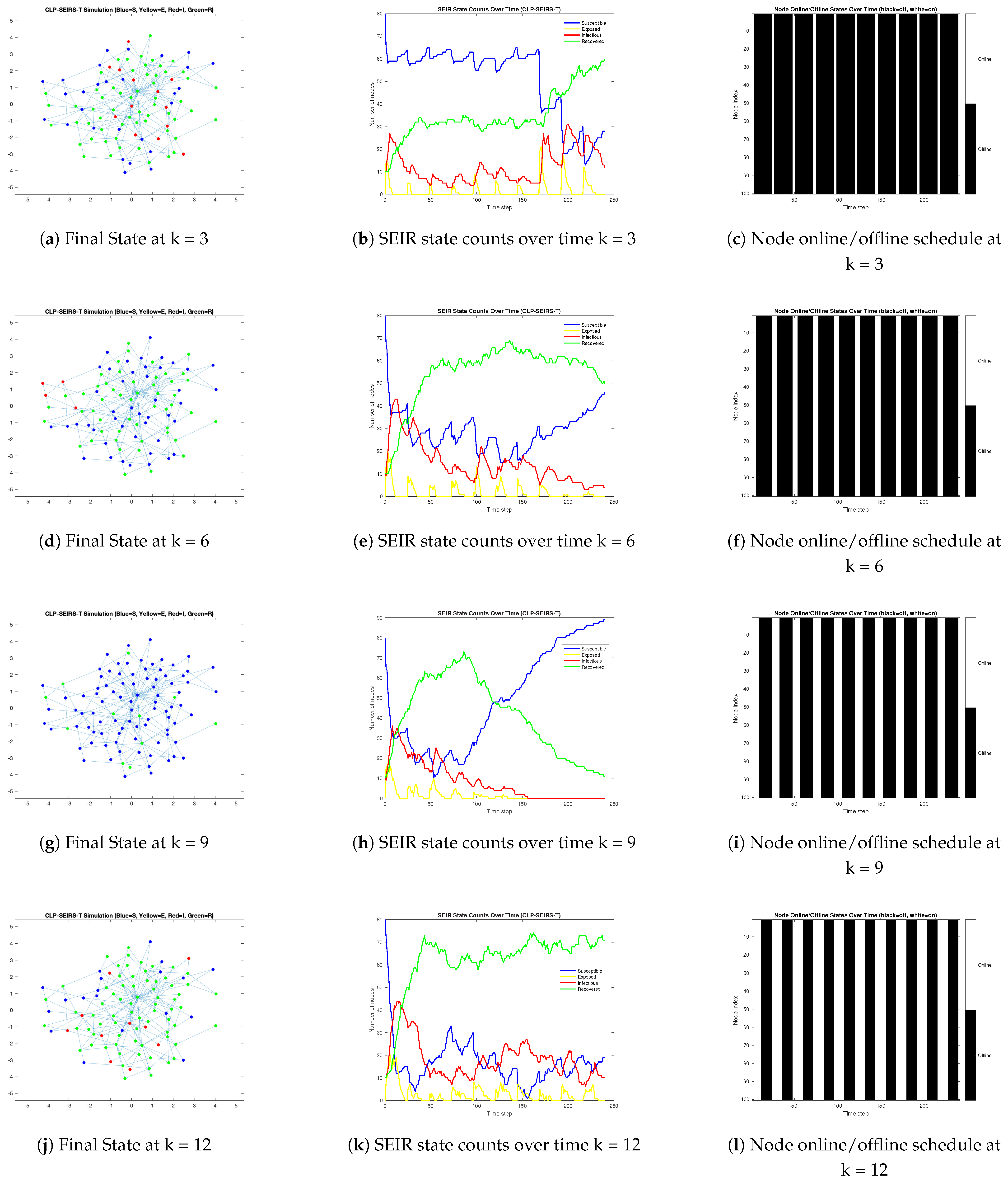
Each node’s connectivity to the network is periodic over a 24-h cycle. Specifically, every node is online for a fixed number of hours each day, and offline for the rest. We set the period to minPeriod = maxPeriod = 24 time steps, synchronizing daily cycles for all nodes with phase = 0. The fraction of time nodes are online is controlled by the parameter k, which represents the number of hours online in a 24-h cycle, so k / 24 is the online rate. We conduct four simulation scenarios with k = 3 , 6 , 9 , and 12, corresponding to online availability of 12.5%, 25%, 37.5%, and 50% of each day, respectively. In each scenario, all nodes share the same online/offline schedule (phase-aligned); for example, at k = 3 each node is online for 3 consecutive hours and offline for 21 h in every 24-h period. The simulations are run for 240 discrete time steps (approximately 10 cycles/days) to observe the full progression of the epidemic under each condition.
Figure 4 summarizes the results for the four different online rates. Subfigures (a), (d), (g), and (j) show the network topology and initial infection state for k = 3 , 6 , 9 , and 12, respectively. Nodes are colored by state (blue = susceptible, yellow = exposed, red = infectious, green = recovered) in these network snapshots. Subfigures (b), (e), (h), and (k) plot the temporal dynamics of the epidemic for each k value, showing the number of nodes in each state S, E, I, and R as a function of time. Finally, subfigures (c), (f), (i), and (l) illustrate the periodic online/offline schedule for all 100 nodes in each scenario. The width of the white bands in these panels corresponds to the duration of online activity k in each 24-step cycle. We next analyze the infection progression for each scenario in detail.
At the lowest availability ( k = 3 , Figure 4a–c), virus spread is slow and protracted. With only 3 h online per day (12.5% online rate), transmission opportunities are infrequent, and this significantly delays the outbreak. As shown in Figure 4b, the susceptible population S (blue curve) declines very gradually during the initial phase. In the first few 24-h cycles, only a small portion of susceptible nodes become infected. Correspondingly, the exposed (E, yellow) and infectious (I, red) counts rise slowly. The infectious population reaches an initial modest peak at a relatively late time compared to the higher-k scenarios, underscoring that the virus propagates at a subdued pace when nodes rarely come online. Many nodes remain susceptible through the early stages, and the epidemic fails to infect the entire network in one wave. As infectious nodes recover, the recovered population R (green curve) increases steadily, but since γ is small, this recovery is gradual. Because contacts are limited by the low online rate, the infection smolders for an extended period without explosive growth.
Notably, the k = 3 experiment exhibits multiple waves of infection. After the initial wave subsides, a substantial fraction of nodes are still susceptible. Over time, some recovered nodes lose immunity, returning to the susceptible pool. This, combined with the remaining susceptibles, allows the virus to resurge in a second outbreak at a later time. In Figure 4b, a pronounced second increase in I is seen around t = 169 , accompanied by a corresponding drop in S and rise in R. This secondary peak indicates that the virus, while initially suppressed, was never fully eradicated and could re-infect nodes once enough susceptibles accumulated. The epidemic is therefore drawn out: infectious individuals persist in the network until nearly t = 230 , much longer than in higher-k scenarios. In summary, when nodes are rarely online ( k = 3 ), the virus spreads sluggishly, peaks later at a lower level of infections, and lingers much longer in the population, with susceptible nodes only slowly being depleted and giving rise to delayed recurrent outbreaks.
Increasing the online time to k = 6 (25% online, Figure 4d–f) substantially accelerates the spread compared to k = 3 . With nodes active 6 h per day, transmission events are more frequent, leading to a much faster initial outbreak. Figure 4e shows that the susceptible count S (blue) drops steeply almost immediately. The infectious population I in red correspondingly surges to a high peak early in the simulation, in contrast to the delayed, lower peak observed when k = 3 . Specifically, I reaches its maximum well before t = 50 in the k = 6 case, indicating that the virus managed to infect many hosts in a short time once the contact rate was less constrained. The exposed category E (yellow) also rises more rapidly than in the k = 3 scenario, though it remains relatively small in magnitude (due to the short latent period, E quickly progresses to I).Following this initial explosive wave, the susceptible pool is significantly depleted, and many nodes have moved into R, as the green curve climbs sharply with the recovery of infected nodes.
After the first wave at k = 6 , the epidemic slows markedly—with fewer susceptibles available, new infections become rare. Figure 4e shows a small bump in the infectious curve around t = 106 . This corresponds to some recovered nodes losing immunity and re-entering the susceptible class, combined with any remaining never-infected individuals, which provides fuel for a resurgence. Because the number of susceptible nodes at this point is relatively low, this second outbreak is much weaker than the first; I increases only modestly and S dips slightly, indicating a limited spread. The second wave dies out quickly as the few newly infected nodes recover. By the end of the simulation, the infectious count has returned to nearly zero. Compared to k = 3 , the k = 6 scenario reaches a higher infection peak much sooner and resolves faster, with the majority of infections occurring in the initial outbreak. The overall epidemic duration is shorter, and although a small tail of infections persists (due to the second wave), it is less prolonged. Thus, a moderate increase in online time from 12.5% to 25% leads to a significantly quicker and more intense outbreak, followed by an earlier recovery phase, aligning with the expectation that more frequent connectivity accelerates epidemic dynamics.
When k is increased to 9 (37.5% online, Figure 4g–i), the network is online more than one-third of the time, yielding frequent contact opportunities and an even more rapid epidemic. In this scenario, we observe an almost immediate, explosive outbreak. As illustrated in Figure 4h, the susceptible population S (blue) plummets to 30 in the very early stage of the simulation—essentially, the majority of nodes become infected during the first 24-h cycle. The infectious count I (red) spikes to its maximum very quickly, far surpassing the peaks seen in the k = 3 and k = 6 cases. In fact, at k = 9 the virus infects nearly the entire network in one massive wave: the rapid decline of S and the simultaneous surge of I and R indicate that almost all susceptible nodes were exposed and transitioned to I, then many recovered, within a short timeframe. Because so many nodes gain immunity in this first wave, the susceptible pool is essentially exhausted by the time I starts to decline. As a result, there are no susceptibles left to sustain transmission, and the infection dies out once the initial cohort of infected nodes recovers. The recovered population R (green) correspondingly plateaus at a high level. With no infectious agents remaining in the system (and no new infections introduced), no second wave occurs for k = 9 . The epidemic is essentially over almost as soon as it began: a single, fast outbreak infects nearly everyone and then extinguishes. This outcome highlights that a high online fraction leads to both faster spread and faster disappearance of the virus—the peak infection load is reached very quickly and the network recovers in a much shorter time compared to lower k scenarios.
At k = 12 (50% online time, Figure 4j–l), nodes are online half of each cycle, representing the upper extreme of connectivity in our experiments. As expected, the initial spread is extremely rapid—comparable to the k = 9 case or even faster. Figure 4k shows that the susceptible population S (blue) drops to almost zero within the first cycle; virtually all susceptible nodes become infected in the initial burst. The infectious population I (red) skyrockets to a high peak immediately, and a large fraction of the network becomes recovered R (green) shortly thereafter. In terms of sheer speed and early impact, k = 12 produces the fastest and largest initial outbreak of all scenarios. However, an interesting dynamic emerges after this first wave: unlike the k = 9 case, the epidemic does not end after the initial peak, but instead goes through multiple smaller waves. This is evident in Figure 4k where, after the first peak of I falls, the red curve exhibits at least two subsequent rises (at t = 71 and t = 120 ). The presence of the secondary peak is due to the interplay of high connectivity and immunity loss. Because nodes are online so frequently, even a few remaining infectious individuals can easily contact others. After the first wave, while most nodes are in the recovered state, a fraction of those recovered begin to lose immunity. Given the continuous half-time online exposure, some of these newly susceptible nodes quickly become re-infected by the residual infectious nodes that survived the initial crash. In essence, the virus persists at low levels and reignites as soon as sufficient susceptible individuals are available, resulting in a second outbreak. Each successive wave is smaller than the previous one, due to the progressively reduced availability of susceptible individuals and is truncated more rapidly, as reflected by the diminishing peaks of I in Figure 4k. Thus, the k = 12 scenario demonstrates that maximal online connectivity leads to an immediate and intense outbreak, but can also sustain the virus through reinfections, causing a prolonged tail of infection albeit in diminishing waves. Importantly, even though the epidemic lingered through multiple flare-ups, the timing of these peaks is much earlier than in lower-k cases, and the overall time frame for the bulk of infections is compressed relative to scenarios with lower connectivity.

3.3. Propagation Dynamics Under Varying Online Availability Great than 50%

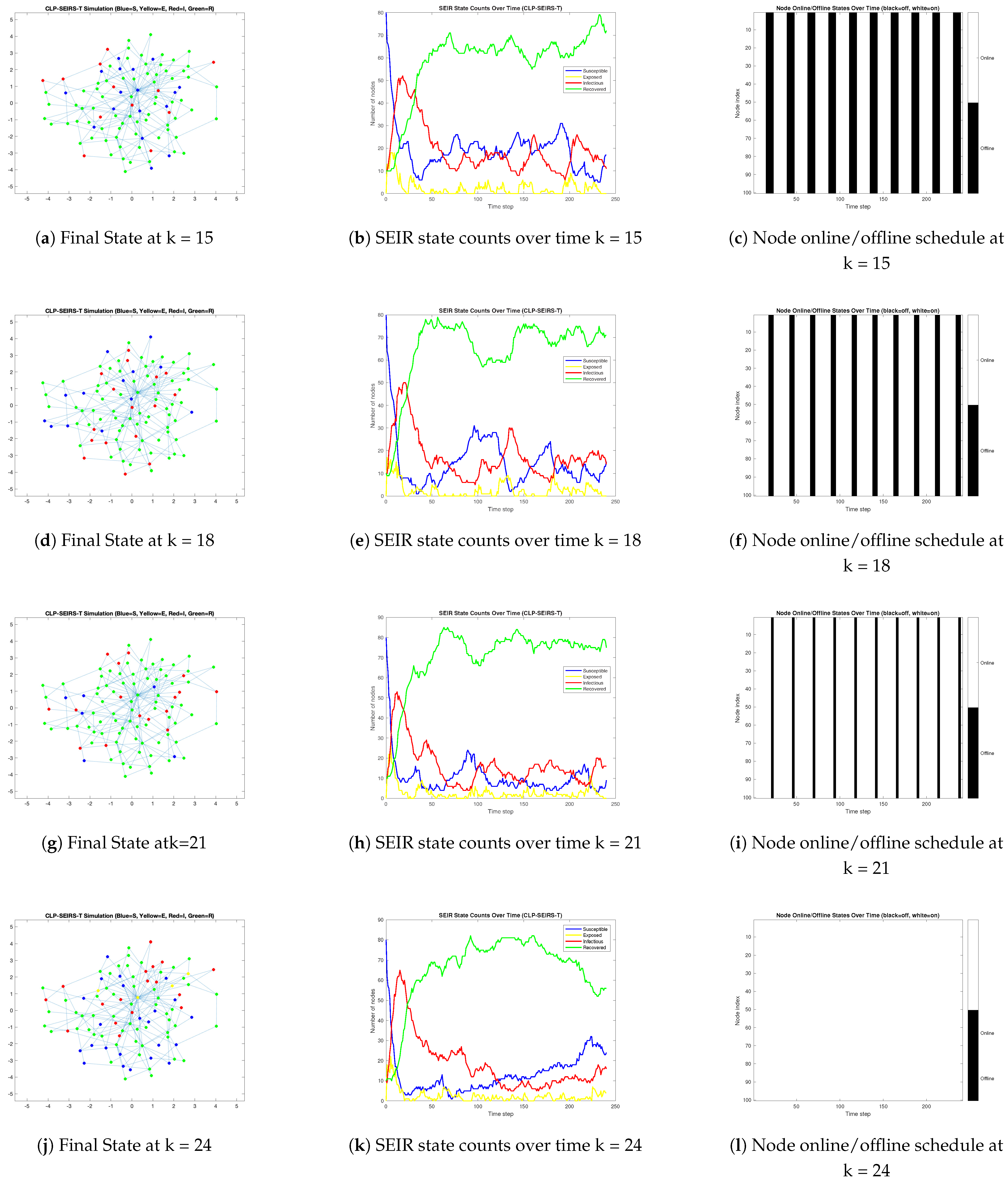
Figure 5 shows the simulation results for virus propagation under the CLP-SEIRS-T model at four different online rates, where k = 15 , 18 , 21 , and 24 out of 24.
In all four scenarios, because the online rate exceeds 50%, a self-sustaining epidemic outbreak is observed. Comparing across Figure 5a–d, several clear trends are observed as the online rate increases beyond 50%. Infection acceleration is evident: higher k values lead to a steeper rise in the number of infected nodes and a shorter time to reach the infection peak. For instance, the initial exponential growth rate of the epidemic is lowest for the k = 15 case and highest for k = 24 , in line with the effective contact rate scaling with the fraction of time online. With continuous connectivity (100% online), the epidemic growth closely resembles the classical fast epidemic scenario with maximal R 0 , whereas with 62.5% connectivity the growth is more gradual due to recurring halts in transmission. The time at which the peak number of infections occurs decreases notably as k increases. Likewise, the peak infection prevalence, defined as fraction of nodes simultaneously infectious at the peak, rises with k. In the high-connectivity simulations, a large fraction of nodes become infected in unison during the main wave, whereas in lower-k simulations the infections are spread out over time, yielding a lower concurrent infection count.
The outcomes also demonstrate more pronounced recovery saturation at higher online rates. By “recovery saturation,” we refer to the extent to which the recovered compartment R fills up by the end of the simulation, indicating how many individuals in total were infected at any point. In Figure 5k ( k = 24 ), R ( t ) reaches 56 by the final time, implying essentially every node went through the infection. In Figure 5h ( k = 21 ) a similar saturation is observed or at most a few individuals remain never infected. By contrast, in Figure 5b ( k = 15 ), R ( t ) reaches a lower asymptote by the end of the run; a noticeable fraction of nodes have not been infected, as indicated by a higher final S count. Although given a longer time the infection would likely continue to spread, within the observed timeframe the lower connectivity slowed the process such that herd immunity (or epidemic burnout) had not fully developed. This is also reflected in the susceptible curves: for higher k, S ( t ) is driven very close to zero at the height of the outbreak (indicating an almost complete consumption of susceptibles during the first wave), whereas for k = 15 the susceptible curve retains a non-zero value at its lowest point. Therefore, the degree of depletion of susceptible individuals is strongly dependent on the online fraction: more online time leads to more thorough exhausting of the susceptible pool in one major wave, pushing the system closer to its saturation point of full network infection.
In all cases, because the model includes waning immunity ( ξ = 0.01 ), recovered nodes gradually revert to the susceptible state over time (becoming susceptible again). However, the rate of return to susceptibility is very slow relative to the epidemic spread. In the high-k scenarios where the outbreak burns through the population quickly, there is a period after the initial wave where a large fraction of nodes are immune (in R) and only a few infectious individuals remain. During this post-peak phase, we expect a gradual trickle of nodes from R back to S. In the k = 24 case, because the infection dies out quickly after the peak, any nodes that lose immunity will become susceptible into an environment with no active infection, resulting in a temporary virus-free period. In Figure 5k, this is seen as R ( t ) plateauing and even slightly declining towards the end once the epidemic has effectively ended. If the simulation were continued further, a second wave would only occur if a reintroduction of infection or a few lingering infectious cases coincide with enough people having lost immunity. In contrast, at lower online rates (Figure 5b,e), the epidemic spread is more protracted, meaning that even as some recovered individuals become susceptible again, there may still be ongoing infections in the population. Indeed, for k = 15 , the infection persists throughout the simulation horizon, and by the end of the simulation there are still some infectious nodes circulating. This continuous presence of the virus, combined with slow immunity loss, can sustain a low-level epidemic state or generate subsequent smaller waves without external reintroduction. Thus, higher connectivity leads to a more acute but self-limiting outbreak, characterized by one dominant wave in which nearly all individuals are infected, followed by a cessation of infections, whereas slightly lower connectivity (but still >50%) produces a more drawn-out epidemic where infection can linger and take advantage of susceptibles regenerating over time.

3.4. Impact of Randomized Phase Online Patterns on CLP-SEIRS-T Dynamics

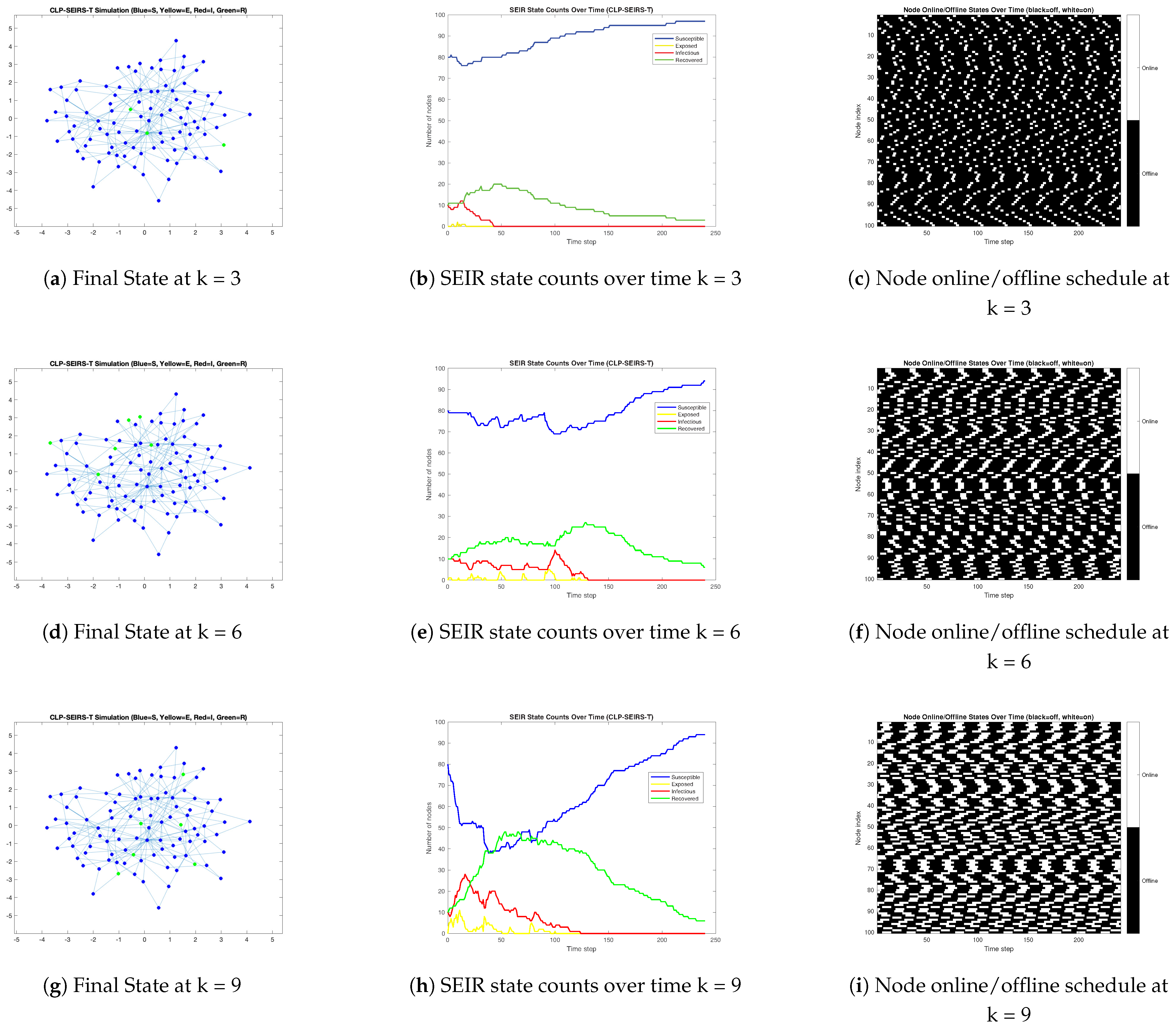
The simulation results under randomized online/offline phase shifts reveal marked differences in epidemic dynamics as the phase grouping k varies (Figure 6a–l). In all cases, the susceptible population (blue curves) initially declines when an outbreak occurs, reaching a distinct trough before rebounding as recovered nodes lose immunity and re-enter the susceptible pool. The timing and depth of these susceptible troughs depend strongly on k. For the lowest phase grouping, k = 3 (Figure 6a–c), the susceptible count experiences only a modest initial dip—dropping from 80 susceptible nodes to a minimum of 76 within the first few time steps—after which it steadily recovers. In contrast, at k = 6 (Figure 6d–f) the susceptible curve exhibits a deeper secondary trough: after an initial fall to ∼72 susceptibles by t = 51 , a more pronounced minimum of 69 susceptible nodes occurs later around t = 99 due to a second infection wave. As k increases further, the susceptible troughs become both deeper and more rapid. For k = 9 (Figure 6g–i), the first outbreak drives the susceptible count down to 51 at t = 130 . At the highest phase shift k = 12 (Figure 6j–l), the susceptible population plummets to its lowest level—13 out of 100 nodes—almost immediately. Notably, the k = 12 case shows multiple recurring troughs of comparable magnitude. This indicates that larger k not only yields a more severe initial susceptibility drop, but also sustains repeated troughs over time. By comparison, for small k (e.g., k = 3 ), the susceptible fraction never falls below roughly three-quarters of the network, and no later trough comes close to the initial dip. Thus, increasing k leads to progressively lower susceptible minima and enables these minima to recur in later phases of the simulation rather than only at the outset.
The recovered node trajectories (green curves) demonstrate that higher k values correspond to substantially larger outbreak sizes, as reflected in the peak number of recovered computers. At k = 3 (Figure 6b), the recovered count rises to a modest peak of 20 nodes during the single main outbreak, and thereafter declines toward zero as those recovered nodes gradually lose immunity. Increasing the phase groups to k = 6 yields a slightly higher recovered peak of 27 concurrent recovered nodes (25%) during the second wave (Figure 6e). When k = 9 , the outbreak grows much larger: the recovered curve climbs to 45 at its highest point. For k = 12 , the immunity burden on the network becomes even more pronounced—the first epidemic wave alone pushes the recovered count to 71 nodes at its apex as shown in Figure 6k). In fact, each successive wave at k = 12 reaches a high recovered level on the order of 60–70 nodes, indicating that a majority of the network cycles through the infected and recovered states multiple times. This trend of increasing peak recovered count with k is evident: the maximum concurrent recovered population rises by roughly a factor of 3.5 between k = 3 and k = 12 (from 20 to 71 nodes). Higher k thus clearly exacerbates the epidemic’s reach, as seen by the greater heights of the green curves.The growth and decay patterns of R ( t ) therefore underscore that larger phase-shift diversity (k) enables more computers to be infected over time, yielding higher and repeated peaks in the recovered population.
Another key trend is the difference in convergence speed and infection suppression across these scenarios. Lower values of k lead to faster die-out of the virus and quicker return to a healthy (susceptible) state for the network. In the k = 3 case, the infection is rapidly extinguished: the infectious node count (red curve in Figure 6b) falls to zero soon after the initial outbreak. Correspondingly, the system approaches an infection-free equilibrium by mid-simulation—the susceptible curve in Figure 6b flattens out and approaches 95 nodes (complete susceptibility) by t = 150 , while the recovered count dwindles toward zero, indicating full convergence to the virus-free state. A similar but slightly slower suppression is observed at k = 6 : although this case exhibits two infection waves, by t = 130 the infectious count drops to zero after the second wave (Figure 6e) and no further outbreaks occur. Thus, the virus is effectively cleared from the network by the midpoint of the simulation for k = 6 , and afterwards the curves simply relax as remaining recovered nodes revert to susceptible. In the k = 9 scenario, the epidemic is more intense initially but still eventually dies out. The large first wave rapidly infects a significant portion of the network. Beyond t = 125 , no major new infections arise—the system enters a long tail where the recovered population decays and susceptible count gradually rebounds toward full capacity. By the end of the simulation ( t = 250 ), the k = 9 case has essentially returned to a near-fully susceptible state, indicating successful suppression of the virus after the initial outbreak burnout. In stark contrast, the k = 12 network fails to reach a steady state within the simulated time due to repeated infection resurgences. As shown in Figure 6k, whenever the infectious count begins to decline, a new subset of susceptible nodes comes online because of the many phase-shift groups, seeding another wave before the infection can be completely eliminated. Consequently, the infectious population never stays at zero for long—multiple red spikes are seen throughout the k = 12 timeline—and at t = 250 there are still 15 active infections with a new upswing underway. The susceptible and recovered fractions likewise continue to oscillate rather than converging. In summary, higher k values markedly prolong the epidemic and impede complete infection suppression. The k = 12 case exhibits sustained oscillatory dynamics with the virus persisting up to the simulation horizon, whereas the lower-k cases (especially k = 3 ) show rapid convergence to an infection-free condition after one or two waves. This indicates that increasing the number of randomized phase offsets (larger k) slows down the convergence toward the virus-free equilibrium and allows the malware to linger via successive flare-ups, as opposed to the swift eradication observed under smaller k values.

4. Conclusions and Future Work

4.1. Conclusions

In this paper, we presented the CLP-SEIRS-T model, an enhanced epidemiological framework for malware propagation that integrates community structure (clustered networks), link prediction (emerging connections), and temporal node activation (periodic online/offline cycles). This unified model addresses several gaps in prior work by simultaneously accounting for heterogeneous network topology, evolving connectivity, and non-continuous communication patterns.The conclusions are as follows:
  • Strong community structure can localize infections and delay inter-community spread, especially when combined with limited or intermittent cross-community contacts. We observed that when nodes follow periodic duty cycles, malware spread is substantially slowed and fragmented. Lower online availability effectively “flattens” the infection curve: outbreaks unfold over longer periods and peak at lower infection levels, often leaving a considerable portion of nodes uninfected. In particular, imposing asynchronous or staggered online schedules across different communities further confined the virus, as misaligned active periods meant that an outbreak in one cluster often failed to synchronize with activity in others.
  • When connectivity is near-continuous or highly synchronous, we found that contagion dynamics resemble those in classic epidemic models on homogeneous networks. High overall contact rates (e.g., nodes online nearly 100% of the time) led to fast, explosive outbreaks that infected almost the entire network in a single wave. Community boundaries offer little resistance in such scenarios, as even a small number of inter-community links allow the virus to traverse between clusters when nodes are continuously active. Our numerical simulatoin results revealed a clear threshold effect in node availability: beyond a certain fraction of time online, the malware spread becomes rampant and difficult to contain, whereas below that threshold the outbreak remains partial or dies out after limited waves. Moreover, synchronized activation across nodes produced one dominant outbreak peak followed by die-out, whereas staggered (asynchronous) activation allowed the infection to persist via multiple smaller waves. In the asynchronous cases, the malware could re-emerge when previously offline devices came online, resulting in protracted, oscillatory epidemic behavior. This result underlines the importance of incorporating realistic, non-synchronized usage patterns into virus spread models, as they can sustain contagion even when instantaneous infection rates are low.
  • By incorporating a common-neighbor link-prediction mechanism, the CLP-SEIRS-T model captures indirect infection pathways that would be missed in static-network models. Even if two devices are not directly connected, our model allows malware transmission if they share enough neighbors. We found that these predicted links can significantly increase the reach of an outbreak: infections were able to jump across network gaps and infect otherwise isolated communities via “future” connections. Including this effect effectively lowers the epidemic threshold and raises the final fraction of infected nodes, indicating that traditional models which ignore potential link formation may underestimate the true risk and extent of malware spread. From a defensive standpoint, this finding suggests that network administrators should not only secure existing links but also be mindful of likely future connections.
Collectively, the results indicate that enhancing community modularity, reducing online availability, adopting asynchronous or staggered online schedules across communities, and minimizing common-neighbor connections represent effective strategies for mitigating or preventing malware propagation in urban communication networks.

4.2. Future Work and Extensions

  • Heterogeneous Duty Cycles: In this study we assumed all nodes share the same duty cycle κ . However, real networks often contain devices with widely varying activity levels. The model can readily accommodate different κ i values for each node, which would lead to interesting changes in propagation dynamics. For example, a device that is almost always online could act as a super-spreader and accelerate the overall malware spread, whereas a device that rarely comes online would hardly participate in transmission, effectively serving as a “firebreak”. Future work can investigate how different distributions of duty cycles affect outbreak outcomes, assessing the model’s sensitivity to heterogeneous node availability.
  • Adaptive Link-Prediction Parameter: In our simulations, the link-prediction infection rate λ was treated as a constant. In reality, however, λ might not be fixed and could vary over time or with network conditions. Future extensions of the model could tie λ to network metrics, allowing it to adjust dynamically as the epidemic unfolds and the network structure evolves.
  • Empirical Validation: At present, due to the lack of publicly available datasets on malware propagation in urban communication networks, the CLP-SEIRS-T model has only been evaluated via simulations on synthetic networks. In the future, we plan to validate the model against real-world data. One possible approach is to apply the model to network traffic traces from actual systems, or to conduct controlled experiments in a virtual machine-based network environment to simulate real malware spread scenarios.
  • Stochastic Node Activation: We assumed periodic, deterministic online/offline patterns for nodes to facilitate analysis. In reality, however, node activity can be stochastic. The CLP-SEIRS-T framework can be extended to incorporate random activation times or use an “activity-driven” network model. We anticipate that randomizing node activation would, on average, still mitigate malware spread similar to having a duty cycle, but the detailed temporal dynamics may differ. Future work can explore how non-periodic, probabilistic connectivity patterns affect malware propagation.
  • Weighted and Directed Networks: Our model assumed an undirected, unweighted network, but it can be extended to directed or weighted graphs. In a directed network, one can account for asymmetry in transmission (different infection probabilities in each direction of a link); in a weighted network, the infection rate of an edge can be made proportional to its weight. These extensions would introduce additional parameters and complexity, but would allow the model to apply to a wider range of communication systems. It will be valuable in future work to study how asymmetric or weighted connectivity influences malware spread.
  • Scalability and Complexity: We recognize that simulating CLP-SEIRS-T on very large networks (with more than 10 4 nodes) could be computationally demanding. At each time step the model must evaluate transmissions via direct and predicted links, leading to a complexity on the order of O ( N 2 ) in the worst case. While our current implementation easily handles networks of size N = 100 , scaling to much larger networks would require optimized algorithms or parallel computing. For real-time outbreak forecasting on extremely large networks, further simplifications might be necessary to reduce computational cost. In future work we will explore more efficient implementations to improve the model’s applicability to large-scale networks.

Author Contributions

Conceptualization, G.C. and Q.S.; methodology, G.C. and Y.L.; software, Y.L.; validation, G.C. and Y.L.; formal analysis, G.C. and Y.L.; investigation, G.C. and Y.L.; resources, G.C. and Y.L.; data curation, G.C.; writing–original draft preparation, G.C.; writing–review and editing, G.C. and Y.L. and Q.S.; visualization, G.C.; supervision, G.C. and Y.L.; project administration, Y.L.; funding acquisition, G.C. and Q.S. and Y.L. All authors have read and agreed to the published version of the manuscript.

Funding

This study was supported by the Guizhou University Doctoral Fund [grant (2022) 34], Basic Research Project of Guizhou University (grant [2023] 42), Guizhou Provincial Basic Research Program (Natural Science) qiankehejichu-MS [2025] 684.

Data Availability Statement

The original contributions presented in this study are included in the article. Further inquiries can be directed to the corresponding author.

Conflicts of Interest

The authors declare no conflict of interest.

Abbreviation

The following abbreviation is used in this manuscript:
CLP-SEIRS-TClustered Link-Prediction SEIRS Model with Temporal Node Activation

References

  1. Ghafur, S.; Kristensen, S.; Honeyford, K.; Martin, G.; Darzi, A.; Aylin, P. A retrospective impact analysis of the WannaCry cyberattack on the NHS. NPJ Digit. Med. 2019, 2, 98. [Google Scholar] [CrossRef] [PubMed]
  2. Tsvetanov, T.; Slaria, S. The effect of the Colonial Pipeline shutdown on gasoline prices. Econ. Lett. 2021, 209, 110122. [Google Scholar] [CrossRef]
  3. Zhang, X.; Upton, O.; Beebe, N.L.; Choo, K.K.R. IoT Botnet Forensics: A Comprehensive Digital Forensic Case Study on Mirai Botnet Servers. Forensic Sci.-Int.-Digit. Investig. 2020, 32, 300926. [Google Scholar] [CrossRef]
  4. Zhang, Y.; Jiang, L.; Ewe, H.T. A Novel Data-Driven Modeling Method for the Spatial Temporal Correlated Complex Sea Clutter. IEEE Trans. Geosci. Remote Sens. 2022, 60, 1–11. [Google Scholar] [CrossRef]
  5. Ding, Y.; Xiao, Y.; Xie, J.; Zhang, T. A time-varying transition channel model for air-ground communication. In Proceedings of the 2017 IEEE/AIAA 36th Digital Avionics Systems Conference (DASC), St. Petersburg, FL, USA, 17–21 September 2017; pp. 1–8. [Google Scholar] [CrossRef]
  6. Zhang, Y.; Jiang, L. A Novel Data-Driven Analysis Method for Electromagnetic Radiations Based on Dynamic Mode Decomposition. IEEE Trans. Electromagn. Compat. 2020, 62, 1443–1450. [Google Scholar] [CrossRef]
  7. Zhang, Y.; Jiang, L. A Novel Data-Driven Scheme for the Ship Wake Identification on the 2-D Dynamic Sea Surface. IEEE Access 2020, 8, 69593–69600. [Google Scholar] [CrossRef]
  8. Hethcote, H. The mathematics of infectious diseases. SIAM Rev. 2000, 42, 599–653. [Google Scholar] [CrossRef]
  9. Mishra, B.K.; Pandey, S.K. Dynamic model of worm propagation in computer network. Appl. Math. Model. 2014, 38, 2173–2179. [Google Scholar] [CrossRef]
  10. Kephart, J.; White, S. Measuring and modeling computer virus prevalence. In Proceedings of the 1993 IEEE Computer Society Symposium on Research in Security and Privacy, Oakland, CA, USA, 24–26 May 1993; pp. 2–15. [Google Scholar] [CrossRef]
  11. Staniford, S.; Paxson, V.; Weaver, N. How to Own the Internet in Your Spare Time. In Proceedings of the 11th USENIX Security Symposium, San Francisco, CA, USA, 5–9 August 2002; pp. 149–167. [Google Scholar]
  12. Zou, C.C.; Towsley, D.; Gong, W. Modeling and simulation study of the propagation and defense of internet e-mail worms. IEEE Trans. Dependable Secur. Comput. 2007, 4, 105–118. [Google Scholar] [CrossRef]
  13. Ing, J.; Pavlovskaia, E.; Wiercigroch, M.; Banerjee, S. Bifurcation analysis of an impact oscillator with a one-sided elastic constraint near grazing. Phys. D Nonlinear Phenom. 2010, 239, 312–321. [Google Scholar] [CrossRef]
  14. Rathie, P.N.; Coutinho, M.; Sousa, T.R.; Rodrigues, G.S.; Carrijo, T.B. Stable and generalized-t distributions and applications. Commun. Nonlinear Sci. Numer. Simul. 2012, 17, 5088–5096. [Google Scholar] [CrossRef]
  15. Xiong, S.; Yao, Y.; Berry, M.; Qi, H.; Cao, Q. Frequent traffic flow identification through probabilistic bloom filter and its GPU-based acceleration. J. Netw. Comput. Appl. 2017, 87, 60–72. [Google Scholar] [CrossRef]
  16. Musa, A.; Almohannadi, H.; Alhamar, J. Malware Propagation Modelling in Peer-to-Peer Networks: A Review. In Proceedings of the 2018 6th International Conference on Future Internet of Things and Cloud Workshops (FiCloudW), Barcelona, Spain, 6–8 August 2018; pp. 198–202. [Google Scholar] [CrossRef]
  17. Liu, W.; Zhong, S. Modeling and analyzing the dynamic spreading of epidemic malware by a network eigenvalue method. Appl. Math. Model. 2018, 63, 491–507. [Google Scholar] [CrossRef]
  18. Nguyen, B. Modelling Cyber Vulnerability using Epidemic Models. In Proceedings of the 7th International Conference on Simulation and Modeling Methodologies, Technologies and Applications, SIMULTECH 2017, Madrid, Spain, 26–28 July 2017; SCITEPRESS: Setubal, Portugal, 2017; pp. 232–239. [Google Scholar] [CrossRef]
  19. Boccaletti, S.; Latora, V.; Moreno, Y.; Chavez, M.; Hwang, D.U. Complex networks: Structure and dynamics. Phys. Rep. Rev. Sect. Phys. Lett. 2006, 424, 175–308. [Google Scholar] [CrossRef]
  20. Pastor-Satorras, R.; Vespignani, A. Epidemic spreading in scale-free networks. Phys. Rev. Lett. 2001, 86, 3200–3203. [Google Scholar] [CrossRef] [PubMed]
  21. Pastor-Satorras, R.; Castellano, C.; Van Mieghem, P.; Vespignani, A. Epidemic processes in complex networks. Rev. Mod. Phys. 2015, 87, 925–979. [Google Scholar] [CrossRef]
  22. Wang, Y.; Chakrabarti, D.; Wang, C.; Faloutsos, C. Epidemic spreading in real networks: An eigenvalue viewpoint. In Proceedings of the 22nd International Symposium on Reliable Distributed Systems, Florence, Italy, 6–8 October 2003; pp. 25–34. [Google Scholar] [CrossRef]
  23. Newman, M. Spread of epidemic disease on networks. Phys. Rev. E 2002, 66. [Google Scholar] [CrossRef]
  24. Cohen, R.; Havlin, S.; ben Avraham, D. Efficient immunization strategies for computer networks and populations. Phys. Rev. Lett. 2003, 91, 247901. [Google Scholar] [CrossRef]
  25. Newman, M. The structure and function of complex networks. SIAM Rev. 2003, 45, 167–256. [Google Scholar] [CrossRef]
  26. Dorogovtsev, S.; Goltsev, A.; Mendes, J.; Samukhin, A. Spectra of complex networks. Phys. Rev. E 2003, 68, 046109. [Google Scholar] [CrossRef]
  27. Chakrabarti, D.; Faloutsos, C. Graph mining: Laws, generators, and algorithms. ACM Comput. Surv. 2006, 38, A1–A69. [Google Scholar] [CrossRef]
  28. Nadini, M.; Sun, K.; Ubaldi, E.; Starnini, M.; Rizzo, A.; Perra, N. Epidemic spreading in modular time-varying networks. Sci. Rep. 2018, 8, 2352. [Google Scholar] [CrossRef] [PubMed]
  29. Nematzadeh, A.; Ferrara, E.; Flammini, A.; Ahn, Y.Y. Optimal Network Modularity for Information Diffusion. Phys. Rev. Lett. 2014, 113, 088701, Erratum in Phys. Rev. Lett. 2014, 113, 259901. [Google Scholar] [CrossRef] [PubMed]
  30. Granell, C.; Gomez, S.; Arenas, A. Dynamical Interplay between Awareness and Epidemic Spreading in Multiplex Networks. Phys. Rev. Lett. 2013, 111, 128701. [Google Scholar] [CrossRef]
  31. Holme, P.; Saramaki, J. Temporal networks. Phys. Rep. Rev. Sect. Phys. Lett. 2012, 519, 97–125. [Google Scholar] [CrossRef]
  32. Masuda, N.; Miller, J.C.; Holme, P. Concurrency measures in the era of temporal network epidemiology: A review. J. R. Soc. Interface 2021, 18. [Google Scholar] [CrossRef]
  33. Valdano, E.; Ferreri, L.; Poletto, C.; Colizza, V. Analytical Computation of the Epidemic Threshold on Temporal Networks. Phys. Rev. X 2015, 5, 021005. [Google Scholar] [CrossRef]
  34. Rocha, L.E.C.; Blondel, V.D. Bursts of Vertex Activation and Epidemics in Evolving Networks. PLoS Comput. Biol. 2013, 9, e1002974. [Google Scholar] [CrossRef]
  35. Williams, O.E.; Lino, F.; Latora, V. Effects of memory on spreading processes in non-Markovian temporal networks. New J. Phys. 2019, 21, 043028. [Google Scholar] [CrossRef]
  36. Perra, N.; Goncalves, B.; Pastor-Satorras, R.; Vespignani, A. Activity driven modeling of time varying networks. Sci. Rep. 2012, 2, 469. [Google Scholar] [CrossRef]
  37. Sejunti, M.I.; Taylor, D.; Masuda, N. A Parrondo paradox in susceptible-infectious-susceptible dynamics over periodic temporal networks. Math. Biosci. 2024, 378, 109336. [Google Scholar] [CrossRef] [PubMed]
  38. Liben-Nowell, D.; Kleinberg, J. The link-prediction problem for social networks. J. Am. Soc. Inf. Sci. Technol. 2007, 58, 1019–1031. [Google Scholar] [CrossRef]
  39. Lu, L.; Zhou, T. Link prediction in complex networks: A survey. Phys. A-Stat. Mech. Its Appl. 2011, 390, 1150–1170. [Google Scholar] [CrossRef]
  40. Moore, S.; Rogers, T. Predicting the Speed of Epidemics Spreading in Networks. Phys. Rev. Lett. 2020, 124, 068301. [Google Scholar] [CrossRef]
  41. Gross, T.; D’Lima, C.J.D.; Blasius, B. Epidemic dynamics on an adaptive network. Phys. Rev. Lett. 2006, 96, 208701. [Google Scholar] [CrossRef]
  42. Shaw, L.B.; Schwartz, I.B. Enhanced vaccine control of epidemics in adaptive networks. Phys. Rev. E 2010, 81, 046120. [Google Scholar] [CrossRef]
  43. Li, R.; Guo, X. Dynamics of a Stochastic SEIR Epidemic Model with Vertical Transmission and Standard Incidence. Mathematics 2024, 12, 359. [Google Scholar] [CrossRef]
  44. Hernandez Guillen, J.D.; Martin del Rey, A.; Hernandez Encinas, L. Study of the stability of a SEIRS model for computer worm propagation. Phys. A-Stat. Mech. Its Appl. 2017, 479, 411–421. [Google Scholar] [CrossRef]
  45. Hosseini, S.; Zandvakili, A. The SEIRS-C model of information diffusion based on rumour spreading with fuzzy logic in social networks. Int. J. Comput. Math. 2022, 99, 1918–1940. [Google Scholar] [CrossRef]
  46. Zhang, Z.; Yang, H. Stability and Hopf Bifurcation in a Delayed SEIRS Worm Model in Computer Network. Math. Probl. Eng. 2013, 2013, 319174. [Google Scholar] [CrossRef]
  47. Asadi, E.; Hosseini, S. A clustered-LPSEIRS malware propagation model in complex networks. Appl. Netw. Sci. 2024, 9, 62. [Google Scholar] [CrossRef]
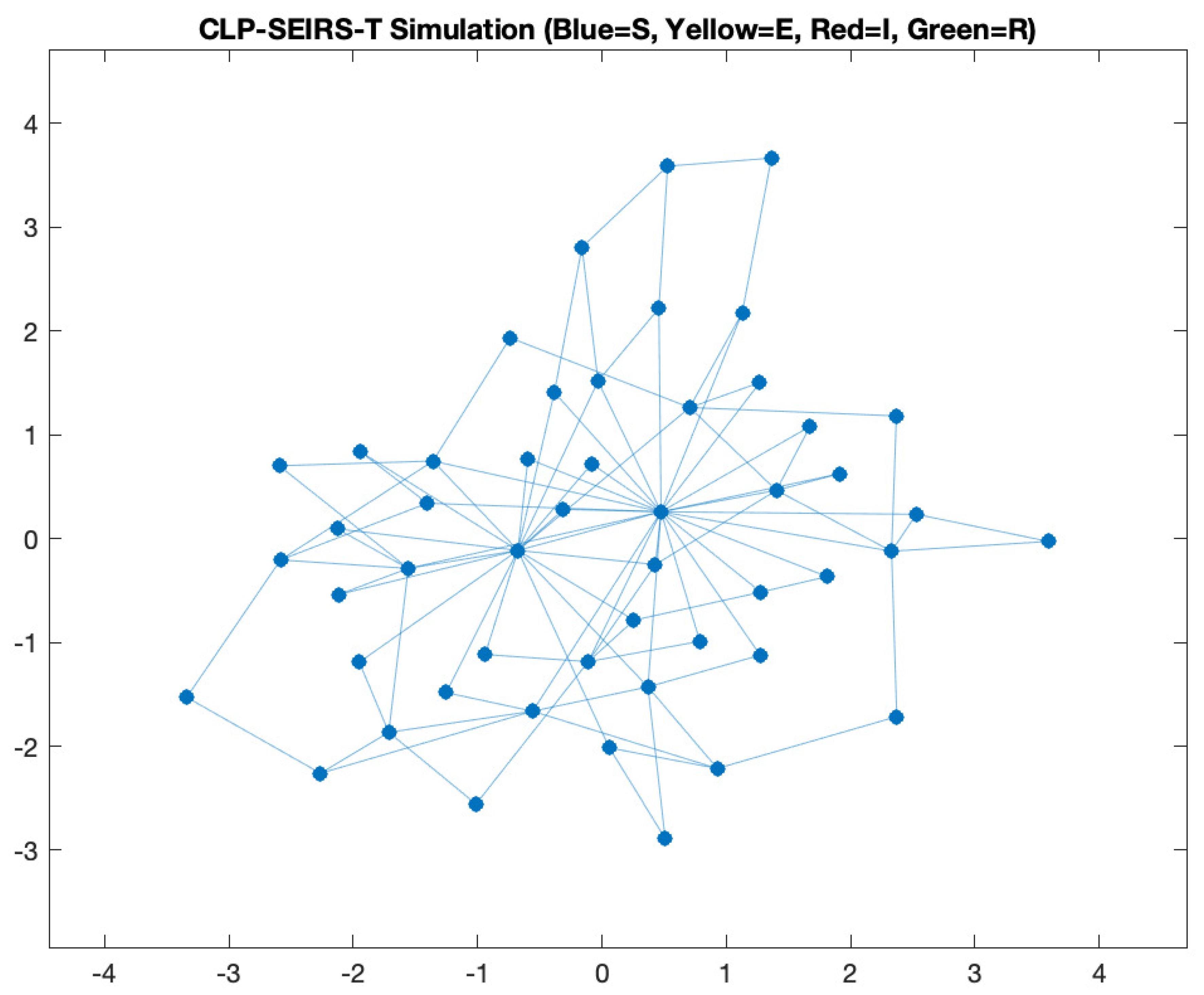
Figure 1. CLP-SEIRS-T simulation network.
Appliedmath 05 00128 g001
Figure 2. Comparison of CLP-SEIRS and CLP-SEIRS-T results: final state network diagrams.
Appliedmath 05 00128 g002
Figure 3. Infection state curves.
Appliedmath 05 00128 g003
Figure 4. CLP-SEIRS-T simulation results under varying online rates ( κ = k / 24  50%).
Appliedmath 05 00128 g004
Figure 5. CLP-SEIRS-T simulation results under varying online rates ( κ = k / 24 > 50 %).
Appliedmath 05 00128 g005
Figure 6. CLP-SEIRS-T simulation results under varying online rates with random on/off phases ( κ = k / 24 ).
Appliedmath 05 00128 g006aAppliedmath 05 00128 g006b
Table 1. Key notations and parameters in CLP-SEIRS-T.
SymbolDescription
NTotal number of nodes (individuals) in the network.
A i j Adjacency matrix entry (1 if edge between i , j exists, 0 otherwise).
β Infection rate for intra-community contacts.
ρ Infection rate for inter-community contacts.
λ Infection rate for predicted links
σ Progression rate from Exposed (E) to Infectious (I)
γ Recovery rate from Infectious (I) to Recovered (R)
ξ Immunity waning rate from Recovered (R) back to Susceptible (S).
T i Period of node i’s activity cycle (in discrete time steps).
p i ( t ) Periodic online status function for node i at time t.
ϕ i Phase offset of node i’s activity cycle (phase of initial activation).
κ Duty cycle (fraction of each period that node i is online).
Disclaimer/Publisher’s Note: The statements, opinions and data contained in all publications are solely those of the individual author(s) and contributor(s) and not of MDPI and/or the editor(s). MDPI and/or the editor(s) disclaim responsibility for any injury to people or property resulting from any ideas, methods, instructions or products referred to in the content.