Abstract
In this research work, we proposed and studied a fractional-order model for Human African Trypanosomiasis (HAT) disease transmission, incorporating three control strategies: health education campaigns, prevention measures, and use of insecticides. The theoretical analysis of the model was presented, including the computation of disease-free equilibrium and basic reproduction number. We performed the stability analysis of the model and the results showed that the disease-free equilibrium point was locally asymptotically stable whenever and unstable when . Furthermore, we performed parameter estimation of the model using HAT-reported cases in Tanzania. The results showed that fractional-order model had a better fit to the real data compared to the classical integer-order model. Sensitivity analysis of the basic reproduction number was performed using computed partial rank correlation coefficients to assess the effects of parameters on HAT transmission. Additionally, we performed numerical simulations of the model to assess the impact of memory effects on the spread of HAT. Overall, we observed that the order of derivatives significantly influences the dynamics of HAT transmission in the population. Moreover, we simulated the model to assess the effectiveness of proposed control strategies. We observed that the use of insecticides and prevention measures have the potential to significantly reduce the spread of HAT within the population.
Keywords:
Human African Trypanosomiasis; fractional-order model; sensitivity analysis; parameter estimation; numerical simulations; insecticide use MSC:
92B05; 93A30; 93C15
1. Introduction
Human African Trypanosomiasis (HAT), commonly listed as one of the neglected tropical diseases in Africa, is caused by protozoans of the genus Trypanosoma. The disease is transmitted to humans through the bite of infected tsetse flies (genus Glossina), which become carriers after feeding on infected persons or animals [1]. These vectors are found exclusively in sub-Saharan Africa [2]. HAT is endemic in rural areas, with individuals involved in agriculture, livestock, and hunting being the most at risk due to their proximity to tsetse fly habitats [3]. The disease progresses in two stages: the first presents with symptoms such as headaches and fever, which can last for years, while the second stage typically involves neuropsychiatric complications, such as sleep disturbances, hence the term ‘sleeping sickness’. Without treatment, the disease is often fatal [4]. Infected individuals may remain asymptomatic for months or years, and symptoms such as fever, irritability, fatigue, and swollen lymph nodes usually emerge after the disease has affected the central nervous system. In advanced stages, patients may experience confusion, skin rashes, personality changes, and other neurological impairments [5].
HAT is caused by two subspecies of Trypanosoma brucei: T. b. gambiense (TBG) and T. b. rhodesiense (TBR). TBG, responsible for 92% of all cases, causes a chronic illness prevalent in 24 countries across West and Central Africa [6]. In contrast, TBR, which causes a fast-progressing acute illness, is responsible for 8% of cases and is found in 13 countries in Eastern and Southern Africa [7]. Despite efforts to eliminate HAT by 2030, the disease remains a major public health issue in countries such as the Democratic Republic of Congo, Angola, Gabon, Guinea, Malawi, and South Sudan [8]. HAT continues to cause significant death and disability in sub-Saharan Africa, especially in remote areas where health access is limited. Treatment options vary by stage and parasite type: stage 1 of TBR is treated with suramin or pentamidine, while melarsoprol—despite its high toxicity—remains the main drug for advanced-stage infections [9]. Existing treatments require long courses of injections and are associated with serious side effects.
Mathematical models have been instrumental in studying vector-borne disease dynamics and control [10]. A foundational model by Rogers et al. [11] has been extended by numerous researchers, including those studying nonlinear incidence rates, which better capture real-world saturation effects in infection transmission [12,13]. Gervas [7] proposed a model for HAT dynamics, showing that interventions can significantly reduce cases, although it did not consider human awareness. Additional studies by Liana [4], Onuorah [6], and Helikumi [3] have explored various aspects of HAT transmission and control. However, HAT continues to disrupt livelihoods and agriculture, contributing to poverty for over 500 million farmers in sub-Saharan Africa. These challenges highlight the need for more comprehensive models that can evaluate the effectiveness of multiple interventions simultaneously.
Fractional calculus, viewed as a generalization of classical calculus, has become increasingly relevant in mathematical modeling, particularly in systems with memory and hereditary effects [14]. Commonly used fractional operators include the Caputo, Riemann-Liouville, and Atangana-Baleanu derivatives [15]. These operators have been successfully applied in fields such as biology, medicine, electrochemistry, and epidemiology due to their ability to incorporate past system behavior into present dynamics [16,17,18,19]. Studies have shown that biological systems, including human cell membranes, often exhibit fractional-order electrical conductance [18]. In disease modeling, fractional-order derivatives allow for improved model validation and parameter estimation using real data [20,21]. Applications of fractional modeling to vector-borne diseases have demonstrated superior prediction accuracy and flexibility compared to traditional models [15,22,23]. Despite these advances, HAT models incorporating fractional derivatives are still scarce, and the broader modeling community remains relatively unfamiliar with their theory and application [24]. This study seeks to address this gap by using a Caputo-fractional derivative known for its compatibility with classical initial conditions and interpretation advantages [19,25,26] to model HAT dynamics, while also acknowledging that fractional models may sometimes present interpretability challenges [27].
In East African countries like Tanzania, Kenya, and Uganda, HAT remains endemic, with control strategies such as health education, insecticide use, and protective measures proving useful [28,29]. Community involvement, including local leaders and traditional healers, has been effective in promoting early case detection and preventative behavior [30]. Insecticide-treated targets, protective clothing, and environmental controls have helped reduce vector–human contact [31,32]. However, limited infrastructure, language barriers, and high costs impede widespread implementation of these strategies [3,33,34]. Most HAT-endemic countries rely on active and passive case detection, often without preventive frameworks [33]. In Tanzania, pastoralist communities such as the Nyamwezi and Maasai frequently move with livestock into tsetse-infested areas, increasing transmission risks [35]. Motivated by these realities, our proposed model incorporates three interacting populations—humans, cattle, and tsetse flies—and evaluates the impact of health education, insecticides, and prevention measures using fractional-order dynamics.
The remainder of the paper is structured as follows: Section 2 introduces Caputo-fractional calculus; Section 3 presents the model and its analysis, including the basic reproduction number and stability; Section 4 contains numerical simulations; and finally, Section 5 offers a brief discussion and concluding remarks.
2. Model Formulation
The first model of HAT disease transmission was formulated and studied in [11]. Later on, Roger’s model was extended by Hargrove [30] to allow vectors to feed on multiple species. In this study, we extend the model studied by Rogers in [11] to allow interaction between human, cattle, and tsetse flies and assess the effects of intervention strategies in dynamics of HAT. Throughout the document, we used the subscript h, c and v to denote the human, cattle, and tsetse flies. The human population is sub-divided into four variables: susceptible human individuals who are at risk of contact with tsetse flies , exposed humans , infectious humans who can transmit the disease , recovered individuals . The symbol denotes the total number of humans and defined by the following:
The tsetse flies that transmit the HAT disease is classified into three parts, namely; susceptible , exposed , and infected tsetse flies . We denote the total population of tsetse by , thus the total population of tsetse is given by the following:
Furthermore, the population of cattle is categorized into four variables: susceptible , exposed , infectious , and recovered class . Thus, the symbol represents the total population of cattle and defined by the following:
The parameters of the model are defined as follows: , and denote constant recruitment of human, cattle and vector, respectively; parameters , and represent the rates of flow for human, cattle, and vector from incubation to infected state respectively; , and represent the natural death rates of individual, cattle, and tsetse flies respectively. We have assumed that public health education campaigns on HAT can be used to reduce the the exposure of humans to the risk areas. Based on this assertion, the parameter denotes the transfer rate of susceptible humans to the recovered class. Additionally, people who aware with HAT disease transmission use prevention mechanism including insect repellents and proper clothing to prevent contact with tsetse flies. Thus, people with aware of HAT know how to prevent contact between tsetse flies with cattle and themselves. Thus, the parameter denotes the prevention of contact of tsetse flies with human and cattle. Treating animals with insecticides not only protects them from contacting multiple species that transmit the pathogens but also reduces the tsetse fly population in the peripheral areas as the vectors die when they contact treated animals. Therefore, we have introduced the parameter to represent the rate of insecticides that reduce the population of tsetse flies; to represent the rate of treatment of infected human and animals; , to represent recovered human and animals. represents the vector biting on the host. We have also assumed that tsetse flies interact with both humans and cattle. Therefore, the parameter denotes the disease transmission from vectors to humans, represents probability of disease transmission from vectors to cattle, denotes transmission rate from humans to vector, and represents disease transmission from cattle to vectors; and represent disease mortality for human and cattle, respectively; and denoted the warning immunity for recovered human and cattle. We assumed that disease transmission of HAT is illustrated in Figure 1 and the definition of parameters used in model formulation are defined in Table 1:
where represents the Caputo-fractional derivative with . It is imperative to mention here that, the dimension of each equation in the left-hand side is while the right-hand side is . Therefore, we apply the same techniques use in [36] to introduce the power to each parameter in the right-hand side to balance the dimensions in the right and left-hand side.
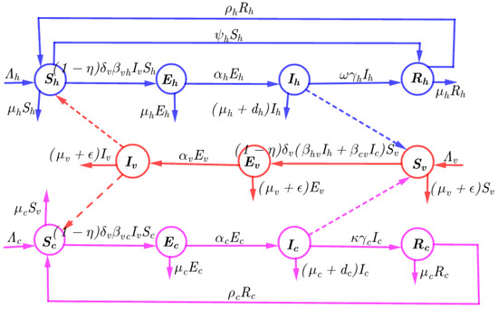
Figure 1.
Model flow chart illustrating the dynamics of HAT disease.

Table 1.
Description of parameters used in system (4).
3. Model Analysis
3.1. Key Definition of Caputo-Fractional Derivatives
In this part, we introduce the key definition of Caputo-fractional derivatives and related theorems that will be applied in this study, (see, [37,38,39,40]) that we will utilize to derive important results in this work.
Definition 1.
Let Caputo-fractional derivative is defined as follows:
Definition 2.
(Constant function related to Caputo fraction calculus [40]). The constant function related to Caputo-fractional derivative is zero, as given below:
Definition 3.
The Liouvile fractional-order derivatives in Caputo sense is stated as follows:
where by is defined as: .
Definition 4.
The integral function of order in Caputo sense is given by:
where by .
3.2. Existence and Uniqueness of Solution
In this section, we examine and study the existence of steady states of model (4) by applying fixed-point theorem techniques. We start by defining the Banach space functions equipped with norm, defined as follows:
where:
It follows that we use the concept presented in (8) and apply the integral derivatives in (4):
which implies that, for , we have the following:
where:
The function related to kernels with satisfies the Lipschitz criterion in (11) provided that and is bounded above. In-general, suppose and are two functions, then:
where . Thus:
Applying the same techniques as in (12), we obtain the following:
with define the constant function related to Lipschitz criterion. Therefore, the system (10) can be defined in recursive form:
Let , be the recursive functions for humans and cattle in (15), then we have the following:
Similarly, for the vector population,
Considering that
and
then applying norm on both sides and using Equations (15) and (16), we have the following:
Theorem 1.
3.3. Numerical Scheme for Model (4) in Caputo Sense
In this section, we investigate the numerical scheme of model (4) in Caputo sense as used in Ghanbari [21]. For the human and the cattle population, the model Equation (22) can be presented as follows:
Similarly, the proposed model differential equation for the vector population can be presented in the Equation (23)
In what follows, we present the Equation (22) for which obeys the Lipschitz criterion given the initial condition . Using the concept of integral in (23), we can have Equation (24)
Let denote the fractional-order derivative in the Caputo sense. Consider the interval with a uniform step size , where . Define as the numerical approximation of at time , where and . Applying the method described in (24), we obtain Equation (25) using the Caputo derivative expression:
where
Theorem 2.
The numerical scheme in (25) is stable.
Proof.
Suppose and approximate and From Equation (25),
Using Equation (25) in (26), we obtain the following:
Using the techniques of Lipschitz criterion and triangular relations, one obtains the following:
where . The expression in (28) can be modified as follows:
where Finally, we have that , and this complete the proof. □
4. Basic Properties
In this part, the basic properties of the model is investigated, we investigate existence of solution for the proposed model.
4.1. Positivity of Solutions
To investigate the behavior of solutions, we state and prove the following theorem:
Theorem 3.
Let: , , , , , , ,
, and for , , is the Cauchy optimal value for the system . Then, for all , , .
Proof.
Let , , , , , , , , , . By continuity of functions and , one can see that . Let . Next, we have to show that . Suppose , then one has that and are non-negative on . At , the following conditions satisfies , , , , , , , , and . Consider the infected class of cattle :
Applying the concept of integral in (30) with the limit 0 to , one obtains the following:
Furthermore, we use the same concept for other equations and we have that , , , and . The results oppose the condition that, . Thus, the maximum condition for the solutions of the Cauchy problem associated to system is non-negative and completes the proof. □
4.2. Boundedness of Trajectories
- We have the following result about the boundedness of trajectories of system .
Lemma 1.
Each non-negative solution of system is bounded on .
Proof.
Consider the human populations, and add the first four equations of model system (4) yields the following:
Using the concept of Gronwall Lemma in (31), one can obtain the following:
In what follows, we have that, for every if . This means that and . Applying the same concept, we can obtain which implies that and . Similarly, we can prove that This mean that: and , and this mark the end of proof. □
Corollary 1.
This show that the model solution of system (4) converge to the fixed point and remain stable for .Consider the area:
with:
and:
4.3. Basic Reproduction Number and Existence of Equilibria
This section focuses on determine the basic reproduction number which quantifies the ability of disease to spread in the population. We use the popular technique known as next generation method to obtain the value of . First of all, we obtain the disease free equilibrium of the model (4) denoted by and given as follows:
Applying the same techniques used in Driessche [41] and Die [42], we define the positive matrix which represents the new infections in the population and matrix denotes the non-singular matrix for representation of disease transfer are defined in (38) and (39): evaluated at the point are defined in (38) and (39):
Suppose and are Jacobian matrix of (38) and (39) evaluated at the disease free equilibrium point , then we have the following:
In what follows, we compute the value of and and the results are presented in (40) and (41):
with , , , , , , , , , , . The eigenvalues correspond to matrix in (41) is denoted by as defined below:
Thus, from (42) one can observe that the for the model (4) is:
with and
The threshold quantity is the expected number of secondary cases produced in a completely susceptible population, by one infected individual during its lifetime as infectious. The square root here is due to the fact that the generation of infection in vector-borne diseases require two transmission processes. Therefore, is the disease transmission from interaction between human and vector populations; is the disease transmission from interaction between cattle and vector population.
Theorem 4.
The system (4) has a disease free equilibrium which is globally asymptotically stable in Ω when and unstable when .
Proof.
If we consider the infected class in (4), we can have the following expression:
where , with F and V defined as follows:
and
This show that is positive and using the concept stated in Perron–Frobenius theorem [43] implies that has non-negative left eigenvectors corresponding to thus,
Since has non-negative vector, for global stability, we consider the following Lyapunov function:
Applying the concept of derivatives in , one obtains the following:
This implies that the optimal invariant subset of where is a point . Thus, applying the concept of LaSalle’s invariance principle stated in [44], is globally asymptotically stable in when . □
5. Results and Discussion
This part present details of numerical simulations of the model, simulated using Euler and Adam–Bashforth–Moulton techniques. Despite the fact that Euler method is effective for numerical simulation, higher-order methods may be necessary for capturing the more subtle dynamics induced by fractional-order derivatives. The numerical results obtained shed light on the impact of proposed control strategies and fractional order derivatives. We start by setting the initial conditions of variables, as , , , , , , , , , , and . Some of the model’s parameters were fitted using real-case data to make the model more realistic, as shown in the Table 2. For simulation purposes and model validation, we choose the value of fractional order derivatives between 0 and 1, and was set to be and . The selection of fractional order between 0 and 1 is based on the fact that as the order of derivative approaches 0, biological species retain its memory for long time and loose easily when the order of derivative approach 1.
Table 2.
Description of parameters used in system (4).
5.1. Model Validation
To ensure the accuracy and realistic of the studied model, we used the real data of HAT cases in Tanzania to validate the model. Parameters for our numerical results were drawn from the literature, and some were calculated to minimize the root-mean-square error (RMSE) as presented in (46).
with n denotes the number of HAT real data reported in Tanzania. We assumed the initial population as follows: , , , , , , , , , , and In addition, from the model (4), the generated new cases are obtained using the term , which counts for the detected cases.
Figure 2 denotes the HAT disease reported real data for 28 years in Tanzania, and the numerical simulations presented in (Figure 3) illustrate that calibration of model at is related to reported cases of HAT disease infections, as shown in Figure 3a. From numerical results, we observe the system (4) has more accurate in restated to the real data of HAT disease cases presented in Table 2. Figure 3b demonstrated the calibration of integer model using HAT disease cases to compare the effectiveness of integer and fractional-order model in disease dynamics. Overall, the results show that fractional-order model had a good fit compared to integer-order model.
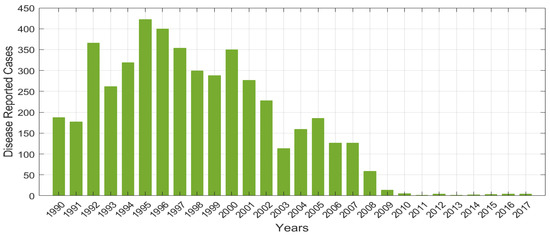
Figure 2.
Number of reported HAT disease cases over 28 years in Tanzania as in the WHO Report [32].
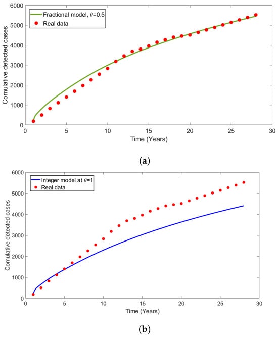
Figure 3.
(a) Fractional model fit versus HAT-reported cases at order of derivative . (b) Model fit versus reported HAT cases at to compare the results of classical integer model with fractional fitted in (a). We used the real data of HAT as in WHO Report [32].
Figure 4 shows the deviation of the estimated parameter values from the given base values. Considering cummulative sum of the square errors depicted by Figure 4, it seems that the sum of the square errors is normally distributed implying goodness of fit for the estimated values on the model (4).
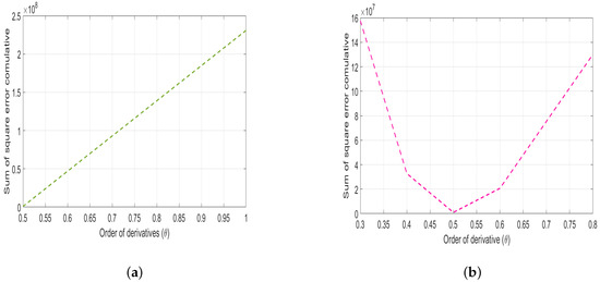
Figure 4.
Plot of the cumulative sum of squared errors (SSER) versus the order of derivatives, with (a) a ranging from 0.5 to 1 and (b) ranging from 0.3 to 0.8.
In (Figure 5), we conducted the model validation through fitting the model with real cases of HAT reported in Tanzania. The correspondence residual is plotted as shown in Figure 5b. The numerical results indicated no significant auto-correlation or partial auto-correlation in the residuals. Furthermore, to assess the applicability of model across the region specifically in East Africa, we fitted the model with HAT cases in Uganda and the corresponding residual is plotted as shown in Figure 6. Overall, one can note that the results obtained in (Figure 6) concur to the results obtained in Figure 3. Implying that the model (Figure 1) is epidemiologically well-formulated and had good fit results to the real data of HAT disease. Thus, the model can be used to study and predict the dynamics of HAT disease in East Africa.
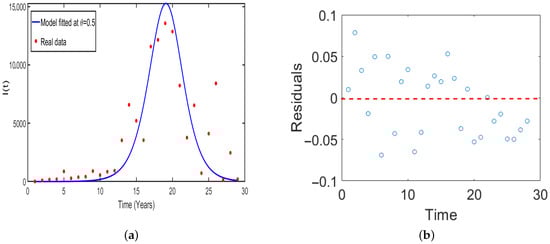
Figure 5.
Plot of (a) Model fitted to the real data of HAT cases against the infected compartment of humans (b) time series against residuals.
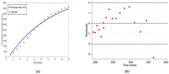
Figure 6.
Plot of (a) Model fit to the reported cases of HAT in Uganda (b) time series against residuals.
5.2. Sensitivity Analysis
This section presents detail of global sensitivity analysis of the studied model using Partial Rank Correlation Coefficient (PRCC). The aim is to investigate relation between model parameters and . Overall, we have noted parameters such as recruitment of human, cattle and vectors (, and ), force of infections (, , and ), vector biting rate (), have positively correlated with . In contrast, the results indicated that, parameters such as use of the insecticides (), rate of the human awareness (), treatment of the infected humans (), vector mortality rate (), have negative indices with . The results show that parameters such as insecticide use and vector mortality rate have the significant in reducing the spread of HAT disease. Therefore, integrating strong control strategies such pyrethroid insecticides and insecticide-treated materials (like targets, treated cattle, indoor residual sprays, and treated nets) are crucial in reducing tsetse fly population in areas affected by HAT. This effectively disrupts the interaction between tsetse flies and their hosts (humans and animals).
Figure 7 shows the correlation of parameters in relation to . From this figure, it can be observed that the rate of tsetse biting rate on the humans and cattle populations , the level of human aware on the HAT disease , and frequency use of insecticide are the most sensitive parameters in this model.

Figure 7.
Sensitivity analysis of (a) to the model parameters that influence the disease transmission between cattle and tsetse flies, (b) to the model parameters that influence the disease transmission between human and tsetse flies.
Numerical results in (Figure 8) demonstrates the influence of key parameters on the disease transmission. It is observed that parameters such as insecticides, and prevention measures when whenever increased number of infected human in decreases. On the other hand, we observed that, an increase in vector biting and the recruitment of tsetse flies in the population lead to an increase in the number infected humans. In particular, one can observe that as the rate of insecticides () and the vector mortality rate () go above , the number of infected humans dies in the population.
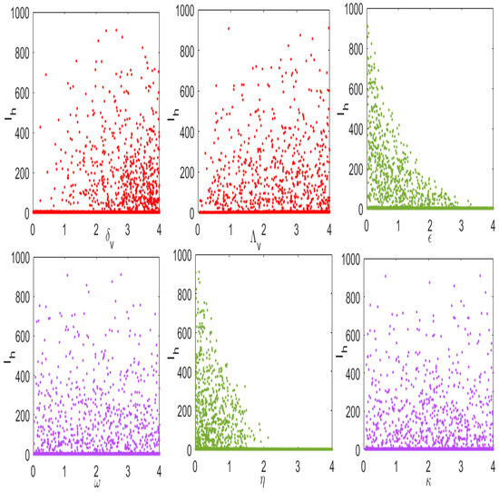
Figure 8.
Numerical results of model (4) in relation infected humans () and parameters with high influence on disease transmission.
Numerical simulations in (Figure 9) show the Latin Hypercube sampling of in relation to parameters that has high influence on the disease transmission. Overall, our results demonstrated that model parameters such as rate of the use of insecticides , prevention measures , and the tsetse deaths have negative correlation with . The results imply to reduce the spread of HAT in community, policy makers and other stakeholders must allocate enough resources for the use of insecticides and prevention measures.
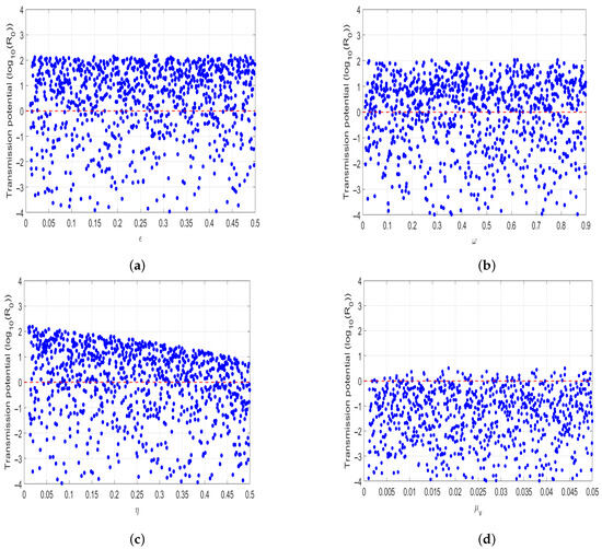
Figure 9.
Numerical Numerical simulation of: (a) Latin Hypercube sampling of and use of insecticides to reduce the vector population, (b) Latin Hypercube sampling of and treatment rate of infected humans, (c) Latin Hypercube sampling of and use of human protective in contact with tsetse flies, (d) Latin Hypercube sampling of and tsetse mortality rate.
Figure 10 is contour simulation of (a) as function of and (health education campaigns). Our results showed that applying both insecticide use and human awareness campaigns, the spread of disease decreases in the population. This imply that policy markers must implement on the use of insecticides to eliminate HAT in the population. Figure 10b shows the contour plot of as a function of (use of insecticides) and (prevention measures). We observed that when the insecticides and prevention measures implemented simultaneously, the HAT disease is easily eliminated in the population. This results demonstrate that policymakers must put effort on use of insecticides and emphasize people to consider wearing long sleeves clothes when visiting tsetse fly infected areas.
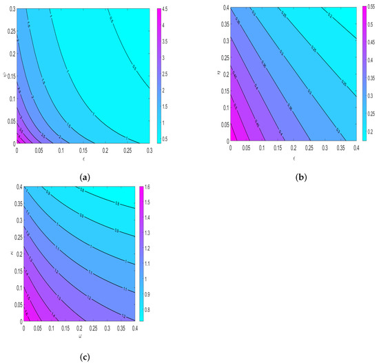
Figure 10.
Numerical simulation of (a) To demonstrate the effects of insecticides () and human awareness (b) To investigate the impact of insecticides () and prevention measures () (c) To assess the effect of treatment of infected human () and cattle ().
5.3. Effect of Memory on the Disease Transmission
In this study, the effect memory (order of derivatives) on HAT transmission is investigated, and we perform the numerical simulation of system (4) for both and and the results is presented in (Figure 11 and Figure 12). For the simulation purposes, memory effects are selected between 0 and 1 and was set to be: (), as mentioned in the literature that when the order of derivatives the fractional-order model based on Caputo derivative becomes a classical ordinary differential model. From the numerical simulations, the results showed that as is close to 0, the memory effects of biological species increase, and numerical results decrease and converges to disease equilibrium, specifically, when the numerical results converges to unique point after 20 days. In contrast, when , the numerical results converges to endemic equilibrium. Additionally, the numerical results demonstrated that as order of derivatives close to 0, the model results converge to equilibrium points earlier than when close to unit.
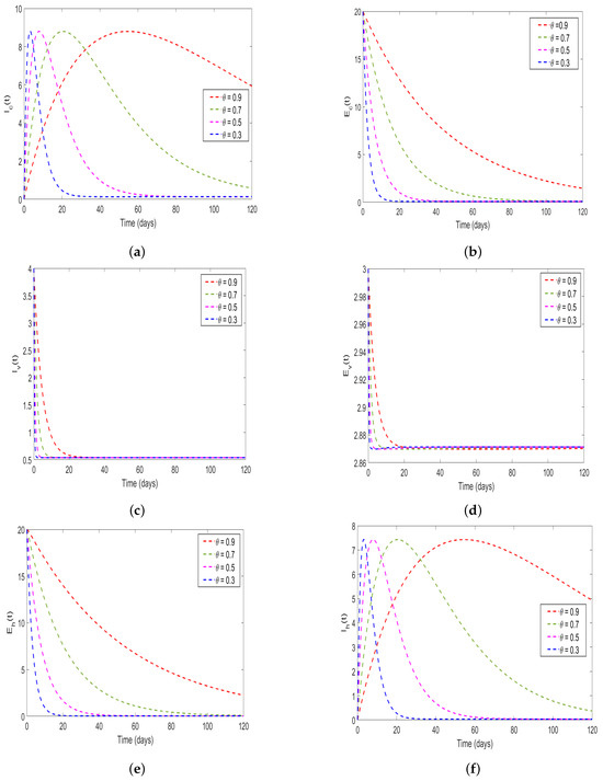
Figure 11.
Numerical results of model (4) at with order of derivatives set to (a) describing the solution behavior of infected cattle, (b) describing the solution behavior of exposed cattle, (c) describing the solution behavior of infected tsetse flies, (d) describing the solution behavior of exposed tsetse flies, (e) describing the solution behavior of exposed humans, (f) describing the solution behavior of infected humans.
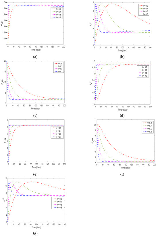
Figure 12.
Simulation solutions of model system 4 at with : (a) describing the solution behavior of recovered humans, (b) describing the solution behavior of infected cattle, (c) describing the solution behavior of exposed cattle, (d) describing the solution behavior of infected tsetse flies, (e) describing the solution behavior of exposed tsetse flies, (f) describing the solution behavior of exposed humans, (g) describing the solution behavior of infected humans. Simulations were carried out using the parameter values shown in Table 2.
5.4. Impact of Insecticides Use on HAT Transmission
The results in (Figure 13) reveals the potential impact of insecticides on reducing the HAT transmission in the population, depicted in bar graphs. Specifically, the result shows implementing insecticides by leads to high reduction in HAT transmission. In this part, Furthermore, we performed the numerical simulations to investigate the effect of insecticides on HAT transmission, and the results are shown in (Figure 14). The numerical results show that effective use of insecticides may lead to decrease the spread disease. Specifically, we observed that as the use of insecticides , the disease remaining endemic in the population. On the other hand, the results demonstrated that as , the disease become eliminated in the population.
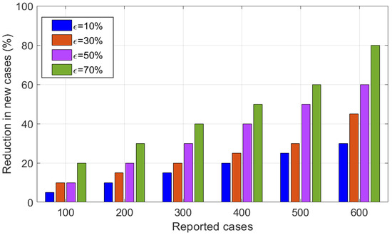
Figure 13.
Impact of insecticides on reduction in disease transmission.
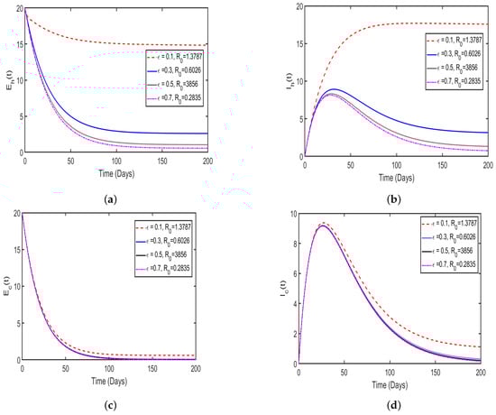
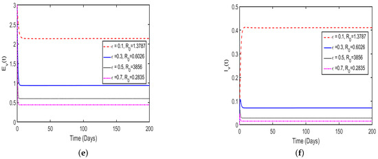
Figure 14.
Numerical results of model system (4) to assess the impact of insecticide on reduce the HAT transmission: (a) from exposed humans to susceptible tsetse flies, (b) from infected humans to susceptible tsetse flies, (c) from exposed cattle to susceptible tsetse flies, (d) from infected cattle to susceptible tsetse flies, (e) from exposed tsetse flies to susceptible human and cattle, (f) from infected tsetse flies to susceptible human and cattle.
Numerical simulations in Figure 9 shows the Latin Hypercube sampling of to model parameter that have high influence on HAT transmission. Overall, the result reveals that model parameters such as insecticides , prevention measures and tsetse mortality rates have negative correlation with . The results imply to eliminate HAT disease in population, policymakers, and other stakeholder need to allocate enough resources on insecticides and prevention mechanism.
5.5. Impact of Prevention Measures on the Disease Dynamics
Numerical results in (Figure 15), shows the simulation of model (4) to assess the impact of prevention measures () on HAT dynamics. Effectiveness of prevention measures can be quantified through use of techniques, such as wearing of long-sleeved and neutral clothes, and use of skin lubricants. to assess the impact of prevention measures, we simulate the model (4) at , , and to show the impact of control on HAT transmission. We observed that as , the disease decreases in the community. Furthermore, we observe that as prevention measures become above , the magnitude of transmission potential () is reduced to less than 1. Next, we investigated the impact of prevention measures on reduce the HAT transmission and the numerical results is shown in (Figure 16). Overall, the results showed that effective use of prevention measures by leads high reduction in HAT transmission.
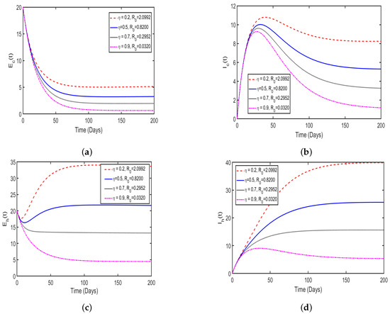
Figure 15.
Model simulation in (4) shows the impact of prevention on HAT transmission: (a) from exposed cattle to susceptible tsetse flies, (b) from infected cattle to susceptible tsetse flies, (c) from exposed humans to susceptible tsetse flies, (d) from infected humans to susceptible tsetse flies.

Figure 16.
Effects of varying on reduction in new HAT cases generated in the population.
Numerical simulations in (Figure 17) show the effects of human awareness campaign () on HAT transmission. Effectiveness use of human awareness campaigns can be applied through use of media platforms including newspapers, television, and social media to inform the public on how to prevent themselves contact with tsetse flies. Therefore, we simulate the model (4) at , and to assess the impact of human awareness on HAT transmission. Overall, the results reveal that use of human awareness alone the size of () can not be less than 1. Thus, the HAT disease cannot be eliminated in the community.
Figure 17.
Simulation of model (4) to investigate the impact of Human awareness on HAT transmission: (a) from exposed humans to susceptible tsetse flies, (b) from infected humans to susceptible tsetse flies, (c) from infected tsetse flies to susceptible humans flies.
5.6. Impact of Human Awareness on HAT Transmission
Figure 17 shows that the increase in health education about spread of HAT among human population by leads to the decline in the rate of susceptibility of human beings by . Consequently, this leads to the decline in the rate of exposure to the disease by throughout the entire simulation period.
6. Concluding Remarks
This study develops a fractional-order model for HAT dynamics, capturing the interplay between human, cattle, and tsetse fly populations. By leveraging Caputo-fractional calculus, the model accounts for memory effects, offering a more realistic representation of HAT dynamics compared to traditional integer-order models. The model, formulated in Section 2, includes key biological aspects, such as susceptible, exposed, infectious, and recovered compartments for humans and cattle, and susceptible, exposed, and infectious compartments for tsetse flies. Key control measures, like, use of insecticides (), prevention strategies (), and human awareness campaigns () are incorporated to assess their impact on disease spread. Analytical results in Section 3 confirm the model’s robustness, and stability. The existence and uniqueness of solutions were established using fixed-point theorems, while positivity and boundedness ensure biological feasibility. The basic reproduction number, , derived via the next-generation matrix method, quantifies disease transmission potential, with contributions from human–vector () and cattle–vector () interactions. Sensitivity analysis using the PRCC reveals that parameters like tsetse biting rate () and recruitment rates (, , ) increase , while insecticides, prevention measures, and human awareness reduce it. When , the free equilibrium point is stable, imply potential for disease elimination with effective interventions.
Numerical simulations, conducted using Euler and Adams–Bashforth–Moulton schemes, our findings. The model was fitted to 28 years of HAT case data from Tanzania (Figure 2), showing that the fractional-order model () outperforms the integer-order model () in capturing reported cases. This highlights the importance of memory effects in modeling chronic diseases like HAT. Simulations varying the fractional order () demonstrate that lower values improve the memory effects, leading to faster convergence to disease-free or endemic equilibria when or , respectively (Figure 11 and Figure 12). The impact of control strategies is significant. Insecticide use at reduces below unity, substantially decreasing new infections (Figure 13 and Figure 14). Prevention measures, such as protective clothing, at , similarly curb transmission (Figure 15 and Figure 16). Combining these measures improves efficacy, with contour plots suggesting that 30% insecticide coverage and robust prevention can eliminate HAT. Health education campaigns, while reducing susceptibility by 97% and exposure by 88% at 78% implementation (Figure 17), are insufficient alone to drive , necessitating integrated approaches.
Despite our model and study’s strengths, the model has limitations. It assumes constant parameters, neglecting seasonality in tsetse fly populations or biting rates, which could influence transmission dynamics. Additionally, since the vector-borne diseases are sensitive to climatic change and life span of vector is short, the effects of seasonality and time delays in tsetse mortality are not considered. In future work, we will incorporate these factors, alongside exploring novel interventions like vaccines, to improve model world applicability. The fractional-order framework provides a versatile tool for modeling other vector-borne diseases, supporting global efforts toward HAT elimination by 2030. Policymakers should prioritize resource allocation for insecticide use and prevention measures, ensuring at least 30% and 50% coverage, respectively, to achieve significant reductions in HAT prevalence.
Author Contributions
Conceptualization, O.K., M.M. and M.H.; methodology, M.M. and M.M.; software, M.H.; validation, O.K., M.M. and M.H.; formal analysis, O.K.; investigation, O.K. and M.H.; resources, A.M.; data curation, M.H. and M.M.; writing—original draft preparation, O.K.; writing—review and editing, O.K., M.M., M.H. and A.M.; visualization, M.H. and O.K.; supervision, M.M. and M.H.; project administration, M.H. and A.M.; funding acquisition, A.M. All authors have read and agreed to the published version of the manuscript.
Funding
This research received no external funding.
Data Availability Statement
The original contributions presented in this study are included in the article. Further inquiries can be directed to the corresponding authors.
Conflicts of Interest
The authors declare no conflicts of interest.
References
- Stich, A.; Abel, P.M.; Krishna, S. Human African trypanosomiasis. BMJ 2002, 325, 203–206. [Google Scholar] [CrossRef]
- Pépin, J. Sleeping sickness: Time for dreaming. Lancet Infect. Dis. 2023, 23, 387–388. [Google Scholar] [CrossRef]
- Helikumi, M.; Mushayabasa, S. Mathematical modeling of trypanosomiasis control strategies in communities where human, cattle and wildlife interact. Anim. Dis. 2023, 3, 25. [Google Scholar] [CrossRef]
- Liana, Y.A.; Shaban, N.; Mlay, G.; Phibert, A. African trypanosomiasis dynamics: Modelling the effects of treatment, education, and vector trapping. Int. J. Math. Math. Sci. 2020, 2020, 8859238. [Google Scholar] [CrossRef]
- Rock, K.S.; Stone, C.M.; Hastings, I.M.; Keeling, M.J.; Torr, S.J.; Chitnis, N. Mathematical models of human African trypanosomiasis epidemiology. Adv. Parasitol. 2015, 87, 53–133. [Google Scholar] [CrossRef]
- Onuorah, M.O.; Namwanje, N.; Baba, A.M. Optimal control model of human African trypanosomiasis. World Sci. News 2023, 178, 136–153. [Google Scholar]
- Gervas, H.E.; Opoku, N.K.-D.O.; Ibrahim, S. Mathematical modelling of human African trypanosomiasis using control measures. Comput. Math. Methods Med. 2018, 2018, 3503514. [Google Scholar] [CrossRef]
- Fèvre, E.M.; Wissmann, B.V.; Welburn, S.C.; Lutumba, P. The burden of human African trypanosomiasis. PLoS Negl. Trop. Dis. 2008, 2, e333. [Google Scholar] [CrossRef] [PubMed]
- Dickie, E.A.; Giordani, F.; Gould, M.K.; Mäser, P.; Burri, C.; Mottram, J.C.; Rao, S.P.S.; Barrett, M.P. New drugs for human African trypanosomiasis: A twenty-first century success story. Trop. Med. Infect. Dis. 2020, 5, 29. [Google Scholar] [CrossRef]
- Martcheva, M. An Introduction to Mathematical Epidemiology; Springer: Berlin/Heidelberg, Germany, 2015; Volume 61. [Google Scholar] [CrossRef]
- Rogers, D.J. A general model for the African trypanosomiases. Parasitology 1988, 97, 193–212. [Google Scholar] [CrossRef] [PubMed]
- Zhang, X.; Liu, X. Backward bifurcation of an epidemic model with saturated treatment function. J. Math. Anal. Appl. 2008, 348, 433–443. [Google Scholar] [CrossRef]
- Ozair, M.; Lashari, A.A.; Jung, I.H.; Okosun, K.O. Stability analysis and optimal control of a vector-borne disease with nonlinear incidence. Discrete Dyn. Nat. Soc. 2012, 2012, 475463. [Google Scholar] [CrossRef]
- Helikumi, M.; Eustace, G.; Mushayabasa, S. Dynamics of a fractional-order chikungunya model with asymptomatic infectious class. Comput. Math. Methods Med. 2022, 2022, 5118382. [Google Scholar] [CrossRef] [PubMed]
- Helikumi, M.; Lolika, P.O. Global dynamics of fractional-order model for malaria disease transmission. Asian Res. J. Math. 2022, 18, 82–110. [Google Scholar] [CrossRef]
- Kouidere, A.; El Bhih, A.; Minifi, I.; Balatif, O.; Adnaoui, K. Optimal control problem for mathematical modeling of Zika virus transmission using fractional order derivatives. Front. Appl. Math. Stat. 2024, 10, 1376507. [Google Scholar] [CrossRef]
- Ali, A.; Iqbal, Q.; Asamoah, J.K.K.; Islam, S. Mathematical modeling for the transmission potential of Zika virus with optimal control strategies. Eur. Phys. J. Plus 2022, 137, 146. [Google Scholar] [CrossRef]
- Rakkiyappan, R.; Latha, V.P.; Rihan, F.A. A fractional-order model for Zika virus infection with multiple delays. Complexity 2019, 2019, 4178073. [Google Scholar] [CrossRef]
- Ullah, M.S.; Higazy, M.; Kabir, K.M.A. Modeling the epidemic control measures in overcoming COVID-19 outbreaks: A fractional-order derivative approach. Chaos Solitons Fractals 2022, 155, 111636. [Google Scholar] [CrossRef]
- Lusekelo, E.; Helikumi, M.; Kuznetsov, D.; Mushayabasa, S. Dynamic modelling and optimal control analysis of a fractional order chikungunya disease model with temperature effects. Results Control Optim. 2023, 10, 100206. [Google Scholar] [CrossRef]
- Ghanbari, B.; Atangana, A. A new application of fractional Atangana–Baleanu derivatives: Designing ABC-fractional masks in image processing. Phys. A 2020, 542, 123516. [Google Scholar] [CrossRef]
- Sharma, N.; Singh, R.; Singh, J.; Castillo, O. Modeling assumptions, optimal control strategies and mitigation through vaccination to Zika virus. Chaos Solitons Fractals 2021, 150, 111137. [Google Scholar] [CrossRef]
- Prasad, R.; Kumar, K.; Dohare, R. Caputo fractional order derivative model of Zika virus transmission dynamics. J. Math. Comput. Sci. 2023, 28, 145–157. [Google Scholar] [CrossRef]
- Mouaouine, A.; Boukhouima, A.; Hattaf, K.; Yousfi, N. A fractional order SIR epidemic model with nonlinear incidence rate. Adv. Differ. Equ. 2018, 2018, 160. [Google Scholar] [CrossRef]
- Rihan, A.F.; Al-Mdallal, M.Q.; AlSakaji, J.H.; Hashish, A. A fractional-order epidemic model with time-delay and nonlinear incidence rate. Chaos Solitons Fractals 2019, 126, 97–105. [Google Scholar] [CrossRef]
- Hamdan, N.I.; Kılıçman, A. Analysis of the fractional order dengue transmission model: A case study in Malaysia. Adv. Differ. Equ. 2019, 2019, 3. [Google Scholar] [CrossRef]
- Helikumi, M.; Ojija, F.; Mhlanga, A. Dynamical analysis of Mpox disease with environmental effects. Fractal Fract. 2025, 9, 356. [Google Scholar] [CrossRef]
- Aksoy, S.; Büscher, P.; Lehane, M.; van den Abbeele, J. Human African trypanosomiasis control: Achievements and challenges. PLoS Negl. Trop. Dis. 2017, 11, e0005454. [Google Scholar] [CrossRef]
- Simo, G.; Rayaisse, J.B. Challenges facing the elimination of sleeping sickness in West and Central Africa: Sustainable control of animal trypanosomiasis as an indispensable approach to achieve the goal. Parasites Vectors 2015, 8, 640. [Google Scholar] [CrossRef]
- Hargrove, J.W.; Ouifki, R.; Kajunguri, D.; Vale, G.A.; Torr, S.J. Modeling the control of trypanosomiasis using trypanocides or insecticide-treated livestock. PLoS Negl. Trop. Dis. 2012, 6, e1615. [Google Scholar] [CrossRef] [PubMed]
- Wamwiri, F.N.; Changasi, R.E. Tsetse flies (Glossina) as vectors of human African trypanosomiasis: A review. Biomed Res. Int. 2016, 2016, 6201350. [Google Scholar] [CrossRef] [PubMed]
- World Health Organization. Report of the Second WHO Stakeholders Meeting on Rhodesiense Human African Trypanosomiasis, Geneva, Switzerland, 26–28 April 2017; World Health Organization: Geneva, Switzerland, 2017. [Google Scholar]
- Franco, J.R.; Simarro, P.P.; Diarra, A.; Jannin, J.G. Epidemiology of human African trypanosomiasis. Clin. Epidemiol. 2014, 6, 257–275. [Google Scholar] [CrossRef]
- Helikumi, M.; Kgosimore, M.; Kuznetsov, D.; Mushayabasa, S. Dynamical and optimal control analysis of a seasonal Trypanosoma brucei rhodesiense model. AIMS Math. 2020, 5, 6928–6948. [Google Scholar] [CrossRef] [PubMed]
- Bonnet, J.; Boudot, C.; Courtioux, B. Overview of the diagnostic methods used in the field for human African trypanosomiasis: What could change in the next years? Biomed Res. Int. 2015, 2015, 583262. [Google Scholar] [CrossRef]
- Özköse, F.; Yılmaz, S.; Şenel, M.T.; Yavuz, M.; Townley, S.; Sarıkaya, M.D. A mathematical modeling of patient-derived lung cancer stem cells with fractional-order derivative. Phys. Scr. 2024, 99, 115235. [Google Scholar] [CrossRef]
- Vargas-De-León, C. Volterra-type Lyapunov functions for fractional-order epidemic systems. Commun. Nonlinear Sci. Numer. Simul. 2015, 24, 75–85. [Google Scholar] [CrossRef]
- Caputo, M. Linear models of dissipation whose Q is almost frequency independent, Part II. Geophys. J. R. Astr. Soc. 1967, 13, 529–539, reprinted in Fract. Calc. Appl. Anal. 2008, 11, 4–14. [Google Scholar] [CrossRef]
- Diethelm, K. The Analysis of Fractional Differential Equations: An Application-Oriented Exposition Using Differential Operators of Caputo Type; Springer: Berlin/Heidelberg, Germany, 2010. [Google Scholar]
- Podlubny, I. Fractional Differential Equations; Academic Press: San Diego, CA, USA, 1999. [Google Scholar]
- van den Driessche, P.; Watmough, J. Reproduction number and sub-threshold endemic equilibria for compartmental models of disease transmission. Math. Biosci. 2002, 180, 29–48. [Google Scholar] [CrossRef]
- Diekmann, O.; Heesterbeek, J.A.P.; Metz, J.A.J. On the definition and the computation of the basic reproduction ratio R0 in models for infectious diseases in heterogeneous populations. J. Math. Biol. 1990, 28, 365–382. [Google Scholar] [CrossRef]
- Shuai, Z.; Heesterbeek, J.A.P.; van den Driessche, P. Extending the type reproduction number to infectious disease control targeting contact between types. J. Math. Biol. 2013, 67, 1067–1082. [Google Scholar] [CrossRef]
- LaSalle, J.P. The Stability of Dynamical Systems; SIAM: Philadelphia, PA, USA, 1976. [Google Scholar]
- Martin, G.J.; Friedlander, A.M. Bacillus anthracis (anthrax). In Mandell, Douglas, and Bennett’s Principles and Practice of Infectious Diseases, 7th ed.; Mandell, G.L., Bennett, J.E., Dolin, R., Eds.; Churchill Livingstone: Philadelphia, PA, USA, 2010; pp. 2715–2725. [Google Scholar]
- Ndondo, A.M.; Munganga, J.M.W.; Mwambakana, J.N.; Saad-Roy, M.C.; van den Driessche, P.; Walo, O.R. Analysis of a model of gambiense sleeping sickness in human and cattle. J. Biol. Dyn. 2016, 10, 347–365. [Google Scholar] [CrossRef][Green Version]
Disclaimer/Publisher’s Note: The statements, opinions and data contained in all publications are solely those of the individual author(s) and contributor(s) and not of MDPI and/or the editor(s). MDPI and/or the editor(s) disclaim responsibility for any injury to people or property resulting from any ideas, methods, instructions or products referred to in the content. |
© 2025 by the authors. Licensee MDPI, Basel, Switzerland. This article is an open access article distributed under the terms and conditions of the Creative Commons Attribution (CC BY) license (https://creativecommons.org/licenses/by/4.0/).