Article

The General Semimartingale Market Model

1
Faculty of Economic Studies, University of Finance and Administration, 10100 Prague, Czech Republic
2
Department of Mathematical Sciences, University of South Africa, Florida 0003, South Africa
AppliedMath 2025, 5(3), 97; https://doi.org/10.3390/appliedmath5030097 (registering DOI)
Submission received: 25 May 2025 / Revised: 15 July 2025 / Accepted: 17 July 2025 / Published: 1 August 2025

Abstract

This paper develops a unified framework for mathematical finance under general semimartingale models that allow for dividend payments, negative asset prices, and unbounded jumps. We present a rigorous approach to the mathematical modeling of financial markets with dividend-paying assets by defining appropriate concepts of numéraires, discounted processes, and self-financing trading strategies. While most of the mathematical results are not new, this unified framework has been missing in the literature. We carefully examine the transition between nominal and discounted price processes and define appropriate notions of admissible strategies that work naturally in both settings. By establishing the equivalence between these models and providing clear conditions for their applicability, we create a mathematical foundation that encompasses a wide range of realistic market scenarios and can serve as a basis for future work on mathematical finance and derivative pricing. We demonstrate the practical relevance of our framework through a comprehensive application to dividend-paying equity markets where the framework naturally handles discrete dividend payments. This application shows that our theoretical framework is not merely abstract but provides the rigorous foundation for pricing derivatives in real-world markets where classical assumptions need extension.

1. Introduction

Mathematical finance began with L.F. Bachelier’s 1900 dissertation “Théorie de la Spéculation” [1]. Bachelier first described Brownian motion as a stochastic process, though he did not use that name. He aimed to derive theoretical values for options on commodities by modeling prices with Brownian motion and comparing these prices with market data. He proposed option prices as the expected value of the option payoff. Bachelier’s model had one major flaw: prices could become negative. After decades of neglect, financial mathematics revived in the 1960s when researchers developed stochastic integration theory and introduced geometric Brownian motion for pricing models [2,3,4,5,6,7].
Fischer Black and Myron Scholes made the field’s major breakthrough in 1973 with their famous equation and formula [8]. This work established financial mathematics as a large research area and led to many new models. The development of stochastic analysis and integration theory by Doob [9], Meyer [10,11], Kunita and Watanabe [12], Meyer [13,14,15,16], Doléans-Dade and Meyer [17], Meyer [18], Jacod [19], Chou et al. [20], and Jacod [21] opened new research directions. In particular, the work by Doléans-Dade and Meyer [17] and Jacod [19], who termed the word “semimartingale” as the most general class of processes for which a meaningful stochastic integral can be defined, provided the mathematical foundation for general asset price models that include both continuous and jump components. Since their introduction in the late 1960s, semimartingales have become the fundamental mathematical framework for modeling financial markets. Further, the Black–Scholes model can be viewed as a special case of semimartingale models, where the price process is a continuous semimartingale.
The emergence of modern option pricing based on the replication principle became important as an application of semimartingale theory and representation theorems. The work of Harrison and Pliska [22] was central to this development, which established that under no-arbitrage conditions, discounted asset prices must be semimartingales.
Despite many different models being studied during this time, no general theory unified these models or provided a foundation for financial market modeling. Important progress in general financial mathematical theory came in the 1990s through Delbaen and Schachermayer [23,24]. They presented a general financial market model based on semimartingales that included almost all known models and proved the connection between arbitrage and mathematical conditions on the existence of specific probability measures. Most publications since then have used this semimartingale model framework.
The financial market model in [24] can be seen as the general market that includes almost all frictionless market models used in practice. This model explicitly uses the semimartingale property as the minimal mathematical requirement for asset price processes to allow for meaningful financial modeling, as emphasized by Jarrow [25] and Bichteler [26]. The results are therefore general, and this market setup is the most important model in mathematical finance. Recent work by Kabanov and Safarian [27] and Fontana [28] has further extended semimartingale models to include market frictions and liquidity considerations. However, several gaps exist in the literature, particularly regarding the extension of semimartingale models to more complex market settings:
  • The model in [24] is formulated in a discounted framework (also referred to as a normalized setting). However, most models used in practice are expressed in non-discounted terms, as this facilitates the verification of model assumptions against real-world data. The question of how, and under which conditions, a non-discounted semimartingale model can be transformed into a discounted one has not been addressed in generality, but only for specific model classes, as noted by Platen and Heath [29].
  • The framework presented in [24] does not account for dividends or other intermediate cash flows. As a result, it excludes important applications, such as models for the pricing and hedging of futures contracts. While dividend-paying assets can still be modeled as semimartingales, the precise conditions under which the semimartingale property is preserved under various transformations need clarification, as discussed in Korn [30] and Rogers and Williams [31]. In many cases, models with dividends can be converted into equivalent models without dividends (see, for instance, [32] (Section 2.3)). Consequently, a generalization of the basic semimartingale model to incorporate dividends is both natural and desirable. The importance of dividend modeling has been demonstrated empirically by Whaley [33], who showed significant pricing errors when dividends are not properly accounted for in American option valuation.
  • Several foundational properties of semimartingale market models are often taken for granted without rigorous validation in this highly general setting. This includes concepts such as admissible strategies, discounted asset processes, and the choice of numéraire.
This paper addresses these specific gaps by (1) providing a rigorous mathematical framework for transforming between nominal and discounted semimartingale models under general conditions, (2) extending the semimartingale framework to incorporate dividend payments while preserving key mathematical properties, and (3) carefully validating foundational concepts like admissible strategies and numéraire choice in this general setting. Our main contribution is the unification of these extensions into a coherent framework that maintains the semimartingale structure throughout.
To make our theoretical framework concrete and demonstrate its practical relevance, we present a comprehensive application to dividend-paying equity markets, showing that our general treatment of dividends naturally encompasses standard equity derivatives while maintaining mathematical rigor. This application validates that our unified framework addresses real market phenomena that cannot be handled by classical models without appropriate extensions. Besides the above-mentioned standard reference [33], numerous studies show that dividend considerations materially affect option prices. For instance, Harvey and Whaley [34] documented that dividend uncertainty significantly impacts S&P 100 index option valuation, while more recent work on dividend derivatives markets (see, e.g., the analysis of Euro Stoxx 50 dividend futures in Wilkens and Wimschulte [35]) demonstrates the importance of proper dividend modeling for modern derivative products.
The paper is organized as follows: Section 2 presents the general semimartingale model with dividends, including the mathematical framework and key definitions. Section 3 discusses fair prices and derivative pricing within this framework. Section 4 presents an application to dividend-paying equity markets, illustrating how the framework handles discrete dividend payments in a standard financial setting. The Appendix A contains referenced technical results. Throughout, we emphasize both mathematical rigor and economic intuition to make the framework accessible to both theorists and practitioners.
To guide readers through the logical structure of our framework, Figure 1 presents a flowchart showing the dependencies between key concepts and results.
This article is a revised and expanded version of a paper titled The General Semimartingale Model with Dividends, which was presented at the 10th Rocník Konference Doktorandů Na Vysoké škole Finanční A Správní in Prague on 15 November 2023 [36].

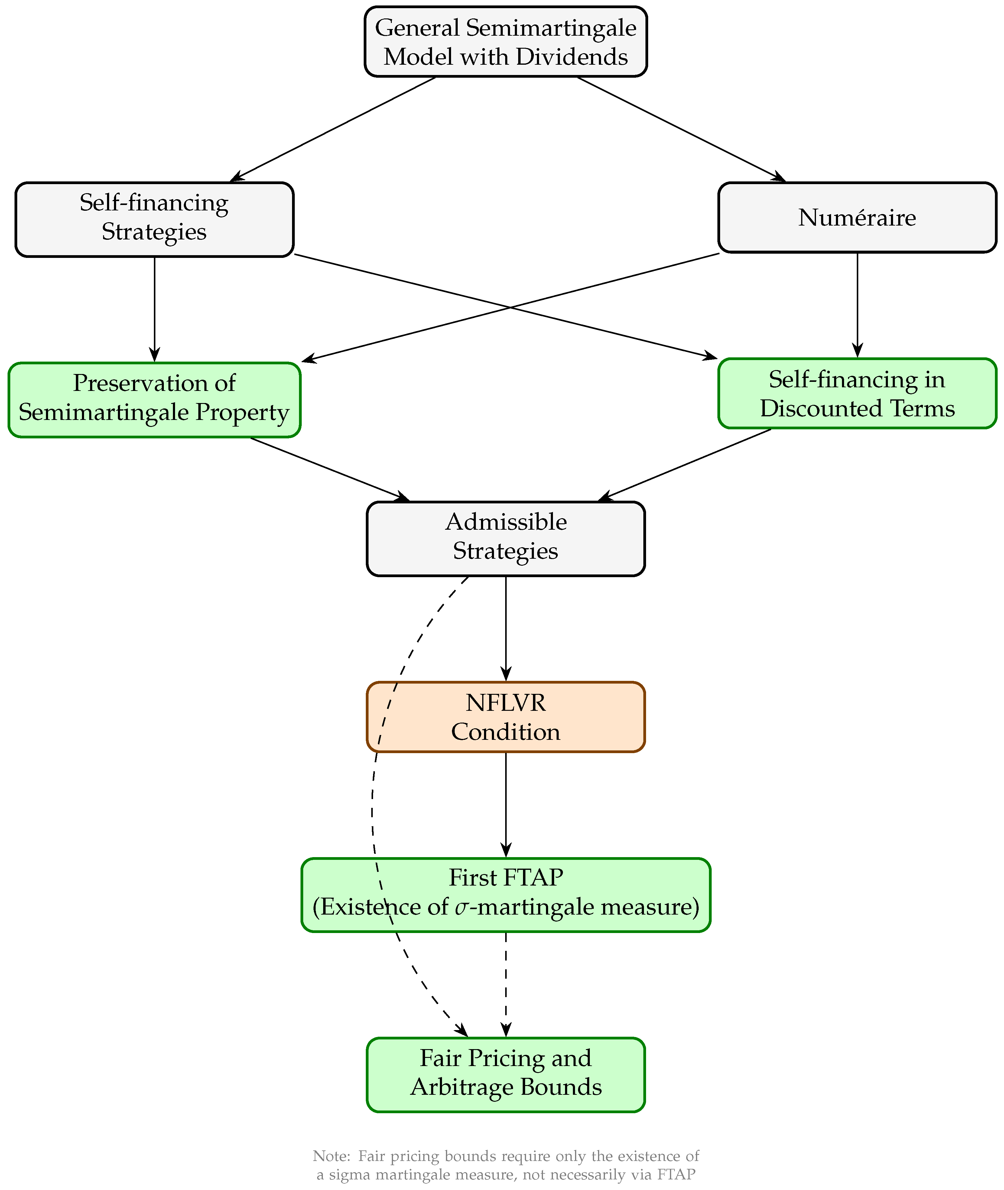
2. The General Semimartingale Model with Dividends

In this section, we establish a general market model that incorporates dividends. We focus on continuous-time models. While discrete models form a special case of continuous-time models and offer simpler mathematical treatment, continuous-time models dominate financial mathematics, particularly in portfolio theory. This is because continuous-time models provide clean, unique solutions to optimization problems while discrete-time models often lack unique solutions and require approximate strategies, which complicates calculations.
Given an R d -valued semimartingale S, we define L ( S ) as the space of integrands for S in general vector-valued stochastic integration with semimartingale integrators. For a semimartingale S, φ L ( S ) , and t R + , we write
φ · S t = φ 0 S 0 + ( 0 , t ] φ d S u
for the stochastic integral at time t. See [37] or [38] for the general vector-valued integral definition.
We study a financial market with d + 1 tradable securities. The price processes follow the d + 1 -dimensional process:
S t = ( S t 0 , S t 1 , , S t d ) t R + .
Each security has an associated cumulative dividend process:
D = ( D t 0 , D t 1 , , D t d ) t R + ,
adapted to the filtration F = ( F t ) t R + .
We begin by discussing the assumptions of frictionless and competitive markets, which are standard in mathematical finance but have important practical implications and limitations.
We assume the market is frictionless and competitive. A frictionless market has no transaction costs, taxes, or trading constraints like short sale restrictions, borrowing limits, or margin requirements. Assets are infinitely divisible. A competitive market means traders act as price takers. Traders can buy or sell any quantity without affecting market prices, eliminating liquidity risk.
While these assumptions simplify the mathematical analysis considerably, they represent idealizations that may not hold in practice. Transaction costs, particularly for high-frequency trading, can be substantial. Market impact is a real concern for large trades, and regulatory constraints often limit trading strategies. However, these assumptions provide a useful baseline model from which more realistic models can be developed by relaxing specific assumptions. For instance, transaction cost models can be viewed as perturbations of the frictionless model, and liquidity constraints can be incorporated through additional state variables or constraints on the strategy space.
Importantly, many of our theoretical results remain valid under small transaction costs. As shown by Guasoni [39] and Kabanov and Stricker [40], when transaction costs are sufficiently small, the fundamental properties of semimartingale models persist, specifically as follows:
  • The semimartingale property of price processes is preserved under small proportional transaction costs.
  • The existence of equivalent sigma martingale measures extends to models with small transaction costs, though the measures must be interpreted in a bid–ask spread context.
  • Self-financing strategies can be generalized to account for transaction costs by modifying the wealth equation to include cost terms.
  • Fair pricing bounds widen to reflect the bid–ask spread, but the fundamental arbitrage relationships remain intact.
While a full treatment of transaction costs is beyond the scope of this paper, we note that our framework provides the foundation upon which transaction cost models can be built. The key insight is that transaction costs can be viewed as a perturbation of the frictionless case, with most qualitative results carrying over when costs are small.
We also assume the following:
  • ( Ω , F , F , P ) is a filtered probability space with probability measure P .
  • The processes S t i and D t i are semimartingales for all i = 0 , , d .
  • The filtration F satisfies the usual conditions and the σ -algebra F 0 is trivial: A F 0 implies P ( A ) = 0 or P ( A ) = 1 .
Remark 1.
Markets with dividends can often become dividend-free through transformation. These transformations require additional assumptions that do not always apply. For example, ref. [32] assumes all cash flows are positive and the numéraire follows a deterministic continuous finite variation process.
The process D t i represents cumulative dividend payments of the i-th share through time t. We do not require monotonicity, so dividend payments can be negative. Non-monotonic dividend processes are important for studying products like futures, where they represent cash flows such as margin payments.
The economic rationale for allowing non-monotonic dividend processes extends beyond futures markets. In practice, negative "dividends" can represent various cash outflows from shareholders, including the following:
  • Capital calls in private equity or venture capital investments;
  • Margin requirements in leveraged positions;
  • Storage costs for commodity investments;
  • Management fees in fund structures;
  • Tax liabilities passed through to investors.
By allowing non-monotonic dividend processes, our framework can model a broader class of financial instruments and investment structures that require periodic cash flows in both directions.
Dividend processes fall into three categories:
First, dividend processes with continuous paths. These are mathematically convenient but unrealistic.
Second, discrete dividend payments, where the dividend process D is a pure jump process ( D = Δ D ) . This matches reality better but is mathematically more complex. Empirical evidence strongly supports this modeling choice. For instance, Mixon [41] demonstrated that using discrete dividend models significantly improves the accuracy of implied volatility extraction from option prices compared to continuous dividend approximations.
Third, any combination of continuous and discrete payments. This is the most general case and the one we use here.
The semimartingale assumption for price processes is mathematically justified because the standard definition of general stochastic integration uses semimartingales as integrators. Economic justification also exists: if the price process is locally bounded and adapted, and the market satisfies ‘No Free Lunch With Vanishing Risk’ (a version of ‘No Arbitrage’), then the price process is a semimartingale. This is shown in [42] (Theorem 8) and [23] (pp. 504–507). Ref. [43] provides another economic argument: in markets with only simple predictable trading strategies, no short-selling, and no-arbitrage, price processes are always semimartingales.
The semimartingale requirement excludes fractional Brownian motions with Hurst parameter H 1 2 . No consistent no-arbitrage theory exists for these processes in frictionless, continuous trading markets. However, in markets with transaction costs, arbitrage opportunities disappear, making fractional Brownian motions reasonable, as in [39].

2.1. Self-Financing Trading Strategies

Definition 1.
(a) 
A d + 1 -dimensional process φ = ( φ 0 , , φ d + 1 ) L ( S ) is called a trading strategy.
(b) 
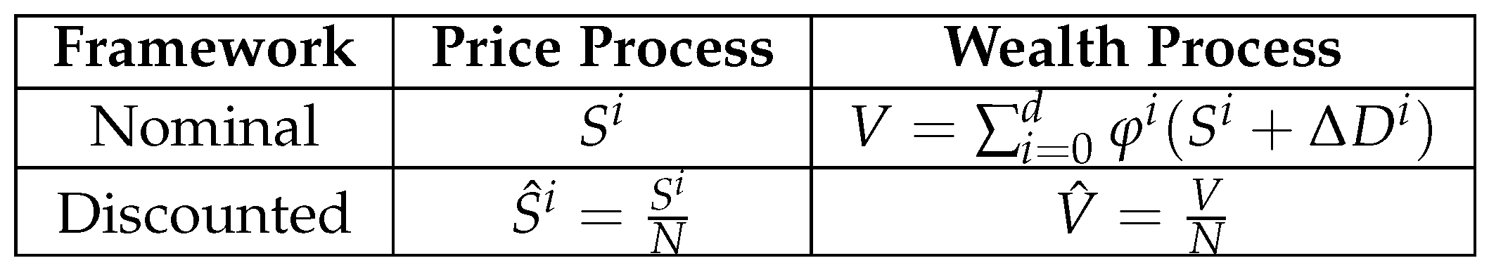
The wealth process of the investor is defined as
V t : = i = 0 d φ t i S t i + Δ D t i , t R + ,
where φ t i represents the number of the i-th security that an investor holds in his portfolio at t.
Definition 2.
A trading strategy φ = ( φ 0 , φ 1 , , φ d ) is called self-financing if the wealth process V t ( φ ) satisfies
V t = φ s · S + D t , for all t R + .
Note (2) deals with higher dimensional processes and hence multi-dimensional integration.
Remark 2.
A trading strategy φ is self-financing if the changes in the associated wealth process V ( φ ) = i = 0 d φ i S i + Δ D i are the result of changes in the price of the assets included. All shifts in the portfolio are cost-neutral and there is no external capital injection or withdrawal. This definition and explanation can be better illustrated by considering time-discrete processes (as a special case of the time-continuous processes).
To keep it simple, we consider only a one-dimensional process in this illustration. In the discrete model, let φ n be the number of securities purchased at price S n 1 (i.e., after the jump S n 1 S n 2 ). Since the dividends accrued in the previous period φ n 1 Δ D n 1 still have to be reinvested, the self-financing condition is
φ n S n 1 = φ n 1 ( S n 1 + Δ D n 1 ) , n = 1 , 2 ,
It can be shown that (3) is equivalent to
φ n ( S n + Δ D n ) = φ n 1 ( S n 1 + Δ D n 1 ) + φ n ( Δ S n + Δ D n ) , n = 1 , 2 ,
Equation (4) is the discrete-time special case of condition (2).
Remark 3.
The variable φ t i denotes the number of securities i that the agent holds in the portfolio during the interval from t to t (in discrete time, from t 1 to t). The jumps Δ S t i and Δ D t i occur simultaneously. We interpret S i as the ex-dividend price, meaning the security price after dividend payment.
At time t, the agent receives dividend payments totaling
i = 0 d φ t i Δ D t i .
These payments are immediately reinvested in the d + 1 securities. No cash is held permanently. This explains why only Δ D and not D appears in Equation (1).

2.2. Numéraire

Comparing asset values at different times using nominal amounts is impractical and meaningless. We need a benchmark to create comparable values. This benchmark is called a numéraire.
Definition 3.
A predictable semimartingale ( N t ) t R + satisfying
inf t [ 0 , T ] N t > 0 , for all T R + P a . s .
is called a numéraire.
Remark 4.
Predictability is required so that 1 N can serve as an integrand. This is needed to define the discounted dividend process and to transfer the self-financing condition from price processes to their discounted versions.
Expressing asset values as multiples of the numéraire allows time-independent comparisons. We denote discounted processes by S ^ i or V ^ :
S ^ i : = S i N and V ^ : = V N .
We need the following result for further analysis.
Lemma 1.
Let N be a numéraire. Then, 1 N is bounded on each compact interval and therefore locally bounded.
Proof. 
By the numéraire definition, inf t [ 0 , T ] N t > 0 a.s. for all T R + . On any compact interval [ a , b ] , there exists δ > 0 such that N t > δ a.s. for all t [ a , b ] . This gives 1 N t < 1 δ a.s. on [ a , b ] . □
The numéraire definition varies across the literature. In [44,45,46], only a positive semimartingale is required. This approach appears in [47], considered the reference for numéraires in abstract settings. However, ensuring discounted price processes remain semimartingales requires the numéraire’s left limit to exceed zero. Some contexts demand stricter conditions, as in [48]. Ref. [49] discusses strong versus weak numéraire concepts. Our definition matches [50]. Recent work describes financial models without numéraires, but this requires more complex market assumptions, as shown in [51], to preserve the ability to discount price processes.
Following (6), we must define both a discounted dividend process D ^ i and a discounted wealth process V ^ . The process D ^ t represents cumulative dividends through time t. Each dividend is discounted by the numéraire value N at its payment time, not at time t. This ensures the discounted dividend process D ^ i changes only when the dividend process D i changes. With an approach like D i N , this property fails because changes in the numéraire N alone would alter D i N .
This leads to the following definition.
Definition 4.
By
D ^ t i : = 1 N · D t i , i = 0 , , d .
the discounted dividend processes is denoted. Furthermore,
V ^ ( φ ) : = V N ( φ ) = i = 0 d φ i ( S ^ i + Δ D ^ i )
denotes the discounted wealth process.
Remark 5.
By Theorem A1, one has Δ D ^ i = Δ D i N .
While it is commonly assumed that D is a pure jump process, we want to avoid making this assumption here and rather stay as general as possible.
However, if we operate under the assumption that the dividend process is a pure jump process (meaning D = Δ D is valid), then, by Theorem A1, we arrive at
D ^ i = 1 N · D t i = 1 N · 0 s t Δ D s i = 0 s t Δ 1 N · D i s = 0 s t Δ D ^ s i .
In this scenario, D ^ also becomes a pure jump process, only changing when D does.
Economically speaking, (7) is logical as it considers the varying times at which increases in D are paid out as dividends. For instance, let us say N = exp ( r t ) and there was just one dividend payment of amount K. Intuitively, a dividend disbursed earlier (at t = 0 ) holds more value than one distributed later (at T = 1 ). If we were to assign the value D ^ i = D i N , the timing of this singular dividend payment would not matter for D ^ . The result would be D ^ 1 = K exp ( r ) . However, with our definition of the discounted dividend process, and by Theorem A1, we get
D ^ 0 = K and D ^ 1 = K exp ( r ) < K .
The next theorem provides the technical foundation for studying properties in discounted settings with standard stochastic analysis tools.
Theorem 1.
The processes N , S 0 , , S d , D 0 , , D d are semimartingales and N is a numéraire if and only if the processes 1 N , S ^ 0 , S ^ d , D ^ 0 , , D ^ d are semimartingales and 1 N is a numéraire. If φ is self-financing, then the discounted wealth process V ^ ( φ ) is a semimartingale.
Proof. 
We provide the key steps of this proof, which demonstrates how the semimartingale property is preserved under the numéraire transformation. The intuition is that the reciprocal of a strictly positive semimartingale remains a semimartingale when properly localized.
“⇒” Assume N is a numéraire and S 0 , , S d are semimartingales.
Define
T n : = inf t 0 ; N t 1 n .
By Equation (5), ( T n ) forms a localizing sequence. Consider the processes
N t n : = ( N n ) t T n : = N t for t < T n , N T n for t T n .
Let f n be a convex function with f n ( x ) = 1 x for x 1 n . By Remark A1, f n ( N n ) is a semimartingale. Since N n 1 n , we have 1 N n is also a semimartingale. Therefore, 1 N n is prelocally a semimartingale and hence, by Theorem A5, a semimartingale.
Since N is a semimartingale and therefore càdlàg, we have
P sup t [ 0 , T ] N t < = 1 for all T R +
which gives
inf t [ 0 , T ] 1 N t > 0 for all T R + P almost surely .
Thus, 1 N is a numéraire and S ^ i = S i N is a semimartingale by Theorem A2.
“⇐” Assume 1 N , S ^ 0 , , S d are semimartingales and 1 N is a numéraire.
Proceeding similarly, we get N = 1 1 N is a semimartingale and, by the same argument, N is càdlàg. Hence, N is a numéraire. Since
S i ^ ^ = S ^ i 1 N = S i i = 0 , d
the processes S i are semimartingales.
For self-financing φ , we have V ^ t = 0 t φ d S u N t , which is a semimartingale by Theorem A2. □
The above theorem establishes a fundamental equivalence: the semimartingale property is preserved when moving between nominal and discounted frameworks. This is crucial for practical applications, as it allows us to work in whichever framework is more convenient for a given problem while maintaining the mathematical structure needed for stochastic integration and arbitrage theory, as is shown by Figure 2.
Most papers tacitly treat nominal models and their discounted counterparts and settings, with or without dividends, as interchangeable: one simply divides by a numéraire or subtracts cumulative dividends and all desired results still hold. In fact, this equivalence is valid for virtually every statement we need in this section.The next theorem, however, shows that a mild additional requirement, namely a specific orthogonality between the numéraire scaled dividend streams and the numéraire itself, is necessary to transfer the self-financing property from the nominal to the discounted world and back.
To state the condition, we recall the decomposition of a semimartingale X = X c + X d into its continuous part X c and its purely discontinuous part X d .
Definition 5.
For two semimartingales X and Y we set
[ X , Y ] t c : = [ X c , Y c ] t , t [ 0 , T ] .
In particular, [ X ] c : = [ X , X ] c .
With the above definition, we get
[ X , Y ] t = [ X , Y ] t c + 0 s t Δ X s Δ Y s .
The following theorem states that the self-financing property stays valid regardless of whether the associated wealth process is viewed in nominal or discounted terms.
Theorem 2.
Let φ = ( φ 0 , φ 1 , , φ d ) be a trading strategy, V be the associated wealth process, and N a numéraire with [ N , D i ] c = 0 for all i { 0 , , d } . Then, φ is self-financing if and only if
V ^ t ( φ ) = i = 0 d φ i · ( S ^ i + D ^ i ) t , t [ 0 , T ] ,
where v ^ 0 : = v 0 N 0
The condition [ N , D i ] c = 0 ensures that the continuous parts of the numéraire and cash flow processes do not covary. This orthogonality condition is necessary for the self-financing property to transfer correctly between nominal and discounted frameworks. While this condition is automatically satisfied when D is a pure jump process (discrete dividends) or when N is deterministic (constant interest rates), it represents a genuine restriction when both processes have stochastic continuous components. In such cases, the condition requires that continuous cash flows are not systematically correlated with continuous changes in the discount factor.
Proof. 
We show the one-dimensional case. The multi-dimensional case follows from the linearity of the integral and the fact that any strategy can be approximated by component-wise integrable strategy.
We have Δ V = φ Δ S and therefore, it is easy to see that
V = φ S and V ^ = φ S ^ .
We first assume
V ^ t ( φ ) = φ · ( S ^ + D ^ ) t .
By Theorem 1, V ^ = V ^ ( φ ) is a semimartingale, and with Theorem A1, we obtain
Δ V ^ = φ Δ ( S ^ + D ^ ) .
By definition, we also have
V ^ = φ ( S ^ + Δ D ^ ) ,
and therefore,
V ^ = V ^ Δ V ^ = φ ( S ^ Δ S ^ ) = φ S ^
With Theorem A4, we obtain
V t = V ^ t N t = N · V ^ t + V ^ · N t + [ N , V ^ ] t = N · φ · ( S ^ + D ^ ) t + φ S ^ · N t + N , φ · ( S ^ + D ^ ) t = φ · N · ( S ^ + D ^ ) + S ^ · N + N , S ^ + D ^ t = φ · N · S ^ + ( N Δ N ) · D ^ + S ^ · N + N , S ^ + N , D ^ t = φ · N · S ^ + S ^ · N + N , S ^ = N S ^ + N · D ^ Δ N Δ D ^ + N , D ^ c = 0 + Δ N Δ D ^ t = φ · N S ^ + N · D ^ t = φ · N S ^ + N · 1 N · D t = φ · ( S + D ) t
Hence, φ is self-financing. The converse follows analogously with N = 1 N and V ^ = V N .
Since each trading strategy can be approximated with component-wise integrable trading strategy, the general result follows by taking limits. □
Definition 6.
Let S = ( S 0 , , S d ) be a d + 1 -dimensional semimartingale, D = ( D 1 , , D d ) a d-dimensional semimartingale, S 0 a numéraire, and Q a probability measure that is equivalent to P .
(a) 
Q is called an equivalent martingale measure if S ^ i + D ^ i : = S i S 0 + 1 S 0 · D i is a Q -martingale for all i { 1 , , d } .
(b) 
Q is called an equivalent local martingale measure if S ^ i + D ^ i is a local Q -martingale for all i { 1 , , d } .
(c) 
Q is called an equivalent sigma martingale measure if S ^ i + D ^ i is a sigma martingale under Q for all i { 1 , , d } .
The distinction between martingales, local martingales, and sigma martingales has important economic implications:
  • Martingales represent fair games where expected future value equals current value. This is the strongest condition and ensures that all trading strategies have bounded expected returns.
  • Local martingales allow for the possibility of asset price bubbles, where prices can temporarily deviate from fundamental values. They are martingales when stopped at appropriate times but may exhibit explosive behavior.
  • Sigma martingales are the weakest condition still sufficient for no-arbitrage. They allow for both bubbles and certain types of market incompleteness while maintaining the essential no-arbitrage property. In mathematical terms, a strict local martingale is a process that essentially has no trend but cannot, not even locally, be integrated (see [52] for more details).
The economic significance is that moving from martingales to sigma martingales allows modeling increasingly realistic market phenomena while preserving the mathematical framework needed for derivative pricing.

2.3. Admissible Strategies

The class of possible trading strategies involves strategies that would be difficult to realize. Therefore, this class should be further restricted and exclude the strategies that would require the investor to have an infinite line of credit with the bank.This also prohibits the so-called duplication strategies, which otherwise offer arbitrage opportunities in most markets, which was already noted by [22].
Definition 7.
A self-financing strategy φ = ( φ 0 , φ 1 , , φ d ) L ( S ) is called admissible, if there exists an α R + , such that one has
V t α for all t [ 0 , )
for the corresponding wealth process V.
By Φ ( S ) , we denote the set of admissible strategies belonging to the price process ( S t ) t R + .

2.3.1. Overview of Admissibility Definitions

The definition of admissibility is not unique in the literature. There are several common definitions. It shall be noted that the models used in the literature given here usually do not consider dividends. However, the definition of admissibility is independent of the dividend process.
A self-financing strategy φ L ( S ) is called admissible, if
(a)
there exist a , b > 0 such that a V ^ t b almost surely [53,54];
(b)
V ^ t is a martingale under an equivalent martingale measure Q for the corresponding wealth process V [55,56,57];
(c)
V ^ ( φ ) is square integrable [45];
(d)
one has V t 0 for the corresponding wealth process V [46,58];
(e)
there exists an α R + , such that one has V t α for all t [ 0 , ) for the corresponding wealth process V [59,60];
(f)
there exists an α R + , such that one has V ^ t α for all t [ 0 , ) for the corresponding wealth process V [23,24];
(g)
V ^ ( φ ) t a E Q [ w F t ] for each t 0 , each equivalent sigma martingale measure Q a positive number a and a random variable w 1 such that E Q 0 [ w ] < for an equivalent martingale measure Q 0 , as in [24], Section 5.

2.3.2. Economic and Mathematical Analysis of Admissibility Conditions

In some textbooks, further distinctions are made; for example, in [44] tame is defined according to (d) and admissible according to (b), and in [61] tame is defined according to (e), admissible according to (d), and a strategy satisfying condition (b) is called regular. In the original proof of the Second Fundamental Theorem of Asset Pricing [22,62], an admissible strategy needs to satisfy both (d) and (b).
(a) is the most restrictive condition and implies (b), (c), (e), and (f). Furthermore, it excludes many common strategies such as any hedging strategies for a European call option in the Black–Scholes model.
(b) is hard to justify from an economic standpoint. However, it is necessary for the Second Fundamental Theorem of Asset Pricing to hold.
(c) and (g) are rather technical assumptions and hard to justify economically.
(f) is a slightly less restrictive definition and is, for example, used in the original literature about the First Fundamental Theorem of Asset Pricing. However, it is still hard to justify why your credit line is limited in discounted terms instead of nominal terms. It is, therefore, somehow unrealistic.
(d) and (e) are reasonable from an economic standpoint. They can almost be treated interchangeably.
However, it is more challenging to prove basic properties for the mathematical model. It should be mentioned that these two definitions are the only ones that are numéraire independent and, therefore, the only ones that can potentially be applied to a model without a fixed numéraire as defined in [51]. As these are the most realistic definitions and (e) is slightly more general than (d), we choose (e) for our definitions.
It shall be noted that in all of the above-mentioned cases, the set of admissible strategies might still be small or even empty. For example, consider a compound Poisson process X with unbounded jumps. Clearly, any strategy φ , making sure that φ d X is bounded from below, must vanish almost surely. The same holds for a process S t : = X 1 [ 1 , ) with X being a normally distributed real random variable.
Remark 6.
Under all of the above-mentioned conditions, the discounted value process V ^ ( φ ) is a local martingale and a supermartingale. For (a), one can conclude with Ansel–Stricker that it is a martingale. The same holds for (b) by definition. For (d) and (f), it follows from Ansel–Stricker (and the fact that numéraires are locally bounded). For (c), we get the result with Theorem A3. For (g), one obtains the result, if one applies Ansel–Stricker on V ^ ( φ ) t + a E Q [ w F t ] . For (e), see Proposition 4.
Despite its simplicty, the following Theorem 4 is an extremely crucial result as, without it, statements such as the Fundamental Theorems of Asset Pricing could not be transformed from the discounted to the non-discounted setup. We need the following recent result for it to hold.
Theorem 3
([52], Theorem 6). Let X be a one-dimensional sigma martingale. Then, the following are equivalent:
(i) 
X is a local martingale.
(ii) 
There exist a local martingale M and a càdlàg finite variation process A such that Δ X Δ ( M + A ) .
(iii) 
There exist a local martingale M and a càdlàg process A (with sup s t A s locally integrable) for which Δ X Δ ( M + A ) .
(iv) 
There exist a local martingale M and a càdlàg finite variation process A such that X M + A .
(v) 
There exist a local martingale M and a càdlàg process A (with sup s t A s locally integrable) satisfying X M + A .
Theorem 4.
Let φ be an admissible strategy. If Q is an equivalent sigma martingale measure for S ^ + D ^ , then φ · ( S ^ + D ^ ) is a Q -supermartingale.
Proof. 
This is a direct consequence of Theorems 2 and 3. □
While not strictly necessary for developing the general semimartingale market model, the First Fundamental Theorem of Asset Pricing provides crucial economic interpretation. It establishes the equivalence between the absence of arbitrage (NFLVR) and the existence of equivalent sigma martingale measures, thereby justifying the change of measure technique that underlies risk-neutral pricing methods. This connection is fundamental for understanding why fair prices can be computed as expectations under sigma martingale measures.
We first provide the formal definition of the No Free Lunch with Vanishing Risk condition, which is central to the fundamental theorem of asset pricing:
Definition 8 
(No Free Lunch with Vanishing Risk (NFLVR)). A market model satisfies the No Free Lunch with Vanishing Risk (NFLVR) condition if there is no sequence of admissible strategies ( φ n ) n 1 with V 0 ( φ n ) = 0 such that
  • V T ( φ n ) ε n where ε n 0 ;
  • P ( V T ( φ n ) > 0 ) δ for some δ > 0 and all n;
  • lim n E [ ( V T ( φ n ) ) + ] > 0 .
The NFLVR condition is a technical refinement of the no-arbitrage principle that handles the limiting behavior of trading strategies. It excludes sequences of strategies that approximate arbitrage opportunities with vanishing risk. This condition is necessary because in some settings, the simple no-arbitrage condition is too weak to guarantee the existence of equivalent (sigma) martingale measures.
When allowing negative asset prices in our general semimartingale model, the existence of sigma martingale measures remains guaranteed under NFLVR, which is the statement of the famous First Fundamental Theorem of Asset Pricing for Unbounded Processes:
Theorem 5
(First Fundamental Theorem of Asset Pricing for Unbounded Processes, [24]). Let S be an R d -valued semimartingale price process (which may have unbounded or negative components). Then, the following are equivalent:
(i) 
The market satisfies the No Free Lunch with Vanishing Risk (NFLVR) condition.
(ii) 
There exists a probability measure Q P such that S is a sigma martingale under Q .
This theorem establishes that even when price processes can be negative or unbounded, the NFLVR condition is sufficient to guarantee the existence of an equivalent sigma martingale measure. The key insight is that sigma martingales, being a generalization of local martingales, can accommodate the extreme behaviors that arise when prices are unbounded.
For the sake of completeness, we give an example in which a continuous dividend payment is made.
Example 1.
  • Suppose a corporation pays a continuous-time dividend at rate S t δ per share, where δ R + { 0 } . So D t = δ 0 t S u d u . Under a martingale measure Q , then, the discounted price process e r t S t is no longer a martingale but the process e r t S t + δ 0 t e r u S u d u .
  • With a tracker certificate on a share, the dividend distributions of the share are automatically invested in new shares of the same company. If the certificate starts with one share (or the value S 0 ), then in the above example, the replicating portfolio at time t consists of exp ( δ t ) shares whose discounted value is
    S ˜ t : = e ( δ r ) t S t .
    This can be seen from the fact that φ t : = exp ( δ t ) solves the differential equation φ = δ φ with φ 0 = 1 and the dividend payment δ φ t S t d t can finance the purchase of δ φ t d t = φ t d t shares. Alternatively, one shows that the strategy ( 0 , φ ) satisfies the self-financing condition from (2). Indeed, with the bank account as the numéraire, the following holds for this strategy with Integration by Parts:
    S ˜ t = e δ t S ^ t = S ˜ 0 + ( 0 , t ] e δ u d S ^ u + δ ( 0 , t ] S ^ u e δ u d u = S ˜ 0 + 0 t e δ u d ( S ^ + D ^ ) u .
    Thus, (9) is satisfied, and it follows by Theorem 2 that ( 0 , φ ) is self-financing. Since integrals of locally bounded integrands are again local martingales according to Theorem A3, S ˜ is a local martingale if S ^ + D ^ is one, and since conversely from (11)
    S ^ t + D ^ t = S ^ 0 + D ^ 0 + 0 t e δ u d S ˜ u ,
    S ^ + D ^ is also a local martingale if S ˜ is one. Thus, it holds that for a measure Q , the process S ^ + D ^ is a Q -local martingale if and only if the process S ˜ is a Q -local martingale.
  • In the Black–Scholes model, if there is a continuous dividend payoff of the above kind, then
    S ˜ t = S 0 exp μ + δ r t + σ B t 1 2 σ 2 t
    The change of measure in the Black–Scholes model is thus given by
    d Q d P = exp r μ δ σ B T 1 2 r μ δ 2 σ 2 T
    and the process B t Q : = B t + μ + δ r σ t is a standard Brownian motion under Q . Putting this into the price process S t yields
    S t = S 0 exp μ t + σ B t 1 2 σ 2 t = S 0 exp μ t + σ B t Q + r μ δ t 1 2 σ 2 t = S 0 exp r δ t + σ B t Q 1 2 σ 2 t
    So, after the change in measure, the dividend payment leads to a reduction in the drift of the share.
While restricting asset prices to be positive would simplify the mathematical framework—since by the Ansel–Stricker lemma (Lemma A1) positive price processes bounded below by zero would yield local martingales rather than sigma martingales—such a restriction would exclude important real-world applications. Our general framework accommodating negative prices and sigma martingales is essential for modeling several important financial markets:
Futures Markets: Futures contracts inherently involve cash flows through margin payments, mark-to-market settlements, and storage costs. These intermediate cash flows are analogous to dividends in our framework. Additionally, futures on commodities and energy products can experience negative prices due to storage constraints and delivery obligations. The combination of cash flows and potentially negative prices makes futures markets a prime application for our general semimartingale framework.
Electricity Markets: Electricity prices frequently become negative due to the unique characteristics of power markets:
  • Storage limitations mean excess supply cannot be easily absorbed.
  • Renewable energy sources (wind, solar) may continue producing even when demand is low.
  • Nuclear and coal plants face high costs for reducing output, making negative prices preferable to shutdown.
  • Grid stability requirements may necessitate continued generation despite oversupply.
In these markets, derivative pricing models must accommodate negative spot prices. The sigma martingale framework provides the appropriate mathematical foundation, as traditional martingale measures may not exist due to the lack of uniform integrability when prices can be arbitrarily negative.
Commodity Markets: Several commodity markets experience negative prices:
  • Oil markets famously saw negative prices in April 2020 when storage capacity was exhausted.
  • Natural gas prices at specific hubs can turn negative due to pipeline constraints.
  • Agricultural products with high storage or disposal costs may trade at negative prices.
Interest Rate Markets: Negative interest rates have become common in developed markets:
  • Central bank policies have pushed rates below zero in Europe and Japan.
  • Government bonds trade at negative yields, implying negative forward rates.
  • Interest rate derivatives must be priced in environments where the underlying can be negative.
In all these markets, practitioners rely on models that can simultaneously handle intermediate cash flows (dividends, margin payments, storage costs) and accommodate negative or unbounded prices. The sigma martingale framework provides the necessary mathematical foundation, as traditional martingale measures may fail to exist when prices are unbounded. Our general framework thus provides rigorous justification for derivative pricing methods already employed in practice, particularly for futures contracts where both features—cash flows and potential price negativity—are essential.

3. Fair Prices

In this section, we will deal with the pricing of derivatives. As usual, our goal is to determine the prices in such a way that it cannot lead to arbitrage, in order to obtain a model that is as realistic as possible.
Definition 9.
(a) 
A claim with expiration date T is a non-negative random variable X L 1 ( Ω , F T , P ) .
(b) 
An admissible trading strategy ϕ Φ is called a hedge for a claim X if
V T ( ϕ ) X a . s .
(c) 
A claim is called attainable if there exists an admissible trading strategy ϕ Φ such that
V T ( ϕ ) = X a . s .
This corresponding trading strategy is called a perfect hedge.
(d) 
A financial market model is called complete if for every claim there exists a perfect hedge.
X is usually a function of a price process S : X = f ( S ) . For instance, X : = ( S T K ) + for a European call option with strike price K and expiration date T.
Theorem 6.
Let X be a claim maturing at time T and let S 0 be a numéraire such that [ S 0 , D ] c = 0 . Then, X is attainable if and only if there exists an admissible strategy φ = ( φ 0 , , φ d ) Φ ( S ) satisfying
X S T 0 = φ · ( S ^ + D ^ ) T ,
where S ^ i : = S i / S 0 and D ^ i : = ( 1 / S 0 ) · D i are the discounted price and dividend processes, respectively, and S ^ + D ^ : = ( S ^ 1 + D ^ 1 , , S ^ d + D ^ d ) .
Proof. 
Assume that the claim X is attainable. Hence, there is an admissible self-financing strategy φ with terminal wealth V T ( φ ) = X . Set V ^ : = V / S 0 ; by admissibility V ^ is well–defined and càdlàg. Since φ is self-financing, Theorem 2 yields
V ^ t = φ · ( S ^ + D ^ ) t , t 0 .
Evaluating this identity at t = T and using V ^ T = X / S T 0 proves the representation in the statement.
Conversely, suppose an admissible strategy φ satisfies
X S T 0 = φ · ( S ^ + D ^ ) T .
Define V : = φ · ( S + D ) ; by Theorem 2 the strategy φ is self-financing and V ^ t = ( φ · ( S ^ + D ^ ) ) t for every t. Hence, V T = S T 0 V ^ T = S T 0 φ · ( S ^ + D ^ ) T = X , so φ replicates the claim X. Therefore, X is attainable. □
Since a financial market model is formally given by a filtered probability space ( Ω , F , F , P ) and the price processes S 0 , S 1 , , S d of tradable securities, completeness (just like absence from arbitrage) also depends on the filtration F , i.e., the investor’s flow of information.
By Theorem 3 we have
E Q ( V ^ T ( φ ) ) V ^ 0
for any admissible strategy φ . That means with an admissible strategy in a fair game (risk-neutral probability measure), a trader cannot win on average. In discrete time or with another definition of an admissible strategy, V ^ would even be a Q -martingale and therefore, on average, one would never lose anything. In our terminology, however, V ^ is only a supermartingale. This raises the question of whether there is a strategy in which we would lose on average and whether we could replace the ≤ in (12) with a <.
In discrete time (which can also be assumed as a special case of continuous time), such a strategy would be given by the reverse doubling strategy. We consider a game in which we can win with a certain probability and can lose with a certain probability. Under the risk-neutral probability measure, both would occur with a probability of 1 2 . We start with a one euro bet and double the bet every time we win, stopping the game as soon as we lose once. With an infinite time horizon, we would therefore lose one euro on average. Thus, we also see that with an infinite time horizon, there are certainly strategies by which we can win on average. However, these are not admissible. The time when we would lose the first time is distributed geometrically, and therefore, the expected value of the game is negative.
While, as already demonstrated, there are no arbitrage opportunities in a market with suicide strategies when an equivalent sigma martingale measure exists (note that a strategy derived from a suicide strategy by switching signs offers an arbitrage opportunity but is itself not an admissible strategy since possible losses are not limited, just as profits are not limited in a suicide strategy), such strategies are problematic in derivative pricing. It is not sufficient to simply “remove” these strategies from the set of admissible strategies.
To illustrate, consider a claim X and an admissible strategy ϕ with
V T ( ϕ ) = ϕ T 0 S T 0 + ϕ T 1 S T = X .
It is intuitive to set the fair price of the claim at time 0 as the value of the replicating portfolio V 0 ( ϕ ) . However, if ϕ ˜ = ( ϕ ˜ 1 , ϕ ˜ 2 ) is an admissible suicide strategy with
ϕ ˜ 0 0 S 0 0 + ϕ ˜ 0 1 S 0 1 = 1 and ϕ ˜ T 0 S T 0 + ϕ ˜ T 1 S T 1 = 0 ,
then ϕ ^ = ( ϕ 0 + ϕ ˜ 0 , ϕ 1 + ϕ ˜ 1 ) is also an admissible strategy with
V T ( ϕ ^ ) = ( ϕ T 0 + ϕ ˜ T 0 ) S T 0 + ( ϕ T 1 + ϕ ˜ T 1 ) S T 1 = V T ( ϕ ) + V T ( ϕ ˜ ) = X .
Thus, the strategy ϕ ^ is also a replicating strategy for the claim X. However, it holds that
V 0 ( ϕ ^ ) = V 0 ( ϕ ) + V 0 ( ϕ ˜ ) = V 0 ( ϕ ) + 1 V 0 ( ϕ ) .
Therefore, the price of a replicating portfolio is generally not unique, and neither is the fair price. Since ϕ ^ is not itself a suicide strategy, it is also not sufficient to just remove these from the set of admissible strategies to achieve a unique “hedge price”.
Our goal now is to compute an interval in which an “economically sensible” price should lie. We will subsequently show that the so-called risk-neutral prices always lie within this interval and therefore represent “sensible” prices. Since these are relatively easy to calculate and, depending on the nature of the underlying probability measure, further economic justifications can be found for this type of price, most pricing formulas are based on risk-neutral prices.
Definition 10.
Let there be a market in which an equivalent sigma martingale measure Q exists.
(a) 
A perfect hedge ϕ is called a martingale hedge if V ^ ( ϕ ) is a Q -martingale.
(b) 
Let Φ denote the set of all admissible strategies.
(i) 
The superhedging price or seller’s arbitrage price π V of a claim X is given by
π V ( X ) : = inf { V 0 ( ϕ ) : ϕ Φ and V T ( ϕ ) X a . s . } .
(ii) 
The buyer’s arbitrage price is defined as
π B ( X ) : = sup { V 0 ( ϕ ) : ϕ Φ and V T ( ϕ ) X a . s . } .
(c) 
For a specific equivalent sigma martingale measure Q , we call
π ˜ Q ( X ) : = E Q S 0 0 S T 0 X
the risk-neutral price with respect to measure Q of X.
The naming of the seller’s arbitrage price is intuitive because, if you sell a claim at the seller’s arbitrage price, you can (at least approximately due to the infimum) construct a portfolio at precisely these costs such that at time T you have made a risk-free profit of V T ( ϕ ) X 0 .
On the other hand, the buyer’s arbitrage price corresponds to the highest price a claim can assume so that the buyer can hedge against any possible loss (and possibly make a risk-free profit). Assuming a claim X has a market price X 0 with X 0 < π B ( X ) , then there exists (at least approximately) a strategy ψ with ψ Φ for which
X 0 + V 0 ( ψ ) < π B ( X ) + V 0 ( ψ ) 0 ,
but at the same time
X T + V T ( ψ ) = X T V T ( ψ ) 0 .
This creates an arbitrage opportunity for the buyer of the claim.
It is important to note that unlike the superhedging and buyer’s arbitrage prices, which are independent of the choice of equivalent martingale measure, the risk-neutral price π ˜ Q ( X ) depends explicitly on the selected measure Q . In incomplete markets, where multiple equivalent sigma martingale measures exist, different choices of Q will generally yield different risk-neutral prices.
Calculating a superhedging price using the above definition proves to be challenging, whereas determining the risk-neutral price with respect to a specific martingale measure is relatively straightforward. Therefore, financial products are often priced using risk-neutral pricing methods. The following theorem provides an economic justification for this approach by showing that risk-neutral prices always lie within the arbitrage-free price bounds, and coincide with the superhedging price when a martingale hedge exists.
Theorem 7.
Let Q be any equivalent sigma martingale measure.
(a) 
It always holds that
π B ( X ) π ˜ Q ( X ) π S ( X ) .
(b) 
If a martingale hedge ϕ exists, then
π S ( X ) = π ˜ Q ( X ) .
Part (a) establishes that risk-neutral prices always lie within arbitrage bounds, while part (b) shows that when perfect replication is possible with a martingale hedge, the risk-neutral price equals the unique fair price.
Proof. 
(a)
Since V ^ ( ϕ ) according to Theorem 3 is a Q -supermartingale for all admissible ϕ and F 0 is the trivial σ -algebra, it holds for ϕ Φ with V T ( ϕ ) X that
V 0 ( ϕ ) = S 0 0 E Q V 0 ( ϕ ) S 0 0 = S 0 0 E Q ( V ^ 0 ( ϕ ) ) S 0 0 E Q V ^ T ( ϕ ) = S 0 0 E Q V T ( ϕ ) S T 0 S 0 0 E Q X S T 0 = E Q S 0 0 S T 0 X = π ˜ Q ( X ) .
Thus, π S ( X ) π ˜ Q ( X ) .
For the second inequality, we proceed analogously and obtain for ϕ Φ with V T ( ϕ ) X :
V 0 ( ϕ ) S 0 0 E Q ( V ^ T ( ϕ ) ) = S 0 0 E Q V T ( ϕ ) S T 0 S 0 0 E Q X S T 0 = π ˜ Q ( X ) .
Taking the supremum, we get π B ( X ) ( π ˜ Q ( X ) ) = π ˜ Q ( X ) .
(b)
Now let ϕ be a martingale hedge and therefore V ^ ( ϕ ) is a Q -martingale. It follows that
π S ( X ) V 0 ( ϕ ) = S 0 0 E Q ( V ^ 0 ( ϕ ) ) = S 0 0 E Q ( V ^ T ( ϕ ) ) ( by martingale property ) = S 0 0 E Q V T ( ϕ ) S T 0 = S 0 0 E Q X S T 0 ( since V T ( ϕ ) = X ) = π ˜ Q ( X ) .
Together with (a), this now leads to (13).
So far, we have only defined the fair price for the time t = 0 . However, this concept can be extended to any time t [ 0 , T ] . It should be noted, however, that the fair price π t ( X ) is then a random variable and not a fixed value. Theorem 7 then applies analogously when we replace the expected values with the conditional expectations given F t .
Remark 7.
Finding a mathematically precise as well as economically meaningful definition for the fair price was and remains one of our main objectives. So far, we have found such a definition only for the case of a market in which an equivalent sigma martingale measure exists and for the case where a martingale hedge exists. The latter is indeed a restriction, as in markets with transaction costs or dividends, a hedge often does not exist, and even if one exists, it does not necessarily have to be a martingale hedge. For an explanation, see for example [63] or [64,65].
While E Q ( X F t ) for a contingent claim X defines a martingale, there may not be an admissible strategy that replicates this process as a wealth process. This is particularly important to note since the discounted price processes S ^ i with respect to the equivalent martingale measure Q are only local martingales and not necessarily L 2 -martingales, which would be required for a direct application of the martingale representation theorem.
We now show an application of the above theorem.
The next example demonstrates how our framework recovers classical results like Put-Call Parity, showing that our general semimartingale model encompasses standard models as special cases.
Example 2.
Let S t 0 = e r t (a deterministic money market account with constant interest rate r). We consider both a European Call option C and a European Put option P, both with the same strike price K and expiration date T, and for both a martingale hedge exists. Let Q be the equivalent martingale measure under which both options admit martingale hedges.
Now, we have the following:
π ˜ Q ( C ) π ˜ Q ( P ) = E Q e r T ( S T K ) + E Q e r T ( K S T ) + = e r T E Q ( S T K ) + ( K S T ) + = e r T E Q S T K ( since ( S T K ) + ( K S T ) + = S T K ) = e r T E Q ( S T ) e r T K = e r T · e r T S 0 e r T K ( since E Q ( S T ) = e r T S 0 under Q ) = S 0 e r T K .
This corresponds exactly to the well-known Put-Call Parity for t = 0 . Furthermore, since both options admit martingale hedges, by Theorem 7 (b), we have π S ( C ) = π ˜ Q ( C ) and π S ( P ) = π ˜ Q ( P ) , which confirms that the risk-neutral price equals the seller’s arbitrage price in this case.

4. Application to Dividend-Paying Equity Markets

In this section, we demonstrate how our general semimartingale framework handles dividend payments through a practical application to equity markets.

4.1. The Model

We consider a dividend-paying stock whose price follows a geometric Brownian motion between dividend payments. The nominal stock price S = ( S t ) t 0 evolves according to the following equation:
d S t S t = μ d t + σ d W t n = 1 δ n 1 { t = T n } ,
where μ is the historical drift rate under the physical measure P , σ is the volatility, W t is a standard Brownian motion under P , T n = n Δ d are dividend payment dates with period Δ d , and δ n ( 0 , 1 ) are dividend yields. The indicator term is shorthand; rigorously one introduces the counting process H t = n = 1 1 { T n t } and the predictable process δ t : = n = 1 δ n 1 [ T n , T n + 1 ) ( t ) , then writes d S t = S t ( μ d t + σ d W t ) S t δ t d H t . The constraint 0 < δ n < 1 ensures that stock prices remain positive after dividend payments.
The cumulative dividend process is
D t = n = 1 t / Δ d S T n δ n ,
where S T n is the cum-dividend price. At dividend payment times, the stock price drops by the dividend amount: S T n = S T n ( 1 δ n ) .
This model satisfies our framework requirements:
  • Both S and D are càdlàg semimartingales: S has continuous and jump parts, while D is purely discontinuous.
  • For the money market numéraire N t = e r t , we have [ N , D ] c = 0 since N is continuous while D is purely discontinuous.
  • The discounted total return process S ^ + D ^ is a local martingale under an equivalent risk-neutral measure Q .
Under the risk-neutral measure Q , the stock price dynamics use drift r δ ¯ where δ ¯ reflects the dividend yield. For constant dividend yield δ paid N d times before maturity T, we have δ ¯ = 1 T ln [ ( 1 δ ) N d ] .
For a self-financing portfolio holding φ t 0 units of the money market account and φ t 1 shares, Theorem 2 delivers the integral relation:
V ^ t = V ^ 0 + 0 t φ s 1 d ( S ^ s 1 + D ^ s ) ,
where dividend payments are automatically reinvested. This is standard in semimartingale theory and avoids subtleties at T n . Since S ^ t 0 = 1 , the discounted wealth satisfies this pure cosmetic brevity.
For a European call option with strike K and maturity T, the risk-neutral price is
C 0 = S 0 e δ ¯ T Φ ( d 1 ) K e r T Φ ( d 2 ) ,
where
d 1 = ln ( S 0 / K ) + ( r δ ¯ + 1 2 σ 2 ) T σ T , d 2 = d 1 σ T .
This formula is exact for proportional discrete dividends. For cash dividends, the adjustment factor e δ ¯ T provides only an approximation. The exact formula would require computing the distribution of S T n : T n T c n e r ( T T n ) where c n are cash dividend amounts. See [66] or [67] for detailed treatments, with the term r δ ¯ inside d 1 reflecting the risk-neutral drift after dividend adjustment.

4.2. Numerical Implementation

We implement a Monte Carlo simulation with parameters typical of a large-cap dividend-paying stock: initial price S 0 = 100 , volatility σ = 20 % , risk-free rate r = 3 % , and quarterly dividends of δ = 1 % (4% annual yield).
For path simulation under the physical measure P , we use historical drift μ = 8 % . Between dividend dates, the stock evolves as follows:
S t + Δ t = S t exp ( μ 1 2 σ 2 ) Δ t + σ Δ t Z , Z N ( 0 , 1 ) .
The effective dividend yield is δ ¯ = 1 T ln [ ( 1 δ ) N d ] = 0.0402 with N d = 4 quarterly payments over the one-year horizon, resulting in a risk-neutral drift of r δ ¯ = 0.0102 .
The simulation generates 1,000,000 paths over one year with daily time steps. At each dividend date T n = n · 0.25 , we apply:
S T n = S T n ( 1 δ ) , D T n = D T n + S T n δ .
Figure 3 shows sample paths illustrating the characteristic sawtooth pattern.
Figure 4 demonstrates the impact of dividends on option pricing.
The key numerical results are the following:
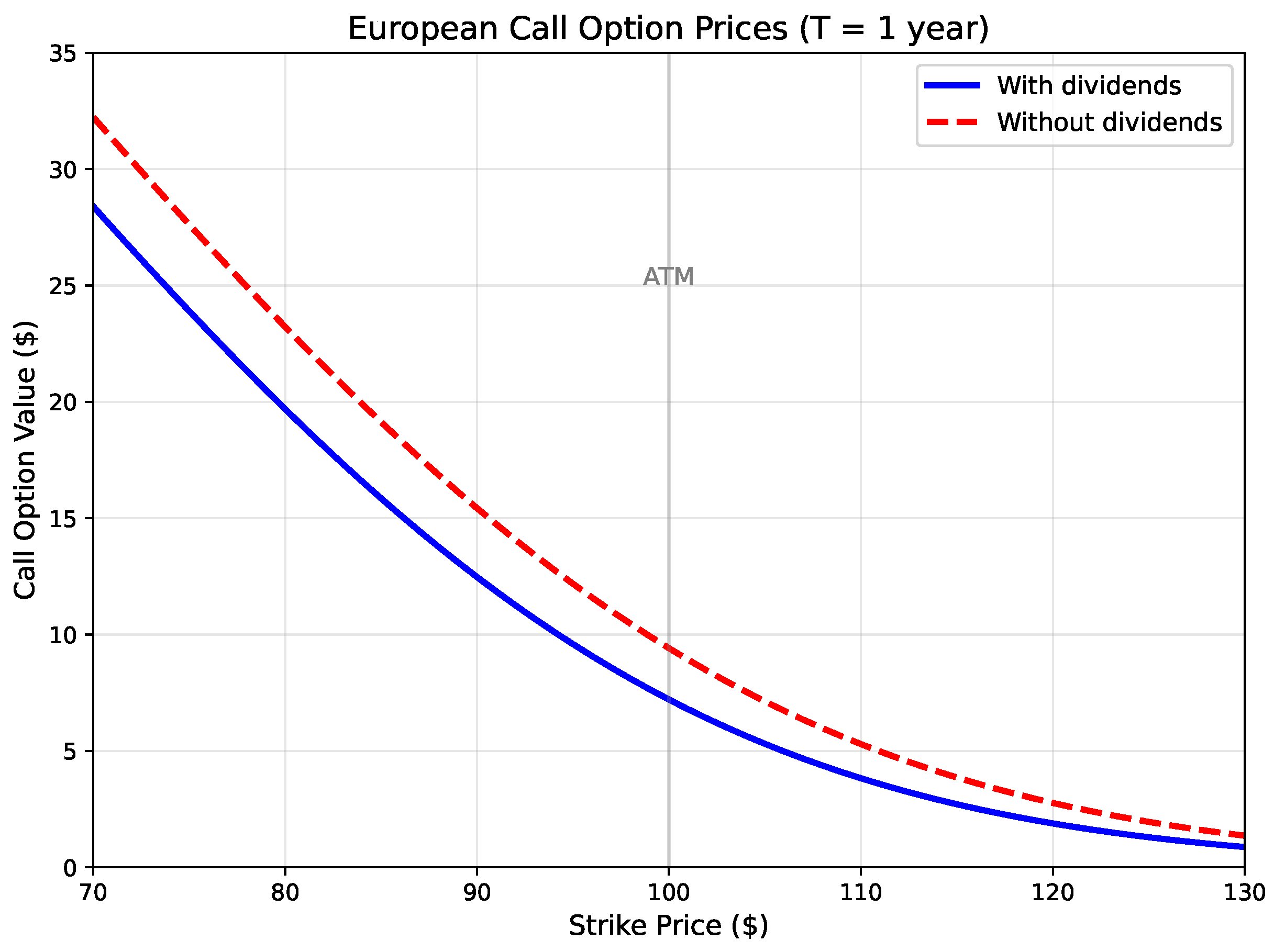
  • At-the-money call value decreases from $9.41 (no dividends) to $7.21 (with dividends), a 23% reduction.
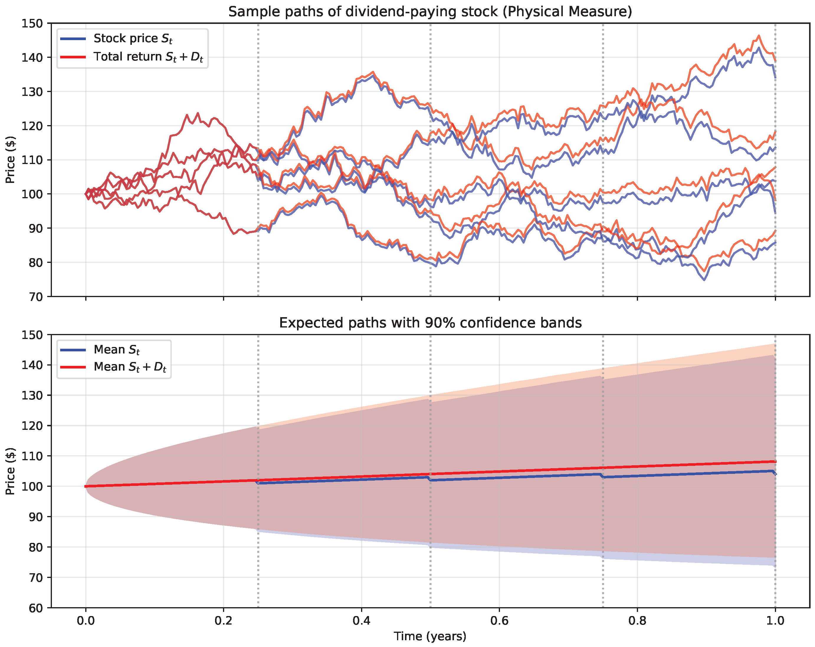
  • Total return including dividends shows approximately 8.2% expected annual return under P .
  • Mean stock price at maturity is $104.03 (excluding dividends), with 90% confidence interval [$73.36, $141.72].

5. Conclusions

This paper has developed a unified framework for mathematical finance under general semimartingale models that accommodate dividend payments, negative asset prices, and unbounded jumps. Our main contributions are the following:
  • Theoretical unification: We provided rigorous conditions under which the semimartingale property is preserved when moving between nominal and discounted frameworks, filling a gap in the literature.
  • Dividend treatment: We extended the classical framework to incorporate general dividend processes, with precise conditions ( [ N , D i ] c = 0 ) ensuring the self-financing property transfers correctly.
  • Admissibility concepts: We clarified various notions of admissible strategies and justified our choice of the economically meaningful bounded-below condition.
  • Practical application: We demonstrated the framework’s relevance through a comprehensive application to dividend-paying equity markets with discrete payments.
  • Transaction cost robustness: We showed that our theoretical results remain valid under small transaction costs, providing a foundation for more realistic market models.
A particularly promising area for future research is the pricing of futures contracts in energy markets. Energy markets present unique challenges that require the full generality of our framework: they exhibit unbounded jumps and frequently experience negative prices, necessitating sigma martingale models rather than traditional martingale approaches. Additionally, futures contracts inherently involve cash flows through margin payments and mark-to-market settlements, making the dividend/cash flow extensions developed in this paper essential. The combination of these features—potential price negativity, unbounded jumps, and intermediate cash flows—makes energy futures an ideal application domain where our general semimartingale framework with dividends becomes not just useful but necessary.
By establishing this general framework and demonstrating its practical relevance through a real market application, we hope to provide a solid mathematical foundation for future developments in mathematical finance that can handle the increasingly complex behaviors observed in modern financial markets.

Funding

This research received no external funding.

Data Availability Statement

No new data were created or analyzed in this study. Data sharing is not applicable to this article.

Conflicts of Interest

The authors declare no conflicts of interest.

Appendix A. Referenced Results

This appendix contains well-known results that were referenced in the paper. Their proofs can be found in [38,52].
Theorem A1.
Let X S d be a d-dimensional topological semimartingale and H L ( X ) . Then, the following hold:
(a) 
For α , β R and J L ( X ) ,
( α H + β J ) L ( X ) and ( α H + β J ) X = α H X + β J X
Hence, L ( X )   i s   a   v e c t o r   s p a c e .
(b) 
I f   Y S d and H L ( X ) L ( Y ) , t h e n   H L ( X L ( X + Y )   a n d
H ( X + Y ) = H X + H X
(c) 
( Δ ( H X ) s ) = H s Δ X s almost surely, for all s 0 .
(d) 
( H X ) T = ( H 1 0 , T ) X = ( H X T )   f o r   a n y   s t o p p i n g   t i m e   T .
(e) 
L e t   X = ( X 1 , , X d ) ,   H = ( H 1 , , H d )   w i t h   H i L ( X i ) ,   a n d   K = ( K 1 , , K d )   b e   p r e d i c t a b l e .   T h e n ,
( K ( H X ) ) = ( K H ) X
w h e n e v e r   t h e   r e l e v a n t   i n t e g r a l s   e x i s t .   C o n c r e t e l y ,   K i L ( H i X i )  if and only if K i H i L ( X i ) .
(f) 
If X is an FV semimartingale, then H X   c o i n c i d e s   w i t h   t h e   u s u a l   p a t h w i s e   R i e m a n n S t i e l t j e s   i n t e g r a l .
(g) 
If Q P , the notion of integrability H L ( X ) does not change, and H X agrees Q -a.s. with the same process defined under P .
Theorem A2.
Let X , Y be two semimartingales. Then, the product process X Y is again a semimartingale, and the following decomposition holds:
X Y = X Y + Y X + [ X , Y ] .
Theorem A3.
A sigma martingale X is a local martingale if and only if X is locally integrable.
Theorem A4.
 Let X , Y S d . Then, [ X , Y ] is, in each component, a finite variation process and a semimartingale, and it satisfies the following properties:
(a) 
[ X , Y ] 0 = X 0 Y 0 and Δ [ X , Y ] i , j = Δ X i Δ Y j .
(b) 
For any stopping time T, we have
[ X T , Y ] = [ X , Y T ] = [ X T , Y T ] = [ X , Y ] T .
(c) 
The quadratic variation [ X , X ] is a positive, increasing process.
(d) 
If X is an FV process, then
[ X , Y ] t = X 0 Y 0 + 0 < s t Δ X s Δ Y s .
Theorem A5.
(a) 
A d-dimensional process X is a topological semimartingale if and only if each of its d components is a topological semimartingale in the one-dimensional sense.
(b) 
A process that is locally a topological semimartingale or prelocally a topological semimartingale is automatically a topological semimartingale (i.e., the property is preserved under localization).
(c) 
If Q P , then any topological semimartingale under P remains a topological semimartingale under Q .
Remark A1.
The space of semimartingales exhibits notable stability properties. For instance, if f : R R is a convex function and X is a semimartingale, then the process f ( X ) is again a semimartingale.
Lemma A1
(Ansel–Stricker Lemma). Let X be a one-dimensional sigma martingale that is bounded from below (for instance X 0 ). Then, X is a local martingale and also a supermartingale. Similarly, if X is bounded from above, then X is a submartingale.
Theorem A6.
 Let B ( t ) be Brownian motion. Then, the following processes are martingales:
(a) 
B ( t ) ;
(b) 
B ( t ) 2 t ;
(c) 
exp u B ( t ) u 2 2 t , for any u R .
Theorem A7.
 Let B ( t ) be Brownian motion. Then,
lim t B ( t ) t = 0 a . s .

References

  1. Bachelier, L. Théorie de la spéculation. In Proceedings of the Annales Scientifiques de l’École Normale Supérieure; Société Mathématique de France: Paris, France, 1900; Volume 17, pp. 21–86. [Google Scholar]
  2. Itô, K. Stochastic integral. Proc. Imp. Acad. 1944, 20, 519–524. [Google Scholar] [CrossRef]
  3. Itô, K. On a stochastic integral equation. Proc. Jpn. Acad. 1946, 22, 32–35. [Google Scholar] [CrossRef]
  4. Itô, K. Stochastic differential equations in a differentiable manifold. Nagoya Math. J. 1950, 1, 35–47. [Google Scholar] [CrossRef]
  5. Itô, K. Multiple Wiener integral. J. Math. Soc. Jpn. 1951, 3, 157–169. [Google Scholar] [CrossRef]
  6. Itô, K. On a formula concerning stochastic differentials. Nagoya Math. J. 1951, 3, 55–65. [Google Scholar] [CrossRef]
  7. Itô, K. On Stochastic Differential Equations; Memoirs of the American Mathematical Society; American Mathematical Society: Providence, RI, USA, 1951; Volume 4. [Google Scholar]
  8. Black, F.; Scholes, M. The Pricing of Options and Corporate Liabilities. J. Political Econ. 1973, 81, 637–654. [Google Scholar] [CrossRef]
  9. Doob, J. Stochastic Processes; Wiley Classics Library; John Wiley & Sons: New York, NY, USA, 1953; Volume 7. [Google Scholar]
  10. Meyer, P.A. A decomposition theorem for supermartingales. Ill. J. Math. 1962, 6, 193–205. [Google Scholar] [CrossRef]
  11. Meyer, P.A. Decomposition of supermartingales: The uniqueness theorem. Ill. J. Math. 1963, 7, 1–17. [Google Scholar] [CrossRef]
  12. Kunita, H.; Watanabe, S. On square integrable martingales. Nagoya Math. J. 1967, 30, 209–245. [Google Scholar] [CrossRef]
  13. Meyer, P.A. Intégrales stochastiques I. Semin. Probab. Strasbg. 1967, 39, 72–94. [Google Scholar]
  14. Meyer, P.A. Intégrales stochastiques II. Semin. Probab. Strasbg. 1967, 1, 95–117. [Google Scholar]
  15. Meyer, P.A. Intégrales stochastiques III. Semin. Probab. Strasbg. 1967, 1, 118–141. [Google Scholar]
  16. Meyer, P.A. Intégrales stochastiques IV. Semin. Probab. Strasbg. 1967, 1, 142–162. [Google Scholar]
  17. Doléans-Dade, C.; Meyer, P.A. Intégrales stochastiques par rapport aux martingales locales. In Séminaire de Probabilités IV, Université de Strasbourg; Lecture Notes in Mathematics; Springer: Berlin/Heidelberg, Germany, 1970; Volume 124, pp. 77–107. [Google Scholar]
  18. Meyer, P. Un Cours sur les Intégrales Stochastiques. In Séminaire de Probabilités 1967–1980; Lecture Notes in Mathematics; Émery, M., Yor, M., Eds.; Springer: Berlin/Heidelberg, Germany, 2002; Volume 1771, pp. 174–329. [Google Scholar] [CrossRef]
  19. Jacod, J. Calcul Stochastique et Problèmes de Martingales; Lecture Notes in Mathematics; Springer: Berlin/Heidelberg, Germany, 1979; Volume 714, p. x+280. [Google Scholar]
  20. Chou, C.S.; Meyer, P.A.; Stricker, C. Sur les intégrales stochastiques de processus prévisibles non bornés. In Séminaire de Probabilités XIV, 1978/79; Lecture Notes in Mathematics; Springer: Berlin/Heidelberg, Germany, 1980; Volume 784, pp. 128–139. [Google Scholar] [CrossRef]
  21. Jacod, J. Intégrales stochastiques par rapport à une semimartingale vectorielle et changements de filtration. In Séminaire de Probabilités XIV, 1978/79; Lecture Notes in Mathematics; Springer: Berlin/Heidelberg, Germany, 1980; Volume 784, pp. 161–172. [Google Scholar]
  22. Harrison, J.M.; Pliska, S.R. Martingales and stochastic integrals in the theory of continuous trading. Stoch. Process. Their Appl. 1981, 11, 215–260. [Google Scholar] [CrossRef]
  23. Delbaen, F.; Schachermayer, W. A general version of the fundamental theorem of asset pricing. Math. Ann. 1994, 300, 463–520. [Google Scholar] [CrossRef]
  24. Delbaen, F.; Schachermayer, W. The Fundamental Theorem of Asset Pricing for Unbounded Stochastic Processes. Math. Ann. 1998, 312, 215–250. [Google Scholar] [CrossRef]
  25. Jarrow, R. The arbitrage theory of capital asset pricing and the martingale property of asset prices. Econ. Theory 1999, 13, 253–264. [Google Scholar]
  26. Bichteler, K. Stochastic Integration and Lp-Theory of Semimartingales. Ann. Probab. 1981, 9, 49–89. [Google Scholar] [CrossRef]
  27. Kabanov, Y.; Safarian, M. Markets with Transaction Costs: Mathematical Theory; Springer: Berlin/Heidelberg, Germany, 2016. [Google Scholar]
  28. Fontana, C. Weak and strong no-arbitrage conditions for continuous financial markets. Int. J. Theor. Appl. Financ. 2015, 18, 1550005. [Google Scholar] [CrossRef]
  29. Platen, E.; Heath, D. A Benchmark Approach to Quantitative Finance; Springer: Berlin/Heidelberg, Germany, 2006. [Google Scholar]
  30. Korn, R. Optimal portfolios with a positive lower bound on final wealth. Quant. Financ. 2005, 5, 315–321. [Google Scholar] [CrossRef]
  31. Rogers, L.C.G.; Williams, D. Diffusions, Markov Processes and Martingales: Volume 2, Itô Calculus; Cambridge Mathematical Library, Cambridge University Press: Cambridge, UK, 2000; p. xvi+480. [Google Scholar]
  32. Jarrow, R. Continuous-Time Asset Pricing Theory: A Martingale-Based Approach, 2nd ed.; Springer Finance, Springer International Publishing: Cham, Switzerland, 2021. [Google Scholar]
  33. Whaley, R.E. Valuation of American call options on dividend-paying stocks: Empirical tests. J. Financ. Econ. 1982, 10, 29–58. [Google Scholar] [CrossRef]
  34. Harvey, C.R.; Whaley, R.E. Dividends and S&P 100 index option valuation. J. Futur. Mark. 1992, 12, 123–137. [Google Scholar] [CrossRef]
  35. Wilkens, S.; Wimschulte, J. The pricing of dividend futures in the European market: A first empirical analysis. J. Deriv. Hedge Funds 2009, 16, 136–143. [Google Scholar] [CrossRef]
  36. Sohns, M. The General Semimartingale Model with Dividends. In Proceedings of the Results of Social Science Research with Economic and Financial Effects (10th Annual Conference), Prague, Czech Republic, 15 November 2023. [Google Scholar] [CrossRef]
  37. Cohen, S.; Elliott, R. Stochastic Calculus and Applications; Probability and Its Applications; Springer: New York, NY, USA, 2015. [Google Scholar] [CrossRef]
  38. Sohns, M. General Stochastic Vector Integration—Three Approaches. Preprints 2025. [Google Scholar] [CrossRef]
  39. Guasoni, P. No arbitrage under transaction costs, with fractional Brownian motion and beyond. Math. Financ. 2006, 16, 569–582. [Google Scholar] [CrossRef]
  40. Kabanov, Y.M.; Stricker, C. Hedging and liquidation under transaction costs in currency markets. Financ. Stochastics 2001, 5, 237–248. [Google Scholar] [CrossRef]
  41. Mixon, S. Option markets and implied volatility: Past versus present. J. Financ. Econ. 2009, 94, 171–191. [Google Scholar] [CrossRef]
  42. Ansel, J.P.; Stricker, C. Lois de martingale, densités et décomposition de Föllmer Schweizer. Ann. Henri Poincaré Inst. (B) Probab. Stat. 1992, 28, 375–392. [Google Scholar]
  43. Kardaras, C.; Platen, E. On the semimartingale property of discounted asset-price processes. Stoch. Process. Their Appl. 2011, 121, 2678–2691. [Google Scholar] [CrossRef]
  44. Bingham, N.; Kiesel, R. Risk-Neutral Valuation: Pricing and Hedging of Financial Derivatives, 2nd ed.; Springer Finance, Springer: London, UK, 2013. [Google Scholar] [CrossRef]
  45. Elliott, R.; Kopp, P. Mathematics of Financial Markets, 2nd ed.; Springer Finance, Springer: New York, NY, USA, 2005; p. xii+352. [Google Scholar]
  46. Pascucci, A. PDE and Martingale Methods in Option Pricing; Bocconi & Springer Series; Springer: Berlin/Heidelberg, Germany, 2011. [Google Scholar] [CrossRef]
  47. Geman, H.; Karoui, N.; Rochet, J. Changes of Numéraire, Changes of Probability Measure and Option Pricing. J. Appl. Probab. 1995, 32, 443–458. [Google Scholar] [CrossRef]
  48. Ebenfeld, S. Grundlagen der Finanzmathematik: Mathematische Methoden, Modellierung von Finanzmärkten und Finanzprodukten; Schäffer-Poeschel: Stuttgart, Germany, 2007. [Google Scholar]
  49. Klein, I.; Schmidt, T.; Teichmann, J. No Arbitrage Theory for Bond Markets. In Advanced Modelling in Mathematical Finance; Springer: Berlin/Heidelberg, Germany, 2016; pp. 381–421. [Google Scholar] [CrossRef]
  50. Qin, L.; Linetsky, V. Long-Term Risk: A Martingale Approach. Econometrica 2017, 85, 299–312. [Google Scholar] [CrossRef]
  51. Herdegen, M.; Schweizer, M. Strong bubbles and strict local martingales. Int. J. Theor. Appl. Financ. 2016, 19, 1650022. [Google Scholar] [CrossRef]
  52. Sohns, M. σ-Martingales: Foundations, Properties, and a New Proof of the Ansel–Stricker Lemma. Mathematics 2025, 13, 682. [Google Scholar] [CrossRef]
  53. Shiryaev, A.N. Essentials of Stochastic Finance; Advanced Series on Statistical Science & Applied Probability; World Scientific Publishing Co., Inc.: River Edge, NJ, USA, 1999; Volume 3, p. xvi+834. [Google Scholar] [CrossRef]
  54. Shiryaev, A.N.; Cherny, A. Vector stochastic integrals and the fundamental theorems of asset pricing. Proc. Steklov Inst. Math. Interperiodica Transl. 2002, 237, 6–49. [Google Scholar]
  55. Filipovic, D. Term-Structure Models. A Graduate Course; Springer: Berlin/Heidelberg, Germany, 2009. [Google Scholar] [CrossRef]
  56. Biagini, F. Second Fundamental Theorem of Asset Pricing. Encycl. Quant. Financ. 2010, 4, 1623–1628. [Google Scholar] [CrossRef]
  57. Musiela, M.; Rutkowski, M. Martingale Methods in Financial Modelling, 2nd ed.; Stochastic Modelling and Applied Probability; Springer: Berlin/Heidelberg, Germany, 2005; Volume 36, p. xx+638. [Google Scholar]
  58. Klebaner, F.C. Introduction to Stochastic Calculus with Applications, 2nd ed.; Imperial College Press: London, UK, 2005; p. xvi+412. [Google Scholar]
  59. Øksendal, B. Stochastic Differential Equations: An Introduction with Applications, 6th ed.; Universitext; Springer: Berlin/Heidelberg, Germany, 2010; p. 404. [Google Scholar] [CrossRef]
  60. Kuo, H.H. Introduction to Stochastic Integration, 1st ed.; Universitext; Springer: New York, NY, USA, 2006; p. x+278. [Google Scholar] [CrossRef]
  61. Yan, J.A. Introduction to Stochastic Finance, 1st ed.; Universitext; Springer: Singapore, 2018. [Google Scholar] [CrossRef]
  62. Harrison, J.M.; Pliska, S.R. A stochastic calculus model of continuous trading: Complete markets. Stoch. Process. Their Appl. 1983, 15, 313–316. [Google Scholar] [CrossRef]
  63. Cox, A.; Hobson, D. Local martingales, bubbles and option prices. Financ. Stoch. 2005, 9, 477–492. [Google Scholar] [CrossRef]
  64. Jarrow, R.A.; Protter, P.; Shimbo, K. Asset Price Bubbles in Complete Markets. In Advances in Mathematical Finance; Fu, M.C., Jarrow, R.A., Yen, J.Y.J., Elliott, R.J., Eds.; Applied and Numerical Harmonic Analysis; Birkhäuser Boston: Boston, MA, USA, 2007; pp. 97–121. [Google Scholar] [CrossRef]
  65. Jarrow, R.; Protter, P.; Shimbo, K. Asset Price Bubbles in Incomplete Markets. Math. Financ. 2010, 20, 145–185. [Google Scholar] [CrossRef]
  66. Merton, R. Option Pricing when Underlying Stock Returns are Discontinuous. J. Financ. Econ. 1976, 3, 125–144. [Google Scholar] [CrossRef]
  67. Wilmott, P. Derivatives: The Theory and Practice of Financial Engineering; John Wiley & Sons: Chichester, UK, 1998. [Google Scholar]
Figure 1. Logical dependencies in the general semimartingale model. Solid arrows indicate direct dependencies; dashed arrows indicate alternative paths.
Appliedmath 05 00097 g001
Figure 2. Relationship between nominal and discounted frameworks.
Appliedmath 05 00097 g002
Figure 3. Sample paths of dividend-paying stock under the physical measure P . The blue line shows the stock price S t with quarterly drops, the red line shows the continuous total return process S t + D t , and vertical dotted lines mark dividend payment dates.
Appliedmath 05 00097 g003
Figure 4. Call option prices versus strike, comparing prices with dividends (solid) and without dividends (dashed). The dividend adjustment significantly reduces option values, particularly for in-the-money calls.
Appliedmath 05 00097 g004
Disclaimer/Publisher’s Note: The statements, opinions and data contained in all publications are solely those of the individual author(s) and contributor(s) and not of MDPI and/or the editor(s). MDPI and/or the editor(s) disclaim responsibility for any injury to people or property resulting from any ideas, methods, instructions or products referred to in the content.

