Mathematical Model for Economic Growth, Corruption and Unemployment: Analysis of the Effects of a Time Delay in the Economic Growth

Abstract

In this article, we propose a nonlinear mathematical model that incorporates a discrete time delay. The model is used to analyze the dynamics of a socioeconomic system that includes economic growth, corruption, and unemployment. We introduce the time delay in the logistic economic growth term due to the effect of the previous state of the economic growth on its current state. A local stability analysis is performed to investigate the dynamics of the socioeconomic system. We established conditions for the existence of Hopf bifurcations and the appearance of economic limit cycles. We found threshold values for the discrete-time delay in which these Hopf bifurcations occur. We corroborate the theoretical findings by performing numerical simulations for a variety of scenarios. We find various interesting socioeconomic situations where different socioeconomic limit cycles occur. Finally, we present a discussion and future directions of research.

1. Introduction

Researchers have developed mathematical models to study socioeconomic systems and gain further insight into their dynamics [1,2,3,4]. Among the most famous mathematical models for economic growth, we have the Solow model and many variants of it [5,6,7]. Many mathematical models that have been studied for socioeconomic systems are based on differential equations [8,9,10]. In [11], a three-dimensional mathematical model based on a nonlinear system of differential equations was used to study unemployment. In [12], a mathematical model to study poverty and crime was proposed. Among mathematical models based on differential equations, there are models that use delay differential equations to represent a delayed effect of some factors on others [13,14,15,16]. For example, the Solow model with spatial dependence and time delay has been analyzed [17]. In [18], a mathematical model with delays was used to study unemployment, and Hopf bifurcation was analyzed. In [19], a financial system that includes interest rate, investment demand, price index, average profit margin, and time delay was investigated. The existence of a Hopf bifurcation in a one-sector growth model with delay has been demonstrated [20].

Bifurcations are relevant in the study of dynamical systems, since a small change in the value of a parameter can cause an abrupt change in the qualitative behavior of the system [21,22,23]. Thus, the study of bifurcation points and bifurcation boundaries in mathematical models for economics can be crucial to understanding the potential outcomes of the economy of a nation [24,25,26,27]. One relevant and important bifurcation in economic models is the Hopf bifurcation, since it gives conditions such that economic cycles arise [28,29,30,31,32]. Previous works have found Hopf bifurcations in mathematical models that studied socioeconomic factors such as inflation, corruption, and unemployment [33,34,35,36]. The occurrence of Hopf bifurcations can be due to the parameters of the model and also due to time delays in the model [19,37,38,39]. However, in many other economic models, a Hopf bifurcation arises from a change in the value of a parameter different from a time delay [23,36,40,41].

In this paper, the mathematical model includes three main socioeconomic factors. The first is economic growth, which refers to the increase in the economy of a nation over time and is commonly measured by the gross domestic product (GDP) [42,43]. The second factor is corruption, which includes a wide variety of aspects such as tax evasion. The importance of including corruption in the model is that it negatively affects the economy of a nation and its citizens [44]. The third socioeconomic factor that the mathematical model considers is unemployment. This is also a crucial aspect of the economy, as it affects inflation [45,46,47,48,49]. Moreover, unemployment and economic growth are correlated [50,51,52]. Thus, in this work, we study the dynamics of economic growth, corruption, and unemployment considering feedback in the economic growth by means of a discrete time delay. Previous works have considered similar feedback in economic models [53,54,55,56,57].

In this article, we extend a socioeconomic mathematical model for economic growth, corruption, and unemployment by incorporating a discrete time delay into the model to account for a more realistic real-world scenario. Through local stability and bifurcation analysis for systems with incorporated discrete time delays, this research aims to provide deeper insight into the complex dynamics among these key economic factors. By exploring how delays and nonlinearities affect system behavior, this study helps to determine situations that may drive cyclical fluctuations, instability, or unexpected transitions in economic indicators. These situations, often not included in simpler models, are essential in capturing the complicated realities of economic systems.

This article is structured as follows. In Section 2, we present the mathematical model. In Section 3, the stability analysis of the model is presented. Section 4 shows the numerical results that support the theoretical findings. Finally, Section 5 is devoted to present the conclusions.

2. Mathematical Model

In this section, we present a mathematical model for economic growth, corruption, and unemployment with a logistic growth term for economic growth. The model is based on a nonlinear system of ordinary differential equations and is given by

$$\begin{array}{cc}\hfill {\displaystyle \frac{dG\left(t\right)}{dt}}& =r_{1}G\left(t\right)\left(1-{\displaystyle \frac{G\left(t\right)}{K_1}}\right)-{\displaystyle \frac{\beta G\left(t\right)C\left(t\right)}{1+a\beta G\left(t\right)}},\hfill \\ \hfill {\displaystyle \frac{dC\left(t\right)}{dt}}& =\varphi {\displaystyle \frac{\beta G\left(t\right)C\left(t\right)}{1+a\beta G\left(t\right)}}-\mu C\left(t\right),\hfill \\ \hfill {\displaystyle \frac{dU\left(t\right)}{dt}}& =r_{2}U\left(t\right)\left(1-{\displaystyle \frac{U\left(t\right)+\xi G\left(t\right)}{K_2}}\right)-\kappa U\left(t\right),\hfill \end{array}$$

(1)

where $G\left(t\right)$ is economic growth, $C\left(t\right)$ is the corruption density, and $U\left(t\right)$ is unemployment density [58]. With regard to the parameters, $r_1$ is the intrinsic growth rate of the economy, $r_2$ is the unemployment growth rate, $K_1$ is the economic carrying capacity, $K_2$ is the maximum level of unemployment, $\beta$ is the rate at which corrupted officials encounter economic resources, a is the average time spent processing corruption (handling time), $\varphi$ is the specific conversion rate at which corrupt officials convert accessed resources into personal gains, $\mu$ represents factors that reduce corruption like detection and enforcement, $\xi$ is the constant rate at which economic growth creates new job opportunities, and $\kappa$ is the new private business density rate. All parameters $r_1,r_2,K_1,K_2,\beta ,a,\varphi ,\mu ,\xi ,$ and $\kappa$ are positive. Furthermore, in [58], it is assumed that $\kappa <r_2$ or $r_2-\kappa >0$ ($\kappa -r_2<0$). The next section is devoted to the stability analysis and finding the conditions for the existence of Hopf bifurcations for the mathematical model (1).

Proposed Mathematical Model with Delay

Economic growth is the increase in the production of goods and services in the economy over a certain period of time and is measured primarily by the country’s gross domestic product (GDP). The importance of economic growth in any nation cannot be overemphasized. A healthy economic growth alleviates poverty, improves standard of living, promotes technological advancement, provides basic amenities and infrastructure, fosters job creation, enhances overall quality of life, etc.

We will take into account what happens when there is a delay in economic growth and explore how this delay affects the entire system. There are several factors that hinder economic growth in any country. Some of these factors are lack of investment in basic infrastructure and technology, natural disasters, poor governance and government policies, low productivity, political instability, general insecurity, increased population aging, and many more. Here, we will consider a system where there is a delay in economic growth by introducing a “time lag” or a “delay parameter $\tau$” in Equation (1), meaning that the economic system takes time to react to stimuli, causing a lag in the growth process. With this, we will explore the Hutchinson-type delay in the $G/K1$ term, where the economic growth rate depends on previous growth at a previous time. Realistically, this time delay reflects the delayed realization of the effects of past economic growth on the system’s carrying capacity, the time it takes for resource constraints to affect the system, institutional or policy reaction lags, delayed perception or response to economic indicators, and so on. Thus, we have

$$\begin{array}{cc}\hfill {\displaystyle \frac{dG\left(t\right)}{dt}}& =r_{1}G\left(t\right)\left(1-{\displaystyle \frac{G(t-\tau )}{K_1}}\right)-{\displaystyle \frac{\beta G\left(t\right)C\left(t\right)}{1+a\beta G\left(t\right)}},\hfill \\ \hfill {\displaystyle \frac{dC\left(t\right)}{dt}}& =\varphi {\displaystyle \frac{\beta G\left(t\right)C\left(t\right)}{1+a\beta G\left(t\right)}}-\mu C\left(t\right),\hfill \\ \hfill {\displaystyle \frac{dU\left(t\right)}{dt}}& =r_{2}U\left(t\right)\left(1-{\displaystyle \frac{U\left(t\right)+\xi G\left(t\right)}{K_2}}\right)-\kappa U\left(t\right),\hfill \end{array}$$

(2)

Since the delay is incorporated in $G\left(t\right)$, we introduce a constant initial history function that accounts for all G values not only at time $t=0$ but for all times $t\in [-\tau ,0]$. For the state variables $C\left(t\right)$ and $U\left(t\right)$, no history function is needed since they do not include the time delay [59,60,61]. In addition, all the state variables are considered non-negative. Therefore,

$G\left(\nu \right)=G_0\ge 0$ and $\nu \in [-\tau ,0]$, $C\left(0\right)=C_0\ge 0$ and $U\left(0\right)=U_0\ge 0.$

3. Stability Analysis of Equilibria

With the inclusion of the delay parameter $\tau$, we will investigate the stability of the fixed points of the model (2). First, we find the equilibrium points, compute the Jacobian matrix of the model at these points, and analyze conditions for stability and the possibility of periodic solutions that may arise due to $\tau$.

3.1. Equilibrium Points

To obtain the equilibrium points, the right-hand side of system (2) is set to zero, and then the equations are solved to determine the fixed points of the system. Dropping the time dependence, one gets

$$\begin{array}{cc}\hfill r_{1}G\left(1-{\displaystyle \frac{G}{K_1}}\right)-{\displaystyle \frac{\beta GC}{1+a\beta G}}& =0,\hfill \\ \hfill \varphi {\displaystyle \frac{\beta GC}{1+a\beta G}}-\mu C& =0,\hfill \\ \hfill r_{2}U\left(1-{\displaystyle \frac{U+\xi G}{K_2}}\right)-\kappa U& =0.\hfill \end{array}$$

(3)

The equilibrium points of system (2) are described by their qualitative nature or interpretation of the state represented by each of them.

• The trivial equilibrium point $E_0=(0,0,0)$.
• The axial equilibrium point $E_1=(0,0,{\displaystyle \frac{K_2(r_2-\kappa )}{r_2}})$.
• The axial equilibrium point $E_2=(K_1,0,0)$.
• Economic-specific equilibrium point $E_3=\left(K_1,0,K_2\left(1-{\displaystyle \frac{\kappa }{r_2}}\right)-\xi K_1\right)$.
• Unemployment-free equilibrium $E_4=\left({\displaystyle \frac{\mu }{\beta (\varphi -a\mu )}},{\displaystyle \frac{\varphi r_1}{1+a\beta K_1}}\left({\displaystyle \frac{\beta K_1}{1+a\beta K_1}}-\mu \right),0\right)$.
• Positive interior equilibrium $E_5=\left({\displaystyle \frac{\mu }{\beta (\varphi -a\mu )}},{\displaystyle \frac{\varphi r_1}{1+a\beta K_1}}\left({\displaystyle \frac{\beta K_1}{1+a\beta K_1}}-\mu \right),{\displaystyle \frac{K_2\left(r_2-\kappa \right)\left(a\mu -\varphi \right)\beta +\mu r_2\xi }{\beta \left(a\mu -\varphi \right)r_2}}\right)$.

3.2. Computing the Jacobian Matrix of the System

Let $X=(G,C,U)$ be the state vector. The Jacobian matrix of system (2) is $J=J_0+e^{-\lambda \tau }{J}_{\tau }$, where $J_0$ is the Jacobian matrix of system (2) without the delay and $J_{\tau }$ is the Jacobian matrix of system (2) with respect to the delay $\tau$ (for interested readers, see [59,60,61]). Thus, one has

$$\begin{array}{c}\hfill J=\left(\begin{array}{ccc}{r}_1\left(1-{\displaystyle \frac{G^{*}(1+e^{-\lambda \tau })}{K_1}}\right)-{\displaystyle \frac{\beta C^{*}}{{(a\beta G^{*}+1)}^2}}& -{\displaystyle \frac{\beta G^{*}}{a\beta G^{*}+1}}& 0\\ \\ {\displaystyle \frac{\varphi \beta C^{*}}{{(a\beta G^{*}+1)}^2}}& {\displaystyle \frac{\varphi \beta G^{*}}{a\beta G^{*}+1}}-\mu & 0\\ \\ -{\displaystyle \frac{{\mathit{r}}_{\mathit{2}}\xi U^{*}}{{\mathit{K}}_{\mathit{2}}}}& 0& {\mathit{r}}_{\mathit{2}}\left(1-{\displaystyle \frac{G^{*}\xi +2U^{*}}{{\mathit{K}}_{\mathit{2}}}}\right)-\kappa \end{array}\right).\end{array}$$

(4)

Next, we analyze this Jacobian matrix at all the equilibrium points $(G^{*},C^{*},U^{*})$ and explore their stability. We also examine the possibility for the existence of Hopf bifurcation (economic limit cycles) at each equilibrium point. If all eigenvalues of the Jacobian evaluated at that equilibrium point are strictly real, Hopf bifurcation is ruled out. Otherwise, we check for a pair of simple conjugate purely imaginary roots crossing the imaginary axis. To do this, we set $\lambda =iv,v>0,v\in \mathbb{R}$, substitute into the characteristic equation, separate into real and imaginary parts, and solve for v and the corresponding critical delay $\tau$. Lastly, we verify the transversality condition [59,60,61].

3.3. Stability Analysis and Possible Hopf Bifurcation Arising from $E_0=(0,0,0)$

Here, we will analyze the eigenvalues of the Jacobian matrix (4) evaluated at $E_0$. The Jacobian matrix evaluated at $E_0$ is

$$\begin{array}{c}\hfill J\left(E_0\right)=\left[\begin{array}{ccc}{r}_1& 0& 0\\ \\ 0& -\mu & 0\\ \\ 0& 0& r_2-\kappa \end{array}\right].\end{array}$$

(5)

We can see that this is a diagonal matrix and its eigenvalues are the diagonal entries. Thus, the eigenvalues are ${\lambda }_1=r_1,{\lambda }_2=-\mu$ and ${\lambda }_3=r_2-\kappa$. The first eigenvalue ${\lambda }_1=r_1>0$; therefore, $E_0$ is always unstable. In dynamical systems, a Hopf bifurcation occurs when a pair of complex conjugate eigenvalues from the linearized flow at an equilibrium point transition to purely imaginary values. We see here that all the eigenvalues of $E_0$ are strictly real, so a Hopf bifurcation cannot arise from this point [21,23].

3.4. Stability Analysis and Existence of Hopf Bifurcation Arising from $E_1=(0,0,{\displaystyle \frac{K_2(r_2-\kappa )}{r_2}})$

Here, we will analyze the eigenvalues arising from evaluating the Jacobian matrix (4) at $E_1$. The Jacobian matrix evaluated at $E_1$ is

$$\begin{array}{c}\hfill J\left(E_1\right)=\left[\begin{array}{ccc}{r}_1& 0& 0\\ \\ 0& -\mu & 0\\ \\ (\kappa -r_2)\xi & 0& \kappa -r_2\end{array}\right].\end{array}$$

(6)

The eigenvalues of the Jacobian matrix in Equation (6) are ${\lambda }_1=r_1,{\lambda }_2=-\mu$ and ${\lambda }_3=\kappa -r_2$. Again, the eigenvalue ${\lambda }_1=r_1>0$; therefore, $E_1$ is unstable. Clearly, all the eigenvalues of $E_1$ are strictly real, so a Hopf bifurcation cannot arise from this steady state [21,23].

3.5. Stability Analysis and Existence of Hopf Bifurcation Arising from $E_2=(K_1,0,0)$

The Jacobian matrix (4) evaluated at $E_2$ is

$$\begin{array}{c}\hfill J\left(E_2\right)=\left[\begin{array}{ccc}-r_1{e}^{-\lambda \tau }& -{\displaystyle \frac{\beta K_1}{a\beta K_1+1}}& 0\\ \\ 0& {\displaystyle \frac{\varphi \beta K_1}{a\beta K_1+1}}-\mu & 0\\ \\ 0& 0& {\displaystyle \frac{K_2\left(r_2-\kappa \right)-r_2{K}_1\xi }{K_2}}\end{array}\right].\end{array}$$

(7)

Note the presence of the exponential term in (7). We will compute the characteristic equation and analyze it for the local stability of $E_2$.

$$\begin{array}{c}\hfill |J\left(E_2\right)-\lambda I|=\left|\begin{array}{ccc}-r_1{e}^{-\lambda \tau }-\lambda & -{\displaystyle \frac{\beta K_1}{a\beta K_1+1}}& 0\\ \\ 0& {\displaystyle \frac{\varphi \beta K_1}{a\beta K_1+1}}-\mu -\lambda & 0\\ \\ 0& 0& {\displaystyle \frac{K_2\left(r_2-\kappa \right)-r_2{K}_1\xi }{K_2}}-\lambda \end{array}\right|=0.\end{array}$$

(8)

This determinant is equal to the product of the diagonal entries as follows:

$$\begin{array}{c}\hfill \left(-r_1{e}^{-\lambda \tau }-\lambda \right)\left({\displaystyle \frac{\varphi \beta K_1}{a\beta K_1+1}}-\mu -\lambda \right)\left({\displaystyle \frac{K_2\left(r_2-\kappa \right)-r_2{K}_1\xi }{K_2}}-\lambda \right)=0.\end{array}$$

(9)

When $\tau =0$ (no delay), the characteristic Equation (9) has three real roots (eigenvalues), which are

${\lambda }_1=-r_1<0$,

${\lambda }_2={\displaystyle \frac{\varphi \beta K_1}{a\beta K_1+1}}-\mu <0$ if $\mu >{\displaystyle \frac{\varphi \beta K_1}{a\beta K_1+1}}$ and

${\lambda }_3={\displaystyle \frac{K_2\left(r_2-\kappa \right)-r_2{K}_1\xi }{K_2}}<0$ if $r_2>{\displaystyle \frac{K_2(r_2-\kappa )}{K_1\xi }}$.

With these conditions, the equilibrium point $E_2$ is locally asymptotically stable. This is identical to the results in [58].

Let $\tau >0$ be fixed. Using this as the bifurcation parameter, we can determine the values of $\tau$ such that the steady state of the system changes from local stability to instability. This will shed light on how the delay parameter affects the system. We show that the characteristic Equation (9) has a pair of purely imaginary roots $\lambda =\pm i{v}_0$ that cross from the ${\mathbb{C}}^{-}$ plane to the ${\mathbb{C}}^{+}$ plane.

Theorem 1.

For $\tau ={\tau }_k$, the characteristic Equation (9) has a pair of simple conjugate purely imaginary roots $\lambda =\pm i{v}_0$, where

$$\begin{array}{c}\hfill {\tau }_k={\displaystyle \frac{1}{v_0}}\left({\displaystyle \frac{\pi }{2}}+2\pi k\right),v_0=r_1,\mathrm{with}k=0,1,2,3···\end{array}$$

(10)

and the transversality condition

$$\begin{array}{c}\hfill {\left.{\displaystyle \frac{d(\Re \lambda (\tau \left)\right)}{d\tau }}\right|}_{\tau ={\tau }_k}>0\end{array}$$

(11)

is satisfied.

Proof. 

Using only the transcendental part of (9),

$$\begin{array}{c}\hfill P(\lambda ,\tau )=-\lambda -r_1{e}^{-\lambda \tau }=0,\end{array}$$

(12)

let $\lambda =iv,v>0$ be one root of (12), substituting gives

$$\begin{array}{c}\hfill -iv-r_1{e}^{-iv\tau }=iv+r_1{e}^{-iv\tau }=0,\end{array}$$

(13)

substituting $e^{-iv\tau }=cos\left(v\tau \right)-isin\left(v\tau \right)$ in (13) gives

$$\begin{array}{c}\hfill iv+r_{1}cos\left(v\tau \right)-i{r}_{1}sin\left(v\tau \right)=0,\end{array}$$

then separating the real and imaginary components gives

$$\begin{array}{c}\hfill r_{1}cos\left(v\tau \right)=0,\end{array}$$

(14)

$$\begin{array}{c}\hfill r_{1}sin\left(v\tau \right)=v,\end{array}$$

(15)

Equations (14) and (15) are both satisfied only when $v\tau ={\displaystyle \frac{\pi }{2}}+2\pi k,k=0,1,2,3,···$, and $v=v_0=r_1$.

Next, we verify that $\lambda =\pm iv$ are simple roots. Clearly, ${\left.P(\lambda ,\tau )\right|}_{\lambda =\pm i{v}_0}=0$. Now, ${\displaystyle \frac{dP(\lambda ,\tau )}{d\lambda }}=-1+r_1\tau e^{-\lambda \tau }$. For the derivative,

$$\begin{array}{c}\hfill {\left.{\displaystyle \frac{dP(\lambda ,\tau )}{d\lambda }}\right|}_{\lambda =\pm i{v}_0}=-1+r_1\tau e^{-(\pm i{v}_0)\tau }=-1+r_1\tau cos\left(v_0\tau \right)\pm i{r}_1\tau sin\left(v_0\tau \right).\end{array}$$

(16)

Thus, using Equations (14) and (15) reduces Equation (16) to

$$\begin{array}{c}\hfill {\left.{\displaystyle \frac{dP(\lambda ,\tau )}{d\lambda }}\right|}_{\lambda =\pm i{v}_0}=-1\pm i{v}_0\tau \ne 0.\end{array}$$

(17)

Thus, $\lambda =\pm i{v}_0$ is a pair of simple conjugate purely imaginary roots of (12). Thus, Equation (10) is satisfied.

Finally, we will prove the transversality condition. Suppose $\lambda =u\left(\tau \right)+iv\left(\tau \right)$ is a root of the transcendental Equation (12) where $u\left({\tau }_k\right)=0$, and $v\left({\tau }_k\right)=v_0$. Taking the derivative of the transcendental Equation (12) with respect to the bifurcation parameter $\tau$ gives:

$$\begin{array}{c}\hfill -{\displaystyle \frac{d\lambda }{d\tau }}-r_1{e}^{-\lambda \tau }\left(-\tau {\displaystyle \frac{d\lambda }{d\tau }}-\lambda \right)=0.\end{array}$$

(18)

Also, from (12), $\lambda =-r_1{e}^{-\lambda \tau }$, substituting this in (18) results in

$$\begin{array}{cc}\hfill -{\displaystyle \frac{d\lambda }{d\tau }}+\lambda \left(-\tau {\displaystyle \frac{d\lambda }{d\tau }}-\lambda \right)& =0\hfill \\ \hfill -{\displaystyle \frac{d\lambda }{d\tau }}(1+\lambda \tau )& ={\lambda }^2\hfill \\ \hfill {\displaystyle \frac{d\lambda }{d\tau }}& =-{\displaystyle \frac{{\lambda }^2}{1+\lambda \tau }}.\hfill \end{array}$$

With this complete, we check the sign of the derivative of the real part of $\lambda$,

$$\begin{array}{cc}\hfill {\displaystyle \frac{d\Re \left(\lambda \right(\tau \left)\right)}{d\tau }}={\left.\Re \left\{{\displaystyle \frac{d\lambda \left(\tau \right)}{d\tau }}\right\}\right|}_{\tau ={\tau }_k}& ={\left.\Re \left\{{\left({\displaystyle \frac{d\lambda \left(\tau \right)}{d\tau }}\right)}^{-1}\right\}\right|}_{\tau ={\tau }_k}\hfill \\ \hfill & ={\left.\Re \left\{{\left({\displaystyle \frac{-(1+\lambda \tau )}{{\lambda }^2}}\right)}^{-1}\right\}\right|}_{\tau ={\tau }_k}\hfill \\ \hfill & =\Re \left\{{\displaystyle \frac{-1}{{(u\left({\tau }_k\right)+iv\left({\tau }_k\right))}^2}}-{\displaystyle \frac{{\tau }_k}{(u\left({\tau }_k\right)+iv\left({\tau }_k\right))}}\right\}\hfill \\ \hfill & =\Re \left\{{\displaystyle \frac{1}{v_0^2}}-{\displaystyle \frac{{\tau }_k}{i{v}_0}}\right\}\hfill \\ \hfill & =\left\{{\displaystyle \frac{1}{v_0^2}}\right\}>0.\hfill \end{array}$$

Condition (11) is met, and this completes the proof. □

From the principle of Hopf bifurcation, ${\displaystyle \frac{d(\Re \lambda \left({\tau }_k\right))}{d\tau }}>0$ indicates that there exists a pair of simple conjugate imaginary roots $\lambda =\pm i{v}_0$ that cross from the left-hand complex plane ${\mathbb{C}}^{-}$ to the right-hand complex plane ${\mathbb{C}}^{+}$, changing the stability of the equilibrium point $E_2$ from local stability to instability, leading to periodic solutions. In conclusion, the following theorem summarizes the stability analysis for $E_2$.

Theorem 2.

Assume the conditions $\mu >{\displaystyle \frac{\varphi \beta K_1}{a\beta K_1+1}}$ and $r_2>{\displaystyle \frac{K_2(r_2-\kappa )}{K_1\xi }}$ hold for all parameters positive, then the following holds:

• If $\tau \in [0,{\tau }_{*})$, the equilibrium point $E_2$ is locally asymptotically stable.
• If $\tau ={\tau }_k,k=1,2,3,···$, a Hopf bifurcation occurs for system (2) at the equilibrium point $E_2$.
• If $\tau >{\tau }_{*}$, the equilibrium point $E_2$ is unstable.

3.6. Stability Analysis and Existence of Hopf Bifurcation Arising from $E_3=\left(K_1,0,K_2\left(1-{\displaystyle \frac{\kappa }{r_2}}\right)-\xi K_1\right)$

The Jacobian matrix (4) evaluated at $E_3$ is

$$\begin{array}{c}\hfill J\left(E_3\right)=\left[\begin{array}{ccc}-r_1{e}^{-\lambda \tau }& -{\displaystyle \frac{\beta K_1}{a\beta K_1+1}}& 0\\ \\ 0& {\displaystyle \frac{\varphi \beta K_1}{a\beta K_1+1}}-\mu & 0\\ \\ {\displaystyle \frac{\xi \left(K_2\left(\kappa -r_2\right)+r_2{K}_1\xi \right)}{K_2}}& 0& {\displaystyle \frac{-K_2\left(r_2-\kappa \right)+r_2{K}_1\xi }{K_2}}\end{array}\right].\end{array}$$

(19)

Next, we compute the eigenvalues of the Jacobian matrix (19) as follows:

$$\begin{array}{c}\hfill |J\left(E_3\right)-\lambda I|=det\left[\begin{array}{ccc}-r_1{e}^{-\lambda \tau }-\lambda & -{\displaystyle \frac{\beta K_1}{a\beta K_1+1}}& 0\\ \\ 0& {\displaystyle \frac{\varphi \beta K_1}{a\beta K_1+1}}-\mu -\lambda & 0\\ \\ {\displaystyle \frac{\xi \left(K_2\left(\kappa -r_2\right)+r_2{K}_1\xi \right)}{K_2}}& 0& {\displaystyle \frac{-K_2\left(r_2-\kappa \right)+r_2{K}_1\xi }{K_2}}-\lambda \end{array}\right]=0.\end{array}$$

(20)

This determinant gives the following quasi-polynomial:

$$\begin{array}{c}\hfill \left(-r_1{e}^{-\lambda \tau }-\lambda \right)\left({\displaystyle \frac{\varphi \beta K_1}{a\beta K_1+1}}-\mu -\lambda \right)\left({\displaystyle \frac{-K_2\left(r_2-\kappa \right)+r_2{K}_1\xi }{K_2}}-\lambda \right)=0.\end{array}$$

(21)

When $\tau =0$, the characteristic Equation (21) has three real roots (eigenvalues), which are ${\lambda }_1=-r_1<0$,

${\lambda }_2={\displaystyle \frac{\varphi \beta K_1}{a\beta K_1+1}}-\mu <0$ if $\mu >{\displaystyle \frac{\varphi \beta K_1}{a\beta K_1+1}}$ and

${\lambda }_3={\displaystyle \frac{-K_2\left(r_2-\kappa \right)+r_2{K}_1\xi }{K_2}}<0$ if $r_2<{\displaystyle \frac{K_2(r_2-\kappa )}{K_1\xi }}$.

With these conditions, the equilibrium point $E_3$ is locally asymptotically stable.

Let $\tau >0$ be fixed; then, we have the following theorem.

Theorem 3.

For $\tau ={\tau }_k$, the characteristic Equation (21) has a pair of simple conjugate purely imaginary roots $\lambda =\pm i{v}_0$, where

$$\begin{array}{c}\hfill {\tau }_k={\displaystyle \frac{1}{v_0}}\left({\displaystyle \frac{\pi }{2}}+2\pi k\right),v_0=r_1,\mathrm{with}k=0,1,2,3···\end{array}$$

(22)

and the transversality condition

$$\begin{array}{c}\hfill {\left.{\displaystyle \frac{d(\Re \lambda (\tau \left)\right)}{d\tau }}\right|}_{\tau ={\tau }_k}>0\end{array}$$

(23)

is satisfied.

Proof. 

The transcendental part of (21) is $P(\lambda ,\tau )=-r_1{e}^{-\lambda \tau }-\lambda =0$, which is identical to the transcendental Equation (12), and so the same analysis holds true here. □

Using the same analogy, at $\tau ={\tau }_k$, there exists a pair of simple conjugate imaginary roots $\lambda =\pm i{v}_0$ that cross from the left-hand complex plane ${\mathbb{C}}^{-}$ to the right-hand complex plane ${\mathbb{C}}^{+}$, changing the stability of the equilibrium point $E_3$ from local stability to instability, creating a limit cycle arising from $E_3$. In summary, the following theorem summarizes the stability analysis for $E_3$.

Theorem 4.

Assume the conditions $\mu >{\displaystyle \frac{\varphi \beta K_1}{a\beta K_1+1}}$ and $r_2<{\displaystyle \frac{K_2(r_2-\kappa )}{K_1\xi }}$ hold for all positive parameters, then the following holds:

• If $\tau \in [0,{\tau }_{*})$, the equilibrium point $E_3$ is locally asymptotically stable.
• If $\tau ={\tau }_k,k=1,2,3,···$, a Hopf bifurcation occurs for system (2) at the equilibrium point $E_3$.
• If $\tau >{\tau }_{*}$, the equilibrium point $E_3$ is unstable.

3.7. Stability Analysis and Existence of Hopf Bifurcation Arising from $E_4=\left({\displaystyle \frac{\mu }{\beta (\varphi -a\mu )}},{\displaystyle \frac{\varphi r_1}{1+a\beta K_1}}\left({\displaystyle \frac{\beta K_1}{1+a\beta K_1}}-\mu \right),0\right)$

Let $E_4=(G^{*},C^{*},0)$ where $G^{*},C^{*}>0$, The determinant of the Jacobian matrix (4) evaluated at $E_4=(G^{*},C^{*},0)$ is

$$\begin{array}{c}\hfill |J\left(E_4\right)-\lambda I|=\left|\begin{array}{ccc}{r}_1\left(1-{\displaystyle \frac{G^{*}\left(1+{\mathrm{e}}^{-\lambda \tau }\right)}{K_1}}\right)-{\displaystyle \frac{\beta C^{*}}{{\left(a\beta G^{*}+1\right)}^2}}-\lambda & -{\displaystyle \frac{\beta G^{*}}{a\beta G^{*}+1}}& 0\\ \\ {\displaystyle \frac{\varphi \beta C^{*}}{{\left(a\beta G^{*}+1\right)}^2}}& {\displaystyle \frac{\varphi \beta G^{*}}{a\beta G^{*}+1}}-\mu -\lambda & 0\\ \\ 0& 0& {\displaystyle \frac{\left(r_2-\kappa \right)K_2-r_2{G}^{*}\xi }{K_2}}-\lambda \end{array}\right|.\end{array}$$

(24)

Computing the determinant gives

$$\begin{array}{c}\hfill AB\left[{\displaystyle \frac{\varphi \beta G^{*}}{a\beta G^{*}+1}}-\mu -\lambda \right]+BD=B\left(A\left[{\displaystyle \frac{\varphi \beta G^{*}}{a\beta G^{*}+1}}-\mu -\lambda \right]+D\right)=0,\end{array}$$

(25)

where $B={\displaystyle \frac{\left(r_2-\kappa \right)K_2-r_2{G}^{*}\xi }{K_2}}-\lambda$, $A=r_1\left(1-{\displaystyle \frac{G^{*}\left(1+{\mathrm{e}}^{-\lambda \tau }\right)}{K_1}}\right)-{\displaystyle \frac{\beta C^{*}}{{\left(a\beta G^{*}+1\right)}^2}}-\lambda$, $D={\displaystyle \frac{\varphi {\beta }^2{G}^{*}{C}^{*}}{{\left(a\beta G^{*}+1\right)}^3}}$.

When $\tau =0$ (no delay), one gets ${\lambda }_1={\displaystyle \frac{\left(r_2-\kappa \right)K_2-r_2{G}^{*}\xi }{K_2}}<0$ if $r_2<\kappa +{\displaystyle \frac{r_2\xi G^{*}}{K_2}}$. The two other eigenvalues ${\lambda }_2$ and ${\lambda }_3$ are embedded in the following quadratic polynomial:

$$\begin{array}{c}\hfill P\left(\lambda \right)={\lambda }^2+a_1\lambda +a_0=0,\end{array}$$

(26)

where $a_1={\displaystyle \frac{\beta C^{*}}{{\left(a\beta G^{*}+1\right)}^2}}-{\displaystyle \frac{\varphi \beta G^{*}}{a\beta G^{*}+1}}+\mu -(r_1-{\displaystyle \frac{2r_1{G}^{*}}{K_1}})$ and $a_0=(r_1-{\displaystyle \frac{2r_1{G}^{*}}{K_1}})({\displaystyle \frac{\varphi \beta G^{*}}{a\beta G^{*}+1}}-\mu )$$+{\displaystyle \frac{\beta \mu C^{*}}{{(a\beta G^{*}+1)}^2}}$.

To obtain $a_1$ and $a_0$ explicitly in terms of the parameters of the model (2), we substitute the values of $(G^{*},C^{*},0)$ from $E_4=\left(G^{*}={\displaystyle \frac{\mu }{\beta (\varphi -a\mu )}},C^{*}={\displaystyle \frac{\varphi r_1}{1+a\beta K_1}}\left({\displaystyle \frac{\beta K_1}{1+a\beta K_1}}-\mu \right),0\right)$ to get

$$a_1={\displaystyle \frac{\left(a^2\beta \mu K_1-a\beta \varphi K_1+a\mu +\varphi \right)\mu r_1}{\varphi \beta K_1\left(\varphi -a\mu \right)}},\mathrm{and}{a}_0={\displaystyle \frac{\mu r_1\left(\beta K_1\left(\varphi -a\mu \right)-\mu \right)}{\varphi \beta K_1}},$$

which are identical to the results in [58]. Thus, stability is guaranteed by the Routh–Hurwitz stability criteria if $a_1,a_0>0$. With these aforementioned stability conditions, the equilibrium point $E_4=(G^{*},C^{*},0)$ is locally stable.

Theorem 5.

For $\tau ={\tau }_0$, the characteristic Equation (25) has a pair of simple conjugate purely imaginary roots $\lambda =\pm i{v}_0$, where

$$\begin{array}{c}\hfill {\tau }_0={\displaystyle \frac{1}{v_0}}arccos\left({\displaystyle \frac{(v_0^2+M^2)L+MD}{v_0^{2}J+M^{2}J}}\right),v_0=\sqrt{{\displaystyle \frac{-p_1+\sqrt{p_1^2-4p_0}}{2}}}\mathrm{for}{p}_1^2\ge 4p_0,p_1<0,\end{array}$$

(27)

and the transversality condition

$$\begin{array}{c}\hfill {\left.{\displaystyle \frac{d(\Re \lambda (\tau \left)\right)}{d\tau }}\right|}_{\tau ={\tau }_0}\ne 0\end{array}$$

(28)

is satisfied.

Proof. 

Let $\tau >0$ be fixed. We need to demonstrate the existence of a pair of purely imaginary roots $\lambda =\pm i{v}_{*}$ that cross from the ${\mathbb{C}}^{-}$ plane to the ${\mathbb{C}}^{+}$ plane and prove the transversality condition, which results in a Hopf bifurcation. This can be done using only the transcendental part of the characteristic Equation (25).

$$\begin{array}{c}\hfill P(\lambda ,\tau )=A\left[{\displaystyle \frac{\varphi \beta G^{*}}{a\beta G^{*}+1}}-\mu -\lambda \right]+D=0,\end{array}$$

(29)

reintroducing the value of A in (29) gives

$$\begin{array}{c}\hfill P(\lambda ,\tau )=\left[r_1\left(1-{\displaystyle \frac{G^{*}\left(1+{\mathrm{e}}^{-\lambda \tau }\right)}{K_1}}\right)-{\displaystyle \frac{\beta C^{*}}{{\left(a\beta G^{*}+1\right)}^2}}-\lambda \right]\left[{\displaystyle \frac{\varphi \beta G^{*}}{a\beta G^{*}+1}}-\mu -\lambda \right]+D.\end{array}$$

(30)

Let $E={\displaystyle \frac{\beta C^{*}}{{\left(a\beta G^{*}+1\right)}^2}}>0,H={\displaystyle \frac{\varphi \beta G^{*}}{a\beta G^{*}+1}}>0,J={\displaystyle \frac{r_{1}G}{K_1}}>0$. The Equation (30) reduces to

$$\begin{array}{c}\hfill [-\lambda +(r_1-J(1+e^{-\lambda \tau }))-E][H-\mu -\lambda ]+D=0.\end{array}$$

(31)

Let $\lambda =u\left(\tau \right)+iv\left(\tau \right)$ be one root of (30), substituting this in Equation (31) gives

$$\begin{array}{c}\hfill [-u-iv+(r_1-J(1+e^{-u\tau }cos\left(v\tau \right)-i{e}^{-u\tau }sin\left(v\tau \right)))-E][H-\mu -u-iv]+D=0.\end{array}$$

(32)

Rearranging and collecting real and imaginary components gives

$$\begin{array}{cc}\hfill (H-\mu -u)\left(r_1-u-J-J{e}^{-u\tau }cos\left(v\tau \right)-E\right)+v\left(J{e}^{-u\tau }sin\left(v\tau \right)-v\right)& =-D,\hfill \end{array}$$

(33)

$$\begin{array}{cc}\hfill (H-\mu -u)\left(J{e}^{-u\tau }sin\left(v\tau \right)-v\right)-v\left(r_1-u-J-J{e}^{-u\tau }cos\left(v\tau \right)-E\right)& =0.\hfill \end{array}$$

(34)

Again, let $(H-\mu )=M,(r_1-J-E)=L$, substituting in Equations (33) and (34) and simplifying gives

$$\begin{array}{cc}\hfill (M-u)\left((L-u)-J{e}^{-u\tau }cos\left(v\tau \right)\right)+v\left(J{e}^{-u\tau }sin\left(v\tau \right)-v\right)& =-D,\hfill \end{array}$$

(35)

$$\begin{array}{cc}\hfill (M-u)\left(J{e}^{-u\tau }sin\left(v\tau \right)-v\right)-v\left((L-u)-J{e}^{-u\tau }cos\left(v\tau \right)\right)& =0,\hfill \end{array}$$

(36)

simplifying further yields

$$\begin{array}{cc}\hfill vJ{e}^{-u\tau }sin\left(v\tau \right)-(M-u)J{e}^{-u\tau }cos\left(v\tau \right)& =v^2-D-(M-u)(L-u),\hfill \end{array}$$

(37)

$$\begin{array}{cc}\hfill (M-u)J{e}^{-u\tau }sin\left(v\tau \right)+vJ{e}^{-u\tau }cos\left(v\tau \right)& =v(M-u)+v(L-u).\hfill \end{array}$$

(38)

To find ${\tau }_0$, we set $\tau ={\tau }_0,u\left({\tau }_0\right)=0$ and $v\left({\tau }_0\right)=v_0$ in Equations (37) and (38) to obtain

$$\begin{array}{cc}\hfill v_{0}Jsin\left(v_0{\tau }_0\right)-MJcos\left(v_0{\tau }_0\right)& =v_0^2-ML-D,\hfill \end{array}$$

(39)

$$\begin{array}{cc}\hfill MJsin\left(v_0{\tau }_0\right)+v_{0}Jcos\left(v_0{\tau }_0\right)& =v_0(M+L).\hfill \end{array}$$

(40)

Solving Equations (39) and (40), simultaneously gives

$$\begin{array}{c}\hfill {\tau }_0={\displaystyle \frac{1}{v_0}}arccos\left({\displaystyle \frac{v_0^2(M+L)-M(v_0^2-ML-D)}{v_0^{2}J+M^{2}J}}\right).\end{array}$$

Finally, simplifying one gets

$$\begin{array}{c}\hfill {\tau }_0={\displaystyle \frac{1}{v_0}}arccos\left({\displaystyle \frac{(v_0^2+M^2)L+MD}{v_0^{2}J+M^{2}J}}\right).\end{array}$$

(41)

Determining $v_0$ is paramount in finding ${\tau }_0$ specifically. To do this, we square both sides of (39) and (40) and then add both equations to obtain

$$\begin{array}{c}\hfill {\left(v_{0}J\right)}^2+{\left(MJ\right)}^2={(v_0^2-(ML+D))}^2+{\left(v_0(M+L)\right)}^2.\end{array}$$

(42)

Rearranging yields the quartic polynomial in terms of $v_0$ as follows:

$$\begin{array}{c}\hfill v_0^4+p_1{v}_0^2+p_0=0,\end{array}$$

(43)

where $p_1=\left(M^2+L^2-J^2-2D\right)$ and $p_0=\left({(ML+D)}^2-{\left(MJ\right)}^2\right)$.

Using substitution to reduce (43) from a quartic to a quadratic polynomial, we let $v_0^2=X$. Then, one gets

$$\begin{array}{c}\hfill f\left(X\right)=X^2+p_{1}X+p_0=0,\end{array}$$

(44)

and using the quadratic formula, $X={\displaystyle \frac{-p_1\pm \sqrt{p_1^2-4p_0}}{2}}$. Finally, re-substituting gives the value of $v_0$ as follows:

$$\begin{array}{cc}\hfill v_0^2& ={\displaystyle \frac{-p_1\pm \sqrt{p_1^2-4p_0}}{2}},\hfill \end{array}$$

(45)

$$\begin{array}{cc}\hfill v_0& =\pm \sqrt{{\displaystyle \frac{-p_1\pm \sqrt{p_1^2-4p_0}}{2}}}\mathrm{for}{p}_1^2-4p_0\ge 0.\hfill \end{array}$$

(46)

Recall that $v>0$ and real, thus

$$\begin{array}{c}\hfill v_0=\sqrt{{\displaystyle \frac{-p_1+\sqrt{p_1^2-4p_0}}{2}}}\mathrm{for}{p}_1^2\ge 4p_0,p_1<0.\end{array}$$

(47)

This proves that there exists a pair of purely imaginary roots $\lambda =\pm i{v}_0$ for Equation (25), and so completes the proof for Equation (27).

Proposition 1.

From Equation (44), we have

$$\begin{array}{c}\hfill f\left(X\right)=X^2+p_{1}X+p_0=0,\end{array}$$

(48)

which has a simple positive root $X=v_0^2$, where

$$p_1=\left(M^2+L^2-J^2-2D\right)\mathrm{and}{p}_0=\left({(ML+D)}^2-{\left(MJ\right)}^2\right).$$

Next, we need to prove the transversality condition ${\displaystyle \frac{du\left({\tau }_0\right)}{d\tau }}\ne 0$. To do this, first, we differentiate Equations (37) and (38) with respect to the bifurcation parameter $\tau$ and then set $\tau ={\tau }_0,u\left({\tau }_0\right)=0$, and $v\left({\tau }_0\right)=v_0$ to get

$$\begin{array}{c}\hfill Q{\displaystyle \frac{du\left({\tau }_0\right)}{d\tau }}+P{\displaystyle \frac{dv\left({\tau }_0\right)}{d\tau }}=K_1\end{array}$$

(49)

$$\begin{array}{c}\hfill -P{\displaystyle \frac{du\left({\tau }_0\right)}{d\tau }}+Q{\displaystyle \frac{dv\left({\tau }_0\right)}{d\tau }}=K_2\end{array}$$

(50)

where

$$\begin{array}{cc}\hfill P& =Jsin\left(v_0{\tau }_0\right)+J{\tau }_0{v}_{0}cos\left(v_0{\tau }_0\right)+J{\tau }_{0}Msin\left(v_0{\tau }_0\right)-2v_0;\hfill \\ \hfill Q& =Jcos\left(v_0{\tau }_0\right)+J{\tau }_{0}Mcos\left(v_0{\tau }_0\right)-J{\tau }_0{v}_{0}sin\left(v_0{\tau }_0\right)-(M+L);\hfill \\ \hfill K_1& =-J{v}_0^{2}cos\left(v_0{\tau }_0\right)-J{v}_{0}Msin\left(v_0{\tau }_0\right);\hfill \\ \hfill K_2& =J{v}_0^{2}sin\left(v_0{\tau }_0\right)-J{v}_{0}Mcos\left(v_0{\tau }_0\right).\hfill \end{array}$$

Solving Equations (49) and (50) simultaneously gives

$$\begin{array}{c}\hfill {\displaystyle \frac{du\left({\tau }_0\right)}{d\tau }}={\displaystyle \frac{Q{K}_1-P{K}_2}{Q^2+P^2}},\end{array}$$

(51)

simplifying and using Equations (39) and (40) gives

$$\begin{array}{c}\hfill {\displaystyle \frac{du\left({\tau }_0\right)}{d\tau }}={\displaystyle \frac{v_0^2\left(2v_0^2+M^2+L^2-J^2-2D\right)}{Q^2+P^2}},\end{array}$$

(52)

$$\begin{array}{c}\hfill {\left.{\displaystyle \frac{d(\Re \lambda (\tau \left)\right)}{d\tau }}\right|}_{\tau ={\tau }_0}={\displaystyle \frac{du\left({\tau }_0\right)}{d\tau }}={\displaystyle \frac{v_0^2{f}^{\prime }\left(v_0^2\right)}{Q^2+P^2}}\ne 0,\end{array}$$

(53)

where $2v_0^2+M^2+L^2-J^2-2D=f^{\prime }\left(v_0^2\right)$ and f is a quadratic function defined in Equation (44). This proves the transversality condition (28) and completes the proof. □

Thus, we have the following theorem.

Theorem 6.

Assuming the conditions $r_2<\kappa +{\displaystyle \frac{r_2\xi G^{*}}{K_2}}$, $a_1,a_0>0$ hold, then there exists a $\tau ={\tau }_0>0$, such that the following holds:

• For $\tau \in [0,{\tau }_0)$, the equilibrium point $E_4$ of system (2) is locally stable.
• For $\tau ={\tau }_0$, a Hopf bifurcation occurs for the equilibrium point $E_4$ of system (2).
• For $\tau >{\tau }_0$, the equilibrium point $E_4$ of system (2) is unstable.

3.8. Stability Analysis and Existence of Hopf Bifurcation Arising from $E_5=(G^{*},C^{*},U^{*})$

Let $E_5=(G^{*},C^{*},U^{*})$ where $G^{*},C^{*},U^{*}>0$. The determinant of the Jacobian matrix (4) evaluated at $E_5=(G^{*},C^{*},U^{*})$ is

$$\begin{array}{c}\hfill |J\left(E_5\right)-\lambda I|=\left|\begin{array}{ccc}{r}_1\left(1-{\displaystyle \frac{G^{*}\left(1+{\mathrm{e}}^{-\lambda \tau }\right)}{K_1}}\right)-{\displaystyle \frac{\beta C^{*}}{{\left(a\beta G^{*}+1\right)}^2}}-\lambda & -{\displaystyle \frac{\beta G^{*}}{a\beta G^{*}+1}}& 0\\ \\ {\displaystyle \frac{\varphi \beta C^{*}}{{\left(a\beta G^{*}+1\right)}^2}}& {\displaystyle \frac{\varphi \beta G^{*}}{a\beta G^{*}+1}}-\mu -\lambda & 0\\ \\ -{\displaystyle \frac{r_2{U}^{*}\xi }{K_2}}& 0& {\displaystyle \frac{\left(r_2-\kappa \right)K_2-r_2\left(G^{*}\xi +2U^{*}\right)}{K_2}}-\lambda \end{array}\right|.\end{array}$$

(54)

Computing the determinant gives

$$\begin{array}{c}\hfill AB\left[{\displaystyle \frac{\varphi \beta G^{*}}{a\beta G^{*}+1}}-\mu -\lambda \right]+BD=B\left(A\left[{\displaystyle \frac{\varphi \beta G^{*}}{a\beta G^{*}+1}}-\mu -\lambda \right]+D\right)=0,\end{array}$$

(55)

where $B={\displaystyle \frac{\left(r_2-\kappa \right)K_2-r_2\left(G^{*}\xi +2U^{*}\right)}{K_2}}-\lambda$, $A=r_1\left(1-{\displaystyle \frac{G^{*}\left(1+{\mathrm{e}}^{-\lambda \tau }\right)}{K_1}}\right)-{\displaystyle \frac{\beta C^{*}}{{\left(a\beta G^{*}+1\right)}^2}}-\lambda$, and $D=\left({\displaystyle \frac{\beta G^{*}}{a\beta G^{*}+1}}\right)\left({\displaystyle \frac{\varphi \beta C^{*}}{{\left(a\beta G^{*}+1\right)}^2}}\right)$.

When $\tau =0$ (no delay), one gets

${\lambda }_1={\displaystyle \frac{\left(r_2-\kappa \right)K_2-r_2(G^{*}\xi +2U^{*})}{K_2}}<0$ if $r_2<\kappa +{\displaystyle \frac{r_2(G^{*}\xi +2U^{*})}{K_2}}$. The other eigenvalues ${\lambda }_2$ and ${\lambda }_3$ are embedded in the following quadratic polynomial:

$$\begin{array}{c}\hfill P\left(\lambda \right)={\lambda }^2+a_1\lambda +a_0=0,\end{array}$$

(56)

whereby stability is guaranteed by the Routh–Hurwitz stability criteria where

$$\begin{array}{cc}\hfill a_1& ={\displaystyle \frac{\beta C^{*}}{{\left(a\beta G^{*}+1\right)}^2}}-{\displaystyle \frac{\varphi \beta G^{*}}{a\beta G^{*}+1}}+\mu -(r_1-{\displaystyle \frac{2r_1{G}^{*}}{K_1}})\mathrm{and}\hfill \\ \hfill a_0& =(r_1-{\displaystyle \frac{2r_1{G}^{*}}{K_1}})({\displaystyle \frac{\varphi \beta G^{*}}{a\beta G^{*}+1}}-\mu )+{\displaystyle \frac{\beta \mu C^{*}}{{(a\beta G^{*}+1)}^2}}.\hfill \end{array}$$

To get $a_1$ and $a_0$ explicitly in terms of the parameters of model (2), we substitute the values of $(G^{*},C^{*},U^{*})$ from $E_4=(G^{*}={\displaystyle \frac{\mu }{\beta (\varphi -a\mu )}},C^{*}={\displaystyle \frac{\varphi r_1}{1+a\beta K_1}}\left({\displaystyle \frac{\beta K_1}{1+a\beta K_1}}-\mu \right),$$U^{*}={\displaystyle \frac{K_2\left(r_2-\kappa \right)\left(a\mu -\varphi \right)\beta +\mu r_2\xi }{\beta \left(a\mu -\varphi \right)r_2}})$ to obtain

$$a_1={\displaystyle \frac{\left(a^2\beta \mu K_1-a\beta \varphi K_1+a\mu +\varphi \right)\mu r_1}{\varphi \beta K_1\left(\varphi -a\mu \right)}}\mathrm{and}{a}_0={\displaystyle \frac{\mu r_1\left(\beta K_1\left(\varphi -a\mu \right)-\mu \right)}{\varphi \beta K_1}},$$

which are identical to the results in [58]. Thus, stability is guaranteed by the Routh–Hurwitz stability criteria if $a_1,a_0>0$. With these aforementioned stability conditions, the equilibrium point $E_4=(G^{*},C^{*},0)$ is locally asymptotically stable [22].

Theorem 7.

For $\tau ={\tau }_0$, the characteristic Equation (55) has a pair of simple conjugate purely imaginary roots $\lambda =\pm i{v}_0$, where

$$\begin{array}{c}\hfill {\tau }_0={\displaystyle \frac{1}{v_0}}arccos\left({\displaystyle \frac{(v_0^2+M^2)L+MD}{v_0^{2}J+M^{2}J}}\right),v_0=\sqrt{{\displaystyle \frac{-p_1+\sqrt{p_1^2-4p_0}}{2}}}\mathrm{for}{p}_1^2\ge 4p_0,p_1<0,\end{array}$$

(57)

and the transversality condition

$$\begin{array}{c}\hfill {\left.{\displaystyle \frac{d(\Re \lambda (\tau \left)\right)}{d\tau }}\right|}_{\tau ={\tau }_0}\ne 0\end{array}$$

(58)

is satisfied.

Proof. 

The transcendental part of Equation (55), $P(\lambda ,\tau )=A\left[{\displaystyle \frac{\varphi \beta G^{*}}{a\beta G^{*}+1}}-\mu -\lambda \right]+D=0$ is identical to the transcendental equation derived from $E_4$ in Equation (29), and so the same analysis holds here. □

Thus, we also have the following theorem.

Theorem 8.

Assuming the conditions $r_2<\kappa +{\displaystyle \frac{r_2(G^{*}\xi +2U^{*})}{K_2}}$, $a_1,a_0>0$ hold, then there exists a $\tau ={\tau }_0>0$, such that the following holds:

• For $\tau \in [0,{\tau }_0)$, the equilibrium point $E_5$ of system (2) is locally stable.
• For $\tau ={\tau }_0$, a Hopf bifurcation occurs for the equilibrium point $E_5$ of system (2).
• For $\tau >{\tau }_0$, the equilibrium point $E_5$ of system (2) is unstable.

In conclusion, there exists a pair of simple conjugate imaginary roots $\lambda =\pm i{v}_0$ that cross from the left-hand complex plane ${\mathbb{C}}^{-}$ to the right-hand complex plane ${\mathbb{C}}^{+}$, changing the stability of the equilibrium point $E_5$ from local stability to instability, creating a limit cycle about $E_5$.

3.9. Summary of Stability Analysis

Based on all previous theoretical results regarding the stability of the equilibrium points and the appearance of Hopf bifurcations, we present a summary of the results in

Table 1. Summary of the stability analysis.

Equilibrium Point	Stability	Hopf Bifurcation
$E_0$	Always unstable	No
$E_1$	Always unstable	No
$E_2$	Locally stable under certain conditions	Yes
$E_3$	Locally stable under certain conditions	Yes
$E_4$	Locally stable under certain conditions	Yes
$E_5$	Locally stable under certain conditions	Yes

. The particular stability conditions are not listed in the table but have been presented in this section by different theorems.

Next section is devoted to present the numerical simulations which support all the previous theoretical results.

4. Numerical Simulations

We dedicate this section to performing numerical simulations in order to provide additional support to the theoretical results. The simulations offer different scenarios regarding the stability of the equilibrium points and the appearance of limit cycles. The simulations depict the dynamics of the socioeconomic system that includes economic growth, corruption, and unemployment. Although the delay is introduced only in the logistic growth term for G(t), the system exhibits nonlinear relationships between the variables G(t), C(t), and U(t). This means that a delay in G(t) indirectly influences the dynamics of the other variables through feedback mechanisms. In particular, since G(t) appears in the differential equations for both C(t) and U(t), the delayed response in G(t) propagates through the system, effectively inducing delayed effects in the evolution of C(t) and U(t) as well, even though these equations do not explicitly include a delay term. We will see this manifest in the numerical results.

Parameter values are carefully chosen based on hypothetical scenarios that allow us to illustrate the theoretical results and provide a practical context of the model.

We rely on the MATLAB 2024 built-in function $dde23$ which provides numerical solutions for systems of delay differential equations [62,63,64]. We numerically solve the nonlinear delay differential equations since closed-form solutions are not feasible to obtain. We include several scenarios related to the theorems and each equilibrium point of model (2).

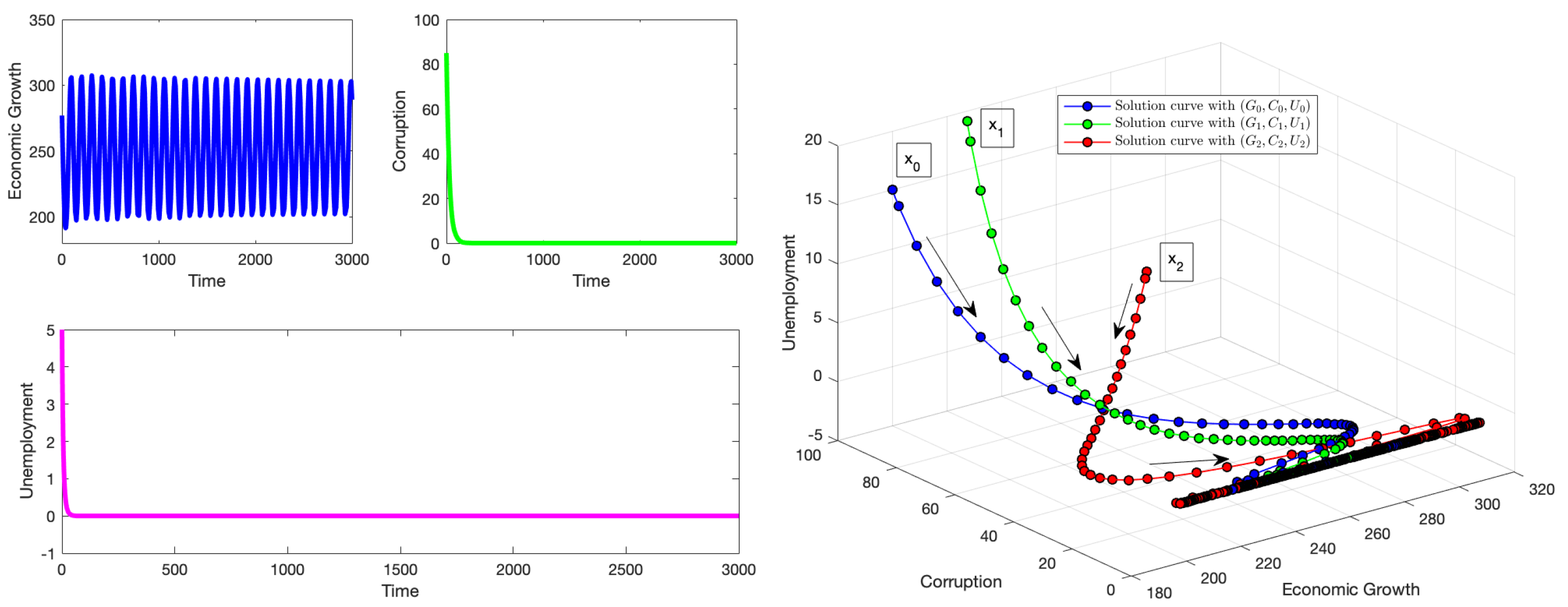
4.1. Simulations for the Equilibrium Point $E_2$

To demonstrate the stability of the equilibrium point $E_2$ and the existence of Hopf bifurcation, we choose parameters $r_1=0.059;,r_2=0.0618,K_1=250,K_2=25,$$\kappa =0.005,$$\beta =0.0001,a=1.25,\varphi =0.77,\mu =0.05,\xi =1/3$. Here, $E_2=(250,0,0)$.

The steady state $E_2$ represents an idealized and perfectly efficient economy where economic growth is at its maximum sustainable level, and there is no corruption and no unemployment, which means that human labor is fully utilized. This equilibrium point reflects the best possible scenario for economic efficiency. However, small perturbations or shocks to the system (such as increases in corruption or unemployment) could destabilize the system, leading to lower growth and higher unemployment, potentially shifting the system to a new equilibrium [65]. In real life, this does not represent any economy but portrays a theoretical goal for a maximum well-functioning system.

In this scenario, the parameter values satisfy the stability conditions: $\mu =0.05>{\displaystyle \frac{\varphi \beta K_1}{a\beta K_1+1}}$ = 0.0187 and $r_2=0.0618>{\displaystyle \frac{K_2(r_2-\kappa )}{K_1\xi }}=0.01704$. We have proved in Theorem 1 that a Hopf bifurcation occurs for system (2) when $\tau ={\tau }_k,k=0,1,2,3,\dots$. From Equation (10), we have ${\tau }_0={\displaystyle \frac{1}{r_1}}\left({\displaystyle \frac{\pi }{2}}\right)=26.624$, ${\tau }_1={\displaystyle \frac{1}{r_1}}({\displaystyle \frac{\pi }{2}}+2\pi )=133.118$, ${\tau }_2={\displaystyle \frac{1}{r_1}}({\displaystyle \frac{\pi }{2}}+4\pi )=239.613$ and so on. But, we are most interested in the case where $k=0$, that is, ${\tau }_0$. We will show the three cases listed in Theorem 2 for $\tau <{\tau }_0,\tau ={\tau }_0,$ and $\tau >{\tau }_0.$

When $\tau <{\tau }_0$, the system is locally stable at the equilibrium point $E_2$. Thus, for initial conditions starting near $E_2$, the system will converge to $E_2$. Figure 1 shows that the system starts with little oscillations in economic growth (the presence of the delay parameter based on the impact of the previous level of economic growth on the current level) and smooths out over time. The system also approaches a situation without corruption and without unemployment. The influence of the discrete time delay $\tau$ is minimal in this context, which means that the levels of prior economic growth do not have a long-term lasting impact on the system.

Figure 2 shows the numerical solutions when $\tau ={\tau }_0=26.624$ and various initial conditions, which include the history function of economic growth $G\left(t\right)$. System (2) shifts from local stability to instability, leading to periodic oscillations, which represent periods of boom and burst cycles in economic growth. A decline in capital or labor, stagnant technological progression, aging population, global instability, etc., can strain economic growth that affects the economy. Understanding and managing these delays is crucial for policymakers to enforce the right policies, execute them appropriately, ensure stable and sustainable economic growth, and avoid prolonged cycles of growth and decline.

Figure 3 shows the numerical solutions when $\tau ={\tau }_0=30$. A crucial observation here is that system (2) approaches an attractor orbit different from the one obtained when $\tau =26.624$. Thus, the previous orbit becomes unstable, but the new orbit with larger amplitude becomes stable. Again, we see the effect of the time delay on generating the economic limit cycles that are often observed in the real world.

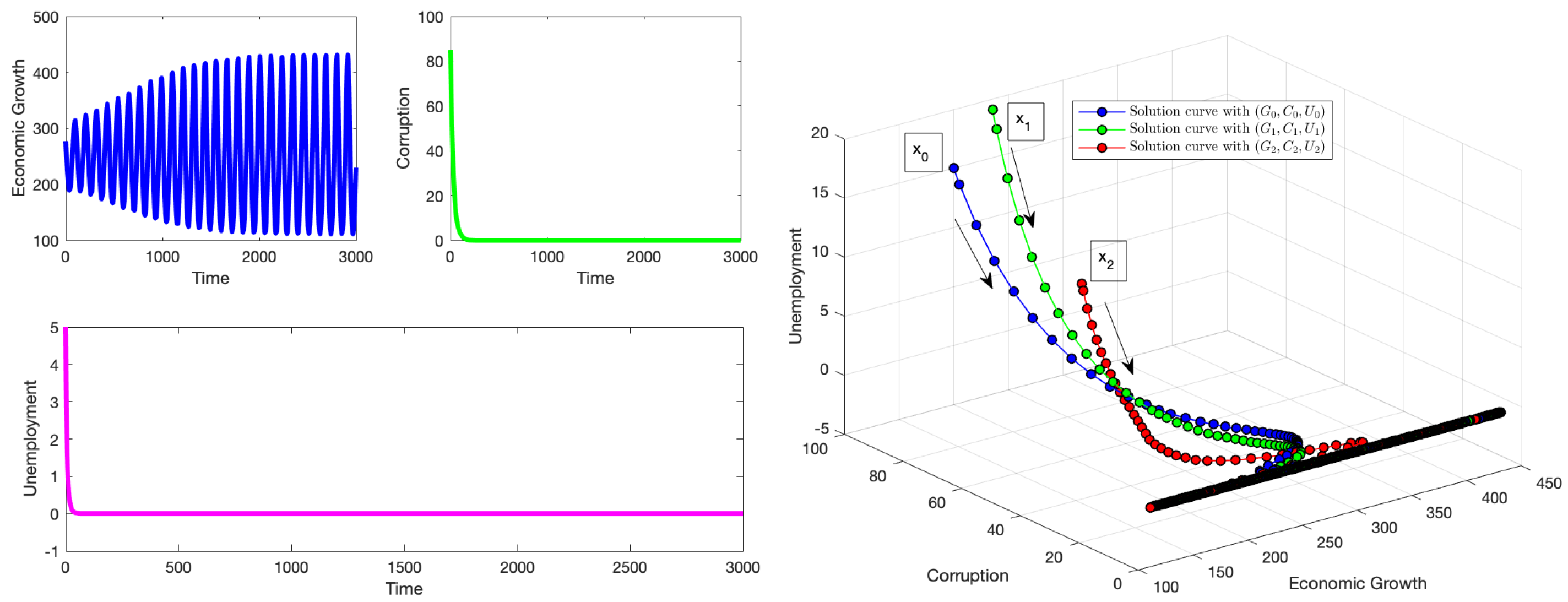
4.2. Simulations for the Equilibrium Point $E_3$

To show the stability of the equilibrium point $E_3$ and the existence of Hopf bifurcations, we choose parameters $r_1=0.029,r_2=0.07,K_1=280,K_2=250,\kappa =0.005,$$\beta =0.001,$$a=0.34,\varphi =0.15,\mu =0.05,\xi =0.4$. With these values, one gets $E_3=(280,0,120.143)$. The equilibrium point $E_3$ represents a state in the economy that grows at its maximum output (since $K_1=280$), corruption is absent, and unemployment is at a moderate level (since $K_2=250$). The carrying capacities for G and U suggest that the system has room for improvement, but it is operating within sustainable limits. The absence of corruption can be interpreted as a highly efficient system where public trust and governance are strong, and economic decisions are made transparently and without undue influence [66].

These parameter values satisfy the local stability conditions: $\mu =0.05>{\displaystyle \frac{\varphi \beta K_1}{a\beta K_1+1}}$ = 0.0383 and $r_2=0.07<{\displaystyle \frac{K_2(r_2-\kappa )}{K_1\xi }}=0.1451$. From Equation (22), we have ${\tau }_0={\displaystyle \frac{1}{r_1}}\left({\displaystyle \frac{\pi }{2}}\right)=54.165$, ${\tau }_1={\displaystyle \frac{1}{r_1}}({\displaystyle \frac{\pi }{2}}+2\pi )=270.827$, ${\tau }_2={\displaystyle \frac{1}{r_1}}({\displaystyle \frac{\pi }{2}}+4\pi )=487.489$, etc. Again, we are most interested in the case where $k=0$, that is, ${\tau }_0$.

We will show numerical simulations of the three cases listed in Theorem (4) for $\tau <{\tau }_0,\tau ={\tau }_0,$ and $\tau >{\tau }_0$. Figure 4 shows the numerical solutions when $\tau =43<{\tau }_0$ and the initial conditions near $E_3$. It can be seen that the value of the delay parameter $\tau$ does not affect the stability of $E_3$ and the long-term behavior of system (2). The solutions converge to $E_3$ as $t\to \infty$. Thus, previous economic growth levels have no effect on the long-term behavior of system (2). Achieving this healthy economic state requires the integration of robust governance, prudent policy frameworks, efficient market mechanisms, strategic investments in human capital, technological advancement, and social inclusion. No single factor can independently ensure these outcomes; rather, it is the harmonious interplay of these elements that fosters an environment conducive to sustainable growth, job creation, and equitable prosperity [67].

Figure 5 shows the numerical solutions when $\tau ={\tau }_0=54.165$ and the initial conditions are relatively close to $E_3$. It can be seen that the value of the delay parameter $\tau$ affects the stability of $E_3$ and the long-term behavior of system (2). Thus, previous economic growth levels have an effect on the long-term behavior of system (2). The solutions converge to an economic limit cycle as $t\to \infty$. In particular, we can see the appearance of a Hopf bifurcation that results when the threshold parameter reaches ${\tau }_0$. The trajectories emerge in a cyclic pattern and oscillate in this fashion for the long term. A Hopf bifurcation in this system striving for optimal economic growth, zero corruption, and a fair unemployment level may occur when the delay of previous economic growth causes feedback loops in the current economic growth. This delay may be due to factors such as delayed policy decisions, market expectations, technological advancements, or labor market dynamics. This shift causes the system to move from a stable equilibrium to one marked by cyclical fluctuations, potentially leading to phases of rapid growth followed by corrective contractions, a direct result of a long-term boom and burst [23,36].

Figure 6 shows the numerical solutions when $\tau ={\tau }_0=60$. Note that system (2) approaches an attractor orbit different from that obtained when $\tau =54.165$. Thus, the previous orbit becomes unstable, but the new orbit with larger amplitude becomes stable. Again, we see the effect of the time delay on generating the economic limit cycles that are often observed in the real world. Under these circumstances, it is apparent that delay levels exceeding the threshold value induce long-term instability of different economic cycles, but stability to a new limit cycle [21,23].

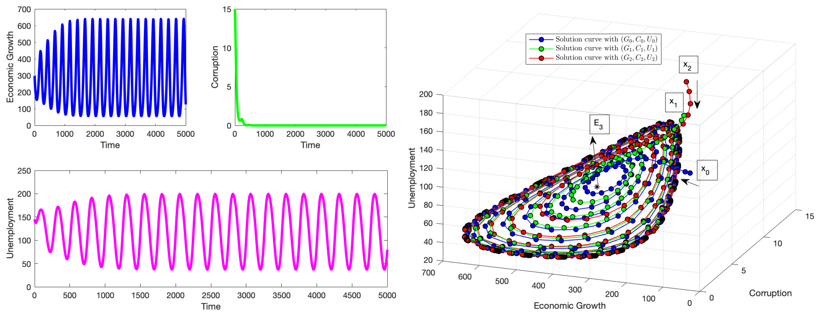
4.3. Simulations for the Equilibrium Point $E_4$

We select parameter values such that all the stability requirements are satisfied. In addition, values for the delay such that the existence of Hopf bifurcation is guaranteed. We perform simulations that verify the theoretical aspect. The parameter values are $r_1=0.99,r_2=0.01,K_1=1250,K_2=570,\kappa =0.21,\beta =0.001,a=0.81,\varphi =0.25,\mu =0.057,$$\xi =0.001$. With these parameters, one gets $E_4=(279.64,942.60,0)$. This steady state $E_4$ represents an economy that operates below its optimal economic output (since $K_1=1250$), with a relatively higher corruption rate and no unemployment. This scenario may arise from a combination of specific economic, political, and social conditions. In this setting, the government can try to avoid unrest by keeping people employed (even in unproductive roles), but overall economic output remains low because corruption, inefficiency, and poor governance dominate the system. The local stability conditions for $E_4$ are satisfied since $r_2=0.01<\kappa +{\displaystyle \frac{r_2\xi G}{K_2}}=0.21,a_1=0.0795>0,a_0=0.0357>0,v_0=0.2922,{\tau }_0=2.9413$. We will show numerical simulations of the three cases listed in Theorem 6 for $\tau <{\tau }_0,\tau ={\tau }_0,$ and $\tau >{\tau }_0$.

Figure 7 shows various numerical solutions with $\tau =2.8<{\tau }_0$. The effect of the delay dissipates over time and does not affect the local stability of $E_4$ and the solutions of system (2) converge to $E_4$ as $t\to \infty$.

Figure 8 shows various numerical solutions with $\tau ={\tau }_0=2.9413$. At this critical value of $\tau$, system (2) undergoes a Hopf bifurcation, in which a pair of conjugate complex eigenvalues transition from the left half of the complex plane ${\mathbb{C}}^{-}$ to the right half plane ${\mathbb{C}}^{+}$, thus shifting system (2) from a stable local steady state to one of instability, characterized by periodic oscillations around the equilibrium point $E_4$ [23]. In this context, the system exhibits sensitivity to delays in economic growth, which propagate throughout the system. The emergence of this Hopf bifurcation may be attributed to nonlinear feedback mechanisms induced by corruption and inefficient economic policies [66]. Upon reaching this critical threshold delay, the system no longer converges to $E_4$, but instead oscillates between alternating phases of elevated and diminished economic output and corruption, thereby manifesting a cyclical economic trajectory.

Figure 9 shows the numerical solutions when $\tau =3>{\tau }_0$. System (2) approaches an attractor orbit different from that obtained when $\tau =2.9413$. Thus, the previous orbit becomes unstable, but the new orbit with larger amplitude becomes stable. Again, we see the effect of the time delay on generating the economic limit cycles that are often observed in the real world.

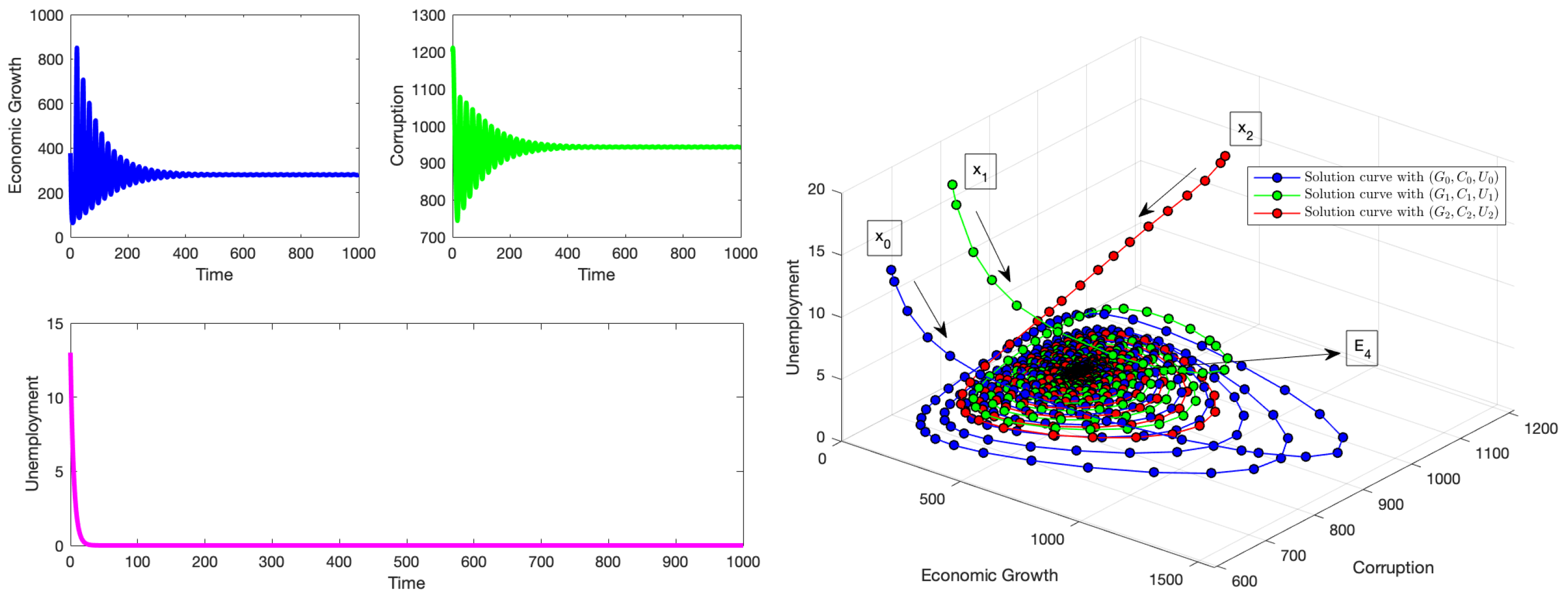
4.4. Simulations for the Equilibrium Point $E_5$

For our last set of simulations, we select the values of the following parameters $r_1=0.25,r_2=0.0118,K_1=550,K_2=125,\kappa =0.003,\beta =0.003,a=0.59,\varphi =0.18,$$\mu =0.01,\xi =0.0$. With these values, one gets $E_5=(19.15,83.16,92.84)$. The equilibrium point $E_5$ signifies an economic state operating below its optimal output, as indicated by the value ($K_1=550$). This scenario is marked by relatively elevated levels of corruption and unemployment, stemming from high rates of economic depletion and subpar economic performance. Numerous underlying factors contribute to this suboptimal outcome. Rampant corruption and ineffective governance impede the efficient allocation of resources, thereby discouraging both domestic and foreign investment, which stymies economic expansion. A range of additional issues, such as political instability, economic dependency, a deficient educational system, an aging population, and a mismatch between available skills and labor market needs, further exacerbate the situation. In addition, the lack of new business ventures, attributable to inadequate governmental support and funding for entrepreneurship, serves as a significant driver of the persistently high unemployment rate within the economy.

In this case, the conditions for local stability are satisfied. In particular, from Theorem (7), one obtains $r_2=0.0118<\kappa +{\displaystyle \frac{r_2(G^{*}\xi +2U^{*})}{K_2}}=0.0206,a_1=0.00079>0,a_0=0.00233>0,$$v_0=0.0502,{\tau }_0=8.579$.

We will numerically explore the three cases listed in Theorem (7) for $\tau <{\tau }_0,\tau ={\tau }_0,$ and $\tau >{\tau }_0$.

Figure 10 shows various numerical solutions with different initial conditions when $\tau ={\tau }_0=7.8$. It can be seen that the effect of the delay on system (2) is fast acting and produces periodic oscillations from the onset that eventually die out and converge to $E_5$ after some time. Solutions starting near $E_5$ converge to $E_5$ as $t\to \infty$. System (2), regarding the interior equilibrium point $E_5$, is sensitive to the time delay in economic growth. An economy characterized by relatively low growth, elevated levels of corruption, and a fair level of unemployment is often a response to the feedback of the delay in previous economic growth characterized by a combination of weak governance, inefficient resource distribution, insufficient investment in innovation, and inadequate infrastructure. The key solution lies in improving economic sustainability, addressing corruption, strengthening governance, promoting innovation, and investing strategically in sectors that can sustain long-term inclusive economic growth [66,68,69].

Figure 11 shows various numerical solutions with $\tau ={\tau }_0=8.579$. At this threshold value of $\tau$, system (2) undergoes a Hopf bifurcation, in which a pair of conjugate complex eigenvalues transition from the left half of the complex plane ${\mathbb{C}}^{-}$ to the right half plane ${\mathbb{C}}^{+}$, thus shifting system (2) from a stable local steady state to one of instability, characterized by periodic oscillations around the equilibrium point $E_5$ [23]. Some factors that may induce this are lag in policy effectiveness, interaction of delayed policy responses, corruption-induced inefficiencies, labor market mismatches, external shocks, weak institutional frameworks, and many more [66,67]. In this scenario, the socioeconomic system (2) is highly sensitive to delays, which requires policymakers to remain proactive and vigilant in crafting and implementing high-quality, timely policies that will steer the economy toward an efficient and sustainable long-term trajectory.

Figure 12 shows the numerical solutions when $\tau =9.5>{\tau }_0$. System (2) approaches an attractor orbit different from that obtained when $\tau =8.579$. Thus, the previous orbit becomes unstable, but the new orbit with larger amplitude becomes stable. In other words, delay levels that surpass this critical delay value cause long-term instability with increasing amplitude levels in the system. Again, we see the effect of the time delay on generating the economic limit cycles that are often observed in the real world.

5. Conclusions

In this article, we extended a socioeconomic mathematical model by incorporating a discrete time delay into the model to account for a more realistic real-world aspect. The model includes the interaction between economic growth, corruption, and unemployment. The time delay is incorporated into the logistic economic growth term in order to take into account the effect of the previous state of the economic growth on its current state. A local stability analysis was performed to investigate the dynamics of the socioeconomic system. Thus, we found conditions where the socioeconomic system will approach different steady states. In addition, we established conditions for the existence of Hopf bifurcations and, therefore, the appearance of economic limit cycles. We found threshold values for the discrete-time delay in which the Hopf bifurcation occurs. We corroborated the theoretical findings by performing numerical simulations for a variety of scenarios. We found various interesting socioeconomic situations where different socioeconomic limit cycles occur. This is important since many socioeconomic cycles occur in the real world. The meaning of the Hopf bifurcations encountered in this work implies that, for some values of the socioeconomic parameters, economic growth, unemployment, and corruption would have oscillations indefinitely unless the values of the parameters change. The parameter values that most significantly affect the emergence of a Hopf bifurcation are those that control the stability of that equilibrium point and influence the imaginary part of the eigenvalues of the system’s Jacobian matrix or characteristic equation. For each equilibrium point, these parameters vary, but in general, for the proposed model, the growth rate plays an important role in the appearance of Hopf bifurcations for all the equilibrium points. To the best of our knowledge, the appearance of limit cycles in mathematical models based on delay differential equations that consider economic growth, corruption, and unemployment has not been reported before. Nevertheless, for a mathematical model without time delay, limit cycles have been found [36]. Moreover, for economic models that consider other economic factors, the appearance of limit cycles has been found [9,27,70]. A future natural extension of this research is to analyze whether additional time delays can be incorporated into the model and investigate whether other types of delay, such as distributed delays, are more realistic. Future works can also study time-varying parameters in the mathematical model, and the analysis would need a very different approach. Furthermore, future work can explore the existence of chaos in the socioeconomic system and also incorporate additional economic factors such as physical capital [71]. One future work that could be very challenging could be to find real-world data to set realistic parameters’ values. For instance, data and measurement regarding corruption could be difficult to gather and analyze. In summary, there are many open avenues of research that can be explored.

References

1. De la Fuente, A.; De La Fuente, A. Mathematical Methods and Models for Economists; Cambridge University Press: Cambridge, UK, 2000. [Google Scholar]
2. Morgan, M.S.; Knuuttila, T. Models and modelling in economics. Philos. Econ. 2012, 13, 49–87. [Google Scholar]
3. Radzicki, M.J. System dynamics and its contribution to economics and economic modeling. In System Dynamics: Theory and Applications; Springer: New York, NY, USA, 2020; pp. 401–415. [Google Scholar]
4. Zhang, W.B. Differential Equations, Bifurcations and Chaos in Economics; World Scientific Publishing Company: Singapore, 2005; Volume 68. [Google Scholar]
5. Feldstein, M.; Horioka, C.; Savings, D. The Solow growth model. Q. J. Econ. 1992, 107, 407–437. [Google Scholar]
6. Nonneman, W.; Vanhoudt, P. A further augmentation of the Solow model and the empirics of economic growth for OECD countries. Q. J. Econ. 1996, 111, 943–953. [Google Scholar] [CrossRef]
7. Solow, R.M. Technical progress, capital formation, and economic growth. Am. Econ. Rev. 1962, 52, 76–86. [Google Scholar]
8. Aniţa, S.; Arnăutu, V.; Capasso, V. An Introduction to Optimal Control Problems in Life Sciences and Economics: From Mathematical Models to Numerical Simulation with MATLAB; Springer Science & Business Media: Berlin/Heidelberg, Germany, 2011. [Google Scholar]
9. Bosi, S.; Desmarchelier, D. Local bifurcations of three and four-dimensional systems: A tractable characterization with economic applications. Math. Soc. Sci. 2019, 97, 38–50. [Google Scholar] [CrossRef]
10. González-Parra, G.; Chen-Charpentier, B.; Arenas, A.J.; Díaz-Rodríguez, M. Mathematical modeling of physical capital diffusion using a spatial Solow model: Application to smuggling in Venezuela. Economies 2022, 10, 164. [Google Scholar] [CrossRef]
11. Ashi, H.; Al-Maalwi, R.M.; Al-Sheikh, S. Study of the unemployment problem by mathematical modeling: Predictions and controls. J. Math. Sociol. 2022, 46, 301–313. [Google Scholar] [CrossRef]
12. Roslan, U.A.M.; Zakaria, S.; Alias, A.; Malik, S. A mathematical model on the dynamics of poverty, poor and crime in West Malaysia. Far. East J. Math. Sci. 2018, 107, 309–319. [Google Scholar] [CrossRef]
13. Buedo-Fernández, S.; Liz, E. On the stability properties of a delay differential neoclassical model of economic growth. Electron. J. Qual. Theory Differ. Equ. 2018, 2018, 1–14. [Google Scholar] [CrossRef]
14. Erman, S. Stability Analysis of Some Dynamic Economic Systems Modeled by State-Dependent Delay Differential Equations. In Global Approaches in Financial Economics, Banking, and Finance; Dincer, H., Hacioglu, Ü., Yüksel, S., Eds.; Springer International Publishing: Cham, Switzerland, 2018; pp. 227–240. [Google Scholar]
15. Matsumoto, A.; Szidarovszky, F. Delay differential nonlinear economic models. In Nonlinear Dynamics in Economics, Finance and Social Sciences: Essays in Honour of John Barkley Rosser Jr; Springer: Berlin/Heidelberg, Germany, 2009; pp. 195–214. [Google Scholar]
16. Ruzgas, T.; Jankauskienė, I.; Zajančkauskas, A.; Lukauskas, M.; Bazilevičius, M.; Kaluževičiūtė, R.; Arnastauskaitė, J. Solving Linear and Nonlinear Delayed Differential Equations Using the Lambert W Function for Economic and Biological Problems. Mathematics 2024, 12, 2760. [Google Scholar] [CrossRef]
17. Segura, J.; Franco, D.; Perán, J. Long-run economic growth in the delay spatial Solow model. Spat. Econ. Anal. 2023, 18, 158–172. [Google Scholar] [CrossRef]
18. Rajpal, A.; Bhatia, S.K.; Goel, S.; Kumar, P. Time delays in skill development and vacancy creation: Effects on unemployment through mathematical modelling. Commun. Nonlinear Sci. Numer. Simul. 2024, 130, 107758. [Google Scholar] [CrossRef]
19. Çalış, Y.; Demirci, A.; Özemir, C. Hopf bifurcation of a financial dynamical system with delay. Math. Comput. Simul. 2022, 201, 343–361. [Google Scholar] [CrossRef]
20. Özbay, H.; Sağlam, H.Ç.; Yüksel, M.K. Hopf cycles in one-sector optimal growth models with time delay. Macroecon. Dyn. 2017, 21, 1887–1901. [Google Scholar] [CrossRef]
21. Guckenheimer, J.; Holmes, P. Nonlinear Oscillations, Dynamical Systems, and Bifurcations of Vector Fields; Springer Science & Business Media: Berlin/Heidelberg, Germany, 2013; Volume 42. [Google Scholar]
22. Hirsch, M.W.; Smale, S.; Devaney, R.L. Differential Equations, Dynamical Systems, and an Introduction to Chaos; Academic Press: New York, NY, USA, 2013. [Google Scholar]
23. Marsden, J.E.; McCracken, M. The Hopf Bifurcation and Its Applications; Springer Science & Business Media: Berlin/Heidelberg, Germany, 2012; Volume 19. [Google Scholar]
24. Al-Hdaibat, B. Computational Dynamical Systems Analysis: Bogdanov-Takens Points and an Economic Model. Ph.D. Thesis, Ghent University, Ghent, Belgium, 2015. [Google Scholar]
25. Krawiec, A.; Szydłowski, M. Economic growth cycles driven by investment delay. Econ. Model. 2017, 67, 175–183. [Google Scholar] [CrossRef]
26. Manfredi, P.; Fanti, L. Cycles in dynamic economic modelling. Econ. Model. 2004, 21, 573–594. [Google Scholar] [CrossRef]
27. Pribylova, L. Bifurcation routes to chaos in an extended Van der Pol’s equation applied to economic models. Electron. J. Differ. Equ. (EJDE) 2009, 2009, 1–21. [Google Scholar]
28. Dockner, E.J.; Feichtinger, G. On the optimality of limit cycles in dynamic economic systems. J. Econ. 1991, 53, 31–50. [Google Scholar] [CrossRef]
29. Feichtinger, G. Limit cycles in dynamic economic systems. Ann. Oper. Res. 1992, 37, 313–344. [Google Scholar] [CrossRef]
30. Feichtinger, G.; Novak, A.; Wirl, F. Limit cycles in intertemporal adjustment models: Theory and applications. J. Econ. Dyn. Control 1994, 18, 353–380. [Google Scholar] [CrossRef]
31. Kryuchkov, V.; Solomonovich, M.; Anton, C. Moving limit cycles model of an economic system. In Proceedings of the Numerical Analysis and Its Applications: 6th International Conference, NAA 2016, Lozenetz, Bulgaria, 15–22 June 2016; Revised Selected Papers 6. Springer: Berlin/Heidelberg, Germany, 2017; pp. 456–463. [Google Scholar]
32. Markakis, M.; Douris, P. Stability and analytical approximation of limit cycles in Hopf bifurcations of four-dimensional economic models. Appl. Math. Sci. 2014, 8, 3697–3990. [Google Scholar] [CrossRef]
33. Araujo, R.A.; Flaschel, P.; Moreira, H.N. Limit cycles in a model of supply-side liquidity/profit-rate in the presence of a Phillips curve. Economia 2020, 21, 145–159. [Google Scholar] [CrossRef]
34. Asada, T.; Demetrian, M.; Zimka, R. The stability of normal equilibrium point and the existence of limit cycles in a simple Keynesian macrodynamic model of monetary policy. In Essays in Economic Dynamics: Theory, Simulation Analysis, and Methodological Study; Springer: Singapore, 2016; pp. 145–162. [Google Scholar]
35. Bazán Navarro, C.E.; Benazic Tomé, R.M. Structural Stability Analysis in a Dynamic IS-LM-AS Macroeconomic Model with Inflation Expectations. Int. J. Differ. Equ. 2022, 2022, 5026061. [Google Scholar] [CrossRef]
36. Ifeacho, O.; González-Parra, G. Hopf Bifurcations in a Mathematical Model for Economic Growth, Corruption, and Unemployment: Computation of Economic Limit Cycles. Axioms 2025, 14, 173. [Google Scholar] [CrossRef]
37. Anderson, R.M.; Jackson, H.C.; May, R.M.; Smith, A.M. Population dynamics of fox rabies in Europe. Nature 1981, 289, 765–771. [Google Scholar] [CrossRef]
38. Greenhalgh, D. Hopf bifurcation in epidemic models with a latent period and nonpermanent immunity. Math. Comput. Model. 1997, 25, 85–107. [Google Scholar] [CrossRef]
39. Sepulveda, G.; Arenas, A.J.; González-Parra, G. Mathematical modeling of COVID-19 dynamics under two vaccination doses and delay effects. Mathematics 2023, 11, 369. [Google Scholar] [CrossRef]
40. Baráková, L. Asymptotic Behaviour and Hopf Bifurcation of a Three-Dimensional Nonlinear Autonomous System. Georgian Math. J. 2002, 9, 207–226. [Google Scholar] [CrossRef]
41. Ifeacho, O.; González-Parra, G. Mathematical Modeling of Economic Growth, Corruption, Employment and Inflation. Mathematics 2025, 13, 1102. [Google Scholar] [CrossRef]
42. Callen, T. Gross Domestic Product: An Economy’s All; International Monetary Fund: Washington, DC, USA, 2012. [Google Scholar]
43. McCusker, J.J. Estimating early American gross domestic product. Hist. Methods J. Quant. Interdiscip. Hist. 2000, 33, 155–162. [Google Scholar] [CrossRef]
44. Belda Mullor, G. Citizens’ Attitude Towards Political Corruption and the Impact of Social Media. Ph.D. Thesis, Universitat Jaume I, Castellón de la Plana, Spain, 2018. [Google Scholar]
45. Dritsaki, C.; Dritsaki, M. Phillips curve inflation and unemployment: An empirical research for Greece. Int. J. Comput. Econ. Econom. 2013, 3, 27–42. [Google Scholar] [CrossRef]
46. Flaschel, P.; Landesmann, M. Mathematical Economics and the Dynamics of Capitalism: Goodwin’s Legacy Continued; Routledge: London, UK, 2016. [Google Scholar]
47. Ho, S.Y.; Iyke, B.N. Unemployment and inflation: Evidence of a nonlinear Phillips curve in the Eurozone. J. Dev. Areas 2019, 53, 151–163. [Google Scholar] [CrossRef]
48. Ormerod, P.; Rosewell, B.; Phelps, P. Inflation/unemployment regimes and the instability of the Phillips curve. Appl. Econ. 2013, 45, 1519–1531. [Google Scholar] [CrossRef]
49. Ravenna, F.; Walsh, C.E. Vacancies, unemployment, and the Phillips curve. Eur. Econ. Rev. 2008, 52, 1494–1521. [Google Scholar] [CrossRef]
50. Calmfors, L.; Holmlund, B. Unemployment and economic growth: A partial survey. Swed. Econ. Policy Rev. 2000, 7, 107–154. [Google Scholar]
51. Jibir, A.; Bappayaya, B.; Babayo, H. Re-examination of the impact of unemployment on economic growth of Nigeria: An econometric approach. J. Econ. Sustain. Dev. 2015, 6, 116–123. [Google Scholar]
52. Sekwati, D.; Dagume, M.A. Effect of unemployment and inflation on economic growth in South Africa. Int. J. Econ. Financ. Issues 2023, 13, 35–45. [Google Scholar] [CrossRef]
53. Alfifi, H.Y. Stability and Hopf bifurcation analysis for the diffusive delay logistic population model with spatially heterogeneous environment. Appl. Math. Comput. 2021, 408, 126362. [Google Scholar] [CrossRef]
54. Bianca, C.; Guerrini, L. On the Dalgaard-Strulik model with logistic population growth rate and delayed-carrying capacity. Acta Appl. Math. 2013, 128, 39–48. [Google Scholar] [CrossRef]
55. Bianca, C.; Guerrini, L. Existence of limit cycles in the Solow Model with delayed-logistic population growth. Sci. World J. 2014, 2014, 207806. [Google Scholar] [CrossRef]
56. ElFadily, S.; Khalid, N.; Kaddar, A. Stability Analysis of Bifurcated Limit Cycles in a Labor Force Evolution Model. In The International Congress of the Moroccan Society of Applied Mathematics; Springer: Cham, Switzerland, 2019; pp. 61–77. [Google Scholar]
57. Xu, R.; Wang, Z.; Zhang, F. Global stability and Hopf bifurcations of an SEIR epidemiological model with logistic growth and time delay. Appl. Math. Comput. 2015, 269, 332–342. [Google Scholar] [CrossRef]
58. Mamo, D.K.; Ayele, E.A.; Teklu, S.W. Modelling and Analysis of the Impact of Corruption on Economic Growth and Unemployment. In Operations Research Forum; Springer: Cham, Switzerland, 2024; Volume 5, p. 36. [Google Scholar]
59. Hale, J.K.; Verduyn Lunel, S.M. Introduction to Functional Differential Equations; Springer: New York, NY, USA, 1993; Volume 99. [Google Scholar] [CrossRef]
60. Kuang, Y. Delay Differential Equations; Academic Press: New York, NY, USA, 1993. [Google Scholar]
61. Gopalsamy, K. Stability and Oscillations in Delay Differential Equations of Population Dynamics; Springer Science & Business Media: Berlin/Heidelberg, Germany, 2013; Volume 74. [Google Scholar]
62. Breda, D.; Maset, S.; Vermiglio, R. Stability of Linear Delay Differential Equations: A Numerical Approach with MATLAB; Springer: Berlin/Heidelberg, Germany, 2014. [Google Scholar]
63. Shampine, L.F.; Thompson, S. Solving ddes in matlab. Appl. Numer. Math. 2001, 37, 441–458. [Google Scholar] [CrossRef]
64. Shampine, L.F.; Thompson, S. Numerical Solution of Delay Differential Equations. In Delay Differential Equations; Springer: Boston, MA, USA, 2009; pp. 1–27. [Google Scholar]
65. Jones, L.E.; Manuelli, R.E. A model of Optimal Equilibrium Growth; Graduate School of Business, Stanford University: Stanford, CA, USA, 1988. [Google Scholar]
66. Mauro, P. Corruption and growth. Q. J. Econ. 1995, 110, 681–712. [Google Scholar] [CrossRef]
67. Acemoglu, D.; Robinson, J. The Role of Institutions in Growth and Development; World Bank: Washington, DC, USA, 2008; Volume 10. [Google Scholar]
68. Uddin, I.; Rahman, K.U. Impact of corruption, unemployment and inflation on economic growth evidence from developing countries. Qual. Quant. 2023, 57, 2759–2779. [Google Scholar] [CrossRef]
69. Triatmanto, B.; Bawono, S. The interplay of corruption, human capital, and unemployment in Indonesia: Implications for economic development. J. Econ. Criminol. 2023, 2, 100031. [Google Scholar] [CrossRef]
70. Moza, G.; Rocşoreanu, C.; Sterpu, M.; Oliveira, R. Stability and bifurcation analysis of a four-dimensional economic model. Carpathian J. Math. 2024, 40, 139–153. [Google Scholar] [CrossRef]
71. Fernández-Díaz, A. Overview and perspectives of chaos theory and its applications in economics. Mathematics 2023, 12, 92. [Google Scholar] [CrossRef]
Figure 1. For τ = 20 < τ 0 . Dynamics of system (2) with initial condition x 2 = ( 277 , 85 , 5 ) (left). Phase-space plot of system (2) with initial conditions x 0 = ( 200 , 100 , 15 ) , x 1 = ( 222 , 95 , 20 ) , x 2 = ( 277 , 85 , 5 ) (right).
Appliedmath 05 00057 g001
Figure 2. For τ = τ 0 = 26.624 . Dynamics of system (2) with initial condition x 2 = ( 277 , 85 , 5 ) (left). Phase-space plot of system (2) with initial conditions x 0 = ( 200 , 100 , 15 ) , x 1 = ( 222 , 95 , 20 ) , x 2 = ( 277 , 85 , 5 ) (right).
Appliedmath 05 00057 g002
Figure 3. For τ = 30 > τ 0 . Dynamics of system (2) with initial condition x 2 = ( 277 , 85 , 5 ) (left). Phase-space plot of system (2) with initial conditions x 0 = ( 200 , 100 , 15 ) , x 1 = ( 222 , 95 , 20 ) , x 2 = ( 277 , 85 , 5 ) (right).
Appliedmath 05 00057 g003
Figure 4. For τ = 43 < τ 0 and E 3 = ( 280 , 0 , 120.143 ) . Dynamics of system (2) with initial condition x 2 = ( 297 , 15 , 145 ) (left). Phase plot of the system with initial conditions x 0 = ( 200 , 10 , 80 ) , x 1 = ( 252 , 12 , 128 ) , x 2 = ( 297 , 15 , 145 ) (right).
Appliedmath 05 00057 g004
Figure 5. For τ = τ 0 = 54.165 . Dynamics of system (2) with initial condition x 2 = ( 297 , 15 , 145 ) (left). Phase plot of the system with initial conditions x 0 = ( 200 , 10 , 80 ) , x 1 = ( 252 , 12 , 128 ) , x 2 = ( 297 , 15 , 145 ) (right).
Appliedmath 05 00057 g005
Figure 6. For τ = 60 > τ 0 . Dynamics of system (2) with initial condition x 2 = ( 297 , 15 , 145 ) (left). Phase plot of the system with initial conditions x 0 = ( 200 , 10 , 80 ) , x 1 = ( 252 , 12 , 128 ) , x 2 = ( 297 , 15 , 145 ) (right).
Appliedmath 05 00057 g006
Figure 7. For τ = 2.8 < τ 0 and E 4 = ( 279.64 , 942.60 , 0 ) . Dynamics of system (2) with initial condition x * = ( 377 , 1200 , 13 ) (left). Phase plot of the system with initial conditions x 0 = ( 200 , 600 , 15 ) , x 1 = ( 242 , 705 , 20 ) , x 2 = ( 377 , 1200 , 15 ) (right).
Appliedmath 05 00057 g007
Figure 8. For τ = τ 0 = 2.9413 . Dynamics of system (2) with initial condition x * = ( 377 , 1200 , 13 ) (left). Phase plot of the system with initial conditions x 0 = ( 200 , 600 , 15 ) , x 1 = ( 242 , 705 , 20 ) , x 2 = ( 377 , 1200 , 15 ) (right).
Appliedmath 05 00057 g008
Figure 9. For τ = 3 > τ 0 . Dynamics of system (2) with initial condition x * = ( 377 , 1200 , 13 ) (left). Phase plot of the system with initial conditions x 0 = ( 200 , 600 , 15 ) , x 1 = ( 242 , 705 , 20 ) , x 2 = ( 377 , 1200 , 15 ) (right).
Appliedmath 05 00057 g009
Figure 10. For τ = 7.8 < τ 0 . Dynamics of system (2) with initial condition x 2 = ( 27 , 100 , 94 ) (left). Phase plot of the system with initial conditions x 0 = ( 12 , 67 , 55 ) , x 1 = ( 14 , 75 , 72 ) , x 2 = ( 27 , 100 , 94 ) (right).
Appliedmath 05 00057 g010
Figure 11. For τ = τ 0 = 8.579 . Dynamics of system (2) with initial condition x 2 = ( 27 , 100 , 94 ) (left). Phase plot of the system with initial conditions x 0 = ( 12 , 67 , 55 ) , x 1 = ( 14 , 75 , 72 ) , x 2 = ( 27 , 100 , 94 ) (right).
Appliedmath 05 00057 g011
Figure 12. For τ = 9.5 > τ 0 . Dynamics of system (2) with initial condition x 2 = ( 27 , 100 , 94 ) (left). Phase plot of the system with initial conditions x 0 = ( 12 , 67 , 55 ) , x 1 = ( 14 , 75 , 72 ) , x 2 = ( 27 , 100 , 94 ) (right).
Appliedmath 05 00057 g012