Abstract
The method of particular solutions using polynomial basis functions (MPS-PBF) has been extensively used to solve various types of partial differential equations. Traditional methods employing radial basis functions (RBFs)—such as Gaussian, multiquadric, and Matérn functions—often suffer from accuracy issues due to their dependence on a shape parameter, which is very difficult to select optimally. In this study, we adopt the MPS-PBF to solve the time-dependent Schrödinger equation in two dimensions. By utilizing polynomial basis functions, our approach eliminates the need to determine a shape parameter, thereby simplifying the solution process. Spatial discretization is performed using the MPS-PBF, while temporal discretization is handled via the backward Euler and Crank–Nicolson methods. To address the ill conditioning of the resulting system matrix, we incorporate a multi-scale technique. To validate the efficacy of the proposed scheme, we present four numerical examples and compare the results with known analytical solutions, demonstrating the accuracy and robustness of the scheme.
1. Introduction
The Schrödinger equation is a partial differential equation (PDE) that governs the wave function of a non-relativistic quantum-mechanical system [1]. The time-dependent Schrödinger equation has been widely used in the field of quantum mechanics such as modeling of quantum devices, electromagnetic wave propagation, underwater acoustics, and the design of certain optoelectronic devices since it models an electromagnetic wave equation given by the potential function [2,3,4,5].
In the literature, many researchers have successfully employed various mesh-based and meshless numerical methods for solving the Schrödinger equation in multiple dimensions. The finite difference method, a well-known mesh-based method, has been used for the numerical solution of the 2D Schrödinger equation [6,7]. While solving time-dependent problems, Feng et al. proposed a compact finite difference scheme for solving the time-fractional Black Scholes option pricing model [8]. Similarly, Zhang et al. proposed a local discontinuous Galerkin (LDG) method for solving a fourth-order time fractional sub-diffusion model [9]. Dehghan et al. implemented a meshless numerical method for the 2D Schrödinger equation using the radial basis function (RBF) collocation method [10]. Montegranario et al. applied a meshless method using multiquadric RBFs for solving the one- and two-dimensional time-dependent Schrödinger equations [11]. More recently, Elgharbi et al. utilized the Sinc collocation method and double exponential transformations for solving the 2D time-dependent Schrödinger equation [12].
When implementing meshless methods using RBFs, the selection of optimal shape parameter is a challenging task for researchers in this field. Therefore, researchers have employed various numerical methods using basis functions which do not use a shape parameter in the solution process. One well-known numerical scheme which does not utilize a shape parameter is the method of particular solutions using polynomial basis functions (MPS-PBF). This approach is proven to be more accurate and easy to implement due to the availability of close-form particular solutions for general linear second-order differential equations. Dangal et al. employed the MPS-PBF for solving different types of partial differential equations [13]. Since Schrödinger’s equations have been used for decades to model various problems that arise in the field of quantum mechanics, we develop a numerical scheme using the MPS-PBF for solving time-dependent Schrödinger equations in this article.
The structure of the remaining content is as follows: Section 2 details the solution methodology of our numerical scheme using the MPS-PBF for solving time-dependent Schrödinger equations in 2D. Numerical examples and the results are discussed in Section 3. Conclusions and future work are provided in Section 4.
2. Solution Methodology
2.1. Time Discretization of the Schrödinger Equation
Consider the following two-dimensional time-dependent Schrödinger equation,
with the initial condition
the Dirichlet boundary condition
and the Neumann boundary condition
where is the unit outward normal vector at the boundary and , , , and are known functions. Here, describes the potential energy of a particle on its domain.
The and denote the boundaries on which the Dirichlet and Neumann conditions are applied, respectively, such that the total boundary is denoted as ,
Let us discretize Equation (1) in the time domain using a -weighted scheme as follows:
Let us set and . Then, in each time step, , , Equation (5) becomes
2.2. Polynomial Basis Functions
The sequence of polynomials
forms a basis for polynomials of a degree less than or equal to r in two variables. Here, gives the dimension of the polynomial basis function space. The particular solutions of the polynomial basis functions are required in the method of particular solutions. Dangal et al. [13] derived the closed-form particular solutions of monomials for a general linear second-order partial differential operator with constant coefficients.
Consider a general form of second-order linear partial differential equations in two variables with constant coefficients:
where the coefficients are real constants, , and i and j are positive integers. Then, the particular solution in Equation (8) is given by
where and
2.3. Numerical Discretization of Schrödinger Equation Using MPS-PBF
Suppose a domain in has interior nodes and boundary nodes such that total number of collocation nodes is The method of particular solution approximates the solution of a partial differential equation as a linear combination of particular solutions of the polynomial basis functions in each time step, , , as follows:
where
The system of Equations (15)–(18) can be written in matrix form as follows:
where , , , is a zero matrix of the size and represent the right-hand side of Equations (15)–(18), respectively. The approximate solutions can be computed from Equation (10) once the unknown coefficients and are recovered from the matrix Equation (19). In this paper, we use the proposed numerical scheme with and for our numerical experiments.
2.4. Multiple-Scale Technique
In the numerical experiments, we employed polynomial basis functions of a higher order to achieve considerable accuracy. The MPS-PBF produced a highly ill-conditioned matrix when we increased the order of the polynomial basis functions. To address this issue, we employed the multiple-scale technique [14] which effectively reduced the condition number of the resultant matrix due to which highly accurate and stable numerical results were obtained. In the multiple-scale technique, each column of the resultant matrix was normalized and we solved a new system of equations and recovered unknown coefficients, and .
3. Numerical Results
In this section, we present four numerical examples to verify the effectiveness of our proposed numerical scheme. The numerical accuracy of the solutions were measured by the root mean square error (RMSE) and maximum absolute error () which are defined as follows:
and
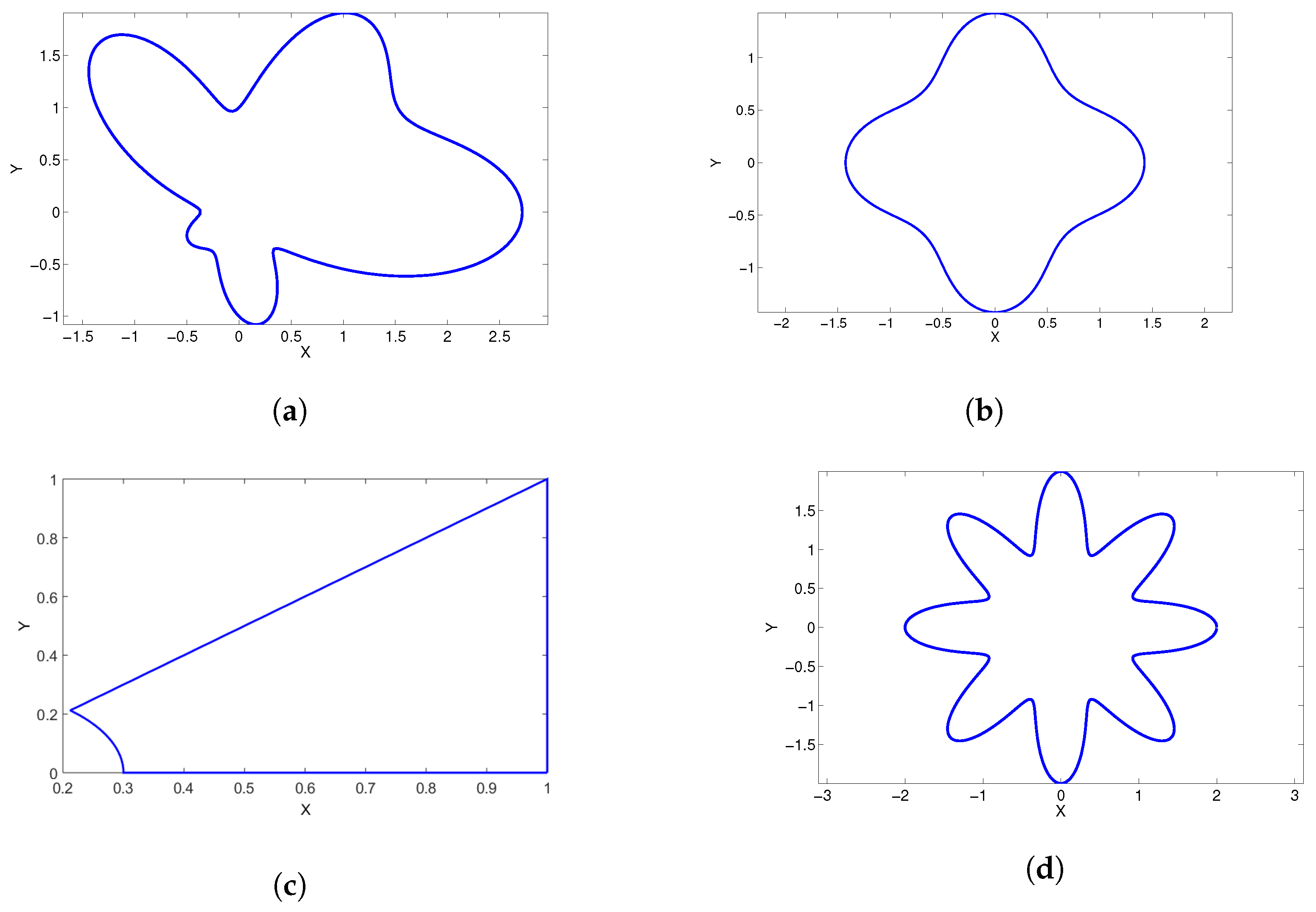
In most of our numerical experiments, we used the order of polynomial basis functions of 13 unless otherwise stated. The profile of boundaries of computational domains under consideration are given in Figure 1.
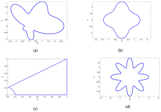
Figure 1.
Computational domains. (a) Amoeba-shaped. (b) Cassini-shaped. (c) Corner-shaped. (d) Star-shaped.
Example 1.


In this example, we solve the Schrödinger Equations (1)–(3) with the potential function,
where and g are given based on the following analytical solution:
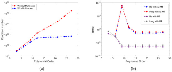
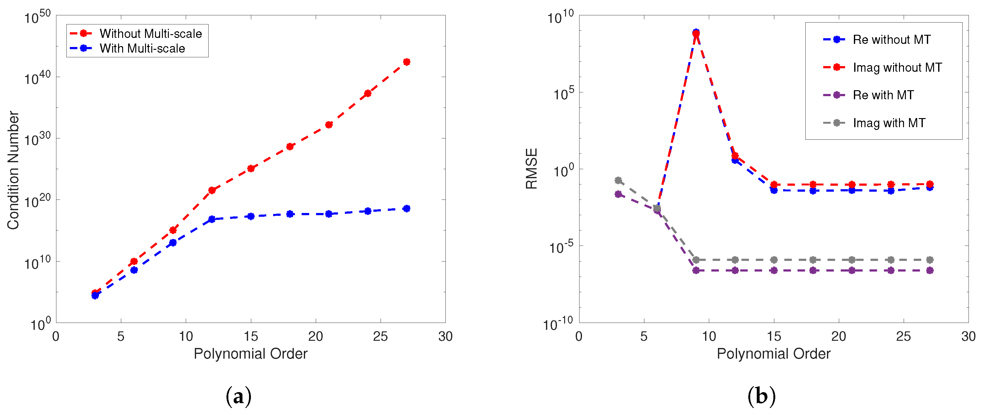
We first chose interior nodes and boundary nodes on a corner-shaped (Figure 1c) computational domain. The Crank–Nicolson scheme was applied for temporal discretization with a time step of and a terminal time of for this experiment. Figure 2a illustrates the effect of the multiple-scale technique which significantly reduced the condition number of the resultant matrix. The multiple-scale technique played a crucial role in achieving highly accurate and stable results, particularly as the order of polynomial basis functions increased. As shown in Figure 2b, the accuracy of the method improved from 1 × 10⁻² to 1 × 10⁻⁷ with the implementation of the multiple-scale technique.
Figure 2.
Example 1: Profiles of polynomial orders versus condition number (a) and polynomial orders versus RMSE (b).
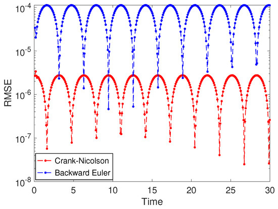
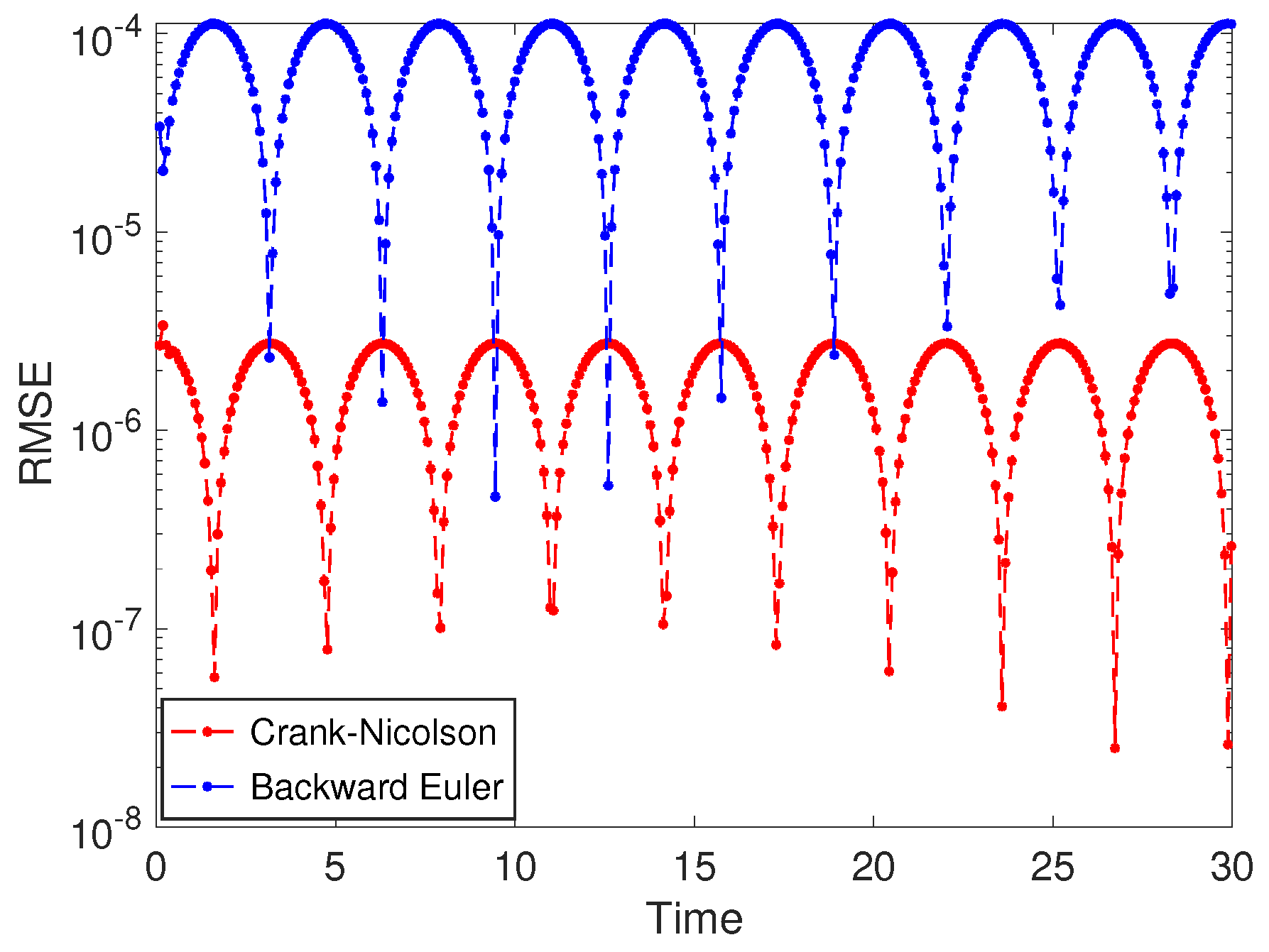
Furthermore, we performed a comparison between two temporal discretization techniques, the backward Euler method and the Crank–Nicolson method, on a unit square domain to verify the effectiveness of our method. We compared the RMSE of the real parts of the solution for both methods in which the computational domain consisted of interior nodes and boundary nodes. We selected a time step of , polynomial basis functions of the order 13, and a terminal time for this experiment. As shown in Figure 3, both methods yielded stable and highly accurate solutions over the time interval . The comparison clearly demonstrates the effectiveness of the proposed method.
Figure 3.
Example 1: Profiles of RMSEs with two time discretization techniques, Crank–Nicolson and backward Euler methods.
The numerical accuracy of the collocation methods using radial basis functions such as multiquadric functions () heavily depends on the shape parameter c. However, we do not need a shape parameter for the MPS-PBF. The comparison of the numerical accuracy between the RBF collocation method and MPS-PBF is presented in Table 1. The numerical results for the multiquadric (MQ) radial basis function are taken from the article by Dehghan et al. [10]. In this comparison, polynomial basis functions of the order 13 were employed with the time step chosen on a unit square domain. The results clearly indicate that the MPS-PBF provided significantly more accurate solutions than the MQ RBF at various terminal times, . An important advantage of the MPS-PBF is that it avoids the use of an indeterminant shape parameter, which is a major challenge in many RBF collocation methods.
Table 1.
Example 1: Comparison of maximum absolute errors between collocation method using radial basis function and polynomial basis functions.
Next, we present the numerical accuracy of the proposed method with different time steps. Table 2 presents a comparison of the error estimate for the real and imaginary parts of the solution to the given problem, evaluated for various time steps using the backward Euler method and Crank–Nicolson method. The numerical results in the table clearly demonstrate that both methods are very stable and highly accurate.
Table 2.
Example 1: Comparison of RMSEs between two temporal discretization techniques for various time steps at terminal time .
Additionally, we investigated the performance of our method for various terminal times, ranging from to The numerical results presented in Table 3 further confirm that both the backward Euler method and Crank–Nicolson method yielded highly accurate and stable results across the different terminal times.
Table 3.
Example 1: Comparison of RMSEs between two temporal discretization techniques for various terminal times.
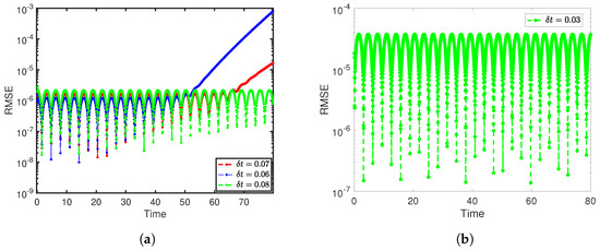
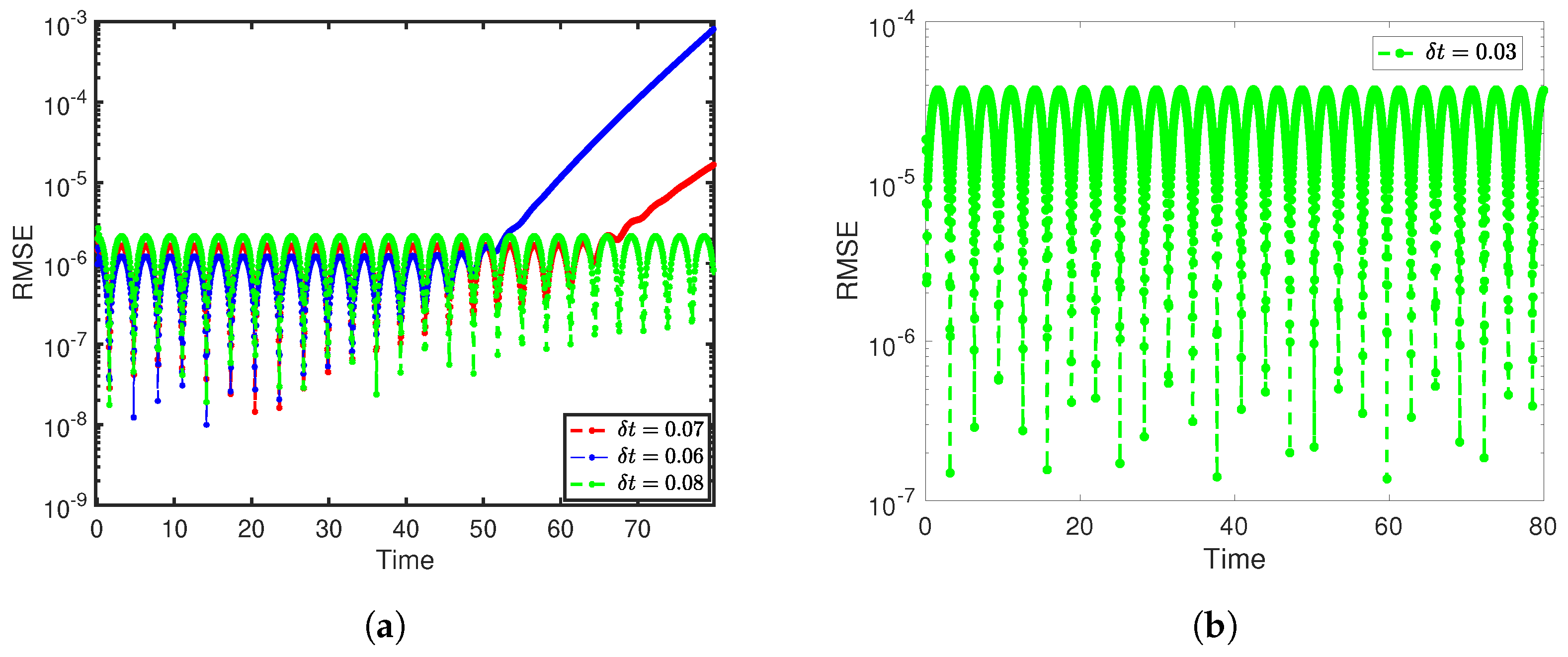
Figure 4a displays the RMSE versus terminal time for different time steps (, 0.07, 0.08) using the Crank–Nicolson method. In this method, larger time steps were generally required to achieve better accuracy for higher terminal times. However, accuracy began to deteriorate beyond a certain terminal time, as depicted in the Figure 4a. On the other hand, Figure 4b exhibits the RMSE versus terminal time for a fixed time step, , and terminal time, , using the backward Euler method. Unlike the Crank–Nicolson method, the backward Euler method provided stable numerical results even with smaller time steps, maintaining accuracy for higher terminal times. From the Figure 4, we observe that both methods produced highly accurate numerical results but the Crank–Nicolson method demonstrated superior numerical accuracy compared to the backward Euler method.
Figure 4.
Example 1: RMSEs for various time steps with Crank–Nicolson method (a) and RMSEs for using backward Euler method (b). (a) RMSE vs. time. (b) RMSE vs. time.
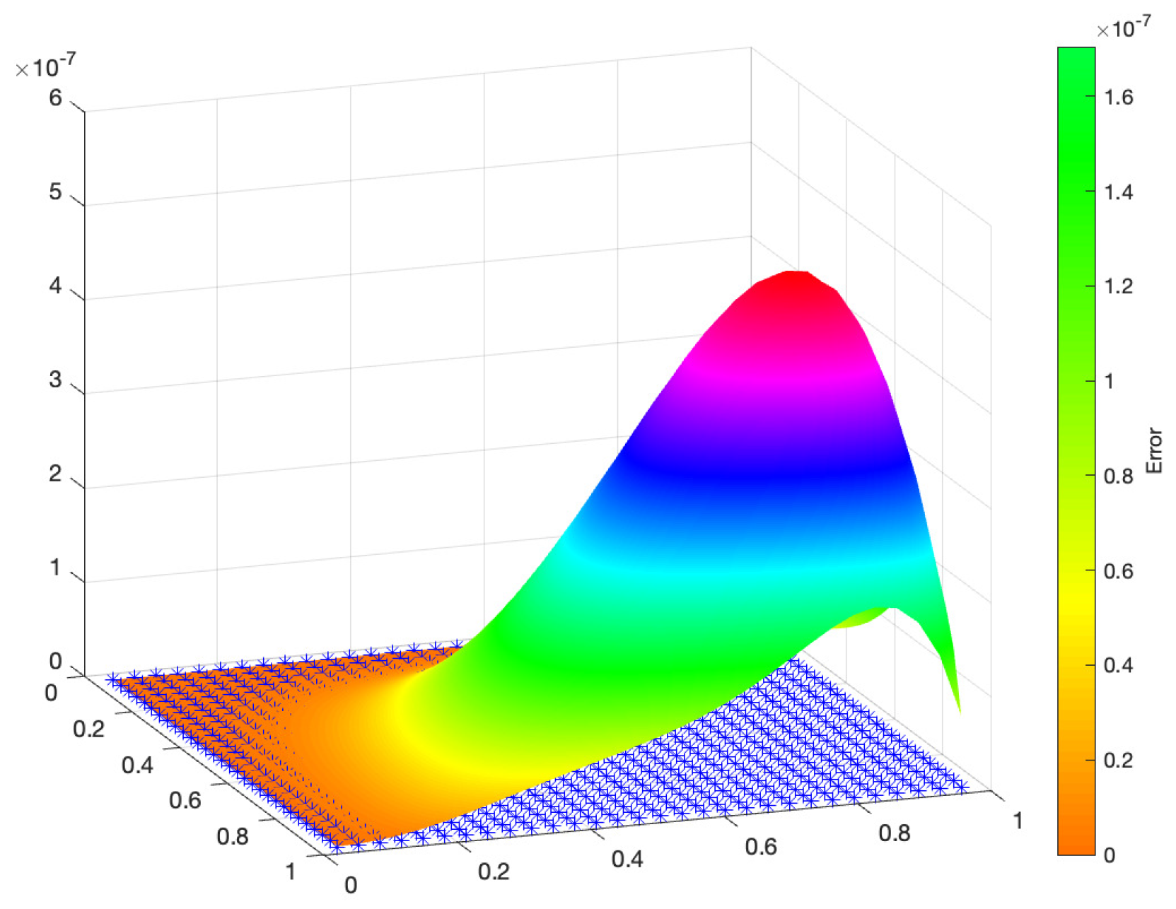
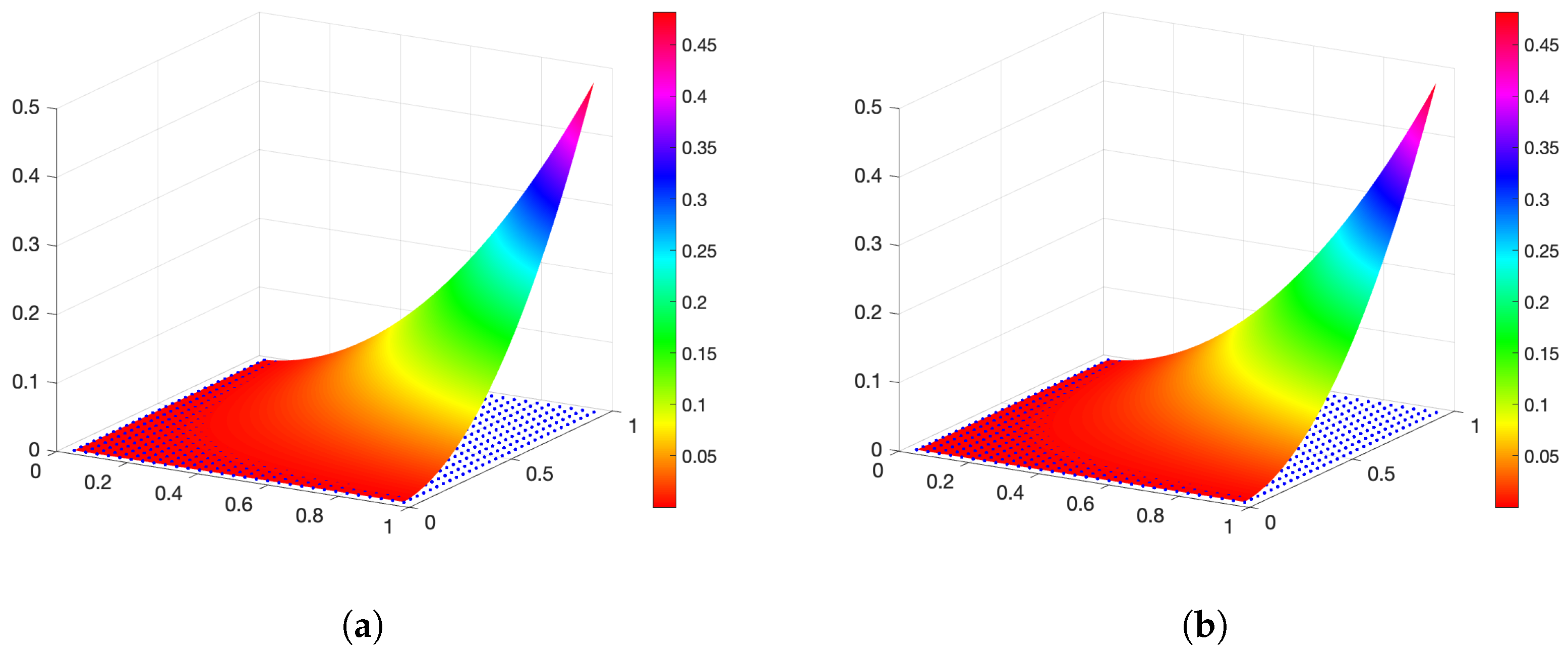
Figure 5 illustrates the absolute value error distribution on the surface of the domain, while Figure 6 displays the approximate and exact solutions for the real part of the solution. This experiment was conducted using the Crank–Nicolson method with a time step of and a terminal time of The computational domain consisted of 900 interior nodes and 236 boundary nodes. From Figure 5, we observe that error was maximized in regions where the solution exhibited a higher gradient which aligned with our expectations.
Figure 5.
Example 1: Distribution of absolute value errors on unit square domain.
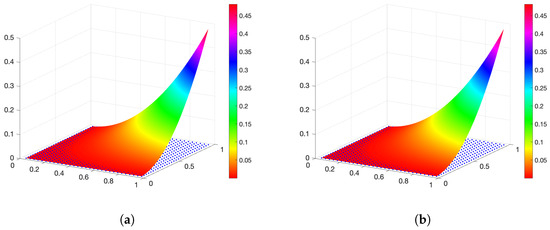
Figure 6.
Example 1: (a) Approximate solutions. (b) Exact solutions.
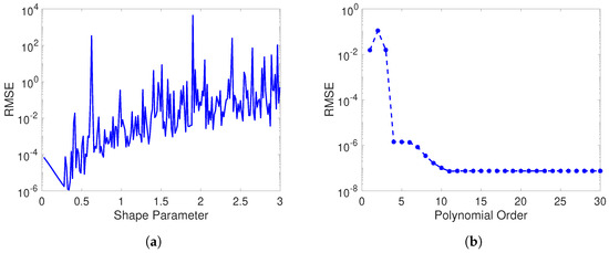
Now, we describe how we solved this equation for the imaginary part of the solution on a unit square domain using an MPS based on multiquadric radial basis function (MPS-RBF) and polynomial basis functions (MPS-PBF). The numbers of interior nodes and boundary nodes were 529 and 96 respectively. For the discretization of the time derivative, we used the Crank–Nicolson scheme with and the terminal time Figure 7 shows the profile of the RMSE versus the shape parameter (Figure 7a) and the RMSE versus the order of the polynomial basis functions (Figure 7b) using the MPS-RBF and MPS-PBF, respectively. We clearly observe that the accuracy of the numerical solution in the MPS-RBF method was highly sensitive to the choice of the shape parameter. In contrast, the accuracy of the MPS-PBF method became stable after a certain order of polynomial basis functions. Additionally, the MPS-PBF method consistently produced more accurate results than the MPS-RBF method which is consistent with the findings reported in the existing MPS-PBF literature.
Figure 7.
Example 1: RMSEs vs. shape parameter using MPS–RBF (a) and RMSEs vs. polynomial order using MPS–PBF (b).
Example 2.

and g are given based on the following analytical solution:
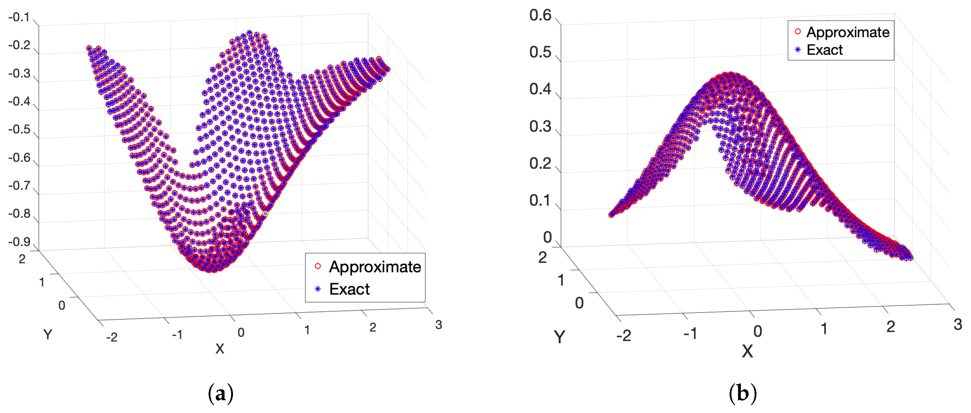
Figure 8 displays the exact and approximate values for the real and imaginary parts of the complex solutions on the amoeba-shaped domain (Figure 1a). This experiment was performed at the time with a time step of , using polynomial basis functions of the order 19. The Crank–Nicolson scheme was employed for temporal discretization, and the experiment was carried out with the numbers of interior and boundary nodes and , respectively.
Figure 8.
Example 2: (a) Real part. (b) Imaginary part.
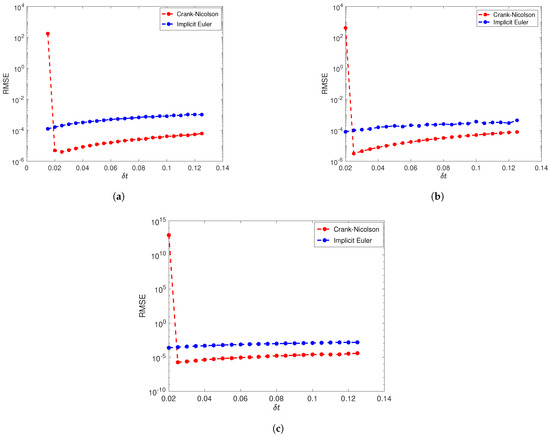
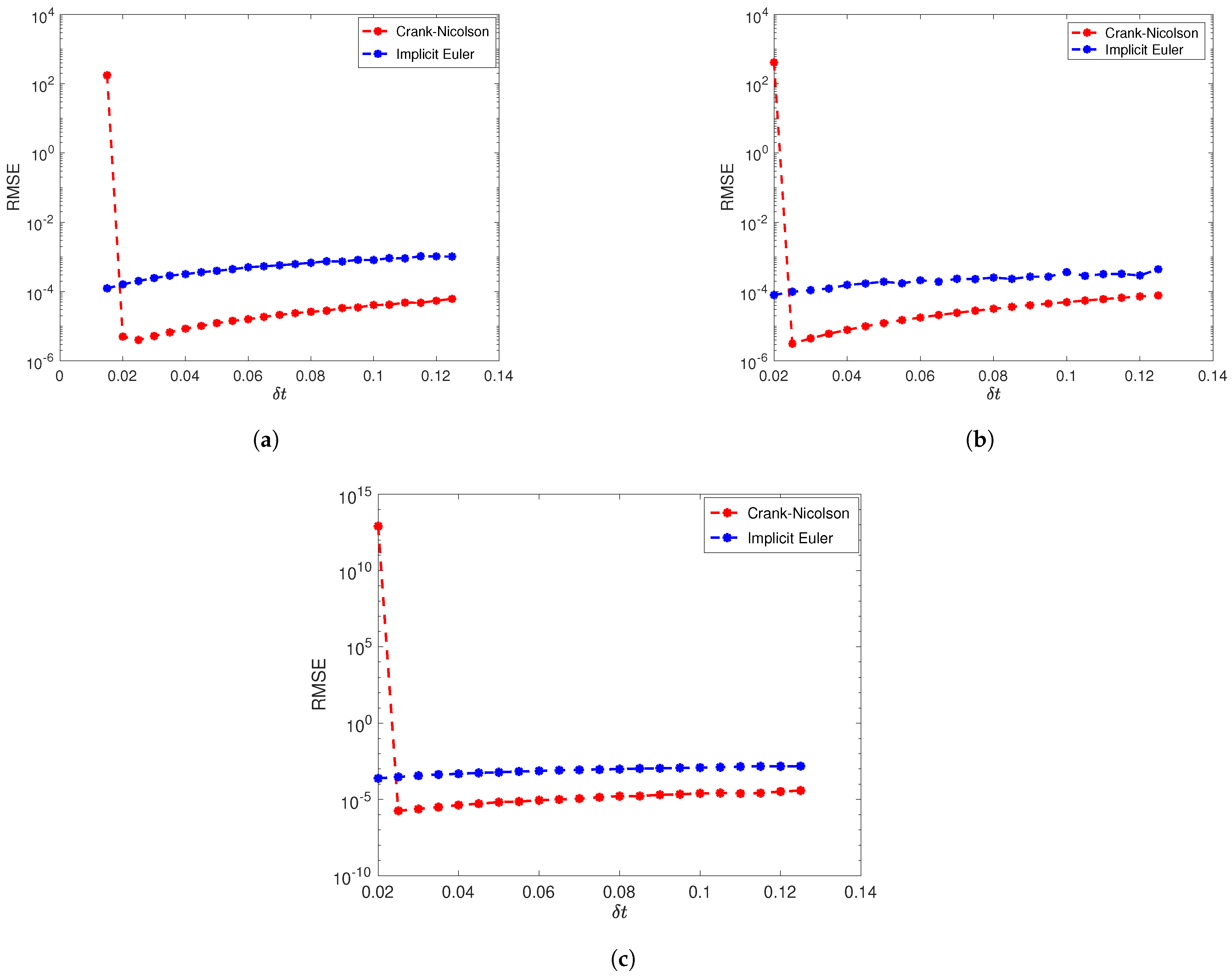
Figure 9a–c present the effect of temporal discretization at different terminal times using the Crank–Nicolson and backward Euler schemes. The problem was solved on the unit square domain with and taking polynomial basis functions of the order 13. The RMSE in these figures was computed for real parts of the solution of the given problem. We clearly notice that Crank–Nicolson scheme worked better than the backward Euler scheme with this numerical method. We also observe that the backward Euler method was suitable for smaller time steps whereas Crank–Nicolson scheme required relatively larger time steps.
Figure 9.
Example 2: Comparison of Crank–Nicolson and backward Euler methods in different time steps. (a) T = 1. (b) T = 5. (c) T = 10.
Additionally, we tested the numerical stability of our proposed method by introducing normally distributed noises at both interior and boundary nodes with varying standard deviations. A Cassini-shaped domain was considered for this experiment with interior nodes and boundary nodes. Polynomial basis functions of the order 13 were employed to perform this experiment. Table 4 demonstrates the numerical accuracy of our algorithm for real parts of the solutions using the backward Euler scheme after introducing noises. Similarly, Table 5 shows the accuracy of our algorithm for the imaginary parts of the solutions when the Crank–Nicolson scheme was used under the same conditions. From these observations, we conclude that our numerical method is highly stable for solving the time-dependent Schrödinger equation.
Table 4.
Example 2: RMSE and for real parts of solutions with different noise levels at computational nodes on Cassini-shaped domain using backward Euler scheme.
Table 5.
Example 2: RMSEs and for imaginary parts of solutions with different noise levels at computational nodes on Cassini-shaped domain using Crank–Nicolson scheme.
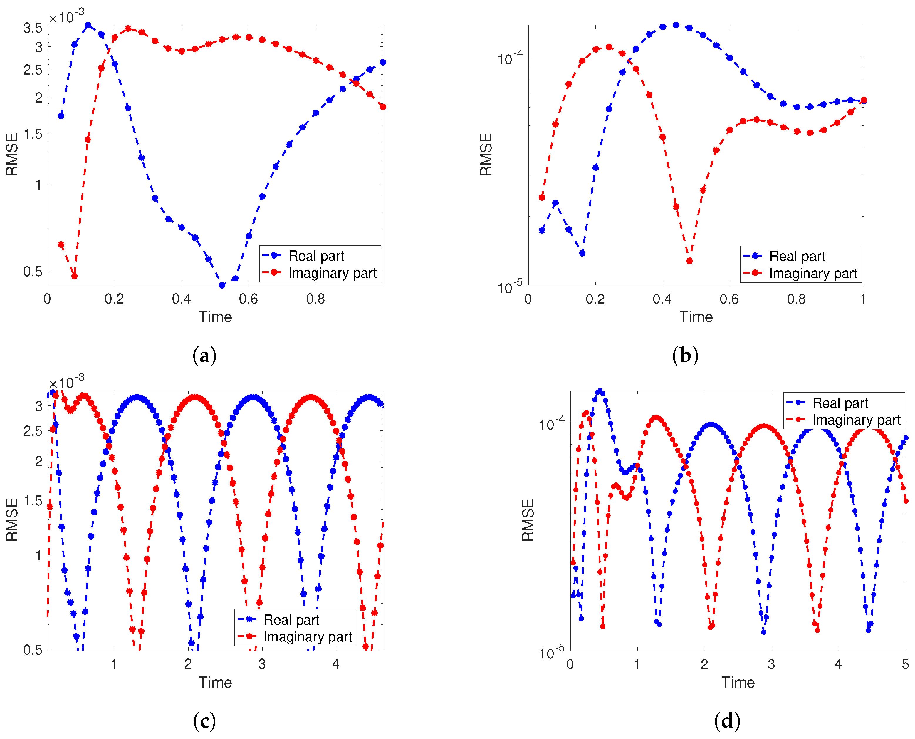
Example 3.
This experiment was performed on a unit square domain with interior nodes and boundary nodes. Polynomial basis functions of orders up to 10 was sufficient to achieve an accuracy of . The accuracy of the method using both temporal discretization techniques was reported at various terminal times for the real and imaginary parts of the solutions. The time step was set to Figure 10 clearly shows that the method produced highly accurate numerical results for both the real and imaginary parts of the solutions. Notably, the Crank–Nicolson scheme yielded slightly higher numerical accuracy than the backward Euler method, consistently with our previous examples.
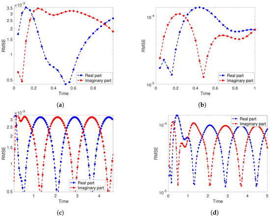
Figure 10.
Example 3: RMSE versus time for real and imaginary parts of solutions using both time discretization techniques. (a) Backward Euler. (b) Crank–Nicolson. (c) Backward Euler. (d) Crank–Nicolson.
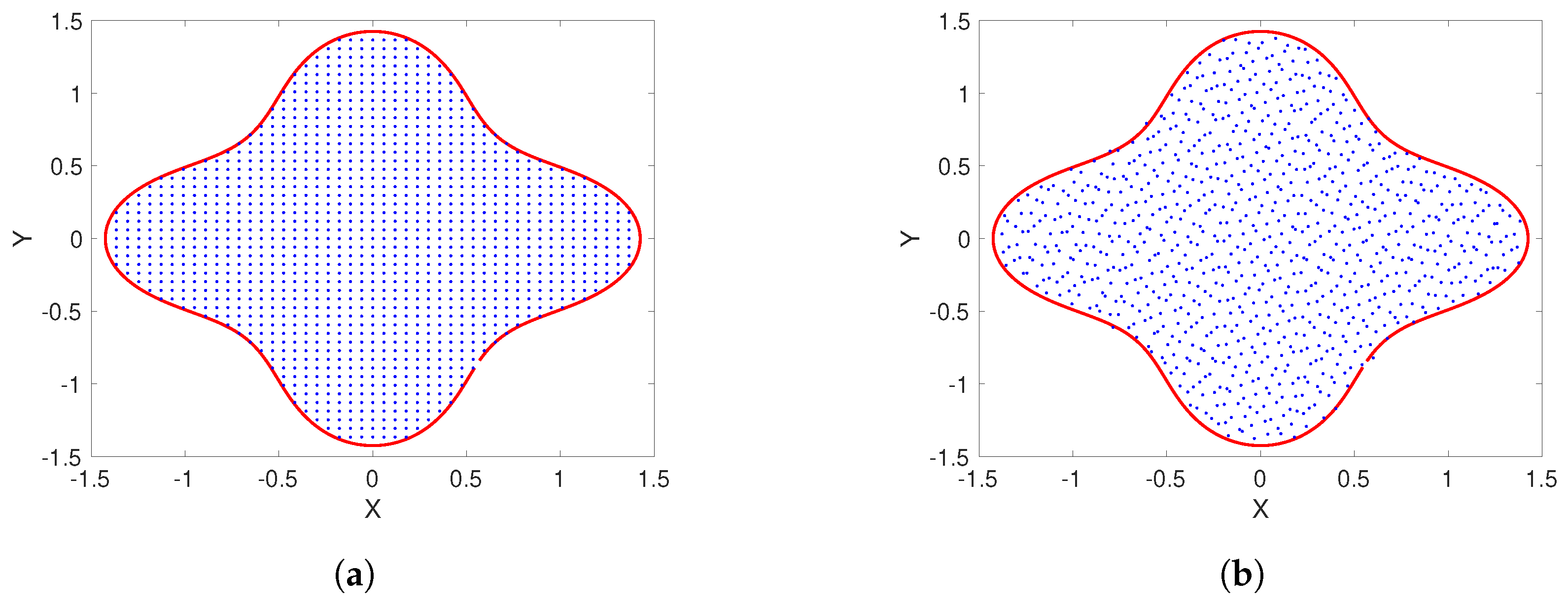
Next, we solved this problem on a Cassini-shaped domain using uniform and randomly selected (non-uniform) collocation points. The numbers of interior and boundary nodes were set to and , respectively, and the Crank–Nicolson method was used for the temporal discretization. We successfully solved the problem and the accuracy of the method was tested with various time steps using uniform and non-uniform distributions of collocation nodes. From Table 6, we clearly observe that our numerical method exhibited minimal sensitivity on the distributions of the collocation nodes in this experiment.
Table 6.
Example 3: Comparison of RMSE for uniform and non uniform distribution of collocation nodes for various time steps at terminal time .
The profiles of uniform and non-uniform collocation nodes are displayed in Figure 11.
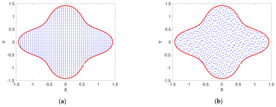
Figure 11.
Example 3: Cassini-shaped domain with uniform and non–uniform sets of nodes. (a) Uniform nodes. (b) Non–uniform nodes.
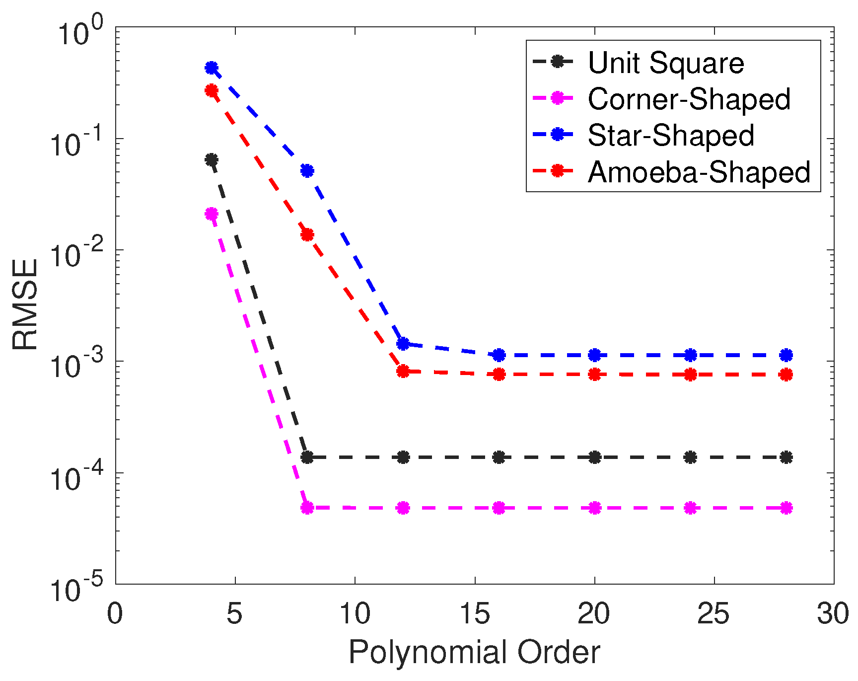
Now, we describe how we tested our numerical method on four different computational domains—a unit square, a corner-shaped domain, a star-shaped domain, and an amoeba-shaped domain—using the Crank–Nicolson method. The interior and boundary nodes for this experiment were taken to be and , respectively. Figure 12 displays the RMSE versus polynomial order for the different computational domains. From this figure, we clearly observe that the solution converged once the order of the basis functions exceeded 10 and remained stable thereafter. In most of our experiments, a polynomial basis function of the order 13 provided sufficient accuracy while solving the time-dependent Schrödinger equation.
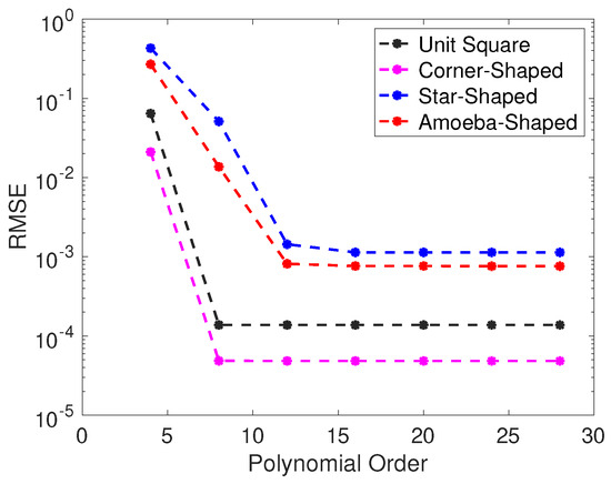
Figure 12.
Example 3: RMSE versus polynomial order for real parts of solutions using different computational domains.
Example 4.
Finally, we solved the Schrödinger Equations (1)–(4) with mixed boundary conditions. Here, the potential function for this problem was
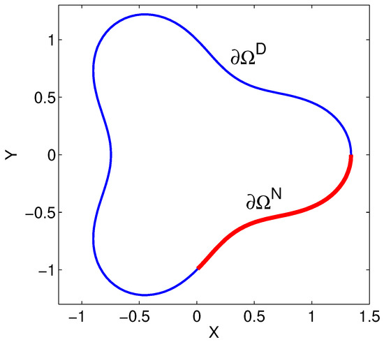
For this experiment, we chose an irregular domain (Figure 13) with the Neumann boundary condition imposed on the part of the boundary in the fourth quadrant.
Figure 13.
Computational domain with Dirichlet (blue) and Neumann (red) boundaries.
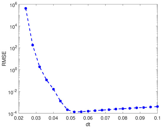
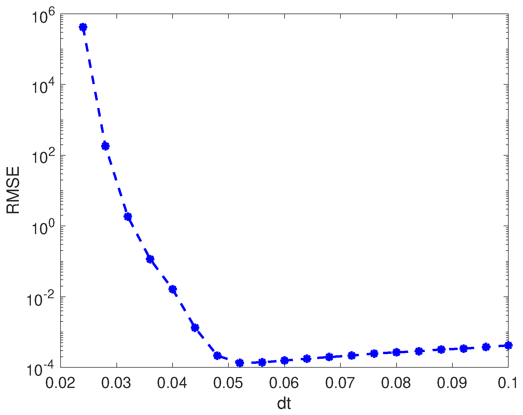
Figure 14 displays the profile of the RMSE versus the time step for the terminal time using the MPS-PBF method.
Figure 14.
Profile of RMSE vs time step for terminal time .
The interior and boundary nodes were 545 and 150, respectively. The Dirichlet boundary condition was applied on 116 nodes and the Neumann boundary condition was applied on 34 nodes. We observe that our proposed method provided the best results for a time step size of for the terminal time .
Next, Table 7 presents the numerical results for various terminal times . It is evident from the table that our proposed method performed well with both temporal discretization techniques, yielding acceptable results for the Schrödinger equation with mixed boundary conditions.
Table 7.
Example 4: Comparison of RMSEs between two temporal discretization techniques for various terminal times.
4. Conclusions and Future Work
In this paper, we employed the method of particular solutions using polynomial basis functions to solve the two-dimensional time-dependent Schrödinger equation. Unlike the traditional MPS approach which relies on radial basis functions with shape parameters, our method utilizes the polynomial basis functions in the solution process to avoid the shape parameter of the radial basis functions. For the temporal discretization, we implemented the backward Euler method and Crank–Nicolson method using various time steps and terminal times. Four numerical examples are presented to validate the effectiveness of our numerical method including one example with mixed boundary conditions. The results demonstrate that our method maintained stable and consistent numerical accuracy, even in the presence of added noise. We also compared the numerical accuracy with that of the existing MPS-RBF method, and our method was stable and clearly outperformed the accuracy of the MPS-RBF. All of these numerical examples clearly demonstrate that our numerical method is highly accurate, stable, efficient, and easy to implement. In future work, we plan to implement this robust numerical scheme to solve the non-linear time-dependent Schrödinger equation and Fisher equation.
Author Contributions
Conceptualization, T.R.D., B.K.G. and A.R.L.; Methodology, T.R.D., B.K.G. and A.R.L.; Investigation, T.R.D., B.K.G. and A.R.L.; Writing—original draft, T.R.D., B.K.G. and A.R.L.; Writing—review & editing, T.R.D., B.K.G. and A.R.L. All authors have read and agreed to the published version of the manuscript.
Funding
This research received no external funding.
Data Availability Statement
Data are contained within the article.
Conflicts of Interest
The authors declare no conflict of interest.
References
- Griffiths, D. Introduction to Quantum Mechanics, 2nd ed.; Prentice Hall: Englewood Cliff, NJ, USA, 2004. [Google Scholar]
- Arnold, A. Numerically absorbing boundary conditions for quantum evolution equations. VLSI Des. 1998, 6, 313–319. [Google Scholar] [CrossRef]
- Levy, M. Parabolic Equation Methods for Electromagnetic Wave Propagation; The Institution of Engineering and Technology: Stevenage, UK, 2000. [Google Scholar]
- Huang, W.; Xu, C.; Chu, S.T.; Chaudhuri, S.K. The finite difference vector bean propagation method. J. Light. Technol. 1992, 10, 295–304. [Google Scholar] [CrossRef]
- Kalita, J.C.; Chhabra, P.; Kumar, S. A semi-discrete higher order compact scheme for the unsteady two-dimensional Schrödinger equation. J. Comput. Appl. Math. 2006, 197, 141–149. [Google Scholar] [CrossRef]
- Subasi, M. On the finite-differences schemes for the numerical solution of two dimensional Schrödinger equation. Numer. Methods Partial Differ. Equ. 2002, 18, 752–758. [Google Scholar] [CrossRef]
- Dehghan, M. Finite difference procedures for solving a problem arising in modeling and design of certain optoelectronic devices. Math. Comput. Simul. 2006, 71, 16–30. [Google Scholar] [CrossRef]
- Feng, Y.; Zhang, X.; Chen, Y.; Wei, L. A compact finite difference scheme for solving fractional Black-Scholes option pricing model. J. Inequalities Appl. 2025, 2025, 36. [Google Scholar] [CrossRef]
- Zhang, X.; Wei, L.; Liu, J.M. Application of the LDG method using generalized alternating numerical flux to the fourth-order time-fractional sub-diffusion model. Appl. Math. Lett. 2025, 168, 109580. [Google Scholar] [CrossRef]
- Dehghan, M.; Shokri, A. A numerical method for two-dimensional Schrödinger equation using collocation and radial basis functions. Comput. Math. Appl. 2007, 54, 136–146. [Google Scholar] [CrossRef]
- Montegranario, H.; Londono, M.A.; Giraldo-Gomez, J.D.; Restrepo, R.L.; Mora-Ramos, M.E.; Duque, C.A. Solving Schrödinger equation by meshless methods. Rev. Mex. Fis. E 2016, 62, 96–107. [Google Scholar]
- Elgharbi, S.; Essaouini, M.; Abouzaid, B.; Safouhi, H. Solving the two-dimensional time-dependent Schrödinger equation using the Sinc collocation method and double exponential transformations. Appl. Numer. Math. 2025, 208, 222–231. [Google Scholar] [CrossRef]
- Dangal, T.; Chen, C.S.; Lin, J. Polynomial particular solutions for solving elliptic partial differential equations. Comput. Math. Appl. 2017, 73, 60–70. [Google Scholar]
- Liu, C.S. A multiple scale Trefftz method for an incomplete Cauchy problem of biharmonic equation. Eng. Anal. Bound. Elem 2013, 37, 17–42. [Google Scholar] [CrossRef]


Disclaimer/Publisher’s Note: The statements, opinions and data contained in all publications are solely those of the individual author(s) and contributor(s) and not of MDPI and/or the editor(s). MDPI and/or the editor(s) disclaim responsibility for any injury to people or property resulting from any ideas, methods, instructions or products referred to in the content. |
© 2025 by the authors. Licensee MDPI, Basel, Switzerland. This article is an open access article distributed under the terms and conditions of the Creative Commons Attribution (CC BY) license (https://creativecommons.org/licenses/by/4.0/).