Novel Hybrid Function Operational Matrices of Fractional Integration: An Application for Solving Multi-Order Fractional Differential Equations

Abstract

Although fractional calculus has evolved significantly since its origin in the 1695 correspondence between Leibniz and L’Hôpital, the numerical treatment of multi-order fractional differential equations remains a challenge. Existing methods are often either computationally expensive or reliant on complex operational frameworks that hinder their broader applicability. In the present study, a novel numerical algorithm is proposed based on orthogonal hybrid functions (HFs), which were constructed as linear combinations of piecewise constant sample-and-hold functions and piecewise linear triangular functions. These functions, belonging to the class of degree-1 orthogonal polynomials, were employed to obtain the numerical solution of multi-order fractional differential equations defined in the Caputo sense. A generalized one-shot operational matrix was derived to explicitly express the Riemann–Liouville fractional integral of HFs in terms of the HFs themselves. This allowed the original multi-order fractional differential equation to be transformed directly into a system of algebraic equations, thereby simplifying the solution process. The developed algorithm was then applied to a range of benchmark problems, including both linear and nonlinear multi-order FDEs with constant and variable coefficients. Numerical comparisons with well-established methods in the literature revealed that the proposed approach not only achieved higher accuracy but also significantly reduced computational effort, demonstrating its potential as a reliable and efficient numerical tool for fractional-order modeling.

1. Introduction

Since fractional calculus (FC) was first introduced during the conversation between Leibniz and L’Hôpital on 30 September 1695 [1], FC (owing to its nonlocal and memory-preserving properties) has found widespread application across numerous scientific and engineering disciplines [2]. It has been employed extensively in the mathematical modeling of diffusion phenomena, mechanical behavior of materials, signal processing, advection–dispersion processes in fractured or porous media, and image reconstruction techniques. In addition, FC plays a critical role in describing the dynamic response of viscoelastic and viscoplastic materials under external influences, pharmacokinetics, bioengineering applications, and the behavior of mechanical systems involving damping, relaxation, and reaction kinetics. It is further relevant in modeling ultraslow diffusion and anomalous transport and in establishing connections with the theory of random walks, finance, control theory, and even cognitive processes in psychology. Beyond its interdisciplinary applications, fractional calculus possesses profound significance within mathematics itself. One of the key advantages of FC lies in its generality—encompassing the classical integer-order calculus as a particular case—thus offering a more flexible and encompassing framework for differential modeling. This generalization enables the capture of memory and hereditary characteristics inherent in many natural and engineered systems, which traditional integer-order calculus fails to describe adequately. The ability of fractional calculus to model systems with memory makes it a powerful and indispensable tool for uncovering complex dynamic behavior embedded in natural phenomena.

Since the inception of FC, many methods have been developed to solve differential equations that involve derivatives or integrals of non-integer order. Initially, analytical techniques such as the Fourier transform [3,4], modal synthesis and eigenvector expansion [5], Laplace transform, fractional Green’s function, Mellin transform, and power series method [6] were used to find exact solutions for linear fractional-order differential equations. However, it became clear that these methods often fail when dealing with nonlinear or more complex fractional differential equations. This limitation led to the development of numerical methods such as Podlubny’s numerical method [6], the Predictor-Evaluate–Corrector-Evaluate method [7], and the generalized Euler’s method [8], as well as semi-analytical methods like the Adomian decomposition method [9], the variational iteration method [10], the homotopy perturbation method [11], the fractional differential transform method [12], the homotopy analysis method [13], and the new iterative method [14], all of which aim to provide accurate and stable numerical solutions.

In recent years, there has been growing interest in using orthogonal functions or wavelets to develop new numerical techniques. These include block pulse functions, hat functions, and Chebyshev, Muntz, Laguerre, Jacobi, Legendre, and Bernstein polynomials [15,16,17,18,19,20,21,22]. Khader (2013) used generalized Laguerre polynomials in a spectral collocation method to solve the fractional Klein–Gordon equation, converting the original problem into a system of ordinary differential equations [23]. Li (2014) proposed a method using cubic B-spline functions to reduce fractional differential equations into algebraic equations, improving both accuracy and memory efficiency [24]. Muthukumar and Priya (2017) applied shifted Jacobi polynomials to solve fractional delay differential equations, using operational matrices to simplify the problem while preserving memory effects [25]. Xu and Xu (2018) designed a Legendre wavelet-based method that derives an explicit formula for fractional integrals, enabling accurate and efficient computation even with multi-point boundary conditions [26]. Further advancements were made by Talib et al. (2019), who used shifted Legendre polynomials to handle coupled systems of fractional differential equations with mixed derivatives [27]. Wang et al. (2019) applied Bernoulli wavelets to transform systems of fractional equations into algebraic systems [28]. Mall and Chakraverty (2020) introduced a Chebyshev neural network to handle nonlinear Lane–Emden equations by converting them into algebraic form [29]. Hosseininia et al. (2021) combined Bernoulli polynomials and radial basis functions to solve variable-order reaction–advection–diffusion equations efficiently [30]. Ahmed (2023) proposed a spectral collocation technique using shifted Jacobi polynomials and constructed operational matrices for both regular and variable-order derivatives [31]. Matoog et al. (2024) applied Hermite polynomials and the Ramadan group transform to reduce fractional integro-differential equations to algebraic systems [32]. Azarnavid et al., (2024) used integrated Bernoulli polynomials and collocation at shifted Chebyshev points to build an iterative solver for nonlinear multi-order fractional equations [33]. Chaudhary et al. (2024) introduced Vieta–Lucas polynomials with the Tau method to solve systems of fractional differential equations by reducing them into algebraic systems [34]. Manohara and Kumbinarasaiah (2025) used Genocchi wavelets to solve a fractional diabetes model by constructing an operational matrix that simplifies computation while ensuring high accuracy [35]. All these numerical algorithms share a key strength: they transform fractional differential equations into systems of algebraic equations. Once this transformation is accomplished, solving the problem becomes much easier and faster. That is why building numerical methods using orthogonal functions is so beneficial.

A new type of orthogonal function, called hybrid functions (HFs), was introduced in [36]. These combine piecewise constant and piecewise linear functions and are classified as degree-1 orthogonal polynomials. HFs were initially used to solve integer-order systems with or without delays [37], and they have great potential in solving fractional-order problems as well. Although few studies have explored this yet, as shown in the following sections, these hybrid functions could play a powerful role in the future of fractional calculus. The present work brings forward one of the important applications of the new orthogonal hybrid functions for solving multi-order fractional differential equation (FDE) of the form:

$$D^{\alpha }y\left(t\right)={\displaystyle \sum _{k=1}^r{b}_k\left(t\right)D^{{\beta }_k}y\left(t\right)}+b_0\left(t\right){\left(y\left(t\right)\right)}^p+g\left(t\right), t\in \left[0,1\right], \alpha \in \left(n-1,n\right], n\in Z^{+}$$

(1)

Here, $\alpha >{\beta }_1>{\beta }_2>\cdots \cdots {\beta }_r$, $b_k\left(t\right)$, $b_0\left(t\right)$, and $g\left(t\right)$ are given functions of the independent variable $t$, $p$ is an arbitrary number, $y\left(t\right)$ is the unknown function, and $D^{\alpha }y\left(t\right)$ is the Caputo fractional order derivative defined as [38]:

$$D^{\alpha }f\left(t\right)=J^{n-\alpha }{D}^{n}f\left(t\right)={\displaystyle \frac{1}{\mathrm{\Gamma }\left(m-\alpha \right)}}{\displaystyle \underset{0}{\overset{t}{\int }}{\left(t-\tau \right)}^{n-\alpha -1}{f}^{\left(n\right)}\left(\tau \right)d\tau },$$

(2)

where $J^{\alpha }f\left(t\right)$ is Riemann–Liouville fractional order integral [1], $J^{\alpha }f\left(t\right)={\displaystyle \frac{1}{\mathrm{\Gamma }\left(\alpha \right)}}{\displaystyle \underset{0}{\overset{t}{\int }}{\left(t-\tau \right)}^{\alpha -1}}f\left(\tau \right)d\tau$.

To accomplish the goal of numerically solving the multi-order fractional differential equation in Equation (1) using HFs, we first derive a formula, by means of generalized one-shot operational matrices, explicitly expressing the fractional order integral of HFs in terms of the HFs themselves, and in the second step we make use of the derived generalized one-shot operational matrices to transform Equation (1) into a system of algebraic equations whose solution is the approximate solution of Equation (1).

Motivation and Contributions

Despite significant advancements in numerical methods for solving fractional differential equations (FDEs), several limitations continue to persist in the existing literature. While many of the reported methods rely on orthogonal functions such as Chebyshev, Legendre, Jacobi, Laguerre, and Bernstein polynomials, etc., the derivation of an operational matrix to approximate either a fractional order integral or a fractional order derivative requires complex calculations and is computationally expensive. In addition, these methods suffer from accuracy-related issues when applied to highly nonlinear fractional order differential equations. To address these challenges, the present work introduces a new numerical strategy based on HFs, which provide a flexible and computationally light alternative to classical orthogonal polynomials. Although HFs were originally developed for integer-order systems, their potential in the context of fractional calculus has remained largely unexplored.

The key contributions of the present work are as follows:

• This work introduces a novel application of orthogonal HFs for solving multi-order FDEs formulated in the Caputo fractional derivative sense.
• A generalized one-shot operational matrix was derived to approximate the fractional-order integral of HFs, expressing the integral explicitly in terms of HFs themselves.
• The derived operational matrix was applied to transform the original multi-order FDEs into a system of algebraic equations, significantly simplifying the computational process. The resulting algebraic equations were solved using a nonlinear algebraic solver.
• The developed numerical algorithm was applied to a set of linear and nonlinear multi-order FDEs to demonstrate the applicability of the proposed algorithm to a wide variety of multi-order FDEs.
• A comparative study was conducted to highlight the superior performance of the proposed algorithm over the existing methods.

The remaining paper is structured as follows. Section 2 introduces new orthogonal hybrid functions. The generalized one-shot operational matrices are derived in Section 3. Based on the results of Section 3, a new numerical algorithm is proposed in Section 4. In Section 5, we test our numerical algorithm by applying it to a set of test problems consisting of linear and nonlinear multi-order fractional differential equations. Section 6 presents the significant inferences drawn from the present work.

2. Orthogonal Hybrid Functions

Let us consider the time function, $f\left(t\right)$, of the Lebesgue measure, which is defined on the interval $\left[0,T\right)$. We split the interval into an $m$ number of subintervals using the constant step size $h$.

$$\left[0,h\right), \left[h,2h\right), \left[2h,3h\right), \dots \dots \dots , \left[jh,\left(j+1\right)h\right), \dots \dots \dots , \left[\left(m-1\right)h,mh\right)$$

(3)

We now state an $m$-term hybrid function vector, $H_{\left(m\right)}\left(t\right)$, each of which represents the original function, f(t), in the respective subinterval.

$$H_{\left(m\right)}\left(t\right)={\left[H_0\left(t\right) H_1\left(t\right) H_2\left(t\right) \cdots H_i\left(t\right) \cdots \cdots H_{m-1}\left(t\right)\right]}^{Tp}$$

(4)

where ‘$Tp$’ indicates transpose.

The $i^{\mathit{th}}$ hybrid function, $H_i\left(t\right)$, is defined as

$$H_i\left(t\right)=c_i{S}_i\left(t\right)+d_i{T}_i\left(t\right), i\in \left[0,m-1\right],$$

(5)

where $c_i$ and $d_i$ are arbitrary constants and $S_i\left(t\right)$ is the $i^{\mathit{th}}$ sample-and-hold function (SHF) described as

$$S_i\left(t\right)=\left\{\begin{array}{cc}1,\hfill & i\mathrm{f} t\in \left[ih,\left(i+1\right)h\right),\\ 0,\hfill & \mathrm{otherwise},\end{array}\right.\begin{array}{c}\hspace{1em}\\ i\in \left[0,m-1\right],\end{array}$$

(6)

$T_i\left(t\right)$ is the $i^{\mathit{th}}$ right-handed triangular function (TF)

$$T_i\left(t\right)=\left\{\begin{array}{cc}{\displaystyle \frac{t-ih}{h}},& i\mathrm{f} t\in \left[ih,\left(i+1\right)h\right),\\ 0,& \mathrm{otherwise},\end{array}\right.\begin{array}{c}\hspace{1em}\\ i\in \left[0,m-1\right].\end{array}$$

(7)

Using Equations (5)–(7), the actual function, f(t), can be approximated piecewise, as shown below:

$$f\left(t\right)\approx {\displaystyle \sum _{i=0}^{m-1}{H}_i\left(t\right)=}{\displaystyle \sum _{i=0}^{m-1}\left(c_i{S}_i\left(t\right)+d_i{T}_i\left(t\right)\right)}=C_S^T{S}_{\left(m\right)}\left(t\right)+C_T^T{T}_{\left(m\right)}\left(t\right)$$

(8)

where $C_S^T=\left[c_0 c_1 \cdots \cdots c_{m-1}\right]$, $C_T^T=\left[d_0 d_1 \cdots \cdots d_{m-1}\right]$, $d_i=c_{i+1}-c_i$, $c_i=f\left(ih\right)$, $S_{\left(m\right)}\left(t\right)={\left[S_o\left(t\right) S_1\left(t\right) \cdots \cdots S_{m-1}\left(t\right)\right]}^{Tp}$, and $T_{\left(m\right)}\left(t\right)={\left[T_0\left(t\right) T_1\left(t\right) \cdots \cdots T_{m-1}\left(t\right)\right]}^{Tp}$.

The first order integral of $S_{\left(m\right)}\left(t\right)$ is estimated in the orthogonal HF domain as follows:

$${\displaystyle \underset{0}{\overset{t}{\int }}{S}_{\left(m\right)}\left(\tau \right)d\tau }=P_{1ss\left(m\right)}{S}_{\left(m\right)}\left(t\right)+P_{1st\left(m\right)}{T}_{\left(m\right)}\left(t\right)$$

(9)

where $P_{1ss\left(m\right)}=h{\left[\left[\left.\left.0 1 1 \cdots \cdots 1\right]\right]\right.\right.}_{m\times m}$, $P_{1st\left(m\right)}=h{\left[\left[\left.\left.1 0 0 \cdots \cdots 0\right]\right]\right.\right.}_{m\times m}$, and $\left[\left[\left.\left.\begin{array}{cccc}a& b& c& d\end{array}\right]\right]\right.\right.=\left[\begin{array}{cccc}a& b& c& d\\ 0& a& b& c\\ 0& 0& a& b\\ 0& 0& 0& a\end{array}\right]$.

In the same way, the right-handed triangular function vector, $T_{\left(m\right)}\left(t\right)$, is integrated once, and the result is expanded into orthogonal HF series

$${\displaystyle \underset{0}{\overset{t}{\int }}{T}_{\left(m\right)}\left(\tau \right)d\tau }=P_{1ts\left(m\right)}{S}_{\left(m\right)}\left(t\right)+P_{1tt\left(m\right)}{T}_{\left(m\right)}\left(t\right)$$

(10)

where $P_{1ts\left(m\right)}={\displaystyle \frac{h}{2}}{\left[\left[\left.\left.0 1 1 \cdots \cdots 1\right]\right]\right.\right.}_{m\times m}$ and $P_{1tt\left(m\right)}={\displaystyle \frac{h}{2}}{\left[\left[\left.\left.1 0 0 \cdots \cdots 0\right]\right]\right.\right.}_{m\times m}$.

Employing Equations (9) and (10),

$$\begin{array}{lll}{\displaystyle \underset{0}{\overset{t}{\int }}f\left(\tau \right)d\tau }& \approx & {\displaystyle \underset{0}{\overset{t}{\int }}\left(C_S^T{S}_{\left(m\right)}\left(\tau \right)+C_T^T{T}_{\left(m\right)}\left(\tau \right)\right)d\tau }=C_S^T{\displaystyle \underset{0}{\overset{t}{\int }}{S}_{\left(m\right)}\left(\tau \right)d\tau }+C_T^T{\displaystyle \underset{0}{\overset{t}{\int }}{T}_{\left(m\right)}\left(\tau \right)d\tau ,}\\ \hspace{1em}& =& C_S^T\left(P_{1ss\left(m\right)}{S}_{\left(m\right)}\left(t\right)+P_{1st\left(m\right)}{T}_{\left(m\right)}\left(t\right)\right)+C_T^T\left(P_{1ts\left(m\right)}{S}_{\left(m\right)}\left(t\right)+P_{1tt\left(m\right)}{T}_{\left(m\right)}\left(t\right)\right),\\ \hspace{1em}& =& \left(C_S^T{P}_{1ss\left(m\right)}+C_T^T{P}_{1ts\left(m\right)}\right)S_{\left(m\right)}\left(t\right)+\left(C_S^T{P}_{1st\left(m\right)}+C_T^T{P}_{1tt\left(m\right)}\right)T_{\left(m\right)}\left(t\right),\end{array}$$

(11)

where $P_{1ss\left(m\right)}$, $P_{1st\left(m\right)}$, $P_{1ts\left(m\right)}$, and $P_{1tt\left(m\right)}$ are called the complementary one-shot operational matrices of first order integration and act as a first-order integrator in the orthogonal HF domain. The orthogonal properties and a few operational properties of HFs are listed in Appendix A.1.

3. Generalized One-Shot Operational Matrices for Fractional Integration

The main objective of this section is to derive an approximation using orthogonal HFs for the Riemann–Liouville fractional integral of order $\alpha$ of $f\left(t\right)$.

Theorem 1.

Let $\alpha \in \left(n-1,n\right]$, $n$ be an integer, and $t\in \left[0,T\right]$.The fractional integral of order $\alpha$ of the SHF vector, $S_{\left(m\right)}\left(t\right)$, is obtained in the orthogonal HF domain as

$$J^{\alpha }{S}_{\left(m\right)}\left(t\right)={\displaystyle \frac{1}{\mathrm{\Gamma }\left(\alpha \right)}}{\displaystyle \underset{0}{\overset{t}{\int }}{\left(t-\tau \right)}^{\alpha -1}{S}_{\left(m\right)}\left(\tau \right)d\tau }=P_{\alpha ss\left(m\right)}{S}_{\left(m\right)}\left(t\right)+P_{\alpha st\left(m\right)}{T}_{\left(m\right)}\left(t\right)$$

(12)

where $P_{\alpha ss\left(m\right)}={\displaystyle \frac{h^{\alpha }}{\mathrm{\Gamma }\left(\alpha +1\right)}}\left[\left[\left.\left.0 {\varsigma }_1 {\varsigma }_2 {\varsigma }_3 \cdots {\varsigma }_{m-1}\right]\right]\right.\right.$, ${\varsigma }_k=\left(k^{\alpha }-{\left(k-1\right)}^{\alpha }\right)$, $k\in \left[1,m-1\right]$, $P_{\alpha st\left(m\right)}={\displaystyle \frac{h^{\alpha }}{\mathrm{\Gamma }\left(\alpha +1\right)}}\left[\left[\left.\left.1 {\xi }_1 {\xi }_2 {\xi }_3 \cdots {\xi }_{m-1}\right]\right]\right.\right.$, ${\xi }_k={\left(k+1\right)}^{\alpha }-2k^{\alpha }+{\left(k-1\right)}^{\alpha }$, and $k\in \left[1,m-1\right]$.

Proof. 

The proof is given in Appendix A.2. □

Remark. 

If $\alpha =1$, then ${\varsigma }_k=1$, $\forall k\in \left[1,m-1\right]$, ${\xi }_k=0$, and $\forall k\in \left[1,m-1\right]$; thus, Equation (12) produces the same result as Equation (9).

Theorem 2.

The fractional integral of order $\alpha$($\alpha \in \left(n-1,n\right],n\in Z^{+}$) of the right-handed triangular function vector, $T_{\left(m\right)}\left(t\right)$, is expressed by means of orthogonal HFs:

$$J^{\alpha }{T}_{\left(m\right)}\left(t\right)={\displaystyle \frac{1}{\mathrm{\Gamma }\left(\alpha \right)}}{\displaystyle \underset{0}{\overset{t}{\int }}{\left(t-\tau \right)}^{\alpha -1}{T}_{\left(m\right)}\left(\tau \right)d\tau }=P_{\alpha ts\left(m\right)}{S}_{\left(m\right)}\left(t\right)+P_{\alpha tt\left(m\right)}{T}_{\left(m\right)}\left(t\right)$$

(13)

$$P_{\alpha ts\left(m\right)}={\displaystyle \frac{h^{\alpha }}{\mathrm{\Gamma }\left(\alpha +2\right)}}\left[\left[\left.\left.0 {\varphi }_1 {\varphi }_2 {\varphi }_3 \cdots {\varphi }_{m-1}\right]\right]\right.\right., P_{\alpha tt\left(m\right)}={\displaystyle \frac{h^{\alpha }}{\mathrm{\Gamma }\left(\alpha +2\right)}}\left[\left[\left.\left.1 {\psi }_1 {\psi }_2 {\psi }_3 \cdots {\psi }_{m-1}\right]\right]\right.\right.$$

$${\varphi }_k=k^{\alpha +1}-{\left(k-1\right)}^{\alpha }\left(k+\alpha \right), {\psi }_k={\left(k+1\right)}^{\alpha +1}-\left(k+1+\alpha \right)k^{\alpha }-k^{\alpha +1}+\left(k+\alpha \right){\left(k-1\right)}^{\alpha }, \mathrm{and} k\in \left[1,m-1\right].$$

Proof. 

Appendix A.3. presents the proof of Theorem 2. □

Remark. 

Since ${\varphi }_k=1$ and ${\psi }_k=0$ for $\alpha =1$ and $k\in \left[1,m-1\right]$ , the result of Equation (10) can be recovered from Equation (13).

Theorem 3.

The HF approximation for the Riemann–Liouville fractional order integral of the function $f\left(t\right)$ is

$${\displaystyle \frac{1}{\mathrm{\Gamma }\left(\alpha \right)}}{\displaystyle \underset{0}{\overset{t}{\int }}{\left(t-\tau \right)}^{\alpha -1}f\left(\tau \right)d\tau \approx \left(C_S^T{P}_{\alpha ss\left(m\right)}+C_T^T{P}_{\alpha ts\left(m\right)}\right)}{S}_{\left(m\right)}\left(t\right)+\left(C_S^T{P}_{\alpha st\left(m\right)}+C_T^T{P}_{\alpha tt\left(m\right)}\right)T_{\left(m\right)}\left(t\right).$$

(14)

Proof. 

Using Equation (8) in the definition of the Riemann–Liouville fractional order integral of $f\left(t\right)$ is

$$\begin{array}{l}{J}^{\alpha }f\left(t\right)={\displaystyle \frac{1}{\mathrm{\Gamma }\left(\alpha \right)}}{\displaystyle \underset{0}{\overset{t}{\int }}{\left(t-\tau \right)}^{\alpha -1}f\left(\tau \right)d\tau }\approx {\displaystyle \frac{1}{\mathrm{\Gamma }\left(\alpha \right)}}{\displaystyle \underset{0}{\overset{t}{\int }}{\left(t-\tau \right)}^{\alpha -1}\left(C_S^T{S}_{\left(m\right)}\left(\tau \right)+C_T^T{T}_{\left(m\right)}\left(\tau \right)\right)d\tau ,}\\ \hspace{1em}\hspace{1em}\hspace{1em}\hspace{1em}\hspace{1em}\hspace{1em}\hspace{1em}\hspace{1em}\hspace{1em}=C_S^T\left({\displaystyle \frac{1}{\mathrm{\Gamma }\left(\alpha \right)}}{\displaystyle \underset{0}{\overset{t}{\int }}{\left(t-\tau \right)}^{\alpha -1}{S}_{\left(m\right)}\left(\tau \right)d\tau }\right)+C_T^T\left({\displaystyle \frac{1}{\mathrm{\Gamma }\left(\alpha \right)}}{\displaystyle \underset{0}{\overset{t}{\int }}{\left(t-\tau \right)}^{\alpha -1}{T}_{\left(m\right)}\left(\tau \right)d\tau }\right).\end{array}$$

(15)

From Theorems 1 and 2, we can obtain the expression in Equation (14). This completes the proof. □

Remark. 

The generalized HF approximation in Equation (14) yields the HF estimate for the first-order integration of  $f\left(t\right)$  in special case $\alpha =1$.

• Example 3.1

We now test the viability of the generalized one-shot operational matrices–based HF approximation ($J_{HF}^{\alpha }f\left(t\right)$) for the Riemann–Liouville fractional order integral of $f\left(t\right)$. Let us consider a time function $f\left(t\right)=t$, $t\in \left[0,1\right]$ and a step size of 0.125.

The exact fractional order integral of $f\left(t\right)$ is

$$J^{\alpha }f\left(t\right)={\displaystyle \frac{\mathrm{\Gamma }\left(1+1\right)t^{1+\alpha }}{\mathrm{\Gamma }\left(2+\alpha \right)}}, \alpha \in \left(0,5\right].$$

(16)

Table 1. Performance of HF approximation.

$\mathit{\alpha }$	${‖{\mathit{J}}^{\mathit{\alpha }}\mathit{f}\left(\mathit{t}\right)-{\mathit{J}}_{\mathit{H}\mathit{F}}^{\mathit{\alpha }}\mathit{f}\left(\mathit{t}\right)‖}_{\mathit{\infty }}$	CPU Time (s)
0.5	1.11022302462516 × 10−16	0.021720
1	0	0.020514
1.5	5.551115123125783 × 10−17	0.022866
2	2.775557561562891 × 10−17	0.021033
2.5	1.387778780781446 × 10−17	0.023839
3	6.938893903907228 × 10−18	0.021494
3.5	8.673617379884035 × 10−19	0.021404
4	0	0.022049
4.5	1.084202172485504 × 10−19	0.021662
5	2.168404344971009 × 10−19	0.021855

presents the $\infty$-norm of the error between the exact fractional integral and its approximation in the orthogonal HF domain for various of $\alpha$. It is noticed from Table 1 that the formula in Equation (14) approximates both the integer order and the non-integer order integral of $f\left(t\right)$ with high accuracy. Even though the HF estimate for $J^{\alpha }f\left(t\right)$ may seem complex, it requires much less CPU usage. The approach of estimating the Riemann–Liouville fractional integral using the generalized one-shot operational matrices is reliable, exact, and computationally effective.

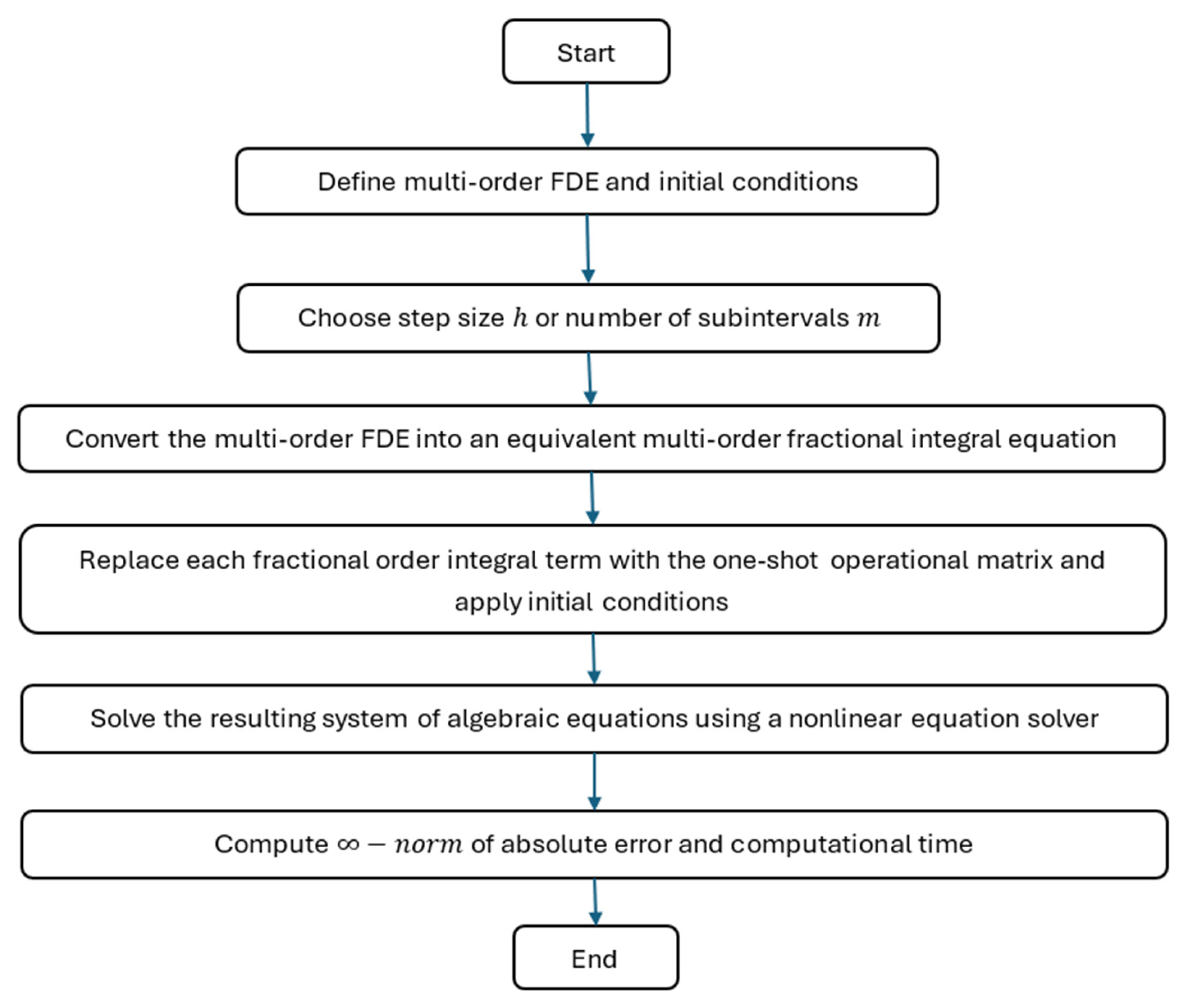
4. Algorithm for Solving Multi-Order FDEs (HFM)

We now explain the procedure of finding the approximate solution of the multi-order FDE by the application of the generalized one-shot operational matrices derived in the previous section.

Let us recall the general form of the multi-order FDE:

$$D^{\alpha }y\left(t\right)={\displaystyle \sum _{k=1}^r{b}_k\left(t\right)D^{{\beta }_k}y\left(t\right)}+b_0\left(t\right){\left(y\left(t\right)\right)}^p+g\left(t\right), t\in \left[0,1\right], \alpha \in \left(n-1,n\right], n\in Z^{+}$$

(17)

For the sake of simplicity, we consider the homogeneous initial conditions $y^{\left(s\right)}\left(0\right)=0$ and $s=0,1,2,\dots \dots ,n-1$.

Let

$$D^{\alpha }y\left(t\right)\approx C_S^T{S}_{\left(m\right)}\left(t\right)+C_T^T{T}_{\left(m\right)}\left(t\right)$$

(18)

$$\begin{array}{l}{D}^{{\beta }_k}y\left(t\right)\approx J^{\alpha -{\beta }_k}\left(C_S^T{S}_{\left(m\right)}\left(t\right)+C_T^T{T}_{\left(m\right)}\left(t\right)\right)\\ \hspace{1em}\hspace{1em}=C_S^T\left(P_{\left(\alpha -{\beta }_k\right)ss\left(m\right)}{S}_{\left(m\right)}\left(t\right)+P_{\left(\alpha -{\beta }_k\right)st\left(m\right)}{T}_{\left(m\right)}\left(t\right)\right)+C_T^T\left(P_{\left(\alpha -{\beta }_k\right)ts\left(m\right)}{S}_{\left(m\right)}\left(t\right)+P_{\left(\alpha -{\beta }_k\right)tt\left(m\right)}{T}_{\left(m\right)}\left(t\right)\right)\\ \hspace{1em}\hspace{1em}=\left(C_S^T{P}_{\left(\alpha -{\beta }_k\right)ss\left(m\right)}+C_T^T{P}_{\left(\alpha -{\beta }_k\right)ts\left(m\right)}\right)S_{\left(m\right)}\left(t\right)+\left(C_S^T{P}_{\left(\alpha -{\beta }_k\right)st\left(m\right)}+C_T^T{P}_{\left(\alpha -{\beta }_k\right)tt\left(m\right)}\right)T_{\left(m\right)}\left(t\right)\end{array}$$

(19)

$${\left(y\left(t\right)\right)}^p\approx {\tilde{C}}_S^T{S}_{\left(m\right)}\left(t\right)+{\tilde{C}}_T^T{T}_{\left(m\right)}\left(t\right) (\mathrm{using} (\mathrm{A6}))$$

(20)

$$g\left(t\right)\approx C_{S0}^T{S}_{\left(m\right)}\left(t\right)+C_{T0}^T{T}_{\left(m\right)}\left(t\right)$$

(21)

$$\begin{array}{l}y\left(t\right)\approx J^{\alpha }\left(C_S^T{S}_{\left(m\right)}\left(t\right)+C_T^T{T}_{\left(m\right)}\left(t\right)\right)\\ \hspace{1em}\hspace{1em}=\left(C_S^T{P}_{\alpha ss\left(m\right)}+C_T^T{P}_{\alpha ts\left(m\right)}\right)S_{\left(m\right)}\left(t\right)+\left(C_S^T{P}_{\alpha st\left(m\right)}+C_T^T{P}_{\alpha tt\left(m\right)}\right)T_{\left(m\right)}\left(t\right)\end{array}$$

(22)

Equation (17) becomes

$$\begin{array}{l}{C}_S^T{S}_{\left(m\right)}\left(t\right)+C_T^T{T}_{\left(m\right)}\left(t\right)={\displaystyle \sum _{k=1}^r{b}_k\left(t\right)\left(C_S^T{P}_{\left(\alpha -{\beta }_k\right)ss\left(m\right)}+C_T^T{P}_{\left(\alpha -{\beta }_k\right)ts\left(m\right)}\right)S_{\left(m\right)}\left(t\right)}+C_{S0}^T{S}_{\left(m\right)}\left(t\right)+C_{T0}^T{T}_{\left(m\right)}\left(t\right)+\\ \hspace{1em}\hspace{1em}\hspace{1em}\hspace{1em}\hspace{1em}\hspace{1em}\hspace{1em}\hspace{1em}{\displaystyle \sum _{k=1}^r{b}_k\left(t\right)\left(C_S^T{P}_{\left(\alpha -{\beta }_k\right)st\left(m\right)}+C_T^T{P}_{\left(\alpha -{\beta }_k\right)tt\left(m\right)}\right)T_{\left(m\right)}\left(t\right)}+b_0\left(t\right)\left({\tilde{C}}_S^T{S}_{\left(m\right)}\left(t\right)+{\tilde{C}}_T^T{T}_{\left(m\right)}\left(t\right)\right)\end{array}$$

(23)

Estimating the variable coefficients $b_k\left(t\right)$ and $b_0\left(t\right)$ in the HF domain,

$$b_k(t)\approx C_{S1}^T{S}_{\left(m\right)}\left(t\right)+C_{T1}^T{T}_{\left(m\right)}\left(t\right), b_0\left(t\right)\approx C_{S2}^T{S}_{\left(m\right)}\left(t\right)+C_{T2}^T{T}_{\left(m\right)}\left(t\right)$$

(24)

From Equations (23) and (24),

$$\begin{array}{l}{C}_S^T{S}_{\left(m\right)}\left(t\right)+C_T^T{T}_{\left(m\right)}\left(t\right)={\displaystyle \sum _{k=1}^r\left(C_{S1}^T{S}_{\left(m\right)}\left(t\right)+C_{T1}^T{T}_{\left(m\right)}\left(t\right)\right)\left(C_S^T{P}_{\left(\alpha -{\beta }_k\right)ss\left(m\right)}+C_T^T{P}_{\left(\alpha -{\beta }_k\right)ts\left(m\right)}\right)S_{\left(m\right)}\left(t\right)}+\\ C_{S0}^T{S}_{\left(m\right)}\left(t\right)+C_{T0}^T{T}_{\left(m\right)}\left(t\right)+{\displaystyle \sum _{k=1}^r\left(C_{S1}^T{S}_{\left(m\right)}\left(t\right)+C_{T1}^T{T}_{\left(m\right)}\left(t\right)\right)\left(C_S^T{P}_{\left(\alpha -{\beta }_k\right)st\left(m\right)}+C_T^T{P}_{\left(\alpha -{\beta }_k\right)tt\left(m\right)}\right)T_{\left(m\right)}\left(t\right)}+\\ \left(C_{S2}^T{S}_{\left(m\right)}\left(t\right)+C_{T2}^T{T}_{\left(m\right)}\left(t\right)\right)\left({\tilde{C}}_S^T{S}_{\left(m\right)}\left(t\right)+{\tilde{C}}_T^T{T}_{\left(m\right)}\left(t\right)\right)\end{array}$$

(25)

Employing Equation (A5),

$$C_S^T{S}_{\left(m\right)}\left(t\right)+C_T^T{T}_{\left(m\right)}\left(t\right)={\displaystyle \sum _{k=1}^r\left(C_1{S}_{\left(m\right)}\left(t\right)+\left(C_2+C3\right)T_{\left(m\right)}\left(t\right)\right)}+\left(C_{S0}^T+C_4\right)S_{\left(m\right)}\left(t\right)+\left(C_{T0}^T+C_5\right)T_{\left(m\right)}\left(t\right)$$

(26)

where $C_1=C_{S1·}^T*\left(C_S^T{P}_{\left(\alpha -{\beta }_k\right)ss\left(m\right)}+C_T^T{P}_{\left(\alpha -{\beta }_k\right)ts\left(m\right)}\right)$, $C_2=C_{T1·}^T*\left(C_S^T{P}_{\left(\alpha -{\beta }_k\right)ss\left(m\right)}+C_T^T{P}_{\left(\alpha -{\beta }_k\right)ts\left(m\right)}\right)$, $C_3=\left(C_{S1}^T+C_{T1}^T\right).*\left(C_S^T{P}_{\left(\alpha -{\beta }_k\right)st\left(m\right)}+C_T^T{P}_{\left(\alpha -{\beta }_k\right)tt\left(m\right)}\right)$, $C_5=\left(C_{S2}^T+C_{T2}^T\right).*{\tilde{C}}_T^T+C_{T2}^T·*{\tilde{C}}_S^T$,$C_4=C_{S2·}^T*{\tilde{C}}_S^T$, and the operator $.*$ indicates element-wise multiplication.

Equating the coefficients of the SHF vector, $S_{\left(m\right)}\left(t\right)$, and the TF vector, $T_{\left(m\right)}\left(t\right)$,

$$C_S^T={\displaystyle \sum _{k=1}^r{C}_1}+\left(C_{S0}^T+C_4\right)$$

(27)

$$C_T^T={\displaystyle \sum _{k=1}^r\left(C_2+C3\right)}+\left(C_{T0}^T+C_5\right)$$

(28)

From Equation (22), we obtain the piecewise linear approximation for $y\left(t\right)$ in the orthogonal HF domain.

Solving the system of algebraic equations in Equations (27) and (28) produces the approximation for $y\left(t\right)$ in the orthogonal HF domain. As the formula in Equation (14) works well for arbitrary order $\alpha$, the developed numerical algorithm is generic in the sense that it can be applied to classical (integer) and fractional (non-integer) multi-order differential equations. Figure 1 provides a flowchart for the proposed numerical algorithm.

5. Application of the Proposed Numerical Algorithm to Benchmark Examples

In this section, we implement the numerical algorithm developed in the former section on linear and nonlinear multi-order FDEs with constant and variable coefficients. The chosen numerical examples (both linear and nonlinear multi-order FDEs, with constant and variable coefficients) are standard benchmarks in the literature and representative of the types of problems the proposed algorithm can solve. These examples include a range of scenarios to demonstrate the versatility and accuracy of the proposed algorithm. It is to be noted that some of these problems have known solutions or have been solved by other methods in previous studies, which allows us to compare our results and validate the performance of our algorithm. All simulations are performed using original source codes written by the authors in MATLAB software (R20218 and higher) on a personal computer (Processor-13th Gen Intel^®Core^TM i7-1355U, RAM-1.70 GHz).

5.1. Numerical Examples

• Example 5.1

Consider the following linear multi-order FDE [39]:

$$D^{\alpha }y\left(t\right)+D^{\beta }y\left(t\right)+y\left(t\right)=f\left(t\right), y\left(0\right)=0, y^{\prime }\left(0\right)=0$$

(29)

The exact solution of Equation (27) is $y\left(t\right)=t^3$.

We consider the following three cases.

• Case 1

$$\alpha =2, \beta =0.5, f\left(t\right)=t^3+6t+\left({\displaystyle \raisebox{1ex}{$3.2$}\!\left/ \!\raisebox{-1ex}{$\mathrm{\Gamma }\left(0.5\right)$}\right.}\right)t^{2.5}$$

(30)

The multi-order FDE in Equation (29) with the above parameters was solved using our numerical algorithm (HFM) with the step size of 0.1. The absolute error between the exact solution and the piecewise linear HF solution was computed and is plotted in Figure 2. The $\infty$-norm of the absolute error is compared in

Table 2. Comparison of the $\infty$-norm of HFM with that of other methods.

Method	Step Size, $$\mathit{h}$$	Maximal Absolute Error
HFM	1/10	1.73 × 10−13
HWCM [40]	1/512	1.86 × 10−9
Method 1a [39]	1/512	2.96 × 10−4
Method 1b [39]	1/512	2.71 × 10−4
Method 2 [39]	1/512	1.79 × 10−5
Method 3 [39]	1/512	2.96 × 10−4
Method 1a (2) [39]	1/512	8.14 × 10−7
Method 3 (2) [39]	1/512	8.14 × 10−7
RVIM * [41]	-	8.55 × 10−10

* In [41], the seventh iteration is considered to obtain the approximate solution.

with the maximal absolute error produced in [39] (see Example 1 and Table 1 in [39]), ref. [40] (see Example 1 and Table 2 in [40]) and ref. [41] (see Example 5.2 and Table 1 in [41]). It is evident from Table 2 and

Table 3. Computational time needed for HFM.

Example	Step Size	CPU Time (in Seconds)
	$\mathit{h}$	Case 1	Case 2
5.1	1/10	1.89 × 10−1	1.96 × 10−1
5.2	1/500	19.621	20.527
5.3	1/500	19.278	15.573

that our numerical algorithm is able to give a more accurate approximate solution, even with a small number of subintervals $m=10$ i.e., $h=0.1$, than the solutions achieved in [39,40,41].

• Case 2

$$\alpha =2, \beta =0.75, f\left(t\right)=t^3+6t+{\displaystyle \frac{8.533333333}{\mathrm{\Gamma }\left(0.25\right)}}{t}^{2.25}$$

(31)

The maximal absolute error attained by our numerical algorithm (HFM1) was compared (

Table 4. Performance of HFM in comparison with other methods for case 2 of Example 5.1.

Method	$\mathit{h}$	Maximal Absolute Error	Method	$\mathit{\alpha }$	Maximal Absolute Error
HFM HWCM [40] Method 1a [39] Method 1b [39] Method 2 [39] Method 3 [39] Method 1a (2) [39] Method 3 (2) [39]	1/10 1/512 1/512 1/512 1/512 1/512 1/512 1/512	5.91 × 10−12 1.86 × 10−9 3.54 × 10−3 6.93 × 10−5 1.18 × 10−4 5.43 × 10−4 3.10 × 10−6 5.07 × 10−6	GLT (GQ) a [42] (N = 64) GLT (GRQ) b [42] (N = 64)	0 1 2 3 0 1 2 3	2.16 × 10−7 2.51 × 10−6 7.29 × 10−6 1.43 × 10−5 3.08 × 10−7 4.95 × 10−6 1.80 × 10−5 4.29 × 10−5

^a,b where $N$ is the degree of generalized Laguerre polynomial.

) with that obtained by [40] (see Example 3 and Table 6 in [40]), [39] (see Example 3 and Table 3 in [39]) and [42] (see Example 5 and Table 6 and Table 7 in [42]). In this case too, our numerical algorithm provided superior results with the step size of 0.1. The time elapsed during the computation of the HF solution of Equation (29) (case 2) was noted and is tabulated in Table 3. Figure 2 shows the absolute error (on logarithmic scale) obtained via HFM in case 2.

• Example 5.2

The linear multi-order FDE is

$$a{D}^{\alpha }x\left(t\right)+b{D}^{{\alpha }_2}x\left(t\right)+c{D}^{{\alpha }_1}x\left(t\right)+ex\left(t\right)={\displaystyle \frac{2b}{\mathrm{\Gamma }\left(3-{\alpha }_2\right)}}{t}^{2-{\alpha }_2}+{\displaystyle \frac{2c}{\mathrm{\Gamma }\left(3-{\alpha }_1\right)}}{t}^{2-{\alpha }_1}-{\displaystyle \frac{c}{\mathrm{\Gamma }\left(2-{\alpha }_1\right)}}{t}^{1-{\alpha }_1}+e\left(t^2-t\right),x\left(0\right)=0, x^{\prime }\left(0\right)=-1, x^{″}\left(0\right)=2, x^{‴}\left(0\right)=0$$

(32)

The exact solution for (32) is $x\left(t\right)=t^2-t$.

The given multi-order FDE is solved using HFM for the following two cases.

• Case 1

$$a=1, b=1, c=1, e=1, {\alpha }_1=0.77, {\alpha }_2=1.44, \alpha =3.91$$

(33)

• Case 2

$$a=1, b=1, c=0.5, e=0.5, {\alpha }_1={\displaystyle \raisebox{1ex}{$\sqrt{2}$}\!\left/ \!\raisebox{-1ex}{$20$}\right.}, {\alpha }_2=\sqrt{2}, \alpha =\sqrt{11}$$

(34)

Figure 3 shows the absolute error obtained (respective computation times are provided in Table 3) via our numerical algorithm for two cases. In [43] (see Example 9 in [43]), the linear multi-order FDE in Equation (32) was solved using ET (Euler’s method with product trapezoidal quadrature formula) and ER (Euler’s method with product rectangle rule) methods, with a step size of 0.001. Compared with the results from [43], our numerical algorithm provided better results (

Table 5. $\infty$-norm via HFM, ET, and ER for Example 5.2.

Method	Step Size	Maximal Absolute Error
	$\mathit{h}$	Case 1	Case 2
HFM	1/500	2.66 × 10−5	7.006 × 10−6
ET	1/1000	9.98 × 10−4	9.95 × 10−4
ER	1/1000	9.53 × 10−4	9.80 × 10−4

) with twice the step size.

• Example 5.3

The linear multi-order FDE is

$$a{D}^{2}x\left(t\right)+bDx\left(t\right)+c{D}^{{\alpha }_2}x\left(t\right)+e{D}^{{\alpha }_1}x\left(t\right)+kx\left(t\right)=f\left(t\right), x\left(0\right)=1, x^{\prime }\left(0\right)=0$$

(35)

where $f\left(t\right)=a+bt+{\displaystyle \frac{c}{\mathrm{\Gamma }\left(3-{\alpha }_2\right)}}{t}^{2-{\alpha }_2}+{\displaystyle \frac{e}{\mathrm{\Gamma }\left(3-{\alpha }_1\right)}}{t}^{2-{\alpha }_1}+k\left(1+0.5t^2\right)$.

The given linear non-homogenous multi-order FDE has an analytical solution of $x\left(t\right)=1+0.5t^2$.

We consider the following two cases.

• Case 1

$$a=1, b=3, c=2, e=1, k=5, {\alpha }_1=0.0159, {\alpha }_2=0.1379$$

(36)

• Case 2

$$a=0.2, b=1, c=1, e=0.5, k=2, {\alpha }_1=0.00196, {\alpha }_2=0.07621$$

(37)

The accuracy of the HF approximate solution obtained in both cases (shown in Figure 4 and

Table 6. Accuracy of HFM and PECE for Example 5.3.

Method	Step Size	Maximal Absolute Error
	$\mathit{h}$	Case 1	Case 2
HFM	1/500	1.84 × 10−7	1.96 × 10−7
PECE	1/1000	4.09 × 10−4	4.37 × 10−4

; the respective elapsed times are shown in Table 3) is better than the accuracy of the numerical solution acquired by Predictor-Evaluate–Corrector-Evaluate method (PECE) in ([44]) (see Example 8 and Table 7 and Table 8 in [44]).

• Example 5.4

The nonlinear multi-order FDE is

$$a{D}^{\alpha }x\left(t\right)+b{D}^{{\alpha }_2}x\left(t\right)+c{D}^{{\alpha }_1}x\left(t\right)+e{\left(x\left(t\right)\right)}^3=f\left(t\right), x\left(0\right)=0, x^{\prime }\left(0\right)=0, x^{″}\left(0\right)=0$$

(38)

where $f_2\left(t\right)=\left({\displaystyle \raisebox{1ex}{$2a{t}^{3-\alpha }$}\!\left/ \!\raisebox{-1ex}{$\mathrm{\Gamma }\left(4-\alpha \right)$}\right.}\right)+\left({\displaystyle \raisebox{1ex}{$2b$}\!\left/ \!\raisebox{-1ex}{$\mathrm{\Gamma }\left(4-{\alpha }_2\right)$}\right.}\right)t^{3-{\alpha }_2}+\left({\displaystyle \raisebox{1ex}{$2c$}\!\left/ \!\raisebox{-1ex}{$\mathrm{\Gamma }\left(4-{\alpha }_1\right)$}\right.}\right)t^{3-{\alpha }_1}+e{\left({\displaystyle \raisebox{1ex}{$t^3$}\!\left/ \!\raisebox{-1ex}{$3$}\right.}\right)}^3$.

The exact solution for the following five cases is $x\left(t\right)={\displaystyle \raisebox{1ex}{$t^3$}\!\left/ \!\raisebox{-1ex}{$3$}\right.}$.

• Case 1

$$a=1, b=2, c=0.5, e=1, {\alpha }_1=0.00196, {\alpha }_2=0.07621, \alpha =2$$

(39)

Case 2

$$a=1, b=0.1, c=0.2, e=0.3, {\alpha }_1={\displaystyle \raisebox{1ex}{$\sqrt{5}$}\!\left/ \!\raisebox{-1ex}{$5$}\right.}, {\alpha }_2={\displaystyle \raisebox{1ex}{$\sqrt{2}$}\!\left/ \!\raisebox{-1ex}{$2$}\right.}, \alpha =2$$

(40)

Using a step size of 1/10, the nonlinear non-homogenous multi-order FDE in Equation (38) was solved for the above two cases, and the corresponding absolute errors are compared in Figure 5a.

Table 7. Error analysis of Example 5.4 in case 1 and case 2.

Method	Step Size	Maximal Absolute Error
	$\mathit{h}$	Case 1	Case 2
HFM	1/10	7.20 × 10−14	5.26 × 10−14
ET	1/1000	8.92 × 10−4	9.71 × 10−4
ER	1/1000	7.89 × 10−4	9.43 × 10−4
PNM	1/2000	3.99 × 10−4	3.88 × 10−4
ADM *	-	1.50 × 10−4	5.74 × 10−6
NM	1/2000	9.39 × 10−5	2.6866 × 10−4

* The series solution obtained by ADM is truncated to $N=3$.

presents the maximal absolute errors gained via our algorithm and those obtained by ET and ER methods in [43] (see Example 2 in [43]), through the Adomian decomposition method (ADM) and the modified Podlubny’s numerical method (PNM) in [45] (see Example 2 and Table 3 and Table 6 in [45]) and via a numerical method transforming the fractional order differential equations into a system of first order ordinary differential equations in [46] (see Example 1 and Table 1 and Table 3 in [46]). In terms of accuracy and computation time (

Table 8. CPU time taken by HFM and other methods.

Method	CPU Time (in Seconds)
	Case 1	Case 2
HFM	1.95 × 10−4	1.99 × 10−1
PNM	894.99	952.90
ADM	478.57	506.95
NM	5.938	5.906

), the performance of our numerical algorithm (HFM) was far superior to that of ET and ER (in [43]), PNM and ADM (in [45]), and NM (in [46]).

• Case 3

$$a=1, b=2, c=0.5, e=1, {\alpha }_1=0.00196, {\alpha }_2=1.07621, \alpha =2.55$$

(41)

• Case 4

$$a=1, b=0.1, c=0.2, e=0.3, {\alpha }_1={\displaystyle \raisebox{1ex}{$\sqrt{7}$}\!\left/ \!\raisebox{-1ex}{$7$}\right.}, {\alpha }_2={\displaystyle \raisebox{1ex}{$\sqrt{7}$}\!\left/ \!\raisebox{-1ex}{$2$}\right.}, \alpha =\sqrt{7}$$

(42)

Table 9. Error analysis of Example 5.4 in case 3 and case 4.

Method	Step Size	Maximal Absolute Error
	$\mathit{h}$	Case 3	Case 4
HFM	1/500	2.80 × 10−5	8.55 × 10−5
2E	1/1000	1.34 × 10−3	1.50 × 10−3
3E	1/1000	1.20 × 10−3	1.49 × 10−3

and Figure 5b emphasize that our numerical algorithm exhibits better convergence than the 2E and 3E methods in [43] (see Example 10 in [43]). The computation times needed for HFM in case 3 and case 4 were 19.655548 and 16.739572 s, respectively.

• Example 5.5

Consider the following nonlinear multi-order FDE with variable coefficients

$$a{D}^{2}x\left(t\right)+b{D}^{{\alpha }_2}x\left(t\right)+c{\left(D^{{\alpha }_1}x\left(t\right)\right)}^2+e{\left(x\left(t\right)\right)}^3=2at+{\displaystyle \frac{2b{t}^{3-{\alpha }_2}}{\mathrm{\Gamma }\left(4-{\alpha }_2\right)}}+c{\left({\displaystyle \frac{2t^{3-{\alpha }_1}}{\mathrm{\Gamma }\left(4-{\alpha }_1\right)}}\right)}^2+e{\left({\displaystyle \frac{t^3}{3}}\right)}^3$$

(43)

Subject to the initial conditions $x\left(0\right)=0$, $x^{\prime }\left(0\right)=0$.

The exact solution is $x\left(t\right)={\displaystyle \raisebox{1ex}{$t^3$}\!\left/ \!\raisebox{-1ex}{$3$}\right.}$.

The piecewise linear HF approximate solution of Equation (43) was obtained using the numerical algorithm for the following cases.

• Case 1

$$a=1, b=1, c=1, e=1, {\alpha }_1=0.555, {\alpha }_2=1.455$$

(44)

Case 2

$$a=1, b=0.5, c=0.5, e=0.5, {\alpha }_1=0.276, {\alpha }_2=1.999$$

(45)

As shown in

Table 10. Error analysis of Example 5.5.

Method	Step Size	Maximal Absolute Error
	$\mathit{h}$	Case 1	Case 2
HFM	1/300	4.96 × 10−6	1.62 × 10−7
PECE	1/1000	6.32 × 10−6	5.76 × 10−4

and Figure 6, our method yielded more accurate results than those produced by the Predictor-Evaluate–Corrector-Evaluate method (PECE) in [44] (see Example 6 and Table 3 and Table 4 in [44]). The times elapsed during computation of the HF solution in case 1 and case 2 are shown in

Table 11. CPU time taken by HFM for Example 5.5 and 5.6.

Example	Step Size	CPU Time (in Seconds)
	$\mathit{h}$	Case 1	Case 2
5.5	1/300	6.81	5.07
5.6	1/500	36.83	48.63

.

• Example 5.6

The linear multi-order FDE with variable coefficients is

$$a{D}^{2}x\left(t\right)+b\left(t\right)Dx\left(t\right)+c\left(t\right)D^{{\alpha }_2}x\left(t\right)+e\left(t\right)D^{{\alpha }_1}x\left(t\right)+k\left(t\right)x\left(t\right)=f\left(t\right), x\left(0\right)=2, x^{\prime }\left(0\right)=0$$

(46)

where $f\left(t\right)=-a-b\left(t\right)t-{\displaystyle \frac{c\left(t\right)t^{2-{\alpha }_2}}{\mathrm{\Gamma }\left(3-{\alpha }_2\right)}}-{\displaystyle \frac{e\left(t\right)t^{2-{\alpha }_1}}{\mathrm{\Gamma }\left(3-{\alpha }_1\right)}}+k\left(t\right)\left(2-0.5t^2\right)$.

The given problem possesses the closed form solution $x\left(t\right)=2-0.5t^2$.

Figure 6 displays the absolute error of HF solution for the following cases.

• Case 1

$$a=0.1, b\left(t\right)=t, c\left(t\right)=1+t, e\left(t\right)=t^2, k\left(t\right)={\left(1+t\right)}^2{\alpha }_1=0.781, {\alpha }_2=0.891$$

(47)

Case 2

$$a=5, b\left(t\right)=\sqrt{t}, c\left(t\right)=t^2-t, e\left(t\right)=3t, k\left(t\right)=t^3-t, {\alpha }_1={\displaystyle \raisebox{1ex}{$\sqrt{7}$}\!\left/ \!\raisebox{-1ex}{$70$}\right.}, {\alpha }_2={\displaystyle \raisebox{1ex}{$\sqrt{13}$}\!\left/ \!\raisebox{-1ex}{$13$}\right.}$$

(48)

The results in Figure 7 and Table 11 and

Table 12. Error analysis of Example 5.6.

Method	Step Size	Maximal Absolute Error
	$\mathit{h}$	Case 1	Case 2
HFM ET (Example 3 in [43]) ER (Example 3 in [43])	1/500 1/1000 1/1000	1.34 × 10−7 3.15 × 10−4 2.78 × 10−5	4.00 × 10−6 5.03 × 10−4 4.84 × 10−4

ensure that the developed numerical algorithm is suitable for handling a wide variety of multi-order fractional differential equations.

5.2. Effect of Step Size on Accuracy and Computational Complexity

As is well known in the numerical solution of fractional differential equations, the choice of step size significantly influences both the accuracy of the approximate solution and the computational cost. In the present work, we employed a constant step size $h={\displaystyle \raisebox{1ex}{$1$}\!\left/ \!\raisebox{-1ex}{$10$}\right.}$ in Example 5.1 to demonstrate that the proposed numerical algorithm can achieve high accuracy even with such relatively coarse discretization. This is in sharp contrast to existing methods reported in literature [39,40], which require very fine step sizes such as $h={\displaystyle \raisebox{1ex}{$1$}\!\left/ \!\raisebox{-1ex}{$512$}\right.}$ or smaller to obtain comparable accuracy.

For more complex test problems involving variable coefficients and nonlinearities (Examples 5.2 through 5.6), smaller step sizes ranging from $h={\displaystyle \raisebox{1ex}{$1$}\!\left/ \!\raisebox{-1ex}{$300$}\right.}$ to $h={\displaystyle \raisebox{1ex}{$1$}\!\left/ \!\raisebox{-1ex}{$500$}\right.}$ were utilized to refine the HF approximation. Nevertheless, even in these cases, the CPU time recorded (Table 3, Table 8 and Table 11) revealed that our proposed algorithm is remarkably efficient when compared with the Predictor-Evaluate–Corrector-Evaluate method (PECE) [44], the Adomian decomposition method (ADM), and Podlubny’s numerical method (PNM) [45]. While PECE and PNM require computation times exceeding 500 s for certain multi-order problems, our algorithm achieves better accuracy in less than a second for linear problems and under 50 s for nonlinear cases, thereby highlighting its computational superiority.

This computational advantage may be attributed to the intrinsic property of our algorithm that transforms the original multi-order fractional differential equation into a system of algebraic equations by means of generalized one-shot operational matrices of fractional integration. Once this transformation is accomplished, the problem of solving a fractional differential equation is reduced to that of solving a system of algebraic equations, which is computationally much simpler and faster. As the results in Table 2, Table 3, Table 4, Table 5, Table 6, Table 7, Table 8, Table 9, Table 10, Table 11 and Table 12 affirm, our method exhibits a significant improvement in both accuracy and CPU efficiency over existing methods, even when applied to difficult problems characterized by strong nonlinearity or variable coefficients.

Therefore, it may be concluded that the developed numerical scheme not only provides a simple yet accurate approach for solving a wide class of multi-order FDEs, but also stands out in terms of computational economy, which is particularly crucial in large-scale simulations of fractional-order systems.

6. Concluding Remarks

The numerical algorithm developed in this work, based on new orthogonal hybrid functions and generalized one-shot operational matrices of fractional integration, is a powerful and accurate tool for solving multi-order FDEs. The central strength of the proposed algorithm lies in its ability to transform the original multi-order FDE into a system of algebraic equations by means of operational matrices, a feature that substantially reduces computational complexity and enhances numerical efficiency. Once the transformation is achieved, the problem of solving a multi-order FDE is reduced to solving a system of algebraic equations—a task that is computationally faster and simpler.

The detailed numerical investigations carried out in Section 5, including both linear and nonlinear multi-order FDEs with constant and variable coefficients, provide convincing evidence of the algorithm’s wide applicability, superior accuracy, and computational efficiency. Comparison with well-established methods such as ADM, PNM, PECE, and other spectral or decomposition-based approaches clearly demonstrated the advantages of the present numerical algorithm. Particularly, the proposed numerical algorithm achieved higher accuracy with fewer subintervals and less CPU time than many existing methods that rely on dense discretization or iterative solvers.

We acknowledge that this study did not include a formal theoretical analysis of stability and error bounds. The focus of the present work was on developing a practical and computationally efficient numerical framework, supported by extensive numerical results to validate the accuracy and convergence behavior of the proposed algorithm. We respectfully submit that the breadth and consistency of the numerical experiments provide a compelling demonstration of the method’s reliability in its current scope. Nonetheless, we agree that theoretical aspects such as stability and error analysis are important for a comprehensive understanding of the method’s robustness. These analytical investigations will be taken up as part of our future work and will be addressed in a subsequent, dedicated study.

Although the present study was carried out from a mathematical standpoint, the theoretical developments—specifically, the construction of generalized operational matrices for fractional integration in the hybrid function domain—can serve as a foundation for the modeling and numerical analysis of physical systems described by multi-order FDEs. The successful utilization of orthogonal hybrid functions in this context motivates future research into unexplored application areas such as variable-order FDEs, analysis of fractional-order control systems, identification of fractional-order models, and design of fractional-order controllers. It is hoped that this work will stimulate further exploration into the rich interplay between hybrid function theory and fractional calculus and lead to new computational techniques with strong theoretical underpinnings and practical utility.

References

1. Oldham, K.B.; Spanier, J. The Fractional Calculus: Theory and Applications of Differentiation and Integration to Arbitrary Order; Dover Publications: New York, NY, USA, 1974. [Google Scholar]
2. Damarla, S.K.; Kundu, M. Fractional Order Processes: Simulation, Identification, and Control; CRC Press: Boca Raton, FL, USA, 2019. [Google Scholar] [CrossRef]
3. Gaul, L.; Klein, P.; Kempfle, S. Impulse response function of an oscillator with fractional derivative in damping description. Mech. Res. Comm. 1989, 16, 4447–4472. [Google Scholar] [CrossRef]
4. Gaul, L.; Klein, P.; Kempfle, S. Damping description involving fractional operators. Mech. Syst. Signal Process. 1991, 5, 8–88. [Google Scholar] [CrossRef]
5. Suarez, L.E.; Shokooh, A. An eigenvector expansion method for the solution of motion containing fractional derivatives. ASME J. Appl. Mech. 1997, 64, 629–635. [Google Scholar] [CrossRef]
6. Podlubny, I. Fractional Differential Equations; Academic Press: New York, NY, USA, 1999. [Google Scholar]
7. Diethelm, K.; Ford, N.J.; Freed, A.D. A predictor-corrector approach for the numerical solution of fractional differential equations. Nonlinear Dyn. 2002, 29, 3–22. [Google Scholar] [CrossRef]
8. Odibat, Z.M.; Momani, S. An algorithm for the numerical solution of differential equations of fractional order. J. Appl. Math. Inform. 2008, 26, 15–27. [Google Scholar]
9. Adomian, G. Solving Frontier Problems of Physics: The Decomposition Method; Kluwer Academic Publishers: Boston, MA, USA, 1994. [Google Scholar]
10. He, J.H. Variational iteration method—A kind of non-linear analytical technique: Some examples. Int. J. Non Linear Mech. 1999, 34, 699–708. [Google Scholar] [CrossRef]
11. He, J.H. Homotopy perturbation technique. Comput. Method Appl. Mech. Eng. 1999, 178, 257–262. [Google Scholar] [CrossRef]
12. Arigoklu, A.; Ozkol, I. Solution of fractional differential equations by using differential transform method. Chaos Soliton. Fract. 2007, 34, 1473–1481. [Google Scholar]
13. Zurigat, M.; Momani, S.; Odibat, Z.; Alawneh, A. The homotopy analysis method for handling systems of fractional differential equations. Appl. Math. Modell. 2010, 34, 24–35. [Google Scholar] [CrossRef]
14. Varsha, D.-G.; Hossein, J. An iterative method for solving nonlinear functional equations. J. Math. Anal. Appl. 2006, 316, 753–763. [Google Scholar]
15. Li, Y.; Sun, N. Numerical solution of fractional differential equations using the generalized block pulse operational matrix. Comput. Math. Appl. 2011, 62, 1046–1054. [Google Scholar] [CrossRef]
16. Tripathi, M.P.; Baranwal, V.K.; Pandey, R.K.; Singh, O.P. A new numerical algorithm to solve fractional differential equations based on operational matrix of generalized hat functions. Commun. Nonlinear Sci. Numer. Simulat. 2013, 18, 1327–1340. [Google Scholar] [CrossRef]
17. Doha, E.H.; Bhrawy, A.H.; Ezz-Eldien, S.S. Efficient Chebyshev spectral methods for solving multi-term fractional orders differential equations. Appl. Math. Model. 2011, 35, 5662–5672. [Google Scholar] [CrossRef]
18. Doha, E.H.; Bhrawy, A.H.; Ezz-Eldien, S.S. A new Jacobi operational matrix: An application for solving fractional differential equations. Appl. Math. Model. 2012, 36, 4931–4943. [Google Scholar] [CrossRef]
19. Saadatmandi, A.; Dehghan, M. A new operational matrix for solving fractional-order differential equations. Comput. Math. Appl. 2010, 59, 1326–1336. [Google Scholar] [CrossRef]
20. Saadatmandi, A. Bernstein operational matrix of fractional derivatives and its applications. Appl. Math. Model. 2014, 38, 1365–1372. [Google Scholar] [CrossRef]
21. Esmaeili, S.; Shamsi, M.; Luchko, Y. Numerical solution of fractional differential equations with a collocation method based on Muntz polynomials. Comput. Math. Appl. 2011, 62, 918–929. [Google Scholar] [CrossRef]
22. Bhrawy, A.H.; Taha, T.M. An operational matrix of fractional integration of the Laguerre polynomials and its application on a semi-infinite interval. Math. Sci. 2012, 6, 41. [Google Scholar] [CrossRef]
23. Khader, M.M. An efficient approximate method for solving linear fractional Klein–Gordon equation based on the generalized Laguerre polynomials. Int. J. Comput. Math. 2013, 90, 1853–1864. [Google Scholar] [CrossRef]
24. Li, X. Operational method for solving fractional differential equations using cubic B-spline approximation. Int. J. Comput. Math. 2014, 91, 2584–2602. [Google Scholar] [CrossRef]
25. Muthukumar, P.; Priya, B.G. Numerical solution of fractional delay differential equation by shifted Jacobi polynomials. Int. J. Comput. Math. 2017, 94, 471–492. [Google Scholar] [CrossRef]
26. Xu, X.; Xu, D. Legendre wavelets method for approximate solution of fractional-order differential equations under multi-point boundary conditions. Int. J. Comput. Math. 2018, 95, 998–1014. [Google Scholar] [CrossRef]
27. Talib, I.; Tunc, C.; Noor, Z.A. New operational matrices of orthogonal Legendre polynomials and their operational. J. Taibah Univ. Sci. 2019, 13, 377–389. [Google Scholar] [CrossRef]
28. Wang, J.; Xu, T.-Z.; Wei, Y.-Q.; Xie, J.-Q. Numerical solutions for systems of fractional order differential equations with Bernoulli wavelets. Int. J. Comput. Math. 2019, 96, 317–336. [Google Scholar] [CrossRef]
29. Mall, S.; Chakraverty, S. A novel Chebyshev neural network approach for solving singular arbitrary order Lane-Emden equation arising in astrophysics. Netw. Comput. Neural Syst. 2020, 31, 142–165. [Google Scholar] [CrossRef] [PubMed]
30. Hosseininia, M.; Heydari, M.H.; Avazzadeh, Z.; Maalek Ghaini, F.M. A hybrid method based on the orthogonal Bernoulli polynomials and radial basis functions for variable order fractional reaction-advection-diffusion equation. Eng. Anal. Bound. Elem. 2021, 127, 18–28. [Google Scholar] [CrossRef]
31. Ahmed, H.M. Enhanced shifted Jacobi operational matrices of derivatives: Spectral algorithm for solving multiterm variable-order fractional differential equations. Bound. Value Probl. 2023, 2023, 108. [Google Scholar] [CrossRef]
32. Matoog, R.T.; Ramadan, M.A.; Arafa, H.M. A hybrid numerical technique for solving fractional Fredholm–Volterra integro-differential equations using Ramadan group integral transform and Hermite polynomials. Alex. Eng. J. 2024, 108, 889–896. [Google Scholar] [CrossRef]
33. Azarnavid, B.; Emamjomeh, M.; Nabati, M.; Dinmohammadi, A. An efficient iterative method for multi-order nonlinear fractional differential equations based on the integrated Bernoulli polynomials. Comput. Appl. Math. 2024, 43, 68. [Google Scholar] [CrossRef]
34. Chaudhary, R.; Aeri, S.; Bala, A.; Kumar, R.; Baleanu, D. Solving system of fractional differential equations via Vieta-Lucas operational matrix method. International. J. Appl. Comput. Math. 2024, 10, 14. [Google Scholar] [CrossRef]
35. Manohara, G.; Kumbinarasaiah, S. An innovative operational matrix approach for the numerical solution of fractional order diabetes mellitus model using the Genocchi wavelets. Nonlinear Sci. 2025, 3, 100019. [Google Scholar] [CrossRef]
36. Deb, A.; Ganguly, A.; Sarkar, G.; Biswas, A. Numerical solution of third order linear differential equations using generalized one-shot operational matrices in orthogonal hybrid function domain. Appl. Math. Comput. 2012, 219, 1485–1514. [Google Scholar] [CrossRef]
37. Deb, A.; Roychoudhury, S.; Sarkar, G. Analysis and Identification of Time-Invariant Systems, Time-Varying Systems, and Multi-Delay Systems Using Orthogonal Hybrid Functions; Theory and Algorithms with MATLAB; Springer International Publishing AG: Cham, Switzerland, 2016. [Google Scholar]
38. Caputo, M. Linear models of dissipation whose Q is almost frequency. Part II. J. Roy Austral. Soc. 1967, 13, 529–539. [Google Scholar] [CrossRef]
39. Ford, N.J.; Connolly, J.A. Systems-based decomposition schemes for the approximate solution of multi-term fractional differential equations. J. Comput. Appl. Math. 2009, 229, 382–391. [Google Scholar] [CrossRef]
40. Shiralashetti, S.C.; Deshi, A.B. An efficient Haar wavelet collocation method for the numerical solution of multi-term fractional differential equations. Nonlinear Dyn. 2016, 83, 293–303. [Google Scholar] [CrossRef]
41. Hesameddini, E.; Rahimi, A.; Asadollahifard, E. On the convergence of a new reliable algorithm for solving multi-order fractional differential equations. Commun. Nonlinear Sci. Numer. Simulat. 2016, 34, 154–164. [Google Scholar] [CrossRef]
42. Bhrawy, A.H.; Baleanu, D.; Assas, L.M. Efficient generalized Laguerre-spectral methods for solving multi-term fractional differential equations on the half line. J. Vib. Control. 2013, 20, 973–985. [Google Scholar] [CrossRef]
43. El-Mesiry, A.E.M.; El-Sayed, A.M.A.; El-Saka, H.A.A. Numerical methods for multi-term fractional (arbitrary) orders differential equations. Appl. Math. Comput. 2005, 160, 683–699. [Google Scholar] [CrossRef]
44. EL-Sayed, M.A.; EL-Mesiry, A.E.M.; EL-Saka, H.A.A. Numerical solution for multi-term fractional (arbitrary) orders differential equations. Comput. Appl. Math. 2004, 23, 33–54. [Google Scholar] [CrossRef]
45. El-Sayed, A.M.A.; El-Kalla, I.L.; Ziada, E.A.A. Analytical and numerical solutions of multi-term nonlinear fractional orders differential equations. Appl. Numer. Math. 2010, 60, 788–797. [Google Scholar] [CrossRef]
46. Javidi, M.; Nyamoradi, N. A numerical scheme for solving multi-term fractional differential equations. Commun. Frac. Calc. 2013, 4, 38–49. [Google Scholar]
Figure 1. Flowchart for the proposed numerical algorithm.
Appliedmath 05 00055 g001
Figure 2. Absolute error of Example 5.1.
Appliedmath 05 00055 g002
Figure 3. Absolute error of Example 5.2.
Appliedmath 05 00055 g003
Figure 4. Absolute error of Example 5.3.
Appliedmath 05 00055 g004
Figure 5. (a) Absolute error of Example 5.4 in case 1 and case 2. (b) Absolute error of Example 5.4 in case 3 and case 4.
Appliedmath 05 00055 g005
Figure 6. Absolute error of Example 5.5.
Appliedmath 05 00055 g006
Figure 7. Error analysis of Example 5.6.
Appliedmath 05 00055 g007