Time Dynamics of Systemic Risk in Banking Networks: A UEDR-PDE Approach

Abstract

Understanding the time dynamics of systemic risk in banking networks is crucial for preventing financial crises and ensuring economic stability. This paper aims to quantify key transition times in the evolution of distress within a banking system using a mathematical framework. We investigate the dynamics of systemic risk in a hypothetical, homogeneous banking network using the Undistressed–Exposed–Distressed–Recovered (UEDR) model. The UEDR model, inspired by compartmental epidemic frameworks, captures how financial distress propagates and recedes through interactions between banks. It is selected because of its tractability and its ability to distinguish between different stages of bank vulnerability. We focus on two critical times, denoted as $t_1$ and $t_2$, which play a fundamental role in understanding the behavior of the distressed compartment (representing the number of distressed banks) over time. The time $t_1$ represents the first instance of a decrease in the number of distressed banks, indicating the containment of systemic risk. On the other hand, the time $t_2$ marks the onset when the number of undistressed banks falls below a specified threshold, signifying the restoration of financial stability. We examine these time dependencies by considering the initial conditions of the UEDR model and assess their characteristics using partial differential equations. We establish the continuity, smoothness, and uniqueness of solutions for $t_1$ and $t_2$, along with their corresponding boundary conditions. Furthermore, we provide explicit representation formulas for $t_1$ and $t_2$, allowing for precise estimation when the initial population compartments are large. Our results provide practical insights for financial regulators and policymakers in determining time-sensitive interventions for mitigating systemic risk and accelerating recovery in banking systems. The findings highlight how mathematical modeling can inform real-time risk management strategies in financial networks.

1. Introduction

The 2007–2008 global financial crisis emphasized the banking sector’s susceptibility to systemic risk, emphasizing the need for rigorous mathematical tools to assess and manage the time dynamics of contagion in banking networks. Systemic risk—the risk that the failure of one financial institution can propagate into widespread collapse across the banking system—poses a significant threat to banking stability. Understanding how such risk evolves over time is critical for ensuring financial stability, particularly in highly interconnected banking systems. The stability and performance of banking institutions are critical in maintaining a robust and healthy economic system [1].In this context, understanding the behavior of distressed banks and the factors that contribute to their decline is a critical area of research. Distressed banks are those that face financial difficulties or potential insolvency. The behavior of such banks is of significant interest to policymakers, regulators, and financial institutions, as it can have implications for financial stability and systemic risk [2].

Several studies have employed compartmental modeling frameworks, inspired by epidemiological dynamics, to explore the spread of risk among financial institutions. Early models such as the SIS (Susceptible–Infected–Susceptible) and SIR (Susceptible–Infected–Recovered) frameworks have been used to capture financial risk contagion. For example, Mourad et al. [3] applied an SIR-based model to study liquidity risk contagion and validated its behavior using real data, while Chen and Fan [4] proposed an SIS/R extension to capture the dynamics of credit risk contagion and formulated a time-varying optimal dual control problem. While these traditional models have been instrumental in exploring systemic behavior, they often fall short in describing the complex dynamics specific to banking networks. In particular, they assume symmetric transitions and do not explicitly account for undistressed banks, exposed-but-not-distressed banks, or recovery rates specific to banks. Moreover, models such as SIS or SIR typically oversimplify systemic risk propagation by relying on fixed contagion structures and homogeneous agent assumptions, which may obscure the underlying nonlinearities and heterogeneities of banking systems. We employ the Undistressed–Exposed–Distressed–Recovered (UEDR) model [5], a compartmental framework adapted from epidemiology, which captures the dynamic transitions between different states of banking health. Unlike traditional SIS or SIR models in epidemiological modeling, UEDR distinguishes between exposure and distress phases while allowing for a recovered state, offering richer dynamics suited to banking contagion scenarios.

Despite the progress in modeling systemic risk using compartmental frameworks [5,6,7,8], a key limitation of these existing studies is their emphasis on long-term equilibria or static metrics such as peak distress levels [9,10,11]. Derbali and Hallara [6] used the SEIR framework to capture contagion cycles in Greek banks, focusing on infection and recovery dynamics without explicitly quantifying intervention timing. Similarly, Kostylenko et al. [8] proposed an optimal control approach to banking contagion but did not derive closed-form expressions or transition times. Fanelli and Maddalena [7] explored nonlinear contagion effects in credit networks, yet their model lacked the compartmental structure and tractable transition thresholds in the present study. While Irakoze et al. [5] introduced the Undistressed–Exposed–Distressed–Recovered (UEDR) model and demonstrated its theoretical relevance in capturing multiple states of financial distress, the present paper advances this work by focusing specifically on the timing of systemic transitions and providing explicit characterizations of $t_1$ and $t_2$ as critical early-warning indicators. Even though the model of Irakoze et al. [5] and other related studies are important for understanding worst-case scenarios, these approaches often fail to capture the dynamic evolution of systemic risk—particularly the timing of transitions into and out of systemic vulnerability. In practice, regulators require not only estimates of system-wide losses but also timely indicators that can inform intervention decisions. This gap is critical: without a means to identify when a financial system begins to stabilize or destabilize, policy responses may be either premature or delayed, potentially exacerbating contagion effects.

This study addresses this gap in the previous studies by introducing and characterizing two critical time indicators within the UEDR framework: $t_1$, the first time the number of distressed banks falls below a distress threshold $\lambda$, signifying risk containment; and $t_2$, the moment when undistressed banks fall below the resilience threshold $\gamma /\beta$, indicating the onset of systemic recovery. These times act as predictive thresholds for policy action, providing a dynamic risk assessment that is largely absent in the current literature. By shifting the focus from static equilibrium outcomes to the timing of systemic transitions, this work contributes a novel lens for regulatory monitoring and early-warning signal design. This paper addresses the following research questions: (i) When does the number of distressed banks start to decline under financial contagion? (ii) When does the number of undistressed banks fall below a critical stability threshold? We investigate the properties of the functions that represent $t_1$ and $t_2$, focusing on their continuity, smoothness, and uniqueness.

Specifically, the objectives of this study are twofold: to explore the continuity and smoothness properties of the function within a certain domain and establish its smoothness in a neighborhood of specific points, and to determine the uniqueness of that function as the solution to the given partial differential equation (PDE) with a particular boundary condition. A key methodological contribution of this study lies in the use of partial differential equations (PDEs) to characterize the evolution of critical systemic risk indicators, specifically the transition times $t_1$ and $t_2$. PDEs are essential in this context because they allow us to model how these times depend sensitively on the initial distribution of banks across different compartments—undistressed, exposed, and distressed—while accounting for the nonlinear interactions among them.The PDE framework captures the dynamic feedback mechanisms inherent in financial contagion, such as the compounding effect of distressed banks on healthy banks through interbank linkages. The transport-type PDEs derived in our study encode how small changes in the initial conditions (e.g., initial level of exposure or distress) propagate over time, influencing the onset and dissipation of systemic instability. Moreover, by solving these PDEs with appropriate boundary conditions, we obtain explicit expressions and qualitative behavior (e.g., monotonicity, smoothness, asymptotic limits) of the critical transition times. This analytic tractability provides deep insight into the temporal structure of systemic risk, enabling more accurate estimation of intervention windows for regulators and early-warning thresholds for systemic distress. Thus, PDEs serve as a vital tool in bridging micro-level contagion mechanics with macro-level regulatory timing. Another key contribution of this paper lies in providing rigorous upper and lower bounds for the function representing the first time distressed banks start to decrease. Furthermore, we introduce another function that identifies the first time undistressed banks fall below a predetermined threshold. Our investigation extends to analyzing the limits of both functions and the initial conditions of the undistressed, exposed, and distressed banks. We present explicit expressions for these limits, shedding light on the long-term behavior of distressed and undistressed banks within the given PDE framework. By bridging epidemic modeling and financial contagion analysis, this work offers a deep understanding of distress evolution and actionable timing benchmarks for financial regulation.

In the subsequent sections, we outline the methodology employed to establish the continuity and smoothness properties of the function representing the first time the number of distressed banks starts to decrease, provide rigorous proof of its uniqueness as the PDE solution, and derive the upper and lower bounds for the two functions. We then delve into the analysis of the limits of these functions in the context of large initial values for undistressed, exposed, and distressed banks. Our research serves to contribute valuable insights and potential avenues for further research in this crucial area of study.

2. Model Formulation

The UEDR (Undistressed, Exposed, Distressed, and Recovered) financial model comprises of a system of ordinary differential equations (ODEs),

$$\left\{\begin{array}{c}\dot{U}=-\beta U\mathrm{D}\hfill \\ \dot{E}=\beta U\mathrm{D}-\sigma E\hfill \\ \dot{\mathrm{D}}=\sigma E-\gamma \mathrm{D}\hfill \end{array}\right.$$

(1)

Here, U, E, D denote the undistressed, exposed, and distressed compartments of a given number of banks in the presence of a contagious financial risk. If N is the total number of banks, then

$$R\left(t\right)=N-U\left(t\right)-E\left(t\right)-D\left(t\right)$$

represents the banks recuperated at time t. The parameter $\beta >0$ (risk transmission rate) measures how quickly financial distress spreads between banks, often influenced by interbank exposure and network connectivity; $\sigma >0$ (risk exposure) reflects how rapidly exposed banks become distressed, depending on vulnerability factors like liquidity and capitalization; and $\gamma >0$ (risk recovery per unit of time) indicates how fast distressed banks recover, driven by intervention, recapitalization, or access to liquidity support. While the compartmental models have a long-standing history in epidemiology [12], they have gained significant importance in various recent investigations of financial contagion, as demonstrated by studies such as [7,8,13,14]. Some related models in this direction include [5,15,16,17,18,19]. However, this study differs significantly from previous studies in the literature as it investigates the variations in critical times based on initial conditions within the UEDR model, particularly in the banking system.

2.1. Positivity and Boundedness of the Solutions

Given the specified initial conditions $U\left(0\right),E\left(0\right),D\left(0\right)>0$, there exits a unique solution of system (1), $U,E,D:[0,\infty )⟶\mathbb{R}$. Since

$$\begin{array}{cc}\hfill U\left(t\right)=& U\left(0\right)e^{-\beta {\int }_0^{t}D\left(\tau \right)d\tau }\hfill \\ \hfill E\left(t\right)=& E\left(0\right)+\beta e^{-\left(\sigma \right)t}{\int }_0^{t}U\left(\tau \right)D\left(\tau \right)e^{\left(\sigma \right)\tau }d\tau \hfill \\ \hfill D\left(t\right)=& D\left(0\right)+\sigma e^{-\gamma t}{\int }_0^{t}E\left(\tau \right)e^{\gamma \tau }d\tau \hfill \\ \hfill & \mathrm{for}t\ge 0,U,E,\mathrm{and}D\mathrm{are}\mathrm{positives}.\hfill \end{array}$$

(2)

Clearly,

$$\frac{d}{dt}(U+E+D)\left(t\right)=-\gamma \mathrm{D}\left(t\right)\le 0$$

which shows that

$$d(U+E+D)\le 0⟹U+E+D\le U\left(0\right)+E\left(0\right)+D\left(0\right)$$

for $t\ge 0$. In turn, U, E, and D are additionally bounded.

2.2. Integrability

It is shown in [16] that the approximation of the SEIR (Susceptible–Exposed–Infected–Recovered) model means that all SEIR model curves are simply stretched together by a factor $\alpha =\frac{\sigma }{\sigma +\gamma }$, which is the same with the UEDR model. Then, on every time $t\ge 0$,

$$\alpha U\left(t\right)+D\left(t\right)-\frac{\alpha \gamma }{\beta }lnU\left(t\right)=\alpha U\left(0\right)+D\left(0\right)-\frac{\alpha \gamma }{\beta }lnU\left(0\right).$$

In other words, the trajectory $t⟶\left(U\right(t),E(t),D(t\left)\right)$ is part of a level set associated with the function.

$$\psi (u,d):=\alpha u+\alpha d-\frac{\alpha \gamma }{\beta }lnu.$$

(3)

This observation also suggests

$$t={\int }_{U\left(t\right)}^{U\left(0\right)}\frac{ds}{\beta s\left(\frac{\alpha \gamma }{\beta }lns-\alpha s+\psi (U\left(0\right),D\left(0\right)\right)}$$

For $t\ge 0,U\mathrm{and}D$ are determined with respect to an integral. Previous studies [16,20] have thoroughly examined the provided expression and similar methods for depicting solutions.

2.3. Decay of Distressed Bank

As $t⟶\infty$, the count of banks in distress diminishes:

$$\underset{t⟶\infty }{lim}D\left(t\right)=0.$$

Especially, for any specified threshold $\lambda >0$, there exists a finite time point t at which the count of distressed banks decreases to a level below $\lambda$, as follows:

$$D\left(t\right)\le \lambda .$$

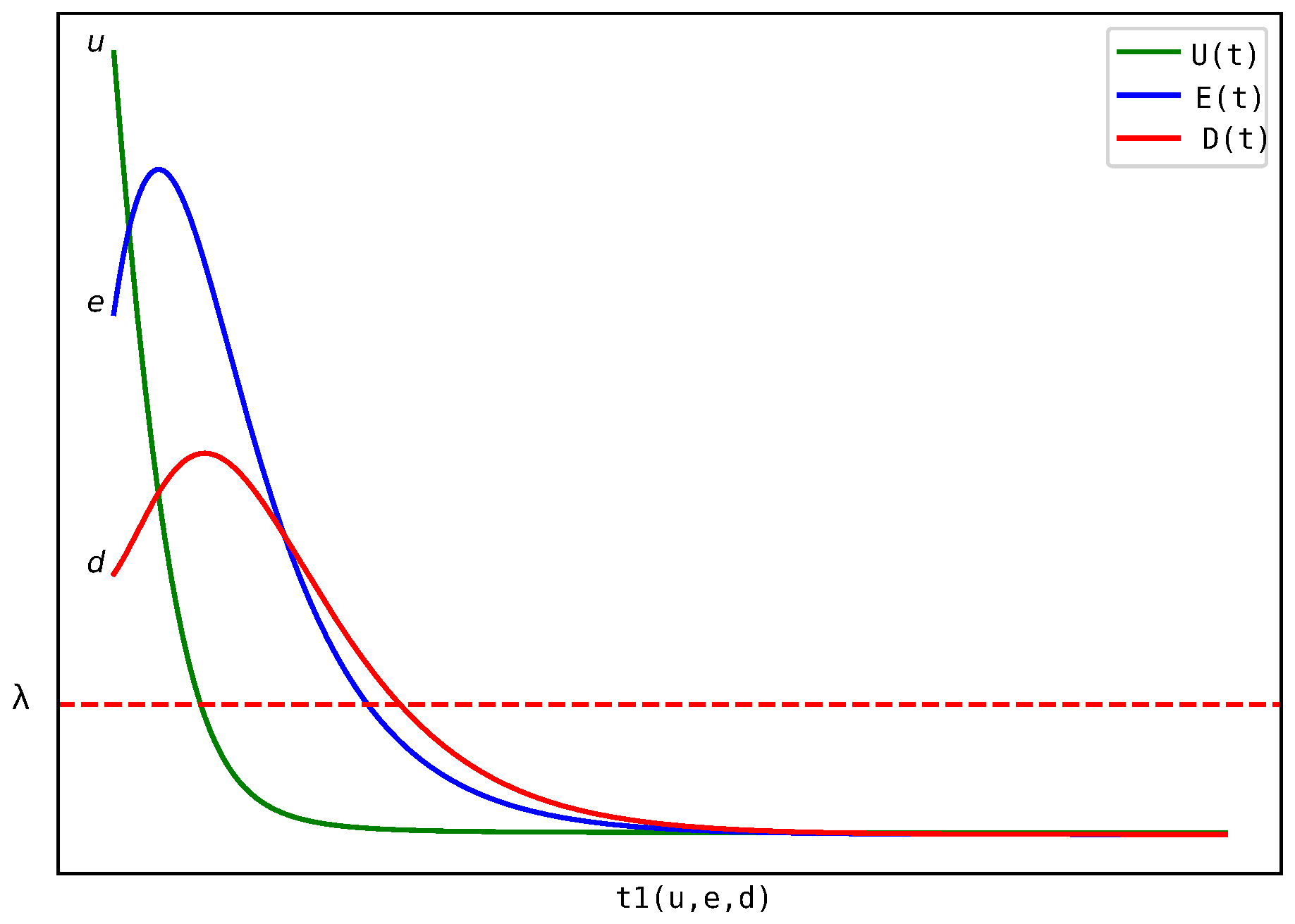
Figure 1 illustrates the transition time $t_1$, defined as the first instance when the number of distressed banks falls below a threshold $\lambda$. This represents the onset of recovery or risk containment. The figure highlights how $t_1$ varies with the initial distribution of undistressed and distressed banks. In practical terms, a larger $t_1$ indicates prolonged systemic distress, underscoring the importance of early intervention when the system begins with high distress levels or limited resilience.

We use the notation $t_1\ge 0$ to denote the initial point at which the value of $D\left(t\right)$ falls below the threshold $\lambda$, indicating a reduction in distressed banks. Additionally, there exists a time interval $t_2\ge 0$ during which $U\left(t\right)$ exhibits a decreasing trend over the interval $[t_2,\infty )$.

Considering that E and D are positive functions and that $\dot{E}\left(t\right)+\dot{D}\left(t\right)=(\beta U\left(t\right)-\gamma )D\left(t\right)$, we can define $t_2$ as the first time point t when the number of undistressed banks falls below a certain threshold, specifically when $U\left(t\right)\le \frac{\gamma }{\beta }$, which is determined by the ratio of recovery and distressed rates. It should be noted that our analysis will focus on understanding how the times $t_1$ and $t_2$, referred to earlier, are influenced by the initial conditions, namely the values of $U\left(0\right)$ and $D\left(0\right)$. 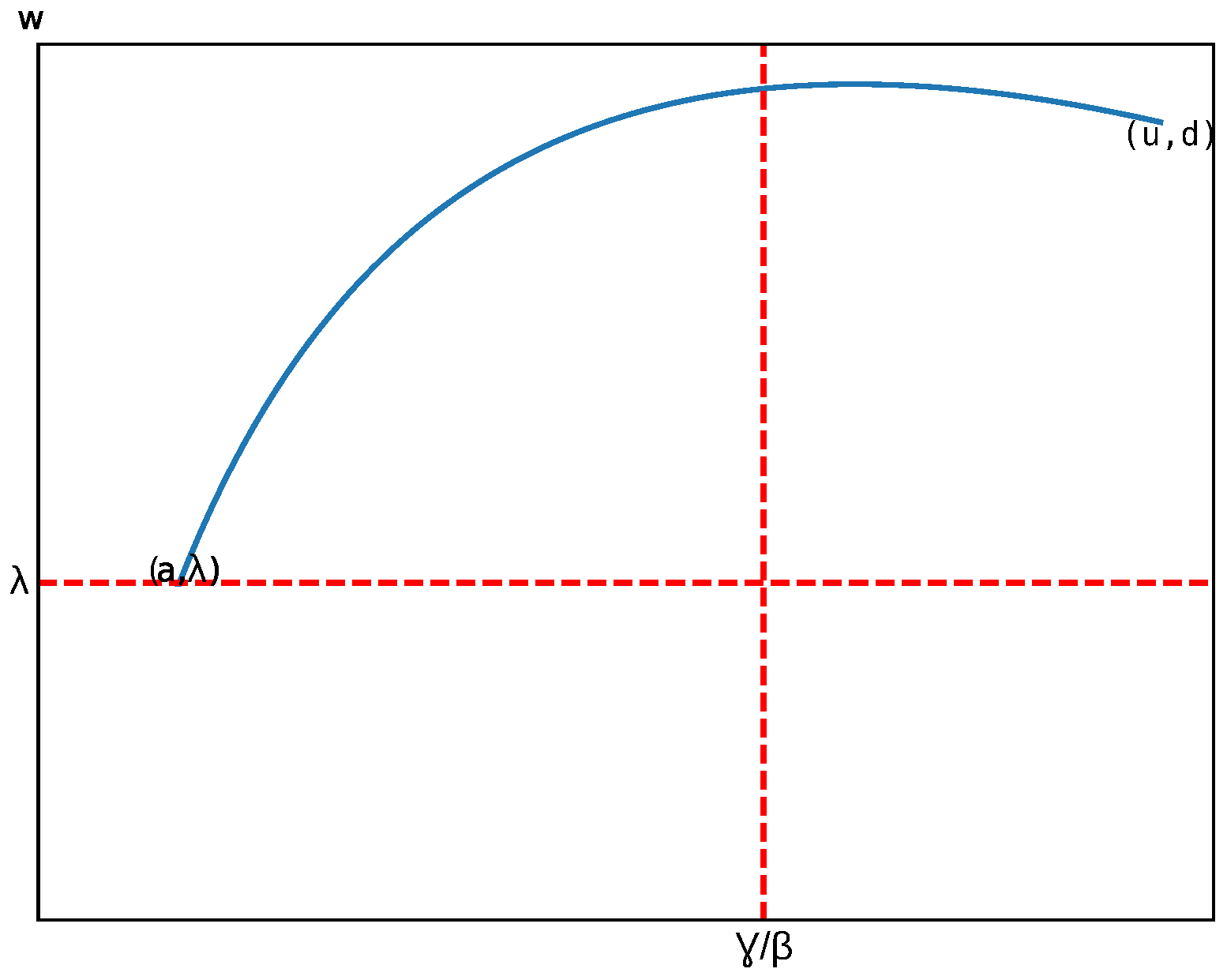To begin, let us establish a threshold value denoted as $\lambda >0$ and examine the function:

$$t_1(u,e,d):=inf\{t>0:D\left(t\right)\le \lambda \}$$

(4)

In this context, U, E, and D represent solutions to Equation (1) with initial conditions $U\left(0\right)=u$, $E\left(0\right)=e$, and $D\left(0\right)=d$ (see Figure 1). Since $t_1(u,e,d)=0$ when $0\le d<\lambda$, our focus will be on the values of $t_1(u,e,d)$ when $u\ge 0$, $e\ge 0$ and $d\ge \lambda$. It is worth noting that $t_1$ exhibits smooth behavior in the domain $(0,\infty )\times (0,\infty )\times (\lambda ,\infty )$ and satisfies the following partial differential equation (PDE):

$$\beta ud{\partial }_u{t}_1+(\sigma e-\beta ud){\partial }_e{t}_1+(\gamma d-\sigma e){\partial }_d{t}_1=1$$

(5)

together with the boundary condition

$$t_1(u,e,\lambda )=0,u\in \left[0,\frac{\gamma }{\beta }\right].$$

(6)

Furthermore, we will utilize $\psi$ as defined in Equation (3) to construct a representation formula for $t_1$. In pursuit of this objective, it is worth observing that for $u>0$, $e>0$, and $d\ge \lambda$, there exists a distinct function $a(u,d)\in (0,\frac{\gamma }{\beta }]$ for which $\psi (u,d)=\psi \left(a\right(u,d),\lambda )$.

Figure 2 shows the transition time $t_2$, which marks the point when the number of undistressed banks drops below a critical threshold $\gamma /\beta$, signaling the emergence of systemic instability. Smaller values of $t_2$ reflect a fragile system likely to deteriorate rapidly, even if initially stable. This has direct relevance for regulators, as $t_2$ serves as an early-warning indicator for timing preventive measures. Together, the figures offer a temporal lens on systemic risk, quantifying both how long recovery might take ($t_1$) and how quickly instability may emerge ($t_2$), depending on the system’s initial state.

The model incorporates two critical thresholds that carry important regulatory meaning in the context of banking stability. The distress tolerance level threshold ($\lambda$) represents a regulatory or risk management benchmark for the maximum acceptable number of distressed banks. When the number of distressed banks falls below $\lambda$, the banking system is viewed as having moved out of crisis conditions and into a phase of stabilization. The second threshold is the resilience threshold ($\gamma /\beta$), which defines the minimum proportion of undistressed banks needed to maintain system-wide resilience. Dropping below $\gamma /\beta$ suggests that the banking network can no longer absorb shocks effectively, signaling heightened systemic fragility and the need for immediate policy action.

3. First Instance of Distress Below Fixed Threshold

Identifying the first time at which the number of distressed banks falls below a specified threshold is of critical importance in the assessment of systemic risk. Economically, this point reflects the onset of stabilization in the banking system—when distress propagation begins to subside, and confidence, interbank lending, and liquidity conditions are likely to improve. Understanding this transition time provides valuable guidance for regulators in determining the appropriate duration and intensity of policy interventions during periods of financial stress. Thus, this section focuses on demonstrating the validity of Theorem 1. We start with a basic upper limit estimation for the variable $t_1$.

In Lemma 1, we provide an upper bound for the time $t_1$ at which the number of distressed banks first falls below a critical threshold $\lambda$. It gives an estimate of how long the distress may persist based solely on the initial conditions. This is crucial for regulators seeking worst-case estimates for intervention timelines.

Lemma 1.

For all non-negative values of $u\ge 0$, $e\ge 0$, and d greater than or equal to λ, the following inequality holds:

$$t_1(u,e,d)\le \frac{u+e+d}{\gamma \lambda }$$

Proof. 

Let $U,E,D$ represent the solutions of the UEDR ODE (1) under the initial conditions $U\left(0\right)=u$, $E\left(0\right)=e$, and $D\left(0\right)=d$.

As $\frac{d}{dt}(U+E+D)\left(t\right)=-\gamma D\left(t\right)$, we can write the following:

$${\int }_0^t\gamma D\left(\tau \right)d\tau +U\left(t\right)+E\left(t\right)+D\left(t\right)=u+e+d.$$

By selecting a time value $t=t_1(u,e,d)$ and recognizing that $D\left(\tau \right)\ge \lambda$ for $0\le \tau \le t_1(u,e,d)$, we obtain the following:

$$t_1(u,e,d)\gamma \lambda \le {\int }_0^{t_1(u,e,d)}\gamma D\left(\tau \right)d\tau \le u+e+d$$

□

Subsequently, it can be noted that D consistently decreases as it approaches the threshold value $\lambda$.

In Lemma 2, we show that the number of distressed banks is decreasing at the transition time $t_1$. This confirms that $t_1$ indeed marks the beginning of a consistent decline in distress, validating its interpretation as the onset of recovery.

Lemma 2.

Assuming u is greater than zero, e is greater than zero, and d is greater than λ, and given that U, E, and D represent the solutions of (1) with initial conditions $U\left(0\right)=u$, $E\left(0\right)=e$, and $D\left(0\right)=d$, we can conclude that the derivative of $D\left(t_1(u,e,d)\right)$ is negative, i.e.,

$$\dot{D}\left(t_1(u,e,d)\right)<0.$$

Proof. 

Given the equation $\dot{E}\left(t\right)+\dot{D}\left(t\right)=(\beta U\left(t\right)-\gamma )D\left(t\right)$, our goal is to establish the following inequality:

$$\beta U\left(t_1(u,e,d)\right)-\gamma <0$$

(7)

If $\beta u\le \gamma$, then $\beta U\left(t\right)<\gamma$ holds for all $t>0$ due to the decreasing nature of function U. As a result, (7) is satisfied for $t=t_1(u,e,d)$. Conversely, if $\beta u>\gamma$, then function D exhibits an increasing trend within the interval $[0,t_2(u,e,d)]$, and

$$\beta U\left(t_2(u,e,d)\right)-\gamma =0.$$

Specifically, for $D\left(t_2(u,e,d)\right)\ge d>\lambda$, it follows that $t_2(u,e,d)<t_1(u,e,d)$. Since U exhibits a decreasing trend,

$$\beta U\left(t_1(u,e,d)\right)-\gamma <\beta U\left(t_2(u,e,d)\right)-\gamma =0.$$

□

Remark 1.

Given that $t_2(u,e,d)=0$ within the domain $u\in [0,\gamma /\beta ]$, $e>0$, and $d>0$, this proof also establishes that

$$t_2(u,e,d)\le t_1(u,e,d)$$

holds true for all $u\ge 0$, $e>0$, and $d\ge \lambda$.

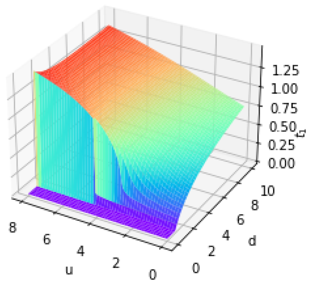
While Figure 3 provides numerical approximations of the function $t_1(u,e,d)$, its significance lies in validating the theoretical results established in Theorem 1. The smooth behavior and boundedness of $t_1$ observed numerically align with its proven continuity and differentiability properties. From a practical standpoint, these simulations help illustrate how different levels of initial distress and exposure can influence the timing of systemic recovery.

In the proof presented for Theorem 1 hereafter, we will utilize the dynamics described by the UEDR ODE (1). This can be represented as the following mapping:

$$\Phi :{[0,\infty )}^4\to {[0,\infty )}^2;(u,e,d,t)\mapsto (U\left(t\right),D\left(t\right))$$

Here, $U,E,D$ signify the solutions to (1) with initial conditions $U\left(0\right)=u$, $E\left(0\right)=e$, and $D\left(0\right)=d$. To simplify, we will also denote $\Phi$ as $\left({\Phi }_1,{\Phi }_2,{\Phi }_3\right)$ so that

$${\Phi }_1(u,e,d,t)=U\left(t\right),{\Phi }_2(u,e,d,t)=E\left(t\right)\mathrm{and}{\Phi }_3(u,e,d,t)=D\left(t\right)$$

It is standard practice to confirm the continuity of $\Phi$. Additionally, it can be demonstrated that $\Phi :{(0,\infty )}^4\to {[0,\infty )}^2$ is indeed a differentiable function.

A key outcome related to the variable $t_1$ is presented below.

Theorem 1.

The function $t_1$ as defined in Equation (4) exhibits the subsequent characteristics.

(i) 

$t_1$ exhibits continuity over the intervals $[0,\infty )\times [0,\infty )\times [\lambda ,\infty )$ and possesses smoothness within $(0,\infty )\times (0,\infty )\times (\lambda ,\infty )$.

(ii) 

$t_1$ represents the sole solution to (5) within the domain $(0,\infty )\times (0,\infty )\times (\lambda ,\infty )$ while conforming to the boundary condition (6).

(iii) 

For every $u>0$, $e>0$ and $d\ge \lambda$, the following equation holds:

$$t_1(u,e,d)={\int }_{a(u,d)}^u\frac{ds}{\beta s\left(\frac{\alpha \gamma }{\beta }lns-\alpha s+\psi (u,d)\right)}$$

(8)

Proof. 

(i) Assuming $u^k\ge 0$, $e^k\ge 0$, and $d^k\ge \lambda$, where $u^k$ approaches u, $e^k$ approaches e, and $d^k$ approaches d as k tends to infinity. According to Lemma 1, $t_1\left(u^k,e^k,d^k\right)$ remains within certain limits. Consequently, we can choose a specific subsequence $t_1\left(u^{k_j},e^{k_j},d^{k_j}\right)$ such that

$$t:=\underset{k\to \infty }{lim\; inf}{t}_1\left(u^k,e^k,d^k\right)=\underset{j\to \infty }{lim}{t}_1\left(u^{k_j},e^{k_j},d^{k_j}\right)$$

Based on the definition of $t_1$, we can further observe that

$${\Phi }_3\left(u^k,e^k,d^k,t_1\left(u^k,e^k,d^k\right)\right)=\lambda$$

(9)

For every natural number k. Given the continuity of ${\Phi }_2$, we can let $k=k_j\to \infty$ in Equation (9) to obtain

$${\Phi }_3(u,e,d,t)=\lambda$$

Given that $d\ge \lambda$, it follows that

$$t_1(u,e,d)\le t=\underset{k\to \infty }{lim\; inf}{t}_1\left(u^k,e^k,d^k\right)$$

Furthermore, we have the option to select an alternate subsequence, denoted as $t_1(u^{k_{\ell }},e^{k_{\ell }},d^{k_{\ell }})$, where

$$v:=\underset{k\to \infty }{lim\; sup}{t}_1\left(u^k,e^k,d^k\right)=\underset{\ell \to \infty }{lim}{t}_1\left(u^{k_{\ell }},e^{k_{\ell }},d^{k_{\ell }}\right)$$

The same argument presented above yields the following equation:

$${\Phi }_3(u,e,d,v)=\lambda$$

If d is greater than $\lambda$ or if $0\le u\le \frac{\gamma }{\beta }$, and d equals $\lambda$, then $t_1$ represents the unique time $\tau$ that satisfies ${\Phi }_3(u,e,d,\tau )=\lambda$. In either situation, s equals $t_1(u,e,d)$. Alternatively, if u is greater than $\frac{\gamma }{\beta }$ and d equals $\lambda$, then the function $\tau \mapsto {\Phi }_3(u,e,d,\tau )$ starts at $d=\lambda$, increases for a certain period, and then decreases to 0 as $\tau$ approaches infinity. It is necessary that either s equals 0 and is less than or equal to $t_1(u,e,d)$ or s equals $t_1(u,e,d)$. Consequently, in all situations,

$$s=\underset{k\to \infty }{lim\; sup}u\left(u^k,e^k,d^k\right)\le t_1(u,e,d)$$

Therefore,

$$t_1(u,e,d)=\underset{k\to \infty }{lim}u\left(u^k,e^k,d^k\right)$$

This implies that $t_1$ exhibits continuity over the intervals $[0,\infty )\times [0,\infty )\times [\lambda ,\infty )$. Assuming $u>0$, $e>0$ and $d>\lambda$ and remembering that ${\Phi }_3(u,e,d,t_1(u,e))=\lambda$. By Lemma 2,

$${\partial }_t{\Phi }_3(u,e,d,t_1(u,e,d))<0$$

As ${\Phi }_3$ exhibits smoothness within a local vicinity of $(u,e,d,t_1(u,e,d))$, the application of the implicit function theorem leads to the conclusion that $t_1$ demonstrates smoothness within a local vicinity of $(u,e,d)$. Consequently, we deduce that $t_1$ is smooth within the region $(0,\infty )\times (0,\infty )\times (\lambda ,\infty )$.

(ii) Consider $u>0$, $e>0$, and $z>\lambda$, where $U,E,D$ represent the solutions of (1) with initial conditions $U\left(0\right)=u$, $E\left(0\right)=e$, and $D\left(0\right)=d$. Note that for every $0\le t<t_1(u,e,d)$,

$$\begin{array}{cc}\hfill t_1(U\left(t\right),E\left(t\right),D\left(t\right))& =inf\{\tau >0:D(t+\tau )\le \lambda \}\hfill \\ & =inf\{\tau :D(t+\tau )\le \lambda \mathrm{and}\tau >0\}\hfill \\ & =inf\{v-t:D(v)\le \lambda \mathrm{and}v>t\}\hfill \\ & =inf\{v:D(v)\le \lambda \mathrm{and}v>t\}-t\hfill \\ & =inf\{v>t:D(v)\le \lambda \}-t\hfill \\ & =t_1(u,e,d)-t\hfill \end{array}$$

The initial equality above is a consequence of the existence of a sole solution to the UEDR ODE; the last equality is a result of our assumption that $t<t_1(u,e,d)$. Hence,

$$\begin{array}{cc}\hfill 1& =-\frac{d}{dt}{t}_1(U\left(t\right),E\left(t\right),D\left(t\right)){|}_{t=0}\hfill \\ & =[\beta U\left(t\right)D\left(t\right){\partial }_u{t}_1(U\left(t\right),E\left(t\right),D\left(t\right))+(\sigma E\left(t\right)-\beta U\left(t\right)D\left(t\right)){\partial }_e{t}_1(U\left(t\right),E\left(t\right),D\left(t\right))\hfill \\ & +(\gamma D\left(t\right)-\sigma E\left(t\right)){\partial }_d{t}_1(U\left(t\right),E\left(t\right),D\left(t\right))]{|}_{t=0}\hfill \\ & =\beta ud{\partial }_u{t}_1(u,e,d)+(\sigma e-\beta ud){\partial }_e{t}_1(u,e,d)+(\gamma d-\sigma e){\partial }_d{t}_1(u,e,d).\hfill \end{array}$$

We conclude that $t_1$ satisfies Equation (5). Consider w as a solution to (5) that complies with the boundary condition (6). Note

$$\begin{array}{cc}\hfill \frac{d}{dt}w(U\left(t\right),E\left(t\right),D\left(t\right))& =-[\beta U\left(t\right)D\left(t\right){\partial }_{u}w(U\left(t\right),E\left(t\right),D\left(t\right))+(\sigma E\left(t\right)-\beta U\left(t\right)D\left(t\right))\hfill \\ & {\partial }_{e}w(U\left(t\right),E\left(t\right),D\left(t\right)+(\gamma D\left(t\right)-\sigma E\left(t\right)){\partial }_{d}w(U\left(t\right),E\left(t\right),D\left(t\right))]=-1\hfill \end{array}$$

for $0\le t<t_1(u,e,d)$. If we integrate this equation over the interval from $t=0$ to $t=t_1(u,e,d)$, it results in

$$w(U\left(t_1(u,e,d)\right),E\left(t_1(u,e,d)\right),D\left(t_1(u,e,d)\right))-w(u,e,d)=-t_1(u,e,d).$$

Given that $D\left(t_1(u,e,d)\right)=\lambda$ and $\beta U\left(t_1(u,e,d)\right)\le \gamma$, with $w(U\left(t_1(u,e,d)\right),\lambda )=0$, we can conclude that $w(u,e,d)=t_1(u,e,d)$. Consequently, $t_1$ stands as the sole solution to the PDE (5) while meeting the boundary condition (11).

(iii) Assume that $u>0$, $e>0$, and either $d>\lambda$ or $u>\frac{\gamma }{\beta }$, $e>0$, and $d=\lambda$. We should note that $a=a(u,d)\in (0,\frac{\gamma }{\beta }]$ represents the unique solution to the equation:

$$\psi (u,d)=\psi (a,\lambda )$$

Furthermore, it can be readily verified that

$$\frac{\alpha \gamma }{\beta }lns-\alpha s+\psi (u,d)>\lambda$$

holds true for $a<s<u$. Refer to Figure 2 for an illustrative example. Since $t_1$ solves the PDE (5),

$$\begin{array}{cc}& \frac{d}{ds}{t}_1\left(s,e,\frac{\alpha \gamma }{\beta }lns-\alpha s+\psi (u,d)\right)\hfill \\ & ={\left.\frac{\beta sd{\partial }_u{t}_1(s,e,d)+(\sigma e-\beta sd){\partial }_e{t}_1(s,e,d)+(\gamma d-\sigma e){\partial }_d{t}_1(s,e,d)}{\beta sd}\right|}_{d=\frac{\alpha \gamma }{\beta }lns-\alpha s+\psi (u,d)}\hfill \\ & =\frac{1}{\beta s\left(\frac{\alpha \gamma }{\beta }lns-\alpha s+\psi (u,d)\right)}\hfill \end{array}$$

for $a<s<u$. If we integrate from $s=a$ to $s=u$ and apply the boundary condition (6), we obtain the following:

$$t_1(u,e,d)={\int }_a^u\frac{ds}{\beta s(\frac{\alpha \gamma }{\beta }lns-\alpha s+\psi (u,d))}$$

□

It follows from the dynamics of the model that the number of distressed banks cannot begin to decline before reaching its peak—the maximum value of $D\left(t\right)$ over the course of the contagion. This peak occurs when the rate of change of distress satisfies $\dot{D}\left(t\right)=0$. From the governing equations, this condition is met precisely when the number of undistressed banks equals the ratio of the recovery rate to the transmission rate, i.e., $U\left(t\right)=\frac{\gamma }{\beta }$. Consequently, the distress level $D\left(t\right)$ begins to decrease if and only if $U\left(t\right)\le \frac{\gamma }{\beta }$. This observation implies the existence of a critical time $t_2\ge 0$ beyond which the number of distressed banks declines monotonically, i.e., $D\left(t\right)$ is decreasing for all $t\ge t_2$. This result rigorously confirms that $t_1$ is well defined, continuous, and uniquely determined by the system’s initial conditions. Understanding these properties is essential for designing reliable early-warning indicators that inform regulators when systemic risk containment begins.

The mathematical results established in this section (particularly the continuity, uniqueness, and explicit representation of the transition time $t_1$) provide a rigorous foundation for estimating when systemic distress in the banking sector begins to decline. For policymakers and regulators, this time point serves as a dynamic indicator for assessing the effectiveness of crisis containment measures. By understanding how $t_1$ varies with the initial composition of undistressed, exposed, and distressed banks, decision-makers can better anticipate the timing of recovery, allocate intervention resources more efficiently, and design threshold-based triggers for regulatory action during financial crises.

4. First Instance Undistress Falls Below the Threshold

We will now highlight the necessary adjustments from the preceding section to establish Theorem 2 concerning $t_2$. It is important to begin by observing that $t_2$ exhibits local boundedness within $[\frac{\gamma }{\beta },\infty )\times (0,\infty )\times (0,\infty )$.

Lemma 3.

For all values of $u\ge \frac{\gamma }{\beta }$, $e>0$ and $d>0$,

$$t_2(u,e,d)\le \frac{lnu-ln(\gamma /\beta )}{\beta d}$$

Proof. 

Consider the solutions $U,E,D$ of (1) with initial conditions $U\left(0\right)=u$, $E\left(0\right)=e$, and $D\left(0\right)=d$. As $D\left(t\right)$ exhibits monotonic growth for $t\in [0,t_2(u,e,d)]$, it follows that $D\left(t\right)\ge d$ for $t\in [0,t_2(u,e,d)]$. Referring to Equation (2),

$$\frac{\gamma }{\beta }=U\left(t_2(u,e,d)\right)=x{e}^{-\beta {\int }_0^{t_2(u,e,d)}D\left(\tau \right)d\tau }\le u{e}^{-\beta d{t}_2(u,e,d)}.$$

By applying the natural logarithm and rearranging the equation, we obtain the desired result: $t_2(u,e,d)\le \frac{lnu-ln(\gamma /\beta )}{\beta d}$. □

Lemma 3 provides an upper bound for $t_2$, the time when the number of undistressed banks drops below the critical stability threshold $\gamma /\beta$. It helps assess how quickly systemic instability may emerge after a shock.

The subsequent claim can be deduced because the function $U\left(t\right)$ exhibits a decreasing trend whenever $D\left(t\right)$ is initially positive. The primary purpose of introducing this lemma is to draw a parallel with Lemma 2.

Lemma 4.

If u is greater than or equal to $\frac{\gamma }{\beta }$, and both e and d are greater than zero, and if U, E, and D represent the solution to Equation (1) with initial conditions $U\left(0\right)=u$, $E\left(0\right)=e$, and $D\left(0\right)=d$, then the derivative of $U\left(t_2(u,e,d)\right)$ is negative.

In Lemma 4, we establish that at time $t_2$, the number of undistressed banks is decreasing. This validates that $t_2$ marks the beginning of systemic fragility, reinforcing its role as an early-warning indicator.

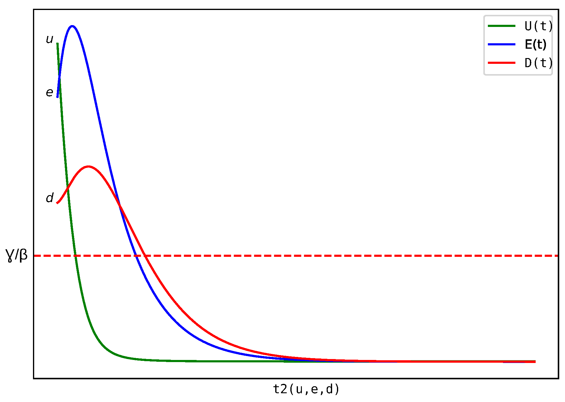
Next, we study

$$t_2(u,e,d):=inf\{t>0:U\left(t\right)\le \frac{\gamma }{\beta }\}$$

(10)

for $e\ge 0$ and $d\ge 0$. Once more, we are considering U, E, and D as the solution triplet for the UEDR ODE (1), where the initial conditions are $U\left(0\right)=u$, $E\left(0\right)=e$, and $D\left(0\right)=d$ (Figure 4). Given that

$$\left\{\begin{array}{c}{t}_2(u,e,d)=0\mathrm{for}0\le u\le \frac{\gamma }{\beta }\mathrm{and}\hfill \\ t_2(u,e,0)=\infty \mathrm{for}u>\frac{\gamma }{\beta },\hfill \end{array}\right.$$

we concentrate on evaluating the values of $t_2(u,e,d)$ within the parameter space defined as $u>\frac{\gamma }{\beta }$, $e>0$, and $d>0$. Additionally, it is important to observe that in cases where $d>0$, the function $t_2(u,e,d)$ captures the initial instance at which $D\left(t\right)$ commences its decline. The methodologies we employ to establish the validity of Theorem 1 can similarly be extended to analyze $t_2$. Notably, $t_2$ adheres to the same partial differential equation (PDE) as $t_1$, with corresponding boundary conditions.

$$t_2(\frac{\gamma }{\beta },e,d)=0,d\in (0,\infty ).$$

(11)

Figure 4 illustrates the trajectories of undistressed, exposed, and distressed banks under a given initial conditions, highlighting the point in time when the undistressed population falls below the threshold $\gamma /\beta$. This threshold marks the system’s loss of resilience, beyond which distress begins to decline due to insufficient undistressed banks to sustain contagion. In practical terms, this corresponds to the moment when the financial system becomes critically fragile, indicating the need for immediate regulatory intervention. The dynamics depicted reinforce the importance of monitoring early shifts in the undistressed population to anticipate the tipping point of systemic vulnerability.

Theorem 2.

The function $t_2$ as described in Equation (11) exhibits the subsequent characteristics.

(i) 

$t_2$ is a continuous function over the domain $[\frac{\gamma }{\beta },\infty )\times (0,\infty )\times (0,\infty )$ and exhibits smooth behavior within the region $(\frac{\gamma }{\beta },\infty )\times (0,\infty )\times (0,\infty )$.

(ii) 

$t_2$ represents the sole solution to (5) within the region $(\frac{\gamma }{\beta },\infty )\times (0,\infty )\times (0,\infty )$ while adhering to the boundary condition (11).

(iii) 

For all values of u greater than or equal to $\frac{\gamma }{\beta }$, with e and d both being positive,

$$t_2(u,e,d)={\int }_{\frac{\gamma }{\beta }}^u\frac{ds}{\beta s\left(\frac{\alpha \gamma }{\beta }lns-\alpha s+\psi (u,d)\right)}$$

(12)

We observe that a similar expression (12) has previously been derived in the context of the SIR (Susceptible–Infected–Recovered) model, as demonstrated, for instance, in references such as [15,21]. What distinguishes our research is the use of this formula in the context of the UEDR model, where it is regarded as a function reliant on initial conditions denoted as u, e, and d. We further characterize this function as a solution to the partial differential Equation (5), subject to specific boundary conditions. Furthermore, we leverage this formula in conjunction with (1) to provide precise estimations for $t_1(u,e,d)$ and $t_2(u,e,d)$ under conditions where the sum $u+e+d$ attains large values.

Proof. 

Now that we have confirmed Lemmas 3 and 4, we can follow a nearly identical approach as outlined in the preceding section to establish the conclusion of Theorem 2. Therefore, we will forego presenting the proof. □

Theorem 2 characterizes the behavior of the time $t_2$, which marks the onset of systemic instability as undistressed banks fall below a resilience threshold. The theorem ensures that $t_2$ is mathematically robust and responsive to initial banking conditions, providing a theoretical foundation for assessing when the banking system becomes highly vulnerable to contagion. Such insights are crucial for timing preventive interventions and liquidity support measures.

The results presented in this section provide a rigorous mathematical characterization of the time $t_2$, which marks the first instance undistressed banks fall below the threshold. By proving the existence, continuity, and explicit representation of $t_2$, we establish a formal tool for identifying when the financial system transitions from a stable to a vulnerable state. For banking regulators and policymakers, $t_2$ offers a forward-looking indicator to support the timing of macroprudential interventions, such as capital buffer adjustments or liquidity injections. Understanding how $t_2$ evolves under different initial conditions enables more responsive, data-informed risk monitoring. In the next section, we extend this analysis by examining the limiting behavior of $t_1$ and $t_2$ under large-scale systemic shocks, further reinforcing their use in stress testing and early-warning frameworks.

5. Limiting Behaviors

We compute approximations for $t_1(u,e,d)$ and $t_2(u,e,d)$, which are essential for demonstrating Theorem 3. Initially, we establish both an upper and lower limit for $t_1$.

In the analysis that follows, we make use of integrals and limiting behavior to characterize the timing and evolution of systemic distress. The integral expressions accumulate the effects of contagion over time, accounting for how initial conditions (such as the number of undistressed or distressed banks) influence the spread or recovery of risk. Rather than focusing on a single point in time, these integrals capture the cumulative impact of dynamic interactions across the banking network. Similarly, the limit expressions describe what happens when the initial number of distressed or undistressed banks becomes very large. In practical terms, these limits help us understand the behavior of the financial system under extreme stress scenarios, such as widespread insolvency or liquidity collapse. They offer insights into how long distress might persist or how quickly vulnerability may emerge in large-scale crises.

The limiting behaviors of $t_1(u,e,d)$ and $t_2(u,e,d)$ analyzed in this section directly address the core objective outlined in the introduction: to quantify the timing of systemic risk containment and the onset of instability in relation to the initial state of the banking system. These results, derived from the UEDR model, reveal how critical transition times behave under extreme conditions—such as when distress is widespread or when undistressed banks are few. This asymptotic analysis strengthens the model’s predictive capability and offers valuable insights for stress-testing frameworks. It confirms that as systemic stress intensifies (i.e., as $u+e+d\to \infty$), the time to containment ($t_1$) grows proportionally, while the time to instability ($t_2$) shrinks, guiding regulators on the urgency and duration of intervention required under severe financial shocks.

Lemma 5.

In the case where u is non-negative, e is non-negative, and d is greater than or equal to λ, then

$$t_1(u,e,d)\ge \frac{1}{\gamma }ln\left(\frac{u+e+d}{\gamma /\beta +\lambda }\right)$$

(13)

If $u\in [0,\gamma /\beta )$, $e\ge 0$ and $d\ge \lambda$, then

$$t_1(u,e,d)\le \frac{ln(e+d)/\lambda )}{(\gamma -\beta u)}$$

(14)

Proof. 

Consider the following expression:

$$w(u,e,d)=\frac{1}{\gamma }ln\left(\frac{u+e+d}{\gamma /\beta +\lambda }\right).$$

It is noteworthy that when $u\ge 0$, $e\ge 0$ and $d\ge \lambda$, the following holds:

$$\beta ud{\partial }_{u}w+(\sigma e-\beta ud){\partial }_{e}w+(\gamma d-\sigma e){\partial }_{d}w=\frac{1}{\gamma }\frac{\beta ud+(\sigma e-\beta ud)+(\gamma d-\sigma e)}{u+e+d}=\frac{d}{u+e+d}\le 1$$

Now, consider $u\ge 0$, $e\ge 0$, and $d\ge \lambda$, and assume that $U,E,D$ represents the solution of (1) with initial conditions $U\left(0\right)=u$, $E\left(0\right)=e$, and $D\left(0\right)=d$. Based on the calculations above,

$$\begin{array}{cc}\hfill \frac{d}{dt}w(U\left(t\right),E\left(t\right),D\left(t\right))=& -[\beta U\left(t\right)D\left(t\right){\partial }_{u}w(U\left(t\right),E\left(t\right),D\left(t\right))+(\sigma E\left(t\right)-\beta U\left(t\right)){\partial }_{e}w(U\left(t\right),E\left(t\right),D\left(t\right))\hfill \\ \hfill & +(\gamma D\left(t\right)-\sigma E\left(t\right)){\partial }_{d}w(U\left(t\right),E\left(t\right),D\left(t\right))]\ge -1\hfill \end{array}$$

for $0\le t\le t_1(u,e,d)$. When we integrate this inequality over the interval from $t=0$ to $t=t_1(u,e,d)$, we obtain the following result:

$$w(U\left(t_1(u,e,d)\right),y,\lambda )-w(u,e,d)\ge -t_1(u,e,d)$$

(15)

Since $U\left(t_1(u,e,d)\right)\le \frac{\gamma }{\beta }$

$$w(U\left(t_1(u,e,d)\right),y,\lambda )=\frac{1}{\gamma }ln\left(\frac{S\left(t_1(u,e,d)\right)+y+\lambda }{\gamma /\beta +\lambda }\right)\le 0$$

When Equation (15) is combined with this, it results in $t_1(u,e,d)\ge w(u,e,d)$. As a consequence, we can deduce (13). Now, let us assume that $\beta u<\gamma$, $e>0$, and $d>\lambda$ based on Equation (1),

$$\begin{array}{cc}& \frac{d\left(E\right(t)+D(t\left)\right)}{dt}=(\beta U\left(t\right)-\gamma )D\left(t\right)\hfill \\ & \frac{d\left(E\right(t)+D(t\left)\right)}{D\left(t\right)}=(\beta U\left(t\right)-\gamma )dt\Rightarrow \frac{d\left(E\right(t)+D(t\left)\right)}{E\left(t\right)+D\left(t\right)}\le (\beta U\left(t\right)-\gamma )dt\hfill \\ & E(t_1(u,e,d)+D(t_1(u,e,d)\le (y+z)e^{{\int }_0^{t_1(u,e,d)}(\beta U\left(\tau \right)-\gamma )d\tau }\hfill \\ & \lambda =D(t_1(u,e,d)\le (y+z)e^{{\int }_0^{t_1(u,e,d)}(\beta U\left(\tau \right)-\gamma )d\tau }\le (y+z)e^{(\beta u-\gamma )t_1(u,e,d)}\hfill \end{array}$$

By applying the natural logarithm and reordering, we obtain Equation (14). □

Lemma 5 provides lower and upper bounds for $t_1$, capturing the earliest and most delayed possible times for risk containment. These bounds are important for conducting sensitivity analysis and assessing the temporal range of systemic risk mitigation under varying initial conditions.

Similarly, we can establish practical upper and lower limits for $t_2(u,e,d)$. In doing so, we will leverage the observation that, for every $u>\frac{\gamma }{\beta }$, $e>0$, and $d>0$,

$$g\left(s\right)=\frac{\alpha \gamma }{\beta }lns-\alpha s+\psi (u,d)$$

exhibits concavity over the range of $\frac{\gamma }{\beta }\le s\le u$. This implies

$$\begin{array}{cc}\hfill g\left(s\right)\ge \frac{g\left(\frac{\gamma }{\beta }\right)-d}{\frac{\gamma }{\beta }-u}(s-u)+g\left(u\right)& =\left(\frac{\alpha \gamma }{\beta }\frac{lnu-ln(\gamma /\beta )}{u-\gamma /\beta }-\alpha \right)(s-u)+d\hfill \\ \hfill & =\alpha \left(\frac{\gamma }{\beta }\frac{lnu-ln(\gamma /\beta )}{u-\gamma /\beta }-1\right)(s-u)+d\hfill \end{array}$$

(16)

and

$$g\left(s\right)\le g^{\prime }\left(u\right)(s-u)+g\left(u\right)=\alpha \left(\frac{\gamma }{\beta u}-1\right)(d-u)+d$$

(17)

for $\frac{\gamma }{\beta }\le s\le u$.

Lemma 6.

Suppose $u>\frac{\gamma }{\beta }$, $e>0$ and $d>0$. Then

$$t_2(u,e,d)\le \frac{lnu-ln(\gamma /\beta )-lnd+ln\left(\alpha u-\alpha \gamma /\beta +d-\frac{\alpha \gamma }{\beta }(lnu-ln(\gamma /\beta ))\right)}{\beta \left(d+\alpha u\left(1-\frac{\gamma }{\beta }\frac{lnu-ln(\gamma /\beta )}{u-\gamma /\beta }\right)\right)}$$

(18)

$$t_2(u,e,d)\ge \frac{lnu-ln(\gamma /\beta )-lnd+ln\left(\alpha u-\alpha \gamma /\beta +d+\frac{\alpha \gamma }{\beta }\left(\frac{\gamma }{\beta u}-1\right)\right)}{\beta (\alpha u-\alpha \gamma /\beta +d)}$$

(19)

Proof. 

We refer to part (iii) of Theorem 2, which states

$$t_2(u,e,d)={\int }_{\frac{\gamma }{\beta }}^u\frac{ds}{\beta sg\left(s\right)}$$

We also utilize the identity

$$\frac{d}{ds}\frac{lns-ln(cs+f)}{f}=\frac{1}{s(cs+f)}$$

(20)

By Equations (16) and (20), we have

$$\begin{array}{ccc}\hfill t_2(u,e,d)& \le & {\int }_{\frac{\gamma }{\beta }}^u\frac{ds}{\beta s\left(\alpha \left(\frac{\gamma }{\beta }\frac{lnu-ln\frac{\gamma }{\beta }}{u-\frac{\gamma }{\beta }}-1\right)(s-u)+d\right)}\hfill \\ & =& {\left.\frac{lns-ln\left(\alpha \left(\frac{\gamma }{\beta }\frac{lnu-ln\frac{\gamma }{\beta }}{u-\frac{\gamma }{\beta }}-1\right)(s-u)+d\right)}{\beta \left(d+\alpha u\left(1-\frac{\gamma }{\beta }\frac{lnu-ln\frac{\gamma }{\beta }}{u-\frac{\gamma }{\beta }}\right)\right)}\right|}_{s=\frac{\gamma }{\beta }}^{s=u}\hfill \\ & =& \frac{lnu-ln\frac{\gamma }{\beta }-lnd+ln\left(\alpha u-\alpha \frac{\gamma }{\beta }+d-\frac{\alpha \gamma }{\beta }\left(lnu-ln\frac{\gamma }{\beta }\right)\right]}{\beta \left(d+\alpha u\left(1-\frac{\gamma }{\beta }\frac{lnu-ln\frac{\gamma }{\beta }}{u-\frac{\gamma }{\beta }}\right)\right)}\hfill \end{array}$$

Similarly, Equations (17) and (20) give

$$\begin{array}{cc}& t_2\left(u,e,d\right)⩾{\int }_{\frac{\gamma }{\beta }}^u\frac{ds}{\beta s\left(\alpha \left(\frac{\gamma }{\beta }-1\right)(s-u)+d\right)}\hfill \\ & ={\left.\frac{lns-ln\left(\alpha \left(\frac{\gamma }{\beta u}-1\right)(s-u)+d\right)}{\beta \left(\alpha u-\frac{\alpha \gamma }{\beta }+d\right)}\right|}_{s=\frac{\gamma }{\beta }}^{s=u}\hfill \\ & =\frac{lnu-ln\frac{\gamma }{\beta }-lnd+ln\left(\alpha u-\frac{\alpha \gamma }{\beta }+d+\frac{\alpha \gamma }{\beta }\left(\frac{\gamma }{\beta }-1\right)\right)}{\beta \left(\alpha u-\frac{\alpha \gamma }{\beta }+d\right)}\hfill \end{array}$$

□

In Lemma 6, we derive explicit upper and lower bounds for the transition time $t_2$, which denotes the first time the number of undistressed banks falls below the critical threshold $\gamma /\beta$. These bounds are expressed in terms of the model parameters and initial conditions, offering a practical way to estimate how quickly a banking system may transition from a stable state to a distressed state. In regulatory terms, these bounds help determine the window of time available for preventive measures before systemic stress intensifies.

Corollary 1.

For each $\delta >0$,

$$\underset{\underset{u⩾0,e⩾0,d⩾\delta }{u+e+d\to \infty }}{lim}{t}_2(u,e,d)=0$$

(21)

Proof. 

Choose sequence $u_k⩾0,e_k⩾0$ and $d_k⩾\delta$ with $u_k+e_k+d_k\to \infty$ such that

$$\underset{\underset{u⩾0,e⩾0,d⩾\delta }{u+e+d\to \infty }}{lim}sup{t}_2(u,e,d)=\underset{k\to \infty }{lim}{t}_2\left(u_k,e_k,d_k\right)$$

If there exists an infinite sequence of natural numbers $k\in \mathbb{N}$ such that $u_k\le \frac{\gamma }{\beta }$, then it follows that there exists an infinite sequence of corresponding values of k for which $t_2\left(u_k,e_k,d_k\right)=0$ and

$$\underset{k\to \infty }{lim}{t}_2\left(u_k,e_k,d_k\right)=0$$

(22)

Alternatively, we can assume that $u_k>\gamma /\beta$ for all $k\in \mathbb{N}$. Under this condition, inequality (18) implies

$$\begin{array}{cc}& t_2\left(u_k,e_k,d_k\right)\le \frac{ln{u}_k-ln\frac{\gamma }{\beta }-ln{d}_k+ln\left(\alpha u_k-\frac{\alpha \gamma }{\beta }+d_k-\frac{\alpha \gamma }{\beta }\left(ln{u}_k-ln(\gamma /\beta )\right)\right)}{\beta \left(d_k+\alpha u_k\left(1-\frac{\gamma }{\beta }\frac{ln{u}_k-ln\left(\frac{\gamma }{\beta }\right)}{\left(u_k-\frac{\gamma }{\beta }\right)}\right)\right)}\hfill \\ & \mathrm{for}\mathrm{all}k\in \mathbb{N}\hfill \\ & \mathrm{if}{u}_k\to \infty ,\mathrm{then}\frac{\gamma }{\beta }\frac{ln{u}_k-ln\left(\frac{\gamma }{\beta }\right)}{u_k-\frac{\gamma }{\beta }}\le \frac{1}{2}\hfill \end{array}$$

for large k. It implies that

$$\begin{array}{ccc}\hfill t_2\left(u_k,e_k,d_k\right)& \le & \frac{ln{u}_k-ln\frac{\gamma }{\beta }-ln{d}_k+ln\left(\alpha u_k-\frac{\alpha \gamma }{\beta }+d_k-\frac{\alpha \gamma }{\beta }\left(ln{u}_k-ln(\gamma /\beta )\right)\right)}{\beta \left(d_k+\frac{1}{2}\alpha u_k\right)}\hfill \\ & \le & \frac{ln{u}_k-ln\frac{\gamma }{\beta }+ln\left(\frac{\alpha u_k-\frac{\alpha \gamma }{\beta }}{d_k}+1\right)}{\beta \left(d_k+\frac{1}{2}\alpha u_k\right)}\hfill \\ & \le & \frac{ln{u}_k-ln\frac{\gamma }{\beta }+ln\left(\frac{\alpha u_k-\frac{\alpha \gamma }{\beta }}{\delta }+1\right)}{\beta \left(\delta +\frac{1}{2}\alpha u_k\right)}\hfill \end{array}$$

for all large enough k. Hence, the Equation (22) remains valid. As an alternative, we can transition to a subsequence, if required, and assume that $u_k\le c$ holds for all $k\in \mathbb{N}$, with $e_k$ and $d_k$ both converging to infinity. In this case, Lemma 3 provides

$$t_2\left(u_k,e_k,d_k\right)\le \frac{lnc-ln(\gamma /\beta )}{\beta d_k}\to 0$$

Consequently, the Equation (22) is valid in all scenarios, implying that

$$\underset{\begin{array}{c}u+e+d\to \infty \\ x\ge 0,y\ge 0,z\ge \delta \end{array}}{lim\; sup}{t}_2(u,e,d)=0$$

which in consequence, suggests (21). □

This leads now to the following result:

Theorem 3.

Define the function $t_1$ as described in Equation (4) and let $t_2$ be defined by Equation (11). Then, the following limits hold:

$$\underset{\underset{u\ge 0,e\ge 0,d\ge \lambda }{u+e+d\to \infty }}{lim}\frac{t_1(u,e,d)}{\frac{1}{\gamma }ln\left(\frac{u+e+d}{\lambda }\right)}=1$$

(23)

$$\underset{\underset{u\ge \frac{\gamma }{\beta },e>0,d>0}{u+e+d\to \infty }}{lim}\frac{\beta \left(\alpha u-\alpha \gamma /\beta +d\right)}{\left[ln\left(\frac{u}{\gamma /\beta }\right)\left(\alpha \frac{u-\gamma /\beta }{d}+1\right)\right]}{t}_2(u,e,d)=1$$

(24)

From Equation (23), it can be deduced that as $u+e+d\to \infty$, the function $t_1(u,e,d)$ tends toward infinity. This implies that we are essentially examining solutions to the UEDR ODE (1) over extremely extended time intervals. It is worth noting that the limits described in (23) and (24) differ from the conventional large-time asymptotic outcomes for solutions to (1), as they pertain to solutions with diverse initial conditions.

Proof. 

In view of Equation (13),

$$\underset{\begin{array}{c}u+e+d\to \infty \\ u\ge 0\\ e\ge 0,d\ge \lambda \end{array}}{lim\; inf}\frac{t_1(u,e,d)}{\frac{1}{\gamma }ln\left(\frac{u+e+d}{\lambda }\right)}\ge 1$$

It can be deduced that as $u+e+d\to \infty$ with $u\ge 0$, $e\ge 0$, and $d\ge \lambda$, the function $t_1(u,e,d)$ tends towards infinity. Referring to Corollary 1, we can choose a sufficiently large natural number $N\in \mathbb{N}$ such that

$$t_2(u,e,d)<t_1(u,e,d)$$

holds true for all $u+e+d\ge N$ with $u\ge 0$, $e\ge 0$, and $d\ge \lambda$. Assume that $u+e+d\ge N$, where $u\ge 0$, $e\ge 0$, and $d\ge \lambda$. Let us select a time point t such that

$$t_2(u,e,d)<t<t_1(u,e,d)$$

It is important to observe that when t exceeds $t_2(u,e,d)$, the following relationship holds:

$$U\left(t\right)<\frac{\gamma }{\beta }$$

In this context, U, E, and D represent the solutions to the UEDR ODE (1), with initial conditions $U\left(0\right)=u$, $E\left(0\right)=e$, and $D\left(0\right)=d$. By (14), we also have

$$\begin{array}{cc}\hfill t_1(u,e,d)& =t+t_1(U\left(t\right),E\left(t\right),D\left(t\right))\hfill \\ \hfill & \le t+\frac{1}{\gamma -\beta U\left(t\right)}ln\left(\frac{E\left(t\right)+D\left(t\right)}{\lambda }\right)\hfill \\ \hfill & \le t+\frac{1}{\gamma -\beta U\left(t\right)}ln\left(\frac{u+e+d}{\lambda }\right)\hfill \end{array}$$

(25)

Furthermore, we can employ (2) to determine the following:

$$\begin{array}{cc}\hfill U\left(t\right)& =U\left(t_2(u,e,d)\right)e^{-\beta {\int }_{t_2(u,e,d)}^{t}D\left(\tau \right)d\tau }\hfill \\ & =\frac{\gamma }{\beta }{e}^{-\beta {\int }_{t_2(u,e,d)}^{t}D\left(\tau \right)d\tau }\hfill \\ & \le \frac{\gamma }{\beta }{e}^{-\beta \lambda (t-t_2(u,e,d))}\hfill \end{array}$$

In this context, we have employed the condition $D\left(\tau \right)\ge \lambda$ for $\tau \le t<t_1(u,e,d).$ Consequently, we can express it as follows:

$$\gamma -\beta U\left(t\right)\ge \gamma \left(1-e^{-\beta \lambda (t-t_2(u,e,d)})\right)$$

Combining this inequality with (25), we obtain the following result:

$$t_1(u,e,d)\le t+\frac{1}{1-e^{-\beta \lambda (t-t_2(u,e,d)}}\frac{1}{\gamma }ln\left(\frac{u+e+d}{\lambda }\right)$$

Then,

$$\underset{\begin{array}{c}u+e+d\to \infty \\ u\ge 0\\ e\ge 0\\ d\ge \lambda \end{array}}{lim\; sup}\frac{t_1(u,e,d)}{\frac{1}{\gamma }ln\left(\frac{u+e+d}{\lambda }\right)}\le \frac{1}{1-e^{-\beta \lambda t}}$$

We establish (23) as t approaches infinity. □

Theorem 3 analyzes the asymptotic behavior of the critical times $t_1$ and $t_2$ as the overall size of distress in the banking system grows. It provides precise limits that describe how these times behave under extreme stress scenarios. This asymptotic analysis offers important insights for stress-testing frameworks and systemic risk models, especially when evaluating large-scale crises where traditional assumptions may no longer hold.

In the discussion that follows, we will utilize the basic inequalities as expressed in the formulas below:

$$\frac{1}{u}\le \frac{lnu-ln(\gamma /\beta )}{u-\gamma /\beta }\le \frac{\beta }{\gamma },$$

(26)

which are valid for $u>\gamma /\beta$. These results stem from the concave nature of the natural logarithm.

Proof of (24):

Proof. 

Using the upper limit as indicated in Equation (18),

$$\begin{array}{cc}\hfill & \frac{\beta (\alpha u-\alpha \gamma /\beta +d)}{ln\left[\left(\frac{u}{\gamma /\beta }\right)\left(\alpha \frac{u-\gamma /\beta }{e}+1\right)\right]}·t_2(u,e,d)\hfill \\ \hfill & =\frac{\beta (\alpha u-\alpha \gamma /\beta +d)}{lnu-ln(\gamma /\beta )-lnd+ln(\alpha u-\alpha \gamma /\beta +d)}·t_2(u,e,d)\hfill \\ \hfill & \le \frac{\beta (\alpha u+d)}{lnu-ln(\gamma /\beta )-lnd+ln\left(\alpha u-\alpha \gamma /\beta +d-\frac{\alpha \gamma }{\beta }(lnu-ln(\gamma /\beta ))\right)}·t_2(u,e,d)\hfill \\ \hfill & \le \frac{\alpha u+d}{d+\alpha u\left(1-\frac{\gamma }{\beta }\frac{lnu-ln(\gamma /\beta )}{u-\gamma /\beta }\right)}\hfill \\ \hfill & =\frac{1}{1-\frac{\alpha u}{\alpha u+d}\frac{\gamma }{\beta }\left(\frac{lnu-ln(\gamma /\beta )}{u-\gamma /\beta }\right)}.\hfill \end{array}$$

(27)

Certainly, we can choose sequences $u_k>\gamma /\beta$, $e_k>0$, and $d_k>0$ such that $u_k+e_k+d_k\to \infty$ and

$$\underset{\begin{array}{c}u+e+d\to \infty \\ u>\gamma /\beta ,y>0,d>0\end{array}}{lim\; sup}\frac{\alpha u}{\alpha u+d}\frac{\gamma }{\beta }\left(\frac{lnu-ln(\gamma /\beta )}{u-\gamma /\beta }\right)=\underset{k\to \infty }{lim}\frac{\alpha u_k}{\alpha u_k+d_k}\frac{\gamma }{\beta }\left(\frac{ln{u}_k-ln(\gamma /\beta )}{u_k-\gamma /\beta }\right).$$

(28)

If $u_k\to \infty$, then

$$0\le \frac{\alpha u_k}{\alpha u_k+d_k}\frac{\gamma }{\beta }\left(\frac{ln{u}_k-ln(\gamma /\beta )}{u_k-\gamma /\beta }\right)\le \frac{\gamma }{\beta }\frac{ln{u}_k}{u_k-\gamma /\beta }\to 0$$

Alternatively, if necessary, we can consider a subsequence of $u_k$ that is bounded. Thus, we assume that there exists a constant c such that $u_k\le c$. Consequently, $d_k\to \infty$. By utilizing inequality (26), we can deduce the following:

$$0\le \frac{\alpha u_k}{\alpha u_k+d_k}\frac{\gamma }{\beta }\left(\frac{ln{u}_k-ln(\gamma /\beta )}{u_k-\gamma /\beta }\right)\le \frac{\alpha u_k}{\alpha u_k+e_k}\le \frac{\alpha c}{d_k}\to 0$$

Consequently, the limit described in (28) equals zero. As indicated by Equation (27),

$$\underset{\begin{array}{c}u+e+d\to \infty \\ u>\gamma /\beta ,e>0,d>0\end{array}}{lim\; sup}\frac{\beta (\alpha u-\alpha \gamma /\beta +d)}{ln\left[\left(\frac{u}{\gamma /\beta }\right)\left(\alpha \frac{u-\gamma /\beta }{d}+1\right)\right]}·t_2(u,e,d)\le 1.$$

Using the minimum threshold as indicated in Equation (19),

$$\begin{array}{cc}\hfill \frac{\beta (\alpha u-\alpha \gamma /\beta +d)t_2(u,e,d)}{ln\left[\left(\frac{u}{\gamma /\beta }\right)\left(\alpha \frac{u-\gamma /\beta }{d}+1\right)\right]}=& \frac{\beta (\alpha u-\alpha \gamma /\beta +d)t_2(u,e,d)}{lnu-ln(\gamma /\beta )-lnd+ln(\alpha u-\alpha \gamma /\beta +d)}\hfill \\ \hfill & \ge \frac{lnu-ln(\gamma /\beta )-lnd+ln\left(\alpha u-\alpha \gamma /\beta +d+\frac{\alpha \gamma }{\beta }\left(\frac{\gamma }{\beta u}-1\right)\right)}{lnu-ln(\gamma /\beta )-lnd+ln(\alpha u-\alpha \gamma /\beta +d)}\hfill \\ \hfill & =1+\frac{ln\left(\frac{\alpha u-\alpha \gamma /\beta +d+\frac{\alpha \gamma }{\beta }\left(\frac{\gamma }{\beta u}-1\right)}{\alpha u-\alpha \gamma /\beta +d}\right)}{lnu-ln(\gamma /\beta )-lnd+ln(\alpha u-\alpha \gamma /\beta +d)}\hfill \\ \hfill & =1+\frac{ln\left(1+\frac{\frac{\alpha \gamma }{\beta }\left(\frac{\gamma }{\beta u}-1\right)}{\alpha u-\alpha \gamma /\beta +d}\right)}{ln\left(\frac{u}{\gamma /\beta }\right)+ln\left(\alpha \frac{u-\gamma /\beta }{d}+1\right)}.\hfill \end{array}$$

(29)

Let us select sequences $u_k>\gamma /\beta$, $e_k>0$ and $d_k>0$ in such a way that $u_k+e_k+d_k\to \infty$ and

$$\underset{\begin{array}{c}u+e+d\to \infty \\ u>\gamma /\beta ,e>0,d>0\end{array}}{lim\; inf}\frac{ln\left(1+\frac{\frac{\alpha \gamma }{\beta }\left(\frac{\gamma }{\beta u}-1\right)}{\alpha u-\alpha \gamma /\beta +d}\right)}{ln\left(\frac{u}{\gamma /\beta }\right)+ln\left(\alpha \frac{u-\gamma /\beta }{d}+1\right)}=\underset{k\to \infty }{lim}\frac{ln\left(1+\frac{\frac{\alpha \gamma }{\beta }\left(\frac{\gamma }{\beta u_k}-1\right)}{\alpha u_k-\alpha \gamma /\beta +d_k}\right)}{ln\left(\frac{u_k}{\gamma /\beta }\right)+ln\left(\alpha \frac{u_k-\gamma /\beta }{d_k}+1\right)}.$$

(30)

We recall that for all values of D sufficiently close to 0, the inequality $ln(1+i)\ge \frac{3}{2}i$ holds true for nonpositive D. Since

$$0\ge \frac{\frac{\alpha \gamma }{\beta }\left(\frac{\gamma }{\beta u_k}-1\right)}{\alpha u_k-\alpha \gamma /\beta +d_k}\to 0,$$

we then have

$$ln\left(1+\frac{\frac{\alpha \gamma }{\beta }\left(\frac{\gamma }{\beta u_k}-1\right)}{\alpha u_k-\alpha \gamma /\beta +d_k}\right)\ge \frac{3}{2}\frac{\frac{\alpha \gamma }{\beta }\left(\frac{\gamma }{\beta u_k}-1\right)}{\alpha u_k-\alpha \gamma /\beta +d_k}$$

for all large enough $k\in \mathbb{N}$. Furthermore,

$$\begin{array}{cc}\hfill 0& \ge \frac{\frac{2}{3}ln\left(1+\frac{\alpha \frac{\gamma }{\beta }\left(\frac{\gamma }{\beta u_k}-1\right)}{\alpha u_k-\alpha \gamma /\beta +d_k}\right)}{ln\left(\frac{u_k}{\gamma /\beta }\right)+ln\left(\alpha \frac{u_k-\gamma /\beta }{d_k}+1\right)}\hfill \\ & \ge \frac{\frac{\alpha \gamma }{\beta }\left(\frac{\gamma }{\beta u_k}-1\right)}{ln\left(\frac{u_k}{\gamma /\beta }\right)+ln\left(\alpha \frac{u_k-\gamma /\beta }{d_k}+1\right)}\hfill \\ & \ge \frac{1}{ln\left(\frac{u_k}{\gamma /\beta }\right)}\frac{\frac{\alpha \gamma }{\beta }\left(\frac{\gamma }{\beta u_k}-1\right)}{\alpha u_k-\alpha \gamma /\beta +d_k}\hfill \\ & =-\frac{1}{u_k}\frac{u_k-\gamma /\beta }{ln{u}_k-ln(\gamma /\beta )}\frac{\alpha \gamma /\beta }{\alpha u_k-\alpha \gamma /\beta +d_k}\hfill \\ & \ge -\frac{\alpha \gamma /\beta }{\alpha u_k-\alpha \gamma /\beta +d_k}.\hfill \end{array}$$

In the preceding inequality, (26) was employed. Consequently, we deduce that the limit referred to in (30) equates to zero. Taking into consideration the inequality presented in (29),

$$\underset{\begin{array}{c}u+e+d\to \infty \\ u>\gamma /\beta ,e>0,d>0\end{array}}{lim\; inf}\frac{\beta (\alpha u-\alpha \gamma /\beta +d)}{ln\left[\left(\frac{u}{\gamma /\beta }\right)\left(\alpha \frac{u-\gamma /\beta }{d}+1\right)\right]}·t_2(u,e,d)\ge 1$$

□

This section has shown how the critical times $t_1$ and $t_2$ behave when the banking system faces extreme conditions. As the initial level of distress increases, the time until distress starts to decline ($t_1$) becomes longer, while the time until the system becomes unstable ($t_2$) shortens. These findings are important for risk managers and regulators because they provide a quantitative way to anticipate how quickly financial stability may deteriorate or recover. Understanding these dynamics helps in designing timely interventions and setting realistic expectations for the duration of crisis management efforts.

6. Results and Discussion

This paper discusses properties and estimates of a function $t_1(u,e,d)$, which is the first time the distressed banks start to decrease, in the context of a partial differential equation (PDE) and a boundary condition.

This paper proves that the function $t_1$ is continuous on a certain domain and establishes its smoothness in a neighborhood of certain points. It is shown that $t_1$ is the unique solution of the PDE with a specific boundary condition. This paper provides upper and lower bounds for $t_1$ and the function $t_2(u,e,d)$, which is the first time the undistressed banks fall below a certain threshold. It also proves that as u, e, and d tend to infinity, $t_1$ approaches a certain limit, and $t_2$ approaches another limit. The paper establishes the limits of $t_1$ and $t_2$ under certain conditions and provides explicit expressions for the limits.

In interpreting the results presented in this section, it is important to understand the economic roles of the parameters $\gamma$, $\beta$, and $\lambda$. The parameter $\gamma$ denotes the recovery rate, reflecting the speed at which distressed banks return to stability—this can be influenced by factors such as regulatory interventions, recapitalization policies, or liquidity support mechanisms. The parameter $\beta$ represents the distress transmission rate, capturing the speed at which distress spreads from one institution to another through interbank linkages or market exposures. A higher $\beta$ implies a more fragile system prone to rapid contagion. Finally, $\lambda$ serves as a regulatory threshold used to define when the number of distressed banks has been sufficiently reduced to consider the system to be entering a recovery phase. This threshold may reflect a supervisory tolerance level or a trigger for relaxing emergency interventions. The interaction among these parameters directly influences the behavior of the critical times $t_1$ and $t_2$ and, by extension, the timing of risk escalation and containment.

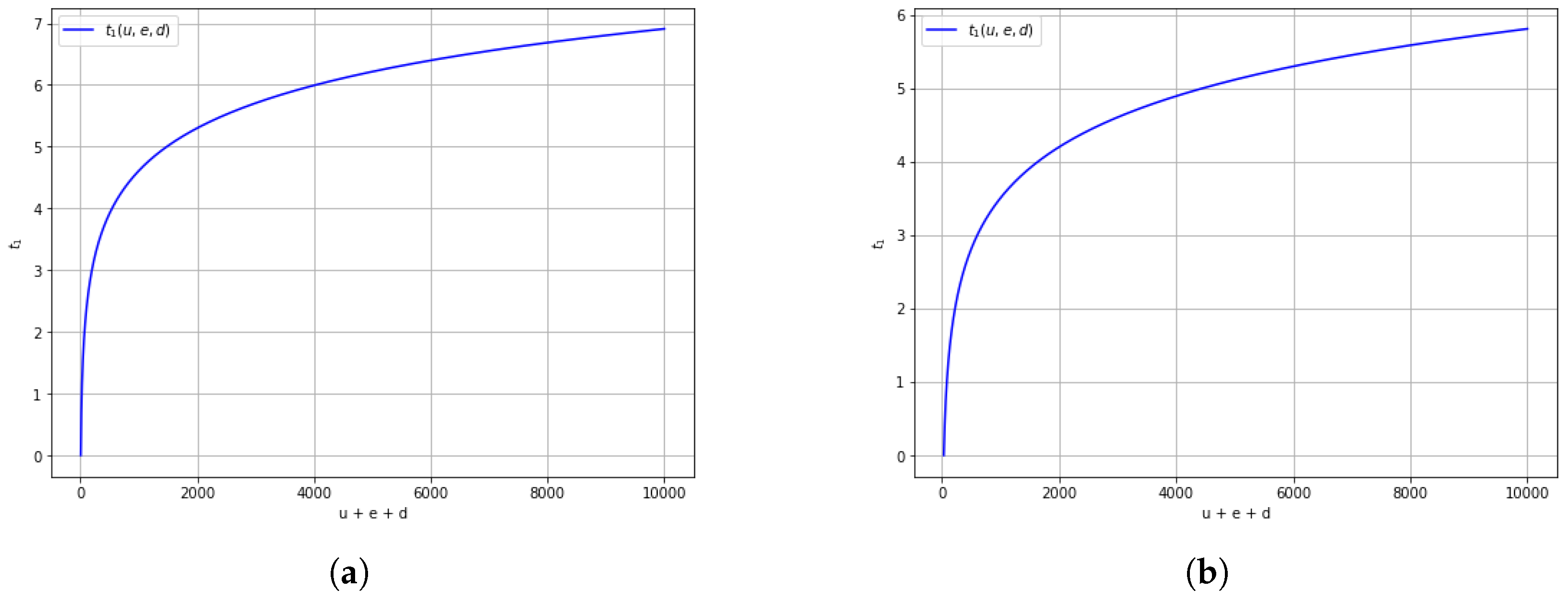
Figure 5a,b illustrate how the recovery time $t_1$ varies with the total initial condition $u+e+d$ and with different values of the regulatory threshold $\lambda$, at a fixed recovery rate $\gamma =1$. As the initial burden of distress increases, so does $t_1$, indicating longer periods before recovery begins. Notably, a higher threshold $\lambda$ (Figure 5b) leads to earlier exit from the critical distress zone, even if full recovery is not yet achieved. These figures reinforce how threshold selection affects the perceived timing of systemic recovery.

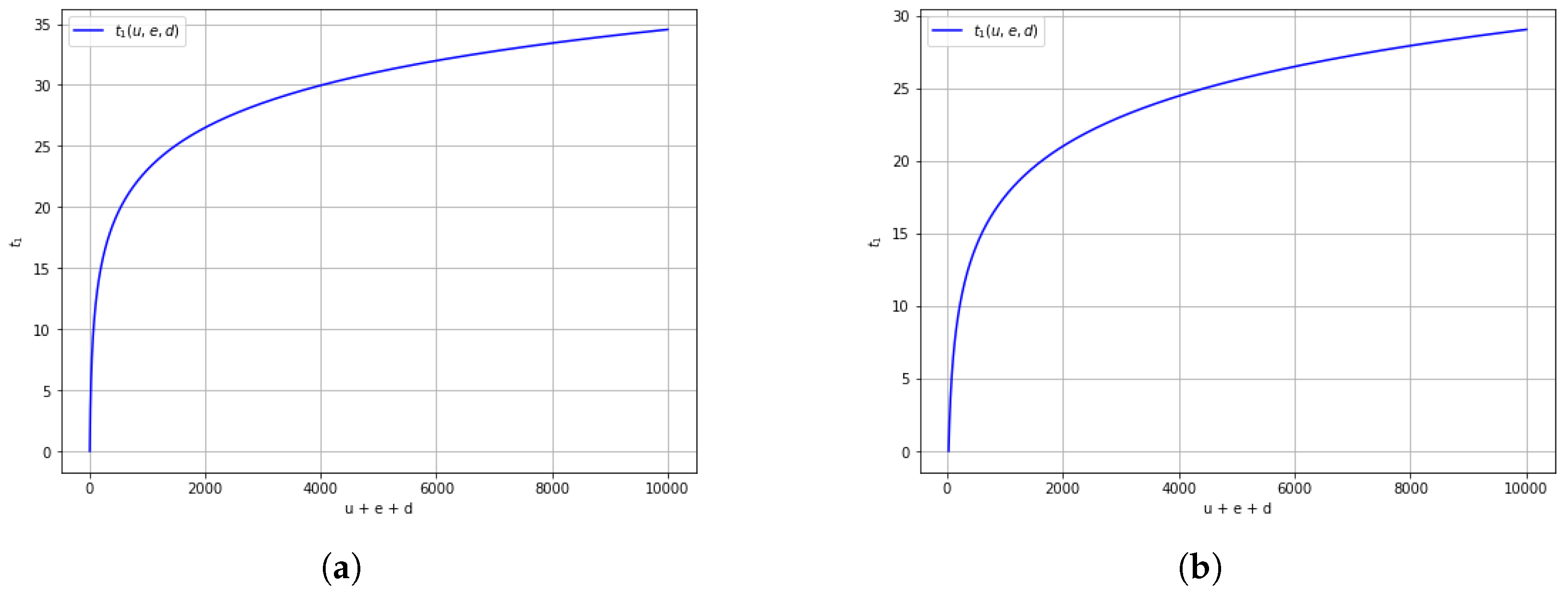
Figure 6a,b explore the effect of a lower recovery rate ($\gamma =0.2$) on $t_1$ under the same range of $u+e+d$. Compared to the previous figures, $t_1$ is consistently higher, emphasizing that slower recovery mechanisms delay containment of systemic distress. These results highlight the critical role of regulatory support and recapitalization speed in shaping recovery timelines.

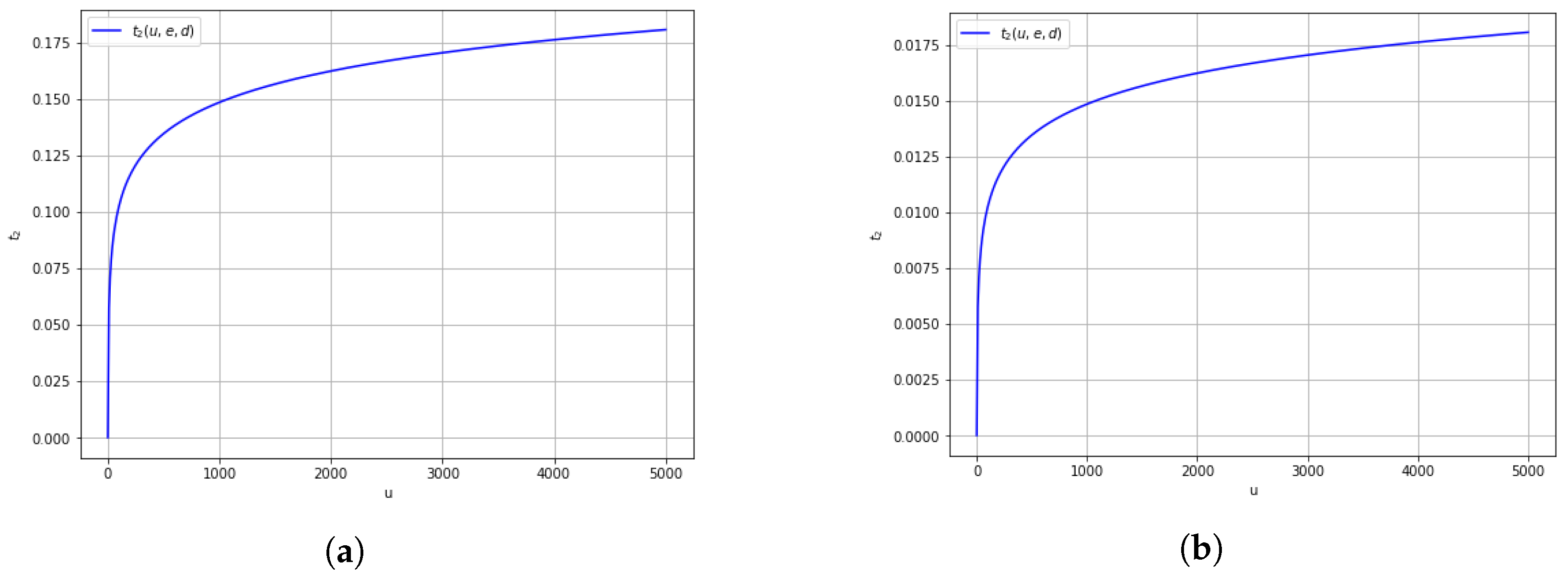
Figure 7a,b display the transition time $t_2$ as a function of undistressed banks u when recovery and transmission rates are equal ($\gamma =\beta$) for two levels of distressed banks ($d=10$ and $d=100$). A higher initial number of distressed banks leads to a significantly earlier onset of instability (lower $t_2$), even when initial conditions seem stable. These figures demonstrate how latent stress levels shorten the safe window for policy response.

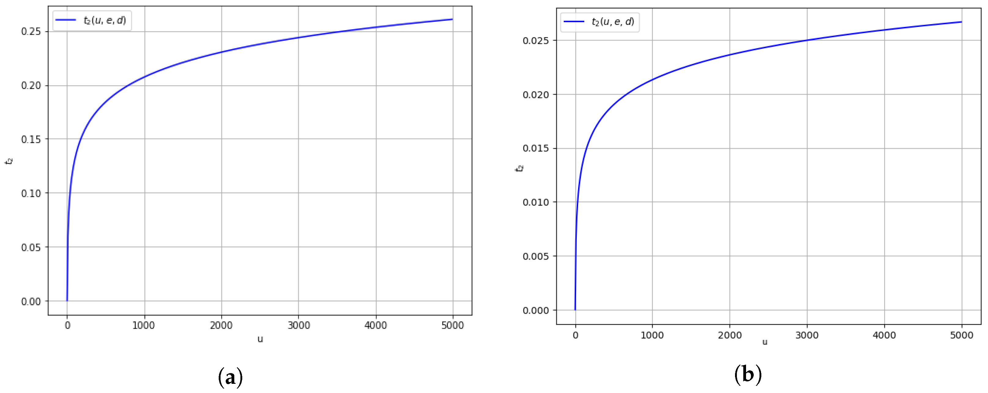
Figure 8a,b consider the case where contagion outpaces recovery ($\gamma <\beta$). The results show a rapid decrease in $t_2$ as u declines, especially when d is large. This configuration reflects a highly fragile system where systemic stability can be lost quickly. Such scenarios call for proactive monitoring and early policy intervention to prevent sudden collapses.

Figure 9a,b reflect the behavior of $t_2$ in systems with strong recovery capacity ($\gamma >\beta$). Here, even in the presence of high distress levels, the system remains resilient longer, and $t_2$ increases steadily with u. These results underscore the effectiveness of enhancing recovery mechanisms—such as capital surcharges and emergency funding—in delaying systemic breakdowns.

Comparing Figure 7a to Figure 9b, we observe that as the recovery rate approaches or exceeds the distress transmission rate, the significance of the first instance when undistressed banks fall below a specific threshold becomes more pronounced. This observation aligns with the concept that when the distressed banks recover substantially (i.e., when $\gamma >\beta$), the undistressed banks do not diminish at the same rate as when the distressed banks recover slowly (when $\gamma <\beta$). Furthermore, we notice an inverse relationship between the increase in distressed banks and the initial time when the number of undistressed banks falls below a certain threshold. This implies that a higher increase in distressed banks leads to a quicker occurrence of the number of undistressed banks falling below the specified threshold.

The numerical findings in this section support and extend prior studies on financial contagion dynamics. In particular, while Mourad et al. [3] and Chen and Fan [4] investigated contagion using SIR-type models, their analyses focused primarily on long-term equilibria or peak distress levels. By contrast, this study quantifies the timing of contagion containment ($t_1$) and the onset of systemic risk recovery ($t_2$), offering time-sensitive indicators for real-time policy intervention. For example, simulations in Figure 5 and Figure 6 show that when $\gamma =1$, $\lambda =10$, and the total number of banks $u+e+d=20$, the time to risk containment $t_1$ is approximately 2.8. However, when $\gamma$ is reduced to 0.2 under the same initial conditions, $t_1$ rises significantly to approximately 8.3, indicating a delayed recovery due to slower response mechanisms. Similarly, Figure 7, Figure 8 and Figure 9 show that for $\beta =\gamma =3$ and initial distressed banks $d=100$, the onset of instability $t_2$ occurs within the first 0.5 units of time when $u=5$. This sharp contraction in $t_2$ under high stress levels is not directly captured in traditional SIR-based models but is clearly delineated in the UEDR framework. These results provide concrete thresholds—such as $U\left(t\right)\le \gamma /\beta$ and $D\left(t\right)\le \lambda$—that are not only mathematically justified but also practically aligned with supervisory tolerance levels. Thus, the model contributes a temporal dimension to systemic risk analysis, bridging a key gap in the literature and equipping regulators with tools for anticipatory action. Unlike Irakoze et al. [5], who emphasized model formulation and stability analysis, we provide concrete numerical thresholds and visualizations that connect directly to regulatory decision-making. For instance, when $\gamma =1$, $\lambda =10$, and the total number of banks is $u+e+d=20$, simulations in Figure 5 and Figure 6 show that the time to containment ($t_1$) is approximately 2.8. When the recovery rate is reduced to $\gamma =0.2$ under the same conditions, $t_1$ increases to around 8.3, indicating delayed recovery. Similarly, as shown in Figure 7, Figure 8 and Figure 9, when $d=100$ and $u=5$, the time to fragility ($t_2$) falls below 0.5, highlighting rapid loss of resilience under extreme stress. These outcomes—anchored in thresholds such as $U\left(t\right)\le \gamma /\beta$ and $D\left(t\right)\le \lambda$—offer regulators actionable benchmarks for stress testing and intervention planning. As such, this work adds a temporal, predictive layer to the static and qualitative insights of previous UEDR-based studies. The numerical findings in this section build on and extend prior studies on systemic risk dynamics.

7. Conclusions and Recommendation

This study provides a rigorous analytical framework for understanding the time dynamics of systemic risk in banking networks, using a compartmental UEDR (Undistressed–Exposed–Distressed–Recovered) model. By introducing and characterizing two critical time indicators—$t_1$, the point at which the number of distressed banks falls below a regulatory threshold, and $t_2$, the point when undistressed banks fall below a resilience threshold—we offer a dynamic approach to quantifying financial stability and fragility. The explicit representation, continuity, and asymptotic behavior of these time functions yield key insights for systemic risk monitoring. In particular, our findings show that $t_1$ grows with the severity of initial distress, while $t_2$ contracts, indicating a narrowing window for effective intervention. These results equip policymakers and regulators with tools to better anticipate and respond to systemic crises.

Practically, this framework can inform the design of time-sensitive regulatory thresholds, such as trigger points for emergency liquidity provision, capital buffer adjustments, or macroprudential interventions. The integration of these transition times into stress testing and early-warning systems enhances the ability to detect tipping points and allocate regulatory resources more efficiently. Overall, this research contributes a novel and actionable lens for managing systemic risk in interconnected financial systems.