Mathematical Perspectives on Consumer Spending during a Financial Crisis

Abstract

This paper explores the mathematical dynamics of consumer spending during a financial crisis using opponent process theory (OPT). Traditionally applied in psychology, OPT explains how initial emotional responses are followed by counteracting reactions to restore equilibrium. This study models the short-term boost in consumer spending and subsequent economic adjustments. Utilizing differential equations to represent these processes, this paper provides insights into the interplay between immediate policy effects and longer-term economic consequences. We focus on the United States (US) response to the 2008 Global Financial Crisis in this study. Results show evidence of diminishing response from prolonged stimuli due to demand saturation, resource allocation inefficiencies, and agent adaptation. Monetary stimuli may inflate debt/prices, outweighing benefits, and structural issues persist despite stimuli. Confidence and expectations impact response because perceived ineffectiveness weakens impact over time. Thus, while stimuli can initially boost activity, their sustained impact demands careful consideration of economic dynamics and agents’ responses.

1. Introduction

The Global Financial Crisis (GFC) of 2008 stands as one of the most significant economic upheavals of the 21st century, sending shockwaves through financial systems and economies worldwide [1,2]. Triggered by the collapse of Lehman Brothers and the ensuing meltdown in the housing market, the crisis exposed the vulnerabilities within the global financial architecture. It led to unprecedented fiscal and monetary interventions aimed at stabilizing economies and restoring confidence [3,4]. The crisis also provided fertile ground for the application of various economic theories and models to understand the dynamics of consumer behavior and economic recovery.

One such theoretical framework that can be applied to understand the economic dynamics during the GFC is opponent process theory (OPT) [5,6], originally developed in the context of psychology to explain emotional responses. OPT posits that every emotional experience is followed by a contrasting counter-response, aiming to restore equilibrium (also see [7]). When adapted to economics, particularly to consumer spending behavior, this theory sheds light on how initial stimuli, such as government interventions, can induce immediate positive effects followed by subsequent negative adjustments. By applying OPT to the GFC, we aim to provide unique insights into the interplay between initial government interventions and their long-term economic effects, allowing for a deeper understanding of consumer behavior during the crisis. The approach uniquely clarifies consumer behavior during the financial crisis by modeling the immediate positive effects of government interventions and subsequent negative adjustments.

The socio-economic impacts of the GFC were extensive and far-reaching, affecting not only financial markets but also the broader societal fabric. One of the significant consequences was the exacerbation of income inequality [8,9]. As financial markets collapsed and unemployment soared, wealth disparities widened, with lower-income individuals and families bearing the brunt of the economic downturn [10]. High-income earners and those with substantial financial assets were able to recover more swiftly, while the middle and lower classes faced prolonged economic hardship. This divergence has had lasting effects on social cohesion and economic mobility. Additionally, the GFC induced significant shifts in migration patterns. The economic uncertainty and job losses prompted many individuals to migrate in search of better opportunities. This trend was evident both within countries, as people moved from economically distressed regions to more stable areas, and internationally, as migrants sought employment in countries less affected by the crisis [11]. Such migration flows have had complex implications for labor markets, social services, and political dynamics in both origin and destination regions.

During the GFC, governments worldwide deployed substantial fiscal stimuli and bailout packages to prevent the complete collapse of financial systems. For instance, the U.S. government passed the Emergency Economic Stabilization Act in 2008, which included the Troubled Asset Relief Program (TARP) [12,13]. These interventions can be analogized to an initial dopamine response in the brain [14,15], triggering a surge in consumer confidence and spending. However, the effectiveness of such stimuli has been debated, particularly regarding their long-term sustainability and the balance between immediate relief and long-term economic stability. As per the OPT, this initial surge (analogous to the a-process) would be followed by a b-process, where the negative consequences of increased debt and economic adjustment processes begin to manifest. Studies have shown that the marginal impact of fiscal and monetary stimuli tends to diminish over time due to factors like demand saturation and resource allocation inefficiencies [16].

Empirical research has documented the phenomenon of consumer habituation, where the impact of a stimulus (e.g., tax cuts, cash transfers) on consumption tends to decay over time as consumers adapt [17,18]. This adaptation process highlights the importance of evaluating not just the immediate effects of fiscal policies but also their longer-term implications on consumer behavior and economic health. Researchers have developed models that capture the dynamic relationship between stimulus and consumption, often incorporating exponential decay functions [19,20]. In addition, some studies have emphasized the importance of considering the temporal dynamics and sustained effectiveness of stimulus policies when designing and evaluating economic interventions [16,21]. Our approach builds on these models by explicitly incorporating the OPT framework to provide a more nuanced understanding of the interplay between immediate and long-term effects.

To illustrate the dynamics of the efficacy of a stimulus, we employ a deterministic model capturing the rise and fall (or persistence) of economic activity in response to stimuli. This model involves time-dependent variables representing the immediate economic boost and the subsequent decay over time, similar to how dopamine activity exhibits an exponential decay after an initial spike. By incorporating both immediate and delayed effects, our model provides a comprehensive view of how fiscal stimuli influence economic activity over different time horizons. Through modeling consumer spending in response to the fiscal stimuli during the GFC, we can better understand the short-term gains and the longer-term economic adjustments that followed. The a-process in this economic analogy represents an initial increase in consumer spending and economic activity, spurred by the stimulus. We model this concept using differential equations that capture the rise in spending due to the injected liquidity. However, as the effects of the stimulus wane, the b-process kicks in, representing the reduction in spending and the negative effects, such as increased household debt and reduced savings, which we also model using differential equations, capturing the gradual decline in the initial positive impact. This dual-process modeling approach allows us to identify potential tipping points where the benefits of stimulus measures may be outweighed by their longer-term costs.

The outward dynamics observed during or immediately after a financial crisis are primarily because of consumer behaviour. A study in [22] shows that consumers become more selective and concentrate their spending only on what they consider necessary for survival. They become more aware of prices, avoid impulsive purchases, and adopt a more cautious, saving-oriented approach to their finances according to [23]. As an extension of the investigation of the effects of the GFC, the author in [24] aims to evaluate and compare different methods for estimating fiscal multipliers, revealing that most estimates fall within specific ranges, to measure economic growth, which is primarily driven by consumption dynamics. A study in [25] focused on the COVID-19-driven financial crisis. This article aims to examine how fiscal policy has changed due to the COVID-19 pandemic and how it might evolve in the post-COVID era, in which they viewed the economic dynamics as a return to the Keynesian economics.

Our contribution in this work is defined by the fact that, by applying the opponent process model to the GFC, we obtain insights into the interplay between immediate policy effects and longer-term economic adjustments. This approach not only enhances our understanding of the crisis but can also inform the design of future economic policies, ensuring they are balanced to maximize short-term benefits while mitigating long-term negative consequences. By integrating recent advancements in economic modeling with the OPT framework, we offer a refined perspective on the effectiveness of fiscal stimuli. Through this perspective, we show that while stimulus measures can provide short-term support to the economy during downturns, their long-term effectiveness depends on various factors. There may be diminishing returns or unintended consequences associated with continued stimulation, such as distorted market signals, inflationary pressures, and asset bubbles ,among others. Hence, it is essential for policymakers to carefully assess the economic context and the potential risks and benefits of continued stimulating. This approach highlights the need for adaptive policy strategies that evolve based on empirical evidence and changing economic conditions.

The paper is arranged as follows: In Section 1, we present the introduction. This is followed by model formulation in Section 2. In Section 3, we give the results of the mathematical model, followed by the discussion and conclusion in Section 4.

2. Model Formulation and Analysis

We formulate a mathematical model that describes the consumer spending dynamics during a financial crisis. We show that the solutions from the model system are bounded, and are always positive. We further explore the stability of the system and extract results from the model to show the effectiveness of the model.

2.1. The Model

To model the dynamics of consumer spending in response to economic stimuli, we use the logistic growth function to effectively capture the rapid initial increase in consumption that slows down as it approaches a saturation point, reflecting the natural limits of consumption growth. The logistic function is characterized by three key parameters: the initial level of consumption ($C_0$), the intrinsic growth rate (r), and the carrying capacity (k), which represents the maximum sustainable level of consumption. The logistic differential equation describes how consumption changes over time, with the growth rate slowing as consumption nears its carrying capacity. Setting $C\left(t\right)$ as the level of consumption at time t, r as the intrinsic growth rate, and k as the carrying capacity, the logistic growth equation for consumption is given by the following:

$${\displaystyle \frac{dC}{dt}}=rC\left(1-{\displaystyle \frac{C}{k}}\right)C\left(0\right)=C_0.$$

(1)

All parameters are assumed to be non-negative. The solution to this differential equation, which describes the time-dependent behavior of consumption, is as follows:

$$C\left(t\right)={\displaystyle \frac{k}{1+\left(\frac{k-C_0}{C_0}\right)e^{-rt}}}$$

(2)

This function effectively models the initial surge in consumer spending in response to an economic stimulus, the slowing of growth as consumption approaches the carrying capacity, and the eventual stabilization of consumption levels. The initial impact of significant stimulus packages and bailouts can be likened to an a-process ${\sigma }_a\left(t\right)$, representing the initial increase in consumer spending and economic activity. We let $\alpha$ represent the intrinsic decay rate of the a-process; ${\mathsf{\Omega }}_a$ reflects the coupling of the stimulus to the increase in spending. This surge in spending is analogous to the pleasurable a-process triggered by the stimulus. To model this, we utilize the following equation:

$${\displaystyle \frac{d{\sigma }_a\left(t\right)}{dt}}=-\alpha {\sigma }_a\left(t\right)+{\mathsf{\Omega }}_{a}C\left(t\right),{\sigma }_a\left(0\right)\ge 0.$$

(3)

We assume that all parameters are non-negative. The subsequent reduction in spending and negative effects can be likened to a b-process ${\sigma }_b\left(t\right)$. As the initial stimulus wanes, the economy may experience negative consequences such as increased debt levels, reduced savings, and eventual economic contraction. We set $\beta$ to represent the intrinsic decay rate of the b-process, and ${\mathsf{\Omega }}_b$ to denote the coupling of the a-process to the b-process. This mirrors the unpleasant b-process activated as a counteracting response to the stimulus. and the parameter $\gamma$ determines the strength of this coupling. We model this with the following equation:

$${\displaystyle \frac{d{\sigma }_b\left(t\right)}{dt}}=-\beta {\sigma }_b\left(t\right)-(1-\gamma ){\mathsf{\Omega }}_b{\sigma }_a\left(t\right),{\sigma }_b\left(0\right)\ge 0.$$

(4)

where we assume all the model parameters to be non-negative. Then, we obtain the model system:

$$\begin{array}{c}{\displaystyle \frac{d{\sigma }_a\left(t\right)}{dt}}=-\alpha {\sigma }_a\left(t\right)+{\mathsf{\Omega }}_{a}C\left(t\right),\hfill \\ {\displaystyle \frac{d{\sigma }_b\left(t\right)}{dt}}=-\beta {\sigma }_b\left(t\right)-(1-\gamma ){\mathsf{\Omega }}_b{\sigma }_a\left(t\right).\hfill \end{array}$$

(5)

2.2. Model Analysis

Before we proceed with our critical analysis of the model system (5), we show that the system has positive bounded solutions, and reflect on the stability of its equilibrium points. While this may seem trivial from the solutions to the model system, we provide Theorems 1 and 2, which reinforce this claim.

Theorem 1 (Positivity).

Consider the system of differential equations,

$$\begin{array}{cc}\hfill {\displaystyle \frac{d{\sigma }_a\left(t\right)}{dt}}& =-\alpha {\sigma }_a\left(t\right)+{\mathsf{\Omega }}_{a}C\left(t\right),\hfill \\ \hfill {\displaystyle \frac{d{\sigma }_b\left(t\right)}{dt}}& =-\beta {\sigma }_b\left(t\right)-(1-\gamma ){\mathsf{\Omega }}_b{\sigma }_a\left(t\right),\hfill \end{array}$$

with positive parameters $\alpha ,\beta ,{\mathsf{\Omega }}_a,{\mathsf{\Omega }}_b>0$ and positive initial values ${\sigma }_a\left(0\right)>0$ and ${\sigma }_b\left(0\right)>0$. Assume $C\left(t\right)\ge 0$ and $\gamma \ge 1$ for all $t\ge 0$. Then, the solutions ${\sigma }_a\left(t\right)$ and ${\sigma }_b\left(t\right)$ remain positive for all $t\ge 0$.

Proof. 

First, consider the equation for ${\sigma }_a\left(t\right)$:

$${\displaystyle \frac{d{\sigma }_a\left(t\right)}{dt}}=-\alpha {\sigma }_a\left(t\right)+{\mathsf{\Omega }}_{a}C\left(t\right).$$

This is a linear first-order differential equation with the following general solution:

$${\sigma }_a\left(t\right)=e^{-\alpha t}\left({\sigma }_a\left(0\right)+{\int }_0^t{\mathsf{\Omega }}_{a}C\left(s\right)e^{\alpha s}ds\right).$$

Given that ${\sigma }_a\left(0\right)>0$, $\alpha >0$, ${\mathsf{\Omega }}_a>0$, and $C\left(t\right)\ge 0$ for all $t\ge 0$, the term $e^{-\alpha t}$ is always positive, and the integral term is non-negative. Therefore, ${\sigma }_a\left(t\right)>0$ for all $t\ge 0$.

Consider the equation for ${\sigma }_b\left(t\right)$:

$${\displaystyle \frac{d{\sigma }_b\left(t\right)}{dt}}=-\beta {\sigma }_b\left(t\right)-(1-\gamma ){\mathsf{\Omega }}_b{\sigma }_a\left(t\right).$$

This is also a linear first-order differential equation with the following general solution:

$${\sigma }_b\left(t\right)=e^{-\beta t}\left({\sigma }_b\left(0\right)-{\int }_0^t(1-\gamma ){\mathsf{\Omega }}_b{\sigma }_a\left(s\right)e^{\beta s}ds\right).$$

Given that ${\sigma }_b\left(0\right)>0$, $\beta >0$, ${\mathsf{\Omega }}_b>0$, and $\gamma >0$, since we have already shown that ${\sigma }_a\left(t\right)>0$ for all $t\ge 0$, the term $e^{-\beta t}$ is always positive, and the integral term is non-positive. Therefore, ${\sigma }_b\left(t\right)$ remains positive for all $t\ge 0$ provided that $\gamma \ge 1$. □

Theorem 2 (Boundedness of solutions).

Consider the system of differential equations,

$$\begin{array}{cc}\hfill {\displaystyle \frac{d{\sigma }_a\left(t\right)}{dt}}& =-\alpha {\sigma }_a\left(t\right)+{\mathsf{\Omega }}_{a}C\left(t\right),\hfill \\ \hfill {\displaystyle \frac{d{\sigma }_b\left(t\right)}{dt}}& =-\beta {\sigma }_b\left(t\right)-(1-\gamma ){\mathsf{\Omega }}_b{\sigma }_a\left(t\right),\hfill \end{array}$$

with positive parameters $\alpha ,\beta ,{\mathsf{\Omega }}_a,{\mathsf{\Omega }}_b>0$ and positive initial values ${\sigma }_a\left(0\right)>0$ and ${\sigma }_b\left(0\right)>0$. Assume $C\left(t\right)$ is bounded for all $t\ge 0$. Then, the solutions ${\sigma }_a\left(t\right)$ and ${\sigma }_b\left(t\right)$ are bounded for all $t\ge 0$.

Proof. 

Given that $C\left(t\right)>0$, the proof follows trivially from the explicit formulas for ${\sigma }_a\left(t\right)$ and ${\sigma }_b\left(t\right)$. □

2.3. Stability Analysis

The given system (5) has the solution

$$\begin{array}{cc}\hfill {\sigma }_a\left(t\right)& ={\displaystyle \frac{C_{0}k{\mathsf{\Omega }}_a{e}^{rt}}{\alpha \left(C_0{e}^{rt}-C_0+k\right)}},\hfill \\ \hfill {\sigma }_b\left(t\right)& ={\displaystyle \frac{C_0(\gamma -1)k{\mathsf{\Omega }}_a{\mathsf{\Omega }}_b{e}^{rt}}{\alpha \beta \left(C_0{e}^{rt}-C_0+k\right)}}.\hfill \end{array}$$

The steady state $({\sigma }_a,{\sigma }_b)$ exists if $\gamma \ge 1$.

The model system has the Jacobian matrix:

$$J=\left(\begin{array}{cc}-\alpha & 0\\ -(1-\gamma ){\mathsf{\Omega }}_b& -\beta \end{array}\right)$$

(6)

Since the Jacobian matrix, J, is lower-triangular, its eigenvalues are simply the diagonal entries. Therefore, the eigenvalues of J are $-\alpha$ and $-\beta$. The eigenvalues $-\alpha$ and $-\beta$ both have negative real parts. This indicates that the equilibrium point is stable, that small perturbations around the equilibrium point will decay over time, and that the system will return to the equilibrium point.

3. Results and Simulations

Defining a parameter, $\varphi$, which represents the various factors influencing the consumption experience, such as the initial level of consumption, intrinsic growth rates, and coupling strengths, between the different processes, we obtain the overall impact of consumption dynamics over time:

$$\sigma \left(t\right|\varphi )={\sigma }_a\left(t\right)+{\sigma }_b\left(t\right),$$

(7)

where $\varphi =\{r,\alpha ,\beta ,{\mathsf{\Omega }}_a$,${\mathsf{\Omega }}_b\}$. Consequently, from (7), given $({\sigma }_a,{\sigma }_b)$, we have the following:

$$\sigma \left(t\right|\varphi )={\displaystyle \frac{C_{0}k{\mathsf{\Omega }}_a{e}^{rt}\left((\gamma -1){\mathsf{\Omega }}_b+\beta \right)}{\alpha \beta \left(C_0\left(e^{rt}-1\right)+k\right)}}.$$

(8)

Result 1.

Economic stimulus leads to an increase in consumption over time.

Proof. 

The cumulative impact of past consumption experiences on future decision-making regarding spending behaviors, ${\kappa }_p$, is given by the integral of $\sigma \left(t\right|\varphi )$ in the time domain, $(0,\infty )$, to obtain the following:

$${\kappa }_p={\int }_0^{\infty }\sigma \left(t\right|\varphi )dt={\displaystyle \frac{{\mathsf{\Omega }}_{a}klog(k-C_0+C_0{e}^{rt})(\beta -{\mathsf{\Omega }}_b+{\mathsf{\Omega }}_b\gamma )}{\alpha \beta r}}$$

(9)

This is a monotonically increasing function, showing growth over time, which is consistent with the Multiplier Effect, Endogenous Growth Theory and the Permanent Income Hypothesis and Life-Cycle Hypothesis. □

The integral involves the logarithmic term $log(k-C_0+C_0{e}^{rt})$, capturing the cumulative effect of consumption dynamics relative to initial conditions and growth rate. As time t increases, $e^{rt}$ grows exponentially, influencing the balance between initial consumption and exponential growth driven by rate r. For a large t value, the term $C_0{e}^{rt}$ dominates, making the logarithmic term significant, indicating cumulative effect growth over time influenced by intrinsic rate r and initial conditions.

The total economic impact of the cumulative effect of successive economic policies or stimuli over time would be a superposition of the individual impacts of each policy measure, with each having its parameters that determine its effectiveness and decay over time. The successive responses to economic stimuli are given by the following:

$$\sigma (t\mid \{{\varphi }_i\le k\})=\sum _{i=1}^k\sigma (t-T_i\mid {\varphi }_i),$$

(10)

where $T_1\equiv 0$, $T_k<t<T_{k+1}$, and ${\varphi }_i=\{C_{0i},r_i,k_i,{\alpha }_i,{\mathsf{\Omega }}_{ai},{\beta }_i,{\mathsf{\Omega }}_{bi}\}$ are the parameters of the system following the i-th economic stimulus.

The total response $\sigma (t\mid \{{\varphi }_i\le k\})$ is the sum of individual responses, $\sigma (t-T_i\mid {\varphi }_i)$. Each response is shifted in time by $T_i$, representing the time at which each economic stimulus occurs. The parameters ${\varphi }_i$ define the characteristics of each stimulus. Specifically, $C_{0i}$ is the initial level of consumption after the i-th stimulus, $r_i$ is the intrinsic growth rate of consumption for the i-th stimulus, $k_i$ is the carrying capacity or maximum sustainable level of consumption for the i-th stimulus, ${\alpha }_i$ is the decay rate of the a-process for the i-th stimulus, ${\mathsf{\Omega }}_{ai}$ reflects the coupling of the stimulus to the increase in consumption for the i-th stimulus, ${\beta }_i$ is the decay rate of the b-process for the i-th stimulus, and ${\mathsf{\Omega }}_{bi}$ denotes the coupling strength between the a-process and the b-process for the i-th stimulus.

The combined response function, given the individual response function for each stimulus, is as follows:

$$\sigma (t\mid {\varphi }_i)={\displaystyle \frac{C_{0i}{k}_i{\mathsf{\Omega }}_{ai}{e}^{r_{i}t}({\beta }_i-{\mathsf{\Omega }}_{bi})}{{\alpha }_i{\beta }_i(C_{0i}(e^{r_{i}t}-1)+k_i)}}.$$

(11)

Result 2.

Intertemporal dynamics of stimulus-driven consumption changes diminish relative to the consumption decay factor and to consumption efficiency.

Proof. 

The limit of $\sigma \left(t\right|{\varphi }_i)$ as t approaches infinity is given by the following:

$${\displaystyle \underset{t\to \infty }{lim}\sigma (t\mid {\varphi }_i)=\left\{\begin{array}{cc}0,\hfill & \mathrm{if}{\mathsf{\Omega }}_{b_i}={\beta }_i\mathrm{or}{C}_{0_i}=0\mathrm{or}{\mathsf{\Omega }}_{a_i}=0\mathrm{or}{k}_i=0\hfill \\ {\displaystyle -\underset{t\to \infty }{lim}\frac{C_{0_i}{\mathsf{\Omega }}_{a_i}{k}_i{e}^{r_{i}t}({\mathsf{\Omega }}_{b_i}-{\beta }_i)}{k_i+C_{0_i}(e^{r_{i}t}-1)},}\hfill & \mathrm{otherwise}.\hfill \end{array}\right.}$$

(12)

Now,

$${\displaystyle -\underset{t\to \infty }{lim}\frac{C_{0_i}{\mathsf{\Omega }}_{a_i}{k}_i{e}^{r_{i}t}({\mathsf{\Omega }}_{b_i}-{\beta }_i)}{k_i+C_{0_i}(e^{r_{i}t}-1)}=\frac{C_{0_i}{\mathsf{\Omega }}_{a_i}({\beta }_i-{\mathsf{\Omega }}_{b_i})}{{\alpha }_i{\beta }_i},}$$

which is simply the quotient of stimulus-driven consumption change divided by the consumption decay factor, that is, the consumption efficiency. Hence, in the long run, the successive responses to economic stimuli converge into consumption efficiency. □

The total time-dependent response to successive economic stimuli is then given by the following:

$$\sigma (t\mid \{{\varphi }_i\le k\})=\sum _{i=1}^k{\displaystyle \frac{C_{0i}{k}_i{\mathsf{\Omega }}_{ai}{e}^{r_i(t-T_i)}({\beta }_i-{\mathsf{\Omega }}_{bi})}{{\alpha }_i{\beta }_i(C_{0i}(e^{r_i(t-T_i)}-1)+k_i)}},$$

(13)

where $T_1\equiv 0$, $T_k<t<T_{k+1}$.

Simulations Using the US Consumption Data from 2000–2022

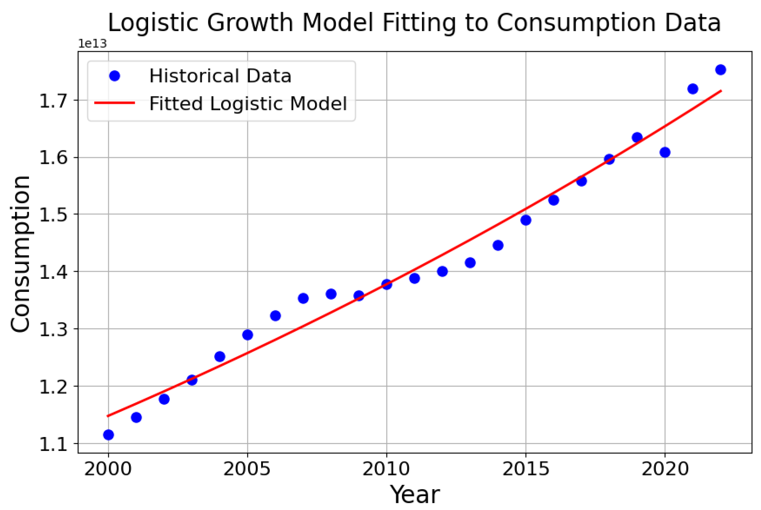
To simulate the results from this work, we consider using consumption data from a developed country such as the United States of America (US). These data by themselves give the key economic indicators of parameters such as the carrying capacity, and can be manipulated to estimate the intrinsic growth rate and the initial consumption levels. The rationale is that the data are reliable, and the government’s response to the 2008 Global Financial Crisis is well documented. We used data from the World Bank database, which are available publicly. To calibrate the logistic growth model using historical consumption data, we prepare the data into a time-series format, making initial guesses for the model parameters $C_0$, r, and k, and then use optimization techniques to fit the model and estimate the optimal parameter values. We then assess the goodness-of-fit and statistical significance of the calibrated model, interpret the estimated parameters, conduct sensitivity analysis, refine the model as needed, and validate it with out-of-sample data. We start by fitting the data to $C\left(t\right)$ as shown in Figure 1.

The high coefficient of determination ($R^2$=0.974) indicates that the fitted model explains roughly 97.4% of the variation in the observed consumption data, suggesting a strong fit between the model predictions and actual consumption trends.

We obtain the table of parameters in

Table 1. Summary of parameters.

Parameter	Description	Value
$C_0$	Estimated initial consumption level	$1.147\times {10}^{13}$
r	Estimated intrinsic growth rate	0.0183
K	Estimated maximum sustainable consumption level	$2.717\times {10}^{19}$
$\alpha$	The intrinsic decay rate of ${\sigma }_a\left(t\right)$	0.5048
$\beta$	The intrinsic decay rate of the b-process	0.4952
${\mathsf{\Omega }}_a$	The coupling of the stimulus to the increase in spending	0.2225
${\mathsf{\Omega }}_b$	The coupling of the a-process to the b-process	0.2146
$\gamma$	The strength of coupling of the a-process to the b-process	1.3

from the fit. in Figure 1

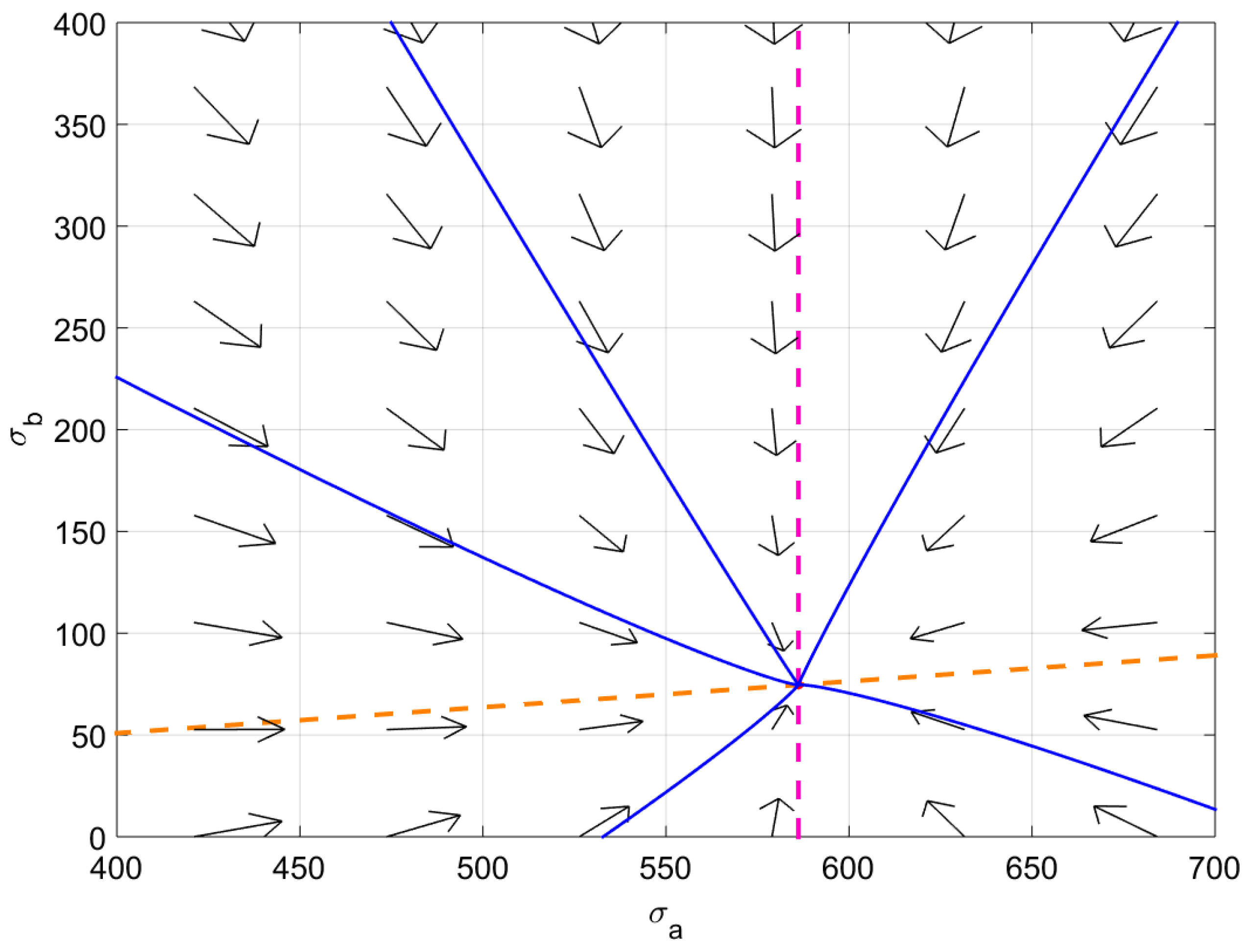
All the times used for the simulations are presented in days. Using the parameter values in Table 1, we have the following phase plane in Figure 2 that shows that the model system converges to a locally stable steady state, $E=\left(586.75\right)$.:

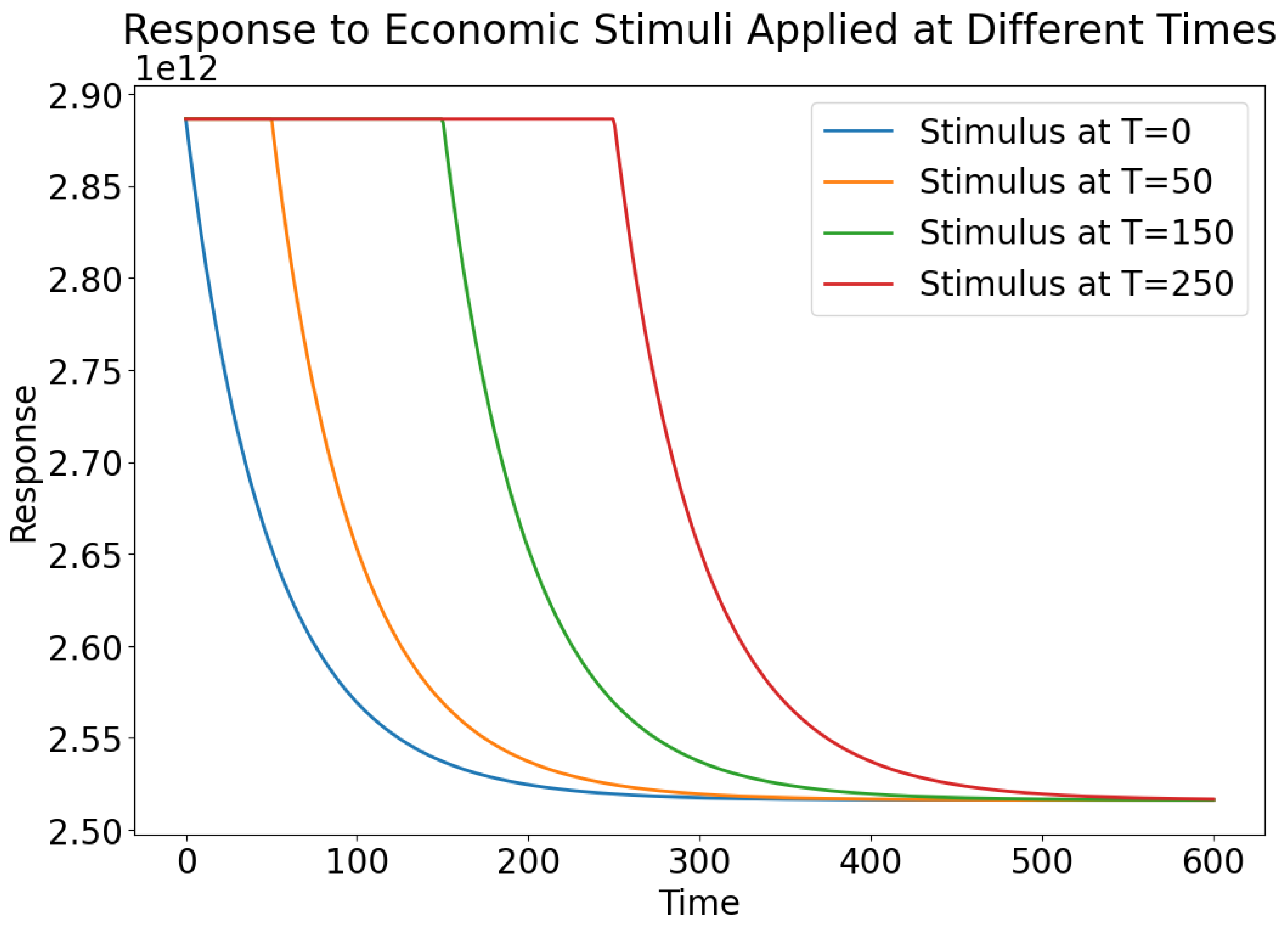
From Result 2, we demonstrate in Figure 3 that introducing stimuli at various time points is effective, but the consumption behaviour in each instance similarly converges to the consumption efficiency.

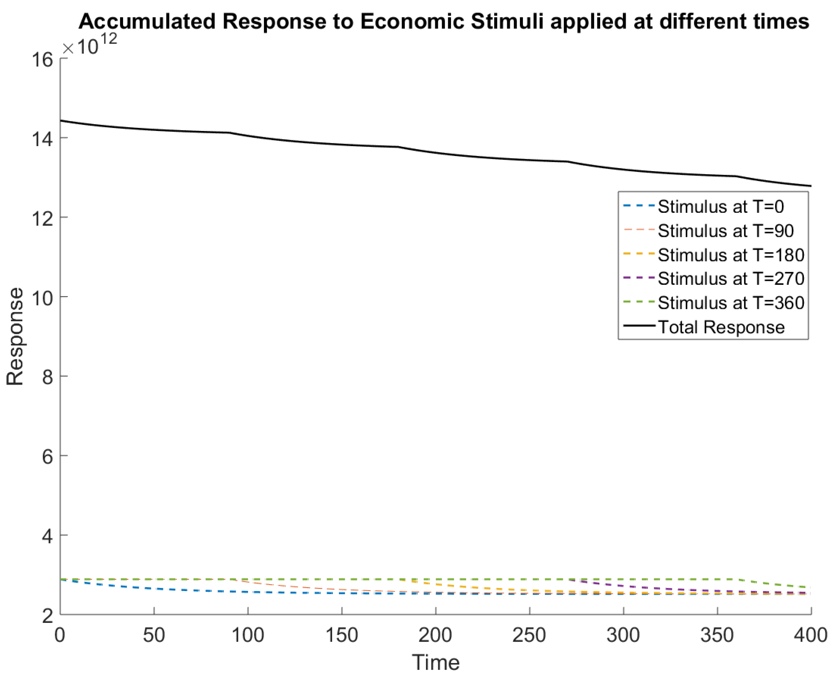
Despite the accumulation of both fading and newly introduced stimuli, total consumption gravitates towards a convergent point. This phenomenon underscores the dynamic equilibrium achieved within the economic system, where the combined effects of stimuli gradually stabilize over time. Figure 4 illustrates the convergence of total consumption towards a steady state, even in the presence of overlapping multiple stimuli.

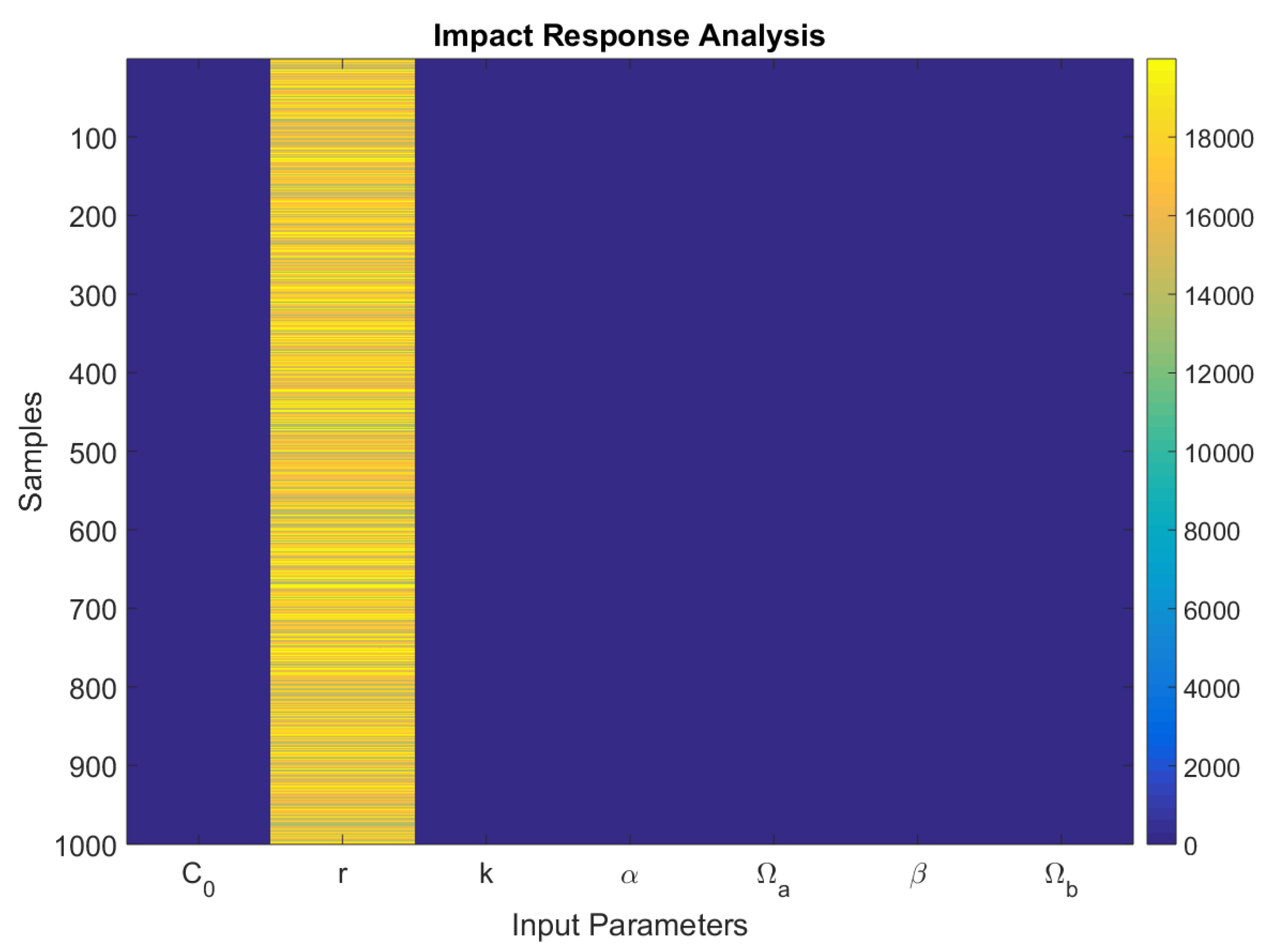
The most influential input parameter appears to be the growth rate, r, as indicated by the large impact response values in the second column of the output. This means that small changes in the growth rates significantly impact the model outputs. This is demonstrated in Figure 5.

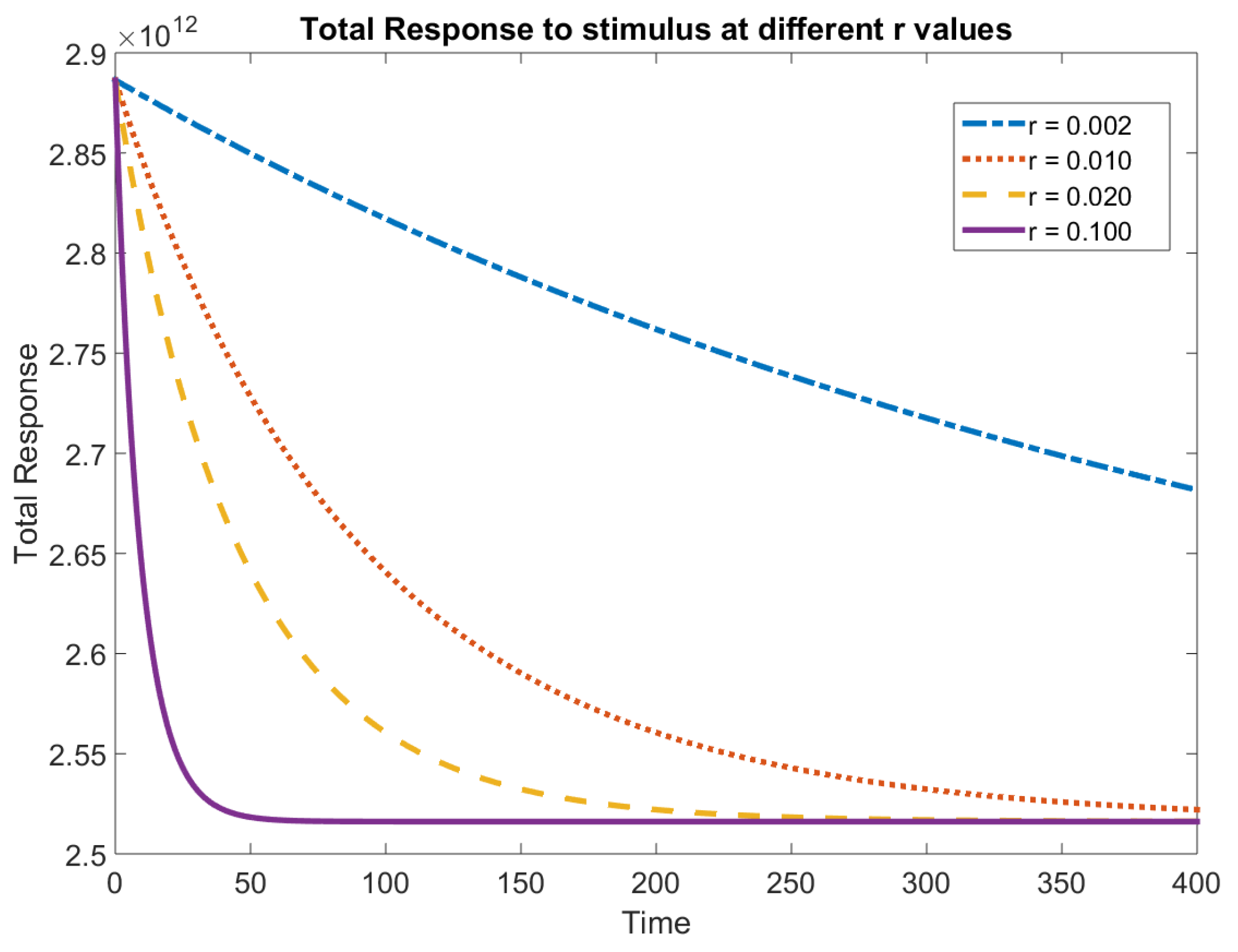
We observe the same dynamics when we alternate the intrinsic growth rate of consumption, r. The responses to the stimuli converge into the range 2.5–$2.55\times {10}^{12}$ for the parameter values in Table 1.

4. Discussion and Conclusions

By applying OPT to consumer behavior during a financial crisis, this study models the short-term surge in consumer spending followed by subsequent economic adjustments. Using differential equations to represent these processes, the paper offers valuable insights into the intricate interplay between immediate policy interventions and longer-term economic repercussions.

Focusing specifically on the United States’ response to the 2008 Global Financial Crisis, this study reveals evidence of a diminishing response to prolonged stimulus. Factors contributing to this trend include demand saturation, inefficiencies in resource allocation, and agent adaptation. Despite the initial efficacy of monetary stimuli, their prolonged application may lead to adverse effects, such as debt inflation and price escalation, outweighing their benefits as shown in Figure 4, Figure 5 and Figure 6. Furthermore, structural issues persist despite continued stimulus efforts.

Economic stimuli typically aim to enhance consumption, and when modeled mathematically, this results in functions that grow over time. The integral of such a consumption function would logically represent the cumulative effect of these growth dynamics. Result 1 resonates well with the economic theories of Keynesian economics, endogenous growth theory, and the permanent income/life-cycle hypotheses suggest that effective economic stimuli can lead to increasing consumption over time. Keynesian theory’s multiplier effect indicates that initial government spending can trigger further rounds of spending and consumption [26]. Endogenous growth theory posits that investments in human capital and innovation can drive sustained economic growth and higher incomes, boosting consumption [27,28]. The permanent income and life-cycle hypotheses suggest that consumers will increase spending if stimuli raise their expected lifetime income [29,30].

Result 2 indicates a dynamic process in which the effects of economic stimuli on consumption gradually wane, leading to a long-term equilibrium characterized by consumption efficiency driven by underlying economic factors. The diminishing effect of economic stimuli over time aligns with the principles of rational expectations theory, where individuals form expectations about future economic variables based on all available information. As individuals continually update their expectations in response to new information, the impact of stimuli on consumption gradually diminishes [31]. Similarly, consumption convergence towards efficiency is a key aspect of dynamic stochastic general equilibrium (DSGE) models. These models offer a comprehensive framework for analyzing intertemporal dynamics in consumption and other economic variables. By incorporating concepts such as consumption smoothing and long-run equilibrium, DSGE models provide insights into how consumption behavior adapts over time in response to various economic stimuli [32].

This study’s findings align with endogenous growth theory by highlighting the importance of sustainable internal economic activities and efficient resource allocation for long-term growth. The results also reflect the permanent income/life-cycle The hypotheses, showing that while stimuli can boost spending temporarily, long-term consumption adjusts based on expected lifetime income. Additionally, the observed initial increase in spending due to monetary stimuli supports Keynesian principles, illustrating the role of government intervention during downturns, but also indicating that the effectiveness of such measures may diminish over time due to structural issues and changing consumer confidence. Future work includes modeling the consumption dynamics as a random process using stochastic differential equations. Also, one can consider applying delay differential equations to accommodate the reaction time between the activation of the stimulus and the actual consumption.

Future research on applying opponent process theory (OPT) to consumer behavior during the GFC can leverage stochastic modeling and econometric methods for deeper insights. Stochastic modeling, using stochastic differential equations, can capture the randomness and variability in consumer responses, reflecting the initial positive response and subsequent negative adjustments. Econometric methods, such as time series analysis and vector autoregression (VAR), can empirically validate the OPT framework, quantifying the immediate and lagged effects of fiscal stimuli on consumer spending. Integrating these approaches will provide robust insights into consumer behavior dynamics, enhancing OPT’s theoretical framework and informing adaptive economic policy-making. Additionally, wavelet analysis can be used to characterize non-stationary time series, such as those observed in epidemiological data, offering insights into the multi-scale temporal dynamics of consumer behavior during economic crises.