Some Comments about Zero and Non-Zero Eigenvalues from Connected Undirected Planar Graph Adjacency Matrices

Abstract

Two linear algebra problems implore a solution to them, creating the themes pursued in this paper. The first problem interfaces with graph theory via binary 0-1 adjacency matrices and their Laplacian counterparts. More contemporary spatial statistics/econometrics applications motivate the second problem, which embodies approximating the eigenvalues of massively large versions of these two aforementioned matrices. The proposed solutions outlined in this paper essentially are a reformulated multiple linear regression analysis for the first problem and a matrix inertia refinement adapted to existing work for the second problem.

1. Introduction

This paper addresses two related linear algebra-based graph theory problems involving a binary 0-1 symmetric adjacency matrix, say C, representing connected undirected planar graphs with no self-loops, relevant to spatial statistics/econometrics that is generalizable to other especially applied matrix and linear algebra situations. Both pertain to the inertia of a matrix (i.e., its number of negative, zero, and positive—respectively, n₋, n₀, and n₊—eigenvalues, say λ_i(C), i = 1, 2, … , n; e.g., see [1,2]; for a “matrix inertia theory and its applications” exposition, see Chapter 13 in Lancaster and Tismenetsky [3]). Its novelty is twofold within the context of planar graph theory: it contributes knowledge to help fill an existing gap in graph adjacency matrix nullity― the multiplicity of the zero eigenvalue in a graph adjacency matrix spectrum―theory (e.g., [4,5,6,7,8]); and, it adds to the scant literature published to date about matrix inertia (e.g., [9]). The first problem, which goes beyond the well-known solutions for simply calculating zero eigenvalues, concerns enumeration of linearly dependent adjacency matrix column/row subsets affiliated with these zero eigenvalues (e.g., see [10]), a single challenge here as a result of symmetry. The second problem concerns approximation of the real eigenvalues (e.g., see [11]) of these adjacency matrices, particularly their row-standardized version, say W, a linearly transformed version of a Laplacian matrix, that enjoys extremely popular usage in spatial statistics/econometrics applications and conceptualization nomenclature.

With regard to the first dilemma, discussion posted on the internet (see, for example: https://www.mathworks.com/matlabcentral/answers/574543-algorithm-to-extract-linearly-dependent-columns-in-a-matrix (accessed on 24 October 2023); https://stackoverflow.com/questions/28816627/how-to-find-linearly-independent-rows-from-a-matrix (accessed on 24 October 2023); and, https://stackoverflow.com/questions/28928893/linear-dependent-rows-huge-sparse-matrix (accessed on 24 October 2023)) suggests the existence of inadequate understanding about identifying a complete suite of (most likely non-unique) linearly dependent p-tuple, p ≥ 2, subsets of adjacency (or other square) matrix (a finite collection of matrix columns/rows in the same vector space is linearly dependent if some non-zero scalar multiples of them sum to the zero vector; for the simplest 2-tuple case and a graphic theoretic adjacency matrix, identical pairs are easily identified by a brute force non-zero element-by-element comparison algorithm) columns/rows, even if the number of zero eigenvalues is known or calculated. The proposed solution here exploits statistical linear regression estimation theory. Meanwhile, the second difficulty spotlights the desire for a refinement of an approximation offered by Griffith and Luhanga [12] paralleling the regular square lattice (e.g., see [13]) solution by Griffith [14]. Partly stimulating this inclination is an increasing availability of readily accessible high quality fine geographic resolution data for national landscapes partitioned into irregular tessellations, such as census tract or block group polygons for the United States (US), and dissemination area and block polygons for Canada (see https://www.census.gov/geographies/reference-files/time-series/geo/tallies.html (accessed on 24 October 2023) and https://www12.statcan.gc.ca/census-recensement/2021/geo/sip-pis/boundary-limites/index2021-eng.cfm?Year=21 (accessed on 15 June 2022), to name some of the germane countries, whose numbers are in the tens-of-thousands to millions; e.g., 84,414 census tracts and 8,132,968 block groups for the US in 2020, and 57,932 dissemination areas and 498,547 blocks for Canada in 2021. In other words, a substantial applied mathematics demand already exists for solving these two problems.

2. Background to the Pair of Problems

Let G_n = (V, E) be a simple undirected connected graph with n vertices V = {v₁, … , v_n}, and m ≤ n(n − 1)/2 edges E = {e_ij linking vertices v_i and v_j: i = 1, 2, … , n and i = 1, 2, … , n; i ≠ j due to the absence of self-loops}. Often in spatial statistics/econometrics, G_n is both complete and planar, and hence m ≤ 3(n − 2); sometimes G_n is near-planar, with m ≤ 8n. Several well-known properties of the sparse adjacency matrices for these graphs pertaining to both their zero and non-zero eigenvalues include:

(1)

the number of zero eigenvalues count linearly dependent column/row subsets (e.g., [15]);

(2)

the interval [$\underset{1\le \mathrm{i}\le \mathrm{n}}{\mathrm{MAX}}\{\sqrt{\sum _{\mathrm{i}=1}^{\mathrm{n}}{\mathrm{n}}_{\mathrm{i}}^2/\mathrm{n}},\sum _{\mathrm{i}=1}^{\mathrm{n}}{\mathrm{n}}_{\mathrm{i}}/\mathrm{n}\}$, $\underset{1\le \mathrm{i}\le \mathrm{n}}{\mathrm{MAX}}\{\left(1+\sqrt{4{\mathrm{n}}_{\mathrm{j}|\mathrm{i}}-4{\mathrm{n}}_{\mathrm{i}}+1}\right)/2\}$] (e.g., [16,17]) contains the principal eigenvalue (i.e., spectral radius) of the graph G_n adjacency matrix C, where n_i is the ith row sum, and n_j|i is the sum of vertex i’s linked row sums n_j;

(3)

adding a link to graph G_n strictly increases its adjacency matrix C principal eigenvalue(e.g., [18]), whereas removing a link decreases the magnitude of this eigenvalue (e.g., [19]);

(4)

the principal eigenvalue of matrix W is one (via the Perron-Frobenius theorem (e.g., [20]));

(5)

the extreme maximum eigenvalue of matrix C, and the extreme negative eigenvalue of matrix W, for graph G_n compute very quickly [21];

(6)

the variance of the eigenvalues of matrix C is 1^TC1/n, and of matrix W is 1^TD⁻¹C D⁻¹1/n, where 1 is an n-by-1 vector of ones, superscript T denotes the matrix transpose operator, and D is a diagonal matrix whose (i, i) cell entry is n_i [21];

(7)

the sum of the positive eigenvalues equals minus the sum of the negative eigenvalues [all diagonal entries of matrix C are zero in the absence of self-loops, implying that $\sum _{\mathrm{i}=1}^{\mathrm{n}}{\mathsf{\lambda }}_{\mathrm{i}}$ (C) = 0];

(8)

the sum of the k largest eigenvalues of matrix C is at most (√k + 1)n/2 [22];

(9)

the line graph, L(G_n), furnishes a lower bound, whereas the maximally connected graph [23], L(G₂) + L(G_n−2), furnishes an upper bound configuration for numerical planar graph eigenfunction analysis;

(10)

for irregular graphs G_n (i.e., n_i has a relatively small modal frequency coupled with a relatively large range), the theoretical maximum number of negative eigenvalues is 3n/4 [24], whereas empirically this maximum number almost always is less than 2n/3, and usually between n/2 and 3n/5 [25], even in the presence of numerous completely connected K₄ (in graph theory parlance) subgraphs (i.e., the maximum fully connected subgraph Kuratowski’s theorem allows to exist in a planar graph);

(11)

a bipartite graph is always 2-colorable (i.e., one only needs to assign at most two different colors to all graph vertices such that no two adjacent vertices have the same color), and vice-versa (see [26]), implying knowledge about the number and positioning of K₄ subgraphs potentially is informative; and,

(12)

if the maximum degree (i.e., n_i; see property #2) Δ > 3, η denotes nullity, and G_n is not complete bipartite, then η < (Δ − 2)n/(Δ − 1) [5]―this is not a very useful spatial statistics/econometrics upper bound since most irregular surface partitionings have at least one polygon areal unit with Δ sufficiently large (e.g., in the range 10–28) that (Δ − 2)/(Δ − 1) is close to one.

Although this list is not exhaustive, and hence could contain many more eigenvalue properties, these twelve provide a foundation for the findings summarized in this paper. They also highlight that missing from this list is an effective method for determining the set of zero eigenvalues for an adjacency matrix, one of this matrix’s three inertia counts.

Mohar’s [22] result (i.e., property #8) needs modification in order to translate it from matrix C to matrix W. Although the line graph, L(G_n) (i.e., property #9) gives a lower bound configuration for practical spatial statistical problems, an undirected star graph (i.e., K₁ in graph theory parlance) gives its absolute lower bound for the sum of positive eigenvalues, which is one for matrix W; this particular graph also highlights the importance of accounting for zero adjacency matrix eigenvalues. In other words, given that the largest eigenvalue, λ₁(W), equals 1, the upper bound for the k positive eigenvalues is k, denoted here by matrix inertia notation n₊; realization of this value is infeasible for a connected L(G_n) since all non-principal positive eigenvalues other than λ₁(W) are guaranteed to be < 1. Thus, for other symmetric eigenvalue distributions (e.g., those characterizing a regular square tessellation lattice forming a complete rectangular region), this loose upper bound also is n/2 at most, and actually is closer to n₊/2; such a tessellation forming a complete √n-by-√n square region, for a perfect square number n, with links in its dual planar graph defined by pixels sharing a non-zero length boundary, also has √n zero eigenvalues (e.g., see Comellas et al., 2008), slightly reducing this upper bound for it by a factor of (1 − 1/√n). Meanwhile, the sum of positive L(G_n) eigenvalues is approximately/exactly (depending upon whether n is even or odd) equal to $\left\{1+\mathrm{S}\mathrm{I}\mathrm{N}\left[\frac{2\mathrm{k}-1}{2(\mathrm{n}-1)}\mathsf{\pi }\right]/\mathrm{S}\mathrm{I}\mathrm{N}\left[\frac{\mathsf{\pi }}{2(\mathrm{n}-1)}\right]\right\}/2$, implying a sharper upper bound on k for the sum of its first k positive eigenvalues, and n/3—which can be <k—for the sum of all of its positive eigenvalues. This outcome suggests the following more general proposition:

Conjecture 1. 

Let G_n = (V, E) be a simple connected undirected planar graph with n vertices V = {v₁, … , v_n}, and m ≤ n(n − 1)/2 edges E = {e_ij linking vertices v_i and v_j: i = 1, 2, … , n and j = 1, 2, … , n; i ≠ j}. For n ≥ 100 nodes and no self-loops, k  is an upper bound for the sum of the first k positive eigenvalues of its row-standardized adjacency matrix W.

Rationale. 

By the Perron-Frobenius theorem, λ₁(W) = 1, and all other positive eigenvalues in this case are such that 0 < λ_j(W) < 1, j = 2, 3, … , k. Taliceo and Griffith [25] synthesize simulation experiment calculations that suggest a minimum value of around 100 for n, the part of this conjecture requiring proof. Tait and Tobin [23] underline the potential for G_n displaying anomalous qualities when n is small, noting that the maximum connectivity case requires n to exceed 8 to be true. Furthermore, in their extensive investigation of planar graphs housing embedded K₄ subgraphs, Taliceo and Griffith [25] reveal that 3n/4 negative eigenvalues occur, at least asymptotically with increasing n, for certain supra-structure wheel and line graphs organizing a substructure of only K₄ subgraphs, which is a peculiarity vis-à-vis empirical surface partitionings. Their empirical inventory, together with the observational roster appearing in

Table 1. Selected chosen specimen geographic landscape surface partitioning descriptors (also see Appendix A).

Geographic Landscape	n	K4 Count	Matrix C					Matrix W
			UB	λ1(C)	LB	λn(C)	1TC1	λ2(W)	λn(W)
England †	839	9	7.59	6.07	4.97	−4.19	3564	0.9976	−0.93
Chicago ‡	2067	35	8.52	6.22	5.30	−3.73	10,562	0.9987	−0.86
Edmonton §	2098	121	10.95	6.95	5.62	−4.32	10,640	0.9985	−0.77
North Carolina ‡	2195	52	8.52	6.28	5.77	−3.76	12,206	0.9994	−0.70
US HSA ⁑	3408	204	12.13	7.82	5.94	−4.46	18,308	0.9996	−0.96
Texas ‡	5265	185	12.43	7.43	5.66	−4.52	28,176	0.9995	−0.84
Syracuse †	7249	322	12.30	7.38	5.40	−5.02	35,100	0.9994	−0.94

NOTE: n denotes the number of graph G_n nodes; K₄ denotes the well-known completely connected G₄; λ denotes eigenvalue; UB/LB denote upper/lower bound; ^§ Statistics Canada 2011 census tracts; ^⁑ US HSA denotes 2017 US hospital service areas.; ^† Appears in Griffith and Luhanga (2011). ^‡ US Census Bureau 2000, 2010, or 2020 census tracts.

(also see Appendix A), implies that most irregular surface partitions have a relatively small percentage of their edges arranged in the precise formation of these subgraphs.

The rare event nature of this preceding K₄ situation reflects upon a need to adequately differentiate theoretical and practical consequences.

The principal eigenvalue λ₁(C) upper bound result proved and reported by Wu and Liu [17] can extend this conjecture to binary 0-1 graph adjacency matrices with an improved bound of k$\times \underset{1\le \mathrm{i}\le \mathrm{n}}{\mathrm{MAX}}\{\left(1+\sqrt{4{\mathrm{n}}_{\mathrm{j}|\mathrm{i}}-4{\mathrm{n}}_{\mathrm{i}}+1}\right)/2\}$ < (√k + 1)n/2. This value outperforms even the extreme negative eigenvalue case of k = n/4 for all positive eigenvalues: for example, using the true n₊ value, (7.59)(839)/2 (≈3184.05) is closer than (√393 + 1)(839)/2 (≈ 8738.76) to 656.86, the ensuing empirical England illustration numbers.

Finally, while a λ_n(W) value of −1 implies the foregoing loose upper bound of n/2, as λ_n(W) goes toward its smallest absolute value of roughly −1/2 (e.g., [27]), property #10 implies that this loose upper bound goes to n/4. One implication here is that λ_n(W) can either directly or indirectly contribute to establishing sharper upper bounds. Taliceo and Griffith [25] reveal that values greater than the extreme case of −1 move the loose upper bound toward 2n/5. This hypothesis merits future research attention. Therefore, as the discussion in this section reflects, a prominent theme in the existing literature concerns various aspects of positive eigenvalues, relegating negative eigenvalues to a secondary topic, while nearly ignoring zero eigenvalues altogether.

3. Specimen Empirical Surface Partitionings and Their Dual Graphs

Although the first problem this paper addresses entailing subsets of linearly dependent columns/rows appears to be of interest for any size matrix (e.g., Appendix B furnishes an easily replicated and control example, suitable for launching exploratory work, with much known about its zero eigenvalues for any size adjacency matrix), the second entailing eigenvalue approximations is of pragmatic interest—beyond verification exercises—especially in spatial statistics/econometrics, and only for extremely large matrices involving n in the 100,000s or greater (i.e., matrices for which numerical computation of eigenvalues is prohibitive in terms of time or computer memory requirements that surpass ultramodern resource capabilities). This section treats a relatively large n that is much smaller than this restrictive magnitude, but sufficiently large to engage computational challenges while allowing comparisons with accurate numerical solutions, namely n between 839 and 7249. The seven selected cases are actual real-world surface partitionings, with their selection decisions partly attributable to their relative and absolute sizes. Table 1 summarizes some of their relevant features. Its upper bound for λ₁(C) exhibits a marked decrease—by an average of over 50%—from the maximum n_i values delivered by the Perron-Frobenius theorem.

Figure 1 portrays the selected empirical eigenvalue distributions. The complete sets of eigenvalues tend to resemble, and somewhat align with, truncated gamma probability density function distributions. The positive eigenvalue subsets more closely resemble skewed Weibull distributions (with most of the analyzed cases here displaying conspicuous tail deviations). These subset graphics help visualize the aforementioned conjecture.

Table 2. Selected descriptors of the chosen specimen geographic landscape surface partitionings containing zero λs.

Feature	Removed λ = 0	England	Edmonton	US HSA	Texas	Syracuse
λ1(C)	none	6.071787	6.950707	7.820136	7.431868	7.375069
	2-tuples	6.027092	6.905243	7.820136	7.413686	7.352621
	p-tuples	6.026312	6.886547	7.820136	7.406109	7.352365
λn(C)	none	−4.185268	−4.324066	−4.458946	−4.523357	−5.024567
	2-tuples	−3.729453	−4.236484	−4.353676	−4.512665	−5.018984
	p-tuples	−3.729440	−4.236477	−4.353676	−4.506244	−5.017506
λn(W)	none	−0.925413	−0.773818	−0.956681	−0.843875	−0.935861
	2-tuples	−0.900969	−0.731063	−0.956681	−0.843875	−0.935861
	p-tuples	−0.900969	−0.728697	−0.956681	−0.843875	−0.935861
1TC1	none	3564	10,640	18,308	28,176	35,100
	2-tuples	3400	10,584	18,294	28,142	34,932
	p-tuples	3372	10,536	18,290	28,126	34,878
1TD−1C D−11	none	177.14	397.38	620.01	977.65	1440.31
	2-tuples	165.02	394.03	619.06	976.71	1434.92
	p-tuples	161.61	391.09	618.58	976.35	1431.56
p-tuple frequency	2	79	23	6	7	48
	3	5	0	1	1	7 †
	4	3	4	1	2	9
	5	4	4	0	0	3
	6	1	1	0	0	1
	7	0	1	0	0	0
	8	0	0	0	0	2
	10	2	0	0	0	0
	11	1	0	0	0	0

NOTE: λ denotes eigenvalue; ^† one 2-tuple overlaps with, and hence may mask, two 3-tuples.

presents a second tabulation with entries for the five selected empirical adjacency matrices containing zero eigenvalues. These recordings insinuate that 2-tuples may be the dominant source of zero eigenvalues in empirical graph adjacency matrices (also see Appendix Figure A1), an anticipation consistent with intuition. The affiliated zero eigenvalues are a straightforward consequence:

Lemma 1. 

If each of two nodes in a graph has a single link that connects them only with a common other node, then this graph’s binary 0-1 adjacency matrix C has a zero eigenvalue.

Proof. 

Without loss of generality, arrange an adjacency matrix such that the two nodes in question occupy the first and second column/row positions of the adjacency matrix under study. Utilizing elementary matrix determinant column/row operations (e.g., [28,29]), subtracting the second row from the first row of det|(C − λI)|, where det denotes matrix determinant, and then adding the first column to the new second column, yields.

$$\mathrm{d}\mathrm{e}\mathrm{t}\left|\left(\begin{array}{ccc}-\mathsf{\lambda }& 0& \begin{array}{ccc}\mathbf{0}& 1& \mathbf{0}\end{array}\\ 0& -\mathsf{\lambda }& \begin{array}{ccc}\mathbf{0}& 1& \mathbf{0}\end{array}\\ \begin{array}{c}\mathbf{0}\\ 1\\ \mathbf{0}\end{array}& \begin{array}{c}\mathbf{0}\\ 1\\ \mathbf{0}\end{array}& {\mathbf{C}}_{\mathrm{n}-2,\mathrm{n}-2}\end{array}\right)\right|=\det \left|\left(\begin{array}{ccc}-\mathsf{\lambda }& 0& \begin{array}{ccc}\mathbf{0}& 0& \mathbf{0}\end{array}\\ 0& -\mathsf{\lambda }& \begin{array}{ccc}\mathbf{0}& 1& \mathbf{0}\end{array}\\ \begin{array}{c}\mathbf{0}\\ 1\\ \mathbf{0}\end{array}& \begin{array}{c}\mathbf{0}\\ 2\\ \mathbf{0}\end{array}& {\mathbf{C}}_{\mathrm{n}-2,\mathrm{n}-2}\end{array}\right)\right|$$

(1)

Next, implementing the Laplacian expansion by minors for cell entry (1, 1) renders λ = 0. This result is corroborated by the determinant property that the eigenvalues of a block diagonal matrix are the union of the individual block matrix eigenvalue sets. □

Corollary 1. 

Lemma 1 applies to K > 1 separate distinct pairs of nodes in a graph that have a single link connecting each of a duo only with another common node.

Proof. 

Without loss of generality, arrange an adjacency matrix such that the K pairs of nodes in question contiguously occupy its first 2K column/row positions, reducing the core adjacency matrix to C_{n−2K,n−2K}. Recursively applying the Lemma 1 proof technique to the K twosomes yields K zero eigenvalues. □

Lemma 2. 

If each of K nodes in a graph has a single link that connects them only with a common other node (i.e., a star graph, a special case of a complete bipartite graph), then this graph’s binary 0-1 adjacency matrix C has at least K − 1 zero eigenvalues.

Proof. 

Without loss of generality, arrange an adjacency matrix such that the K nodes in question contiguously occupy its last K column/row positions, reducing the core adjacency matrix to C_n−K,n−K. Then,

$$\begin{gathered} \mathrm{d}\mathrm{e}\mathrm{t}\left|\left(\begin{array}{cc}{\mathbf{C}}_{\mathrm{n}-\mathrm{K},\mathrm{n}-\mathrm{K}}-\mathsf{\lambda }{\mathbf{I}}_{\mathrm{n}-\mathrm{K}}& \begin{array}{c}{\mathbf{0}}_{\mathrm{n}-\mathrm{K}-1,\mathrm{K}}\\ {\mathbf{1}}_{\mathrm{K},1}^{\mathrm{T}}\end{array}\\ \begin{array}{cc}{\mathbf{0}}_{\mathrm{K},\mathrm{n}-\mathrm{K}-1}& {\mathbf{1}}_{\mathrm{K},1}\end{array}& -\mathsf{\lambda }{\mathbf{I}}_{\mathrm{K}}\end{array}\right)\right|= \\ \mathrm{d}\mathrm{e}\mathrm{t}\left|\left(\begin{array}{cc}{\mathbf{C}}_{\mathrm{n}-\mathrm{K},\mathrm{n}-\mathrm{K}}-\mathsf{\lambda }{\mathbf{I}}_{\mathrm{n}-\mathrm{K}}& \begin{array}{c}{\mathbf{0}}_{\mathrm{n}-\mathrm{K}-1,\mathrm{K}}\\ \begin{array}{cc}1& {\mathbf{0}}_{\mathrm{K}-\mathrm{1,1}}^{\mathrm{T}}\end{array}\end{array}\\ \begin{array}{cc}{\mathbf{0}}_{\mathrm{K},\mathrm{n}-\mathrm{K}-1}& \begin{array}{c}1\\ {\mathbf{0}}_{\mathrm{K}-\mathrm{1,1}}\end{array}\end{array}& \begin{array}{cc}\left(\mathrm{K}-1\right)-\mathsf{\lambda }& {\mathbf{0}}_{\mathrm{K}-\mathrm{1,1}}^{\mathrm{T}}\\ {\mathbf{0}}_{\mathrm{K}-\mathrm{1,1}}& -\mathsf{\lambda }{\mathbf{I}}_{\mathrm{K}-1}\end{array}\end{array}\right)\right| \end{gathered}$$

(2)

Next, implementing the Laplacian expansion by minors for the ending (K − 1)-by-(K − 1) cell entries, −λ_K−1, is equivalent to applying it to a star graph for which one of its nodes is contained in the core adjacency matrix, C_n−K,n−K, rendering at least K − 1 zero eigenvalues (see [30], p. 266). □

Corollary 2. 

If each of K nodes in a square mesh lattice (i.e., regular square tessellation) graph has a single link that connects them only with a common other node (i.e., a star graph), then this graph’s binary 0-1 adjacency matrix C has at least P + K − 2 zero eigenvalues.

Proof. 

Extending the proof for Lemma 2, the core adjacency matrix, C_n−K,n−K = ${\mathrm{C}}_{{\mathrm{P}}^2,{\mathrm{P}}^2}$ for a P-by-P regular square tessellation, in isolation has P zero eigenvalues for its rook adjacency definition―its eigenvalues are given by 2{COS[πj/(P + 1)] + COS[πk/(P + 1)]}, j = 1, 2, … , P and k = 1, 2, … , P [31], with the P cases of k = [(P + 1) – j] yielding zero values. One of these matches occurs for each integer j, yielding a total of P zero eigenvalues. But the single arbitrary node to which the star graph attaches has its column/row modified by its P + 1 column and row additional entries that render the matrix determinant

$$\det \left|\left(\begin{array}{cc}{\mathbf{C}}_{{\mathrm{P}}^2,{\mathrm{P}}^2}-\mathsf{\lambda }{\mathbf{I}}_{{\mathrm{P}}^2}& \begin{array}{c}{\mathbf{0}}_{{\mathrm{P}}^2-1,1}\\ 1\end{array}\\ \begin{array}{cc}{\mathbf{0}}_{1,{\mathrm{P}}^2-1}& 1\end{array}& \left(\mathrm{K}-1\right)-\mathsf{\lambda }\end{array}\right)\right|,$$

(3)

and hence removes one of the P zero eigenvalues. Hence, the number is P − 1 + K − 1 = P + K − 2. □

Remark. 

This corollary produces an exact expectation for algorithm and conjecture verification exercises like the simulation specimens outlined in Appendix B.

Corollary 3. 

If each of H sets of K_h nodes forms a separate, distinct star subgraph, then this graph’s binary 0-1 adjacency matrix C has at least $\sum _{\mathrm{h}=1}^{\mathrm{H}}{\mathrm{K}}_{\mathrm{h}}$ – H zero eigenvalues.

Proof. 

Recursively applying the Lemma 2 proof technique to the H collections of K_h nodes yields $\sum _{\mathrm{h}=1}^{\mathrm{H}}{\mathrm{K}}_{\mathrm{h}}$ – H zero eigenvalues. □

Remark. 

These star subgraphs need to attach to nodes that contribute to linear combinations of the core adjacency matrix ${\mathrm{C}}_{\mathrm{n}-\sum _{\mathrm{h}=1}^{\mathrm{H}}{\mathrm{n}-\mathrm{K}}_{\mathrm{h}},\sum _{\mathrm{h}=1}^{\mathrm{H}}{\mathrm{K}}_{\mathrm{h}}}$ in order to eliminate one of its zero eigenvalues (see Corollary 2 proof).

• Table 2 entries also raise questions about the claim by Feng et al. [18] that adding links strictly increases the matrix C principal eigenvalue’s magnitude (e.g., the US HAS specimen graph), which is the reason this table’s entries show so many decimal places; rather, this spectral radius amount looks to be simply monotonically non-decreasing. This assertion may well apply to the extreme negative eigenvalues, too: they also appear to be monotonically increasing in absolute value.

The p-tuples acknowledged in Table 2 are the linearly dependent subsets of columns/rows producing zero eigenvalues in their respective adjacency matrices. The next section discusses a statistical regression estimation operator mechanism for uncovering these linear combinations. Their important attributes alluded to in this table include overlaps (i.e., a column/row can be a member of more than one linearly dependent subset), size variation (i.e., the number of columns/rows in a linear combination equation), and frequency that seems to decrease with increasing size, perhaps mirroring a Poisson distribution. Overlaps emphasize that the discovered p-tuples acknowledged in Table 2 are not necessarily unique; those removed for the construction of this table are ones that maintain a connected graph [documented by λ₂(W) ≠ 1] as well as contain the smallest possible n_is (most often just one).

4. Identifying Linearly Dependent Column/Row Subsets in Adjacency Matrices

Hawkins [32] gives an insightful clue to identifying linearly dependent column/row subsets in an adjacency matrix by noting that eigenvectors of (near-)zero principal components extracted from a correlation matrix constructed by amalgamating a dependent variable and its accompanying set of covariates suggest possible alternative sub-regressions. One weakness of his conceptualization occurs with multiple zero eigenvalues: their eigenspace is not unique [33,34], and hence is an arbitrary choice among all of the possible correct eigenvectors for a repeated (non-degenerate) eigenvalue from a real symmetric matrix. Consequently, if only a few zero eigenvalues exist, then multivariate principal components analysis (PCA) tends to recover p-tuples like the simple structure ones referenced in Table 2 acquired with the SAS PROC TRANSREG [35] procedure. Otherwise, it can confuse even the stand-alone 2-tuple sources. Accordingly, still pursuing this regression approach, standard linear regression procedures designed to detect and convey a user message equivalent to “model is not of full rank” (e.g., the SAS PROC REG [35] message) furnishes a process that yields the desired p-tuples.

Overlapping linear combinations constitute a complication whose astute management and treatment remain both elusive and a fruitful subject of future research. The Syracuse entry in Table 2 as well as Appendix C underscore some of the data analytic complexities that can arise in the presence of this phenomenon.

4.1. Competing Algorithms

SAS champions the sweep algorithm (aka SWP [35,36], [37] (pp. 95–99), [38]; Tsatsomeros [39] furnishes an excellent literature review and historical overview for it), whereas much contemporary mathematical work advocates for the classical QR with a column pivoting solution (e.g., [40,41,42]). As an aside, Lange ([37], pp. 93–94) notes that “[t]he sweep operator … is the workhorse of computational statistics,” and that “[a]lthough there are faster and numerically more stable algorithms for … solving a least-squares problem, no algorithm matches the conceptual simplicity and utility of sweeping” due to its superior abilities to efficiently and effectively exploit linear regression matrix symmetries; he then notes that its historical competitors were/are the Cholesky decomposition, the Gram-Schmidt orthogonalization, and Woodbury’s formula. Meanwhile, generally speaking, this former QR algorithm, the most serious contemporary competitor of the sweep operator, performs elementary row operations on a system of linear equations, which for least squares regression is the set of normal equations. It enables the execution of this linear regression by sweeping particular rows of the sums-of-squares-and-cross-products matrix X^TX in or out, where sweeping is similar to executing a Gauss-Jordan elimination. This sweep procedure involves the following sequence of matrix row adjustments (the basic row operations, pivoting exclusively on diagonal matrix elements, are the multiplication of a row by a constant, and the addition of a multiple of one row to another) based upon diagonal element h in matrix X^TX = <a_jk> whose nonzero value is c_hh:

• j = k = h: matrix entry X^TX[h, h] = a_hh,
• j = h & k ≠ h: matrix entry X^TX[h, k] = a_hk/a_hh, and
• j ≠ h & k ≠ h: matrix entry X^TX[j, k] = a_jk – a_jha_kh/a_hh.

The row operations generating these quantities simultaneously update estimates for the regression coefficients, error sum of squares, and generalized inverse of the given system of equations. Matrix X^TX symmetry requires calculations for only its upper triangle, reaping execution time savings. It also achieves in-place mapping with minimal storage. Meanwhile, sweeping in and out refers to the reversibility of this operation. These preceding added effects constitute “sweeping in.” They can be undone by sweep a second time, constituting “sweeping out.” This sweep operator is quite simple, making it an extremely useful tool for computational statisticians.

In contrast, a QR algorithm, which tends to be slow but accurate for ill-conditioned systems, applies the QR matrix decomposition (aka QR or QU matrix factorization) of X^TX = QR, where Q is an orthonormal matrix, and R is an upper triangular matrix. The appeal of such an orthogonal matrix is that its transpose and inverse are equal. Thus, the linear regression system of equations X^TXb = (X^TY) reduces to a triangular system Rb = Q^T(X^TY), which is much easier to solve. Implementation of this QR algorithm can be carried out with column pivoting, which bolsters its ability to solve rank-deficient systems of equations while tending to provide better numerical accuracy. However, by doing so, it solves the different system of equations X^TXP = QR, or X^TX = QRP^T, where P is a permutation matrix linked to the largest remaining column (i.e., column pivoting) at the beginning of each new step. The selection of matrix P usually is such that the diagonal elements of matrix R are non-increasing. This system of equations switch potentially adds further complexity to handling this algorithm. Nevertheless, column pivoting is useful when eigenvalues of a matrix actually, or are expected to approach, zero, the topic of this paper. Consequently, the relative simplicity of the sweep algorithm frequently makes it preferable to a QR algorithm.

A systematic comparative review or numerical examination between the sweep operator and its handful of prominent competitors mentioned here is beyond the scope of this paper. The conceptual discussion in this section identifies certain strengths and weaknesses of this sweep operator, which is a reasonable starting point for embarking upon such a future assessment.

4.2. SAS Procedures: REG and TRANSREG

PROC REG [35] sequentially applies a sweep algorithm to the mathematical statistics normal equations formed from the standard linear regression cross-products covariate matrix X^TX, according to the order of the covariates appearing in its SAS input statement. It always begins by sweeping the first column in matrix X, followed by the next column in this matrix if the pivot is less than a near-zero value whose default SAS threshold magnitude is 1.0 $\times$ 10⁻⁹ for most machines (i.e., if that column is not a linear function of the preceding column), then continuing sequentially to each of the next columns if their respective pivots are not less than this threshold amount, until it passes through all of the columns of matrix X. This method is accurate for most undirected connected planar graph adjacency matrixes since they are reasonably scaled and not too collinear. Given this setting, this SAS procedure can uncover linearly dependent subsets of adjacency matrix columns by specifying its first column, C₁, as a dependent variable, and its remaining (n − 1) columns, C₂-C_n, as covariates. SAS output from this artificial specification includes an enumeration of the existing linearly dependent subsets of columns. A second regression that is stepwise in its nature and execution can check whether or not C₁ itself is part of a linear combination subset. Simplicity dissipates here when n becomes too large, with prevailing numerical precision resulting in some linear combinations embracing numerous superfluous columns with computed near-zero regression coefficients (e.g., 1.0 $\times$ 10⁻¹¹). This rounding error corruption emerges in PROC REG [35] between n = 2100 (e.g., the Chicago empirical example) and n = 3408 (e.g., the US HSA empirical example).

In contrast, PROC TRANSREG [35] executes nonsequential sweeps, finding the best column to sweep first, followed by the second best, then the third best, and so on. This deviation from a sequential SAS input ordering tends to be more numerically accurate. Again, simplicity dissipates here when n becomes too large, although a much larger n than that for PROC REG [35], emerging here somewhere between n = 5265 (e.g., the Texas empirical example) and n = 7249 (e.g., the Syracuse empirical example). In such messy situations, which usually are for the larger -tuple values of p, ignoring the near-zero regression coefficients exposes the correct latent subset linear combinations. Therefore, PROC TRANSREG [35] is the SAS procedure most often utilized in this paper, with a few of its smaller n results checked or carried out with PROC REG [35].

4.3. Disclosing Subset Linear Combinations for the Specimen Empirical Surface Partitionings

We denote the columns of a given n-by-n matrix by COLj, j = 1, 2, … , n (i.e., number them from left to right in a matrix with consecutive positive integers). Among other listings, Table 2 details the numbers and sizes of subset linear combinations of the specimen graph adjacency matrix columns, once more understanding that symmetry means row outcomes are exact parallels. Neither the Chicago nor the North Carolina empirical examples contain zero eigenvalues, and their PROC TRANSREG [35] results yield no “less than full rank model” (the PROC TRANSREG message) warning.

Identifying 2-tuples is relatively easy and efficient for an undirected connected planar graph G_n. Since its sparse binary 0-1 adjacency matrix may be stored as a list of no more than 6(n − 2) pairs of edges/links, rather than either a full n² or no-self-loops n(n − 1) set of pairings, a fast comparison of the position of ones in two columns is possible. These revelations, which primarily are the ones Griffith and Luhanga [12] report, can serve as a check for generated regression disclosures. Sylvester’s [43] matrix algebra inertia theorem transfers these linear combinations from matrix C to matrix W.

Figure 2 portrays the SAS output for the Texas empirical example. The order of column appearances in an equation is irrelevant, although switching them between the right- and left-hand sides of the equations can alter the itemized linear combination coefficients, if only in terms of their signs. The seven 2-tuples here corroborate the fast brute force pairwise comparison matchings outcome based upon a sparse adjacency matrix file. In addition, PROC TRANSREG [35] identifies the columns constituting the exclusive 3-tuple (i.e., {C₁₅₉₄, C₁₆₆₈, C₂₄₅₁}) and the two 4-tuple (i.e., {C₃₂₆₃, C₃₂₆₄, C₃₂₆₅, C₃₂₇₀} and {C₄₈₄₂, C₄₈₄₇, C₄₈₄₈, C₄₈₄₉}) subsets.

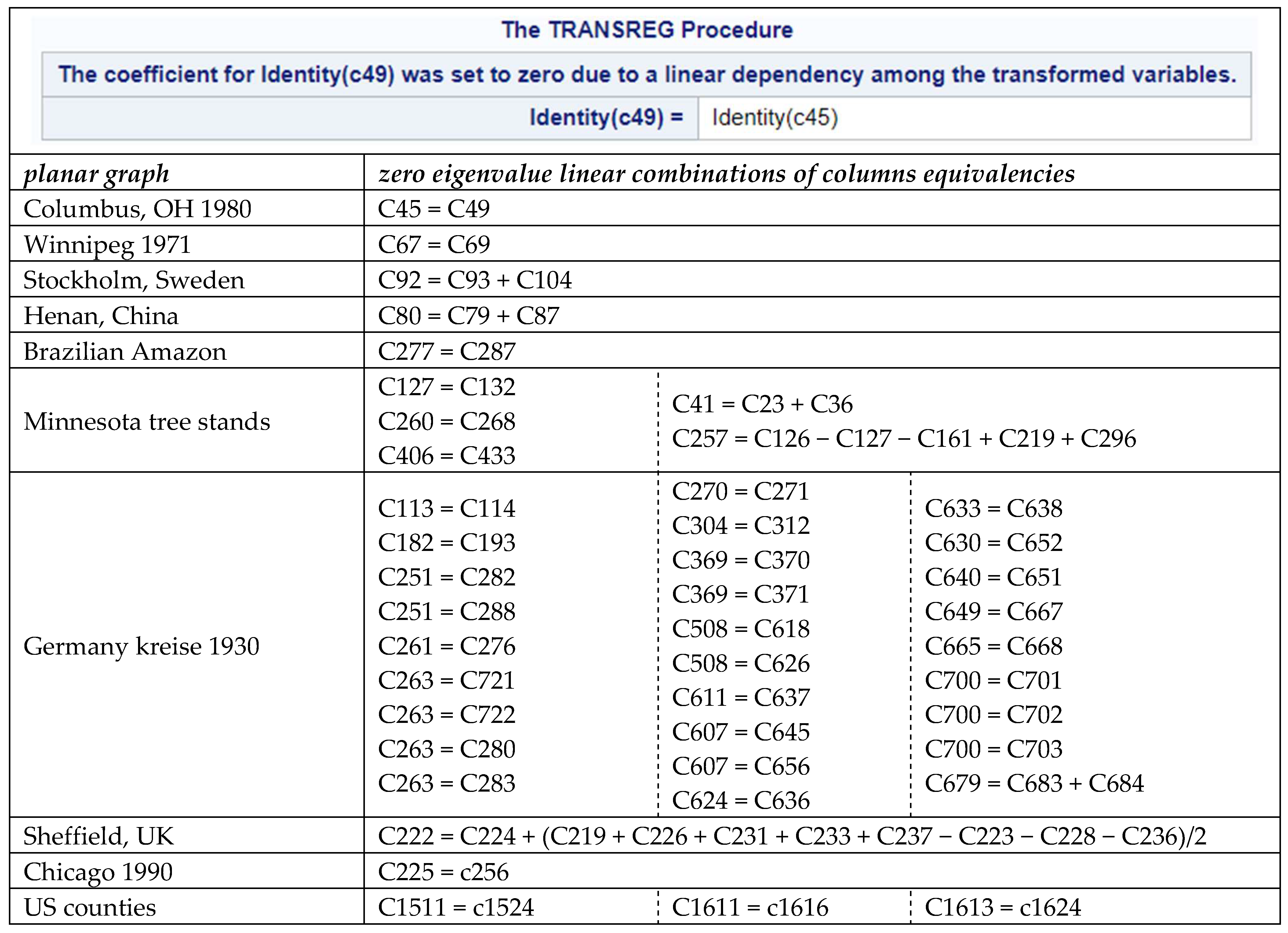
Figure 3 portrays part of the SAS output for the Syracuse empirical example. The near-zero coefficients (e.g., all $\pm$0.000197 or $\pm$0.000031) are unessential (i.e., attributable to numerical imprecision), whereas the few $\pm$1.0000 coefficients indicate the latent subset: C₅₅, C₉₇, and C₁₄₁. The term “Identity” appears in this computer hardcopy since PROC TRANSREG [35] enables and implements variable transformations, with this particular formulation option instructing this procedure to retain the initial untransformed variables themselves.

Figure 4 demonstrates the failure of PCA to always produce simple linear combinations (i.e., simple structure) due to the non-uniqueness of the eigenspaces involved. Multiple linear regression allocates the repeated adjacency matrix column C₁₄₆₀ in this example to only one subset linear combination, whereas PCA introduces some confusion by allocating it to the various subsets to which it also could belong. In other words, the linear regression approach employing a sweep operator furnishes a more parsimonious solution here. One important aspect of this exemplification is that PCA muddling still materializes in the presence of a relatively large n (i.e., 3408) coupled with a quite small number of redundant columns (i.e., eight).

4.4. Discussion: Selected Sweep Operator Properties

Computational complexity and robustness are two salient properties beyond advantages established via competitor algorithm comparisons that demand commentary here supplementing that already appearing in Section 4.1, if for no other reason than to better contextualize the sweep operator within the existing literature. In statistics, although Goodnight [36] popularized this operator, Dempster [44] essentially introduced it to this discipline, with Andrews [45] evaluating it in terms of robustness; noteworthy is that non-statisticians call it by other names, including the principal pivot transform [46], gyration [47], and exchange [48]. Two of its close relatives are the (previously mentioned) Gauss-Jordan elimination ([42], p. 166) and the forward Doolittle ([36], pp. 151–152), an execution step in the LU decomposition, procedures. Thus, on the one hand, its computational complexity—the solution time and memory/storage space resources required by it to solve a specific zero eigenvalue problem—are not extreme, relatively speaking. For example, SAS reports total processing CPU execution time of 5:22.59 for n = 7249 (the largest graph analyzed in this paper) on a desktop computer with four CPUs. It quickly regresses all variables, such as the second through nth columns, against one specified variable, such as the first column, of a graph adjacency matrix, obtaining in a single execution linear regression computations and all perfect linear combinations of columns that are present. Therefore, it is relatively efficient and scalable to the same degree as any linear regression algorithm; linear regression scalability is not computationally heavy.

On the other hand, computer algorithm robustness here—a desirable characteristic ensuring the sweep algorithm maintains reliability and resilience across differing circumstances—refers to its ability to consistently and accurately uncover zero eigenvalue linear combinations of covariates in the presence of various types of disturbances, errors, and/or unexpected inputs (e.g., the random planar graphs of Appendix C). Accordingly, the criteria it must satisfy should ensure that it is able to identify perfect linear combinations that are: (1) for multiple replications of a single adjacency matrix column/row (see Corollary 2); (2) smaller ones embedded in larger ones (e.g., see Table 2); (3) different but sharing columns/rows without double-counting them (e.g., see Figure A1); (4) not confused by numerical precision/rounding error (e.g., see Figure 3); and, (5) for excessively complicated outlier graph structures (e.g., Corollary 2) involving very many columns/rows (see Figure A3). In other words, the sweep operator is resistant since it continues to Identify all latent zero eigenvalue linear combinations even if a small fraction of a graph adjacency matrix undergoes detrimental alterations, or the recovered linear combination is tremendously sophisticated (see Appendix C). With regard to the preceding fourth point, PROC TRANSREG [35] often appears to be more resilient than PROC REG [35], at least in their SAS enactment. However, the reported trivial regression coefficients are so small that they become obvious precision errors (see Section 4.2) to the naked eye.

5. Approximating the Eigenvalues of Matrix W

The spatial statistical problem of interest here is estimation of the auto-normal model normalizing constant (e.g., [49]), the Jacobian of the transformation from a spatially autocorrelated to a spatially unautocorrelated mathematical space using calculus terminology. This quantity almost always is a function of the undirected connected planar graph dual row-standardized adjacency matrix W eigenvalues for a configuration of polygons forming a two-dimensional surface partitioning. Such eigenvalue calculations are possible for quite large n, In the lower 10,000s, but become Impossible beyond the frontiers of computing power, a constantly expanding resource size. This normalizing constant is the existing work adaption target for the matrix inertia refinement this paper disseminates.

An undirected star graph, K_1,n, perceptively illustrates the problem here in its extreme: its eigenvalues are 1, n − 2 0s, and −1 for matrix W, whereas they are $\pm \sqrt{1^{\mathrm{T}}\mathbf{C}1}$ and n − 2 0s for matrix C. In this kind of situation, Bindel and Dong [15], for example, show how eigenvalue frequency distributions can become dominated by a spike at zero (also see Figure 5b,d). A null eigenvalue fails to add any amount to the sum of the n eigenvalues, regardless of the value of n for star graph G_n. For all n > 1, the variance of these eigenvalues is 1^TD⁻¹C D⁻¹1 = 2. More realistic graphs show that although λ₁(W) = 1 remains unchanged, adding redundant links that introduce zero eigenvalues can alter λ_n(C) and λ_n(W) as well as some or all of the intermediate eigenvalues (see Table 2). Furthermore, the matrix W eigenvalues have a more limited range (Table 2) that causes their density to increase faster than it does for their binary 0-1 parent matrix C eigenvalues.

Estimating a complete set of n eigenvalues with a method of moments type technique means spreading the variance over all n values while constraining their sum to equal zero. Griffith and Luhanga [12] address the need to include matrix inertia information in this process: zero eigenvalues should not have non-zero allocations during an approximation routine, and the number of positive and negative eigenvalues needs differentiation in asymmetric eigenvalue distributions since the same cumulative sum almost certainly is spread over fewer individual λs in one of the two instances (almost always the positive domain). Taliceo and Griffith [25] explore this latter trait. Incorporating these two facets for remotely sensed data (e.g., see [13]) analyses renders remarkably accurate eigenvalue approximations for that spatial statistical landscape [14], in part due to its symmetric eigenvalue distribution for the often employed rook adjacency definition. In contrast, ignoring these two influential facets tends to cause typical administrative districts (e.g., counties, census tracts) forming irregular surface partitioning to approximate eigenvalues displaying a discontinuity separation gap at zero (e.g., Figure 5a,c; a finding reported by Griffith in earlier publications). Improved adoption of these two eigenvalue properties should enable a better approximation fabrication for them that exhibits a smoother transition between positive and negative λs.

5.1. Preliminary Eigenvalue Approximation Steps

Eigenvalue approximation can follow a three-step sequence of directives. The first step approximates the extreme eigenvalues of matrices C and W [16,50]. A formulated algorithm employing solely the sparse version of an adjacency matrix (i.e., a sequential listing of only the row-column cells containing a one) quickly produces these values, with extreme accuracy for both λ₁(C) and λ_n(W) (

Table 3. Matrix C and W extreme eigenvalue approximations for the chosen specimen geographic landscape surface partitionings.

Extreme λs	England	Chicago	Edmonton	North Carolina	US HSA	Texas	Syracuse
λ1(C)	6.07179	6.21901	6.95071	6.27921	7.82014	7.43187	7.37507
λn(C)	−4.17990 (−4.18527)	−3.73161 (−3.34868)	−3.88935 (−4.32407)	−3.75641 (−3.75393)	−4.45320 (−4.45895)	−4.52253 (−4.52336)	−3.76275 (−5.02457)
λn(W)	−0.92541	−0.85971	−0.77382	−0.70273	−0.95668	−0.84387	−0.93586

NOTE: λ denotes eigenvalue; actual λ_n(C) values in parentheses, with deviating decimal places in bold font; all λ₁(C) and λ_n(W) reported decimal place values agree.

); the most relevant of these two values for spatial statistics/econometrics is λ_n(W). This algorithm builds its λ_n(C) approximation with the normalized principal eigenvector, E₁, estimated during the iterative calculation of λ₁(C). Next, this algorithm builds its λ_n(W) estimate with the normalized eigenvector E_n approximated during the iterative calculation of λ_n(C). Given that λ₁(W) ≡ 1 is known theoretically, the appealing outcome is that λ_n(W) is knowable for massively large matrices.

The second step of the proposed eigenvalue approximation procedure determines the number of zero eigenvalues. The sparse version of an adjacency matrix also allows a quick identification of all 2-tupes generating zero eigenvalues (

Table 4. Relevant eigenvalue approximation measures for the selected specimen graphs.

Quantity	Category	England	Chicago	Edmon-Ton	North Carolina	US HSA	Texas	Syracuse
tuple small p	2	79	0	23	0	6	7	48
	3	6 †	0	9 †	0	1	2 †	7
inertia	n+	349	891	895	909	1442	2205	3242
	n0	93	0	41	0	8	10	70
	n−	397	1176	1162	1286	1958	3050	3937
exponent	γ	1.4178	1.5656	1.2890	1.2279	2.2820	1.6077	1.8094
	θ	1.3732	1.4636	1.4546	1.4297	1.6744	1.4771	1.6084
λ > 0 bivariate regression	intercept	0.0504	0.0361	0.0348	0.0283	0.0643	0.0419	0.0518
	slope	0.9429	0.9700	0.9643	0.9745	0.9632	0.9684	0.9520
	R2	0.9973	0.9993	0.9992	0.9995	0.9966	0.9988	0.9979

NOTE: λ denotes eigenvalues; 3- and 4-tuples computer execution speed is too slow for massively large graphs; the bivariate regression intercept and slope are close to their respective ideal values of 0 and 1. ^† includes identified overlap matchings with a 2-tuple.

), which in general, and as a rational expectation, seem to account for a preponderance of zero eigenvalues (e.g., [12], Table 1 and Table 2). However, even the triplet computations—executing n(n − 1)(n − 2) trivariate regressions—for the larger of the seven specimen landscapes studied in this paper are too computer intensive for practical purposes. Moreover, presently the best estimate of n₀ is the number of 2-tuples for massively large square matrices. In addition, this approach fails to be effective when extended to more general real matrices since their non-sparseness requires a replacement of each n(n − 1) simple comparison with a bivariate regression; columns/rows can be proportional rather than just equal. This daunting computational demand argues for keeping the original PROC TRANSREG [35] operationalization with its n(n − 1) sweep operations.

The third step approximates the non-zero eigenvalues with a method of moments type of calibration methodology, given that their mean (i.e., zero) and variance (i.e., 1^TD⁻¹C D⁻¹1/n) are either known or easily computable, and hence available. A favored specification for this task exploits eigenvalue ordering by calibrating expressions such as

$$\left.\begin{array}{c}\mathsf{\lambda }\left(\mathbf{W}\right)>0:{\left[\right({\mathrm{n}}_{+}+1–{\mathrm{r}}_{\mathrm{i}})/{\mathrm{n}}_{+}]}^{\mathsf{\gamma }}\\ \mathsf{\lambda }\left(\mathbf{W}\right)<0:{-[\left({|\mathsf{\lambda }}_{\mathrm{n}}\right| {\mathrm{r}}_{\mathrm{i}})/{\mathrm{n}}_{-}]}^{\mathsf{\theta }} \end{array} \right\},$$

(4)

where r_i denotes the descending ordering rank of the i^th eigenvalue after setting aside the set of zero eigenvalues [which subsequently are merged with the approximations generated by Equation (4)], and exponents γ and θ that match the approximated eigenvalue mean and square root of its sum of squares as closely as possible (guided by the method of moments estimation strategy, and using a mean squared error criterion); all manufactured values of expression (4) belong to the interval [0, 1], as do the absolute values of their corresponding actual eigenvalues, with γ > 1 and θ > 1 indicative of variance inflation needing removal, and γ < 1 and θ < 1 indicative of deflated variance needing to be restored. The differences between γ and θ appearing in Table 4 confirm an asymmetric distribution of eigenvalues, whereas the positive eigenvalues bivariate regressions corroborate a well-aligned linear trend with their adjusted rankings. This linear trend tendency is capable of facilitating the drafting of an improved upper bound for the sum of k positive eigenvalues.

5.2. An Instructive Eigenvalue Approximation Assessment

This section summarizes evaluations of two specimen landscapes, namely North Carolina (no zero and 41.4% positive eigenvalues) and Syracuse (48 of 70 easily detectable zero and 45.2% positive eigenvalues). The working assumptions are: (1) the number of 2-tuple zero eigenvalues accurately counts n₀ (the calculable count for massively large G_n), the nearest integer 45% of the non-zero eigenvalues accurately counts n₊ (roughly the mid-point of large-landscape simulation findings reported in [25]), and equation (4) approximates a total set of n eigenvalues. Figure 6 portrays the Jacobian plots across the auto-normal model spatial autocorrelation parameter value contained in its feasible parameter space interval, namely, 1/λ_n(W) < ρ < 1. These graphical findings imply that the enhanced (i.e., refined) but relatively simple eigenvalue approximations proposed in this paper are sufficiently accurate to support sound spatial autoregressive analyses. More comprehensive appraisals of this proposition merit future research attention.

6. Discussion

The following two topics warrant further discussion: identifying linearly dependent subsets of columns/rows in more general matrices, and application of the eigenvalue approximation technique to a very sizeable adjacency matrix.

Table 5. The matrix appearing in both https://stackoverflow.com/questions/11966515/find-all-lineary-dependent-subsets-of-vectors (accessed on 24 October 2023) and https://math.stackexchange.com/questions/182753/find-all-linearly-dependent-subsets-of-this-set-of-vectors (accessed on 24 October 2023), with its rows labeled to indicate its transpose.

	c1	c2	c3	c4	c5	c6
r1	1	1	1	0	1	0
r2	0	0	1	0	0	0
r3	1	0	0	0	0	0
r4	0	0	0	1	0	0
r5	1	1	0	0	1	0
r6	0	0	1	1	0	0
r7	1	0	1	1	0	0

NOTE: c_j denotes column j, and r_j denotes row j; transposing the rows and columns produces the binary rows matrix.

presents a posed problem, one that contains column c₆ that is a trivial zero eigenvalue source, and hence ignored in terms of constructing linear combinations with it. The non-square matrix requires analysis of both its original columns and original rows in their matrix transformed styles. PROC TRANSREG [35] identifies the linearly dependent subsets of columns and rows appearing in Figure 7, with a count of five. Column c₁ and transposed column (i.e., row) r₁ serve as the dependent variables in their respective linear regression analyses. Accordingly, since PROC TRANSREG [35] only uncovers linearly dependent subsets in a collection of covariates, both c₁ and r₁ also have to be analyzed in a stepwise PROC REG [35], which exposes the {r₁, r₂, r₅} linearly dependent subset (e.g., the root mean squared error, _RMSE_, is zero, and the linear regression multiple correlation, _RSQ_, is 1).

The 2010 US census tract polygons covering the entire coterminous continental part of that country furnishes a sizeable empirical example of an undirected connected planar G_n, with n = 72,538, 1^TC1 = 402,830, MAX{n_i} = 48, 1^TD⁻¹C D⁻¹1 = 12985.54, λ₁(C) = 8.63582, and λ_n(W) = −0.89732—desktop computer—Intel(R) Xeon(R) CPU, E5640 @ 2.67GHz and 2.66GHz (2 processors), 24.0GB RAM, 64-bit OS, x64-based processor, Windows 10 Enterprise—execution time for calculating these last two quantities was less than 40 s. Crafting this geographic polygons configuration graph constructed for the coterminous US census tracts irregular surface partitioning involved modifying an ESRI ArcMAP .shp file with such manual adjustments as linking islands to the mainland through ferry routes. The simple 2-tuple matching analysis retrieves 32 zero eigenvalue sources. Consequently, the basic input for approximating the matrix W eigenvalues, and hence the needed Jacobian term for spatial statistical/econometric autoregressive analysis, is not only feasible, but also available here. This exemplification once again illustrates how the matrix inertia refinement promulgated in this paper is adaptable to existing work.

7. Conclusions and Implications

In conclusion, this paper set out to establish solutions to two seemingly unsolved or poorly solved linear algebra problems contained in topics of more general interest, one frequently mentioned on the internet, and the other becoming of increasing interest and concern as geospatial analysts push their empirical spatial statistical/economics analyses to larger and larger georeferenced datasets (sometimes in the realm of machine learning and data mining) and contemporary social network analysts continue to adapt spatial analysis techniques to their often massively larger—the KONECT archive project (http://konect.cc/ (accessed on 24 October 2023) makes 1326 social networks available to the public, ranging in node count from 16 to 105.2 million, of which just 543 have fewer than 10,000 nodes, and whose size frequencies closely conform to a log-normal distribution—denser, and almost certainly non-planar graph generated adjacency matrices. The first is the enumeration of all non-trivial linearly dependent column/row subsets in a matrix. One on-line commentator mentions that this problem most likely requires a supercomputer for even modestly large matrices. The regression-based solution promoted in this paper successfully, efficiently, and effectively handles matrices with dimensions in the 1000s, employing a laptop personal computer using the following processor: Intel(R) Core(TM) i5-2520M CPU @ 2.50 GHz; this machine has 8.00 GB of installed RAM, and runs with a 64-bit operating system, clearly not state-of-the-art computer or supercomputer technology.

The second problem of approximating eigenvalues for massively large matrices builds upon an evolving foundation, with demand for its solution being prompted by the existence of a parallel solution for remotely sensed satellite data whose G_n adjacency matrix size often is in the 10,000,000s [14]. This magnitude echoes that for the aforementioned KONECT project social network entries in excess of one million nodes (reflecting a practical upper limit size), which number 18 and have a median of 30 million nodes, and whose Jacobian term requires the irregular tessellation category of eigenvalue approximations outlined in this paper. Another imperative application arena is the present-day expansion of data mining and machine learning analyses to georeferenced, social media, and other substantially large datasets. The solution advocated for in this paper streamlines earlier results by exploiting extremely large adjacency matrix inertia.

The fundamental implications launched by this paper may be summarized as a combination of the preceding and following conjectures:

Conjecture 2. 

Let G_n = (V, E) be a simple connected undirected planar graph with n vertices V = {v₁, … , v_n}, and m ≤ n(n − 1)/2 edges E = {e_ij linking vertices v_i and v_j: i = 1, 2, … , n and j = 1, 2, … , n; i ≠ j}. If G_n has no K₄ subgraphs, then the maximum value of n₋ is 2n/3.

Conjecture 3. 

Let G_n = (V, E) be a simple connected undirected planar graph with n vertices V = {v₁, … , v_n}, and m ≤ n(n − 1)/2 edges E = {e_ij linking vertices v_i and v_j: i = 1, 2, … , n and j = 1, 2, … , n; i ≠ j}. The sum of the k largest matrix W positive eigenvalues least upper bound for a self-loopless G_n’s adjacency matrix is $\sum _{\mathrm{i}=1}^{\mathrm{k}}\left[\right(\mathrm{n}+1–\mathrm{r}\mathrm{i})/\mathrm{n}+]\mathsf{\gamma }$ + ε for some suitably small ε.

• A more general implication is that geographical analysis matrices continue to be a fertile research subject. Concerted quantitative geography efforts in this area began in the 1960s, and have become progressively more sophisticated with the passing of time.

Finally, future research needs to upgrade the estimation of λ_n(C), enhance the accurate determination of n₊ (and hence n₋), expand the quick calculation of p-tuple linearly dependent subsets of adjacency matrix columns/rows greater than p = 2, accurately quantify the negative eigenvalue part of Equation (4) with a nonlinear regression equation specification, and refine and then convert the three stated conjectures into theorems with proofs. Future research also should explore furthering the effectiveness of the proposed sweep-algorithm-based solution utilized here, especially for much larger n, by reformulating it to be optimal for the nullity problem addressed here, rather than for its current generic multiple linear regression implementation, allowing a meaningful reduction in its customized computational complexity. One way to achieve this particular goal might be by more accurately addressing the underlying structure of empirical planar graphs, perhaps utilizing special properties of the Laplacian version of their adjacency matrices to attain faster execution times.