Dynamic Analysis of Neuron Models

Abstract

Based on the Hodgkin–Huxley theory, this paper establishes several nonlinear system models, analyzes the models’ stability, and studies the conditions for repetitive discharge of neuronal membrane potential. Our dynamic analysis showed that the main channel currents (the fast transient sodium current, the potassium delayed rectifier current, and the fixed leak current) of a neuron determine its dynamic properties and that the GHK formula will greatly widen the stimulation current range of the repetitive discharge condition compared with the Nernst equation. The model including the change in ion concentration will lead to spreading depression (SD)-like depolarization, and the inclusion of a Na-K pump will weaken the current stimulation effect by decreasing the extracellular K accumulation. The results indicate that the Hodgkin–Huxley model is suitable for describing the response to initial stimuli, but due to changes in ion concentration, it is not suitable for describing the response to long-term stimuli.

1. Introduction

Neurons, as the basic structural and functional unit of the nervous system, are electrically stimulated, enabling them to receive, process, and transmit information through electrical and chemical signals. Neurons can be interconnected to form neural networks, and their discharge activities often exhibit rich dynamic behaviors such as bifurcation and chaos. The signals of neurons have complex nonlinear characteristics, making it particularly important to study the nonlinear dynamics of individual neurons. In the past 100 years, physiologists and mathematicians have conducted extensive research on the mechanism of their signals [1]. The most important landmark in these studies is the work of Alan Hodgkin and Andrew Huxley, who developed the first quantitative model called the Hodgkin–Huxley (HH) model [2].

The establishment of the HH model links neuronal activities with activities of membrane ion channels, which can effectively reveal the mechanism of action potential generation, providing a foundation for physiological experiments and the study of neuronal discharge patterns. Although the HH model is derived from experimental results and is very close to real-world neurons, it is very complex and almost impossible to find its analytical solution. Therefore, analyzing the discharge behavior of neurons from a mathematical perspective is very complex. Researchers have developed simplified models such as the FNH model (a simpler version of the HH model proposed by Fitzhugh and Nagumo in the 1960s) [3], the ML model (a two-variable model proposed by Morris and Lecar in 1981 in their study of barnacle muscle electrical activity) [4], and the HR model (a three-variable model proposed by Hindmarsh and Rose) [5]. González-Zapata et al. analyzed bifurcation diagrams, Lyapunov exponents, and the Kaplan–Yorke dimension of four chaotic neurons including the HR neuron [6]. These simplified models are good at reflecting the dynamic characteristics of the system but lose the original HH structure and biological significance of the neuron model. Izhikevich reviewed bifurcation mechanisms involved in the generation of action potentials (spikes) by neurons and summarized basic results in tables [7]. The HH model forms the basis for studying excitability and is the most important model in all physiological literature. There are many computations and analytic studies performed with HH models to account for the rich properties of nonlinear phenomena in excitable cells [8].

Externally applied direct current I_ex and high concentration of extracellular potassium ([K]_e) are the main factors that excite neurons. Cooley et al. and Rinzel studied the repetitive discharge in the HH model induced by stable injection current I_ex [9,10]. Two stable equilibrium potentials coexist in the HH model under appropriate I_ex and K Nernst equilibrium potential (V_K) conditions [11]. Studying bifurcations in nonlinear dynamical systems is a keystone of understanding the behavior of neural models [12]. Che et al. studied bifurcations in the HH model exposed to I_ex [13]. Guckenheimer and Labouriau gave detailed bifurcation diagrams of the HH model in the two-parameter space of I_ex and V_K [14]. Fukai et al. studied the global structure of bifurcations in the multiple-parameter space of the HH model and analyzed the details of Hopf bifurcations using the singularity theoretic approach [15,16]. Yao et al. analyzed the dynamic characteristic of neural signals based on the HH model and explored the relationship between the frequency of neural discharge activities and I_ex [17].

Most studies are based on parameter values of squid axons or muscle cells. The parameters in the HH model are fixed, which means that the ion concentration remains constant during the state exchange process. As is well known, the ion current in the HH model is carried by the ion, which leads to changes in ion concentration. However, if the change in ion concentration is taken into account, there is no convergent solution for the equilibrium state. In addition, the Nernst equation is used to describe the ion current in the HH model, while the Goldman–Hodgkin–Katz (GHK) formula is suitable for situations with significant differences in extracellular and intracellular concentrations. In this paper, we established a generalized model of the soma of a specific neuron and analyze its dynamic characteristics: firstly, neurons are simplified into the HH model and the HH model with the GHK current, and their stability and bifurcation are studied; secondly, a numerical analysis is conducted on the solution containing ion concentration exchange; and finally, the effects of the Na-K pump are explored. This paper will provide a comprehensive understanding of the dynamic characteristics of neuron models when including ion concentration exchange.

2. Materials and Methods

2.1. The Generalized Model

Based on the reconstruction of a hippocampal CA1 neuron (cell n408 from the Duke–Southampton Archive of Neuronal Morphology) of a young adult rat, a generalized model of the soma is established, and the membrane potential E is governed by the ordinary differential equation:

$$C_{\mathrm{m}}\frac{dE}{dt}=-I$$

(1)

where C_m is the specific capacitance of the membrane, E is the membrane potential, $I=I_{\mathrm{Na}}+I_{\mathrm{K}}+I_{\mathrm{L}}+I_{\mathrm{ex}}$ is the total cross membrane current, Na current $I_{\mathrm{Na}}=I_{\mathrm{Na},\mathrm{T}}+I_{\mathrm{Na},\mathrm{P}}+I_{\mathrm{Na},\mathrm{Pump}}$, K current $I_{\mathrm{K}}=I_{\mathrm{K},\mathrm{DR}}+I_{\mathrm{K},\mathrm{A}}+I_{\mathrm{K},\mathrm{Pump}}$, and $I_{\mathrm{L}}$ means the leak current described as the Nernst equation:

$$I_{\mathrm{L}}=g_{\mathrm{L}}(E-E_{\mathrm{rest}})$$

(2)

$I_{\mathrm{Na},\mathrm{T}},I_{\mathrm{Na},\mathrm{P}},I_{\mathrm{K},\mathrm{DR}}$, and $I_{\mathrm{K},\mathrm{A}}$ are ion currents for specific channels (I_Na,T is the fast transient sodium current, I_Na,P is the persistent sodium current, I_K,DR is the potassium delayed rectifier current, and I_K,A is the transient potassium current) and are described as the GHK formula:

$$I_{\mathrm{ion},\mathrm{Type}}=m^p{h}^q\frac{g_{\mathrm{ion},\mathrm{Type}}FE\left({[\mathrm{ion}]}_{\mathrm{i}}-\exp \left(-\frac{zFE}{RT}\right){[\mathrm{ion}]}_{\mathrm{e}}\right)}{\frac{RT}{zF}\left(1-\exp \left(-\frac{zFE}{RT}\right)\right)}$$

(3)

where R is the universal gas constant, T is the absolute temperature, z is the valence of ion, F is the Faraday constant, and [ion]_i and [ion]_e are the intracellular and extracellular ion = Na or K concentrations, respectively. m and h are the activation and inactivation gating variables, and they satisfy the following equation [18]:

$$\frac{dm}{dt}={\alpha }_{\mathrm{m}}(1-m)-{\beta }_{\mathrm{m}}m$$

(4)

In the model, the membrane currents are carried by ions, and this has been taken into account as an actual change in ion concentration.

$$\frac{d{[\mathrm{ion}]}_{\mathrm{i}}}{dt}=-\frac{S}{F{V}_{\mathrm{i}}}{I}_{\mathrm{ion}}$$

(5)

$$\frac{d{[\mathrm{ion}]}_{\mathrm{e}}}{dt}=-\frac{S}{F{V}_{\mathrm{e}}}{I}_{\mathrm{ion}}$$

(6)

where S, V_i, and V_e are the surface area of the cell and the intracellular and extracellular volumes, respectively. V_e = 0.15 V_i in this model.

One of the best-known ATPases is the Na+–K+ ATPase, which pumps 2 K into the cell and 3 Na out of the cell. If the model considers changes in ion concentration, it should include a reaction plan for Na+–K+ ATPase. The pump currents are given by I_Na,Pump = 3I_Pump and I_K,Pump = −2I_Pump where:

$$I_{\mathrm{Pump}}=\frac{I_{\max }}{{(1+1.75{({[\mathrm{K}]}_{\mathrm{e}})}^{-1})}^2{(1+5{({[\mathrm{Na}]}_{\mathrm{i}})}^{-1})}^3}$$

(7)

The model parameters and values are given in

Table 1. Model parameters and values [19].

Parameter/Unit	Value
Cm/F cm−2	$7.5\times {10}^{-7}$
gNa,T/S cm−2	$0.001$
gK,DR/S cm−2	$0.001$
gLeak/S cm−2	$2\times {10}^{-4}$
gNa,P/S cm−2	$2\times {10}^{-5}$
gK,A/S cm−2	$1\times {10}^{-4}$
[K]e/mM	3.5
[K]i/mM	133.5
[Na]e/mM	10
[Na]i/mM	140
αm,T	${\alpha }_m=-0.32\frac{E_m+51.9}{1-\exp [-(0.25E_m+12.975)]}$
βm,T	${\beta }_m=0.28\frac{E_m+24.89}{\exp [0.2E_m+4.978]-1}$
αh,T	${\alpha }_h=0.128\exp [-(0.056E_m+2.94)]$
βh,T	${\beta }_h=\frac{4}{1+\exp [-(0.2E_m+6)]}$
αn,DR	${\alpha }_m=-0.016\frac{E_m+34.9}{1-\exp [-(0.2E_m+6.98)]}$
βn,DR	${\beta }_m=0.25\exp [-(0.25E_m+1.25)]$
αm,P	${\alpha }_m=\frac{1}{6\left(1+\exp [-(0.143E_m+5.67)]\right)}$
βm,P	${\beta }_m=\frac{\exp [-(0.143E_m+5.67)]}{6\left(1+\exp [-(0.143E_m+5.67)]\right)}$
αh,P	${\alpha }_h=5.12\times {10}^{-8}\exp [-(0.056E_m+2.94)]$
βh,P	${\beta }_h=\frac{1.6\times {10}^{-6}}{1+\exp [-(0.2E_m+8)]}$
αm,A	${\alpha }_m=-0.02\frac{E_m+56.9}{1-\exp [-(0.1E_m+5.69)]}$
βm.A	${\beta }_m=0.0175\frac{E_m+29.9}{\exp (0.1E_m+2.99)-1}$
αh,A	${\alpha }_h=0.016\exp [-(0.056E_m+4.61)]$
βh,A	${\beta }_h=\frac{0.5}{1+\exp [-(0.2E_m+11.98)]}$
Imax/mA cm−2	0.013
S/cm2	$1.586\times {10}^{-5}$
Vi/cm3	$2.160\times {10}^{-9}$

.

2.2. The Simplified Models

The model established in Section 2.1 is a high-dimensional and complex nonlinear dynamic system, making it difficult to obtain convergent equilibrium solutions. Therefore, simplified models are introduced to the study equilibrium solutions and bifurcations of the system. First is the HH model without considering the ion concentration change. Although there are various ion channels on nerve cells, we only retain main channel currents ($I_{\mathrm{Na},\mathrm{T}}$, $I_{\mathrm{K},\mathrm{DR}}$ and $I_{\mathrm{L}}$) and change their current equations to the Nernst equation; this model is named as HH1. Then, we added the rest of the currents ($I_{\mathrm{Na},\mathrm{P}}$ and $I_{\mathrm{K},\mathrm{A}}$) to HH1 and named this model as HH2. We replaced the ion currents in HH2 from the Nernst equation to the GHK formula and named this model as GHK. Finally, we included changes in ion concentration in the GHK model, but did not include the Na-K pump and then named the model as the generalized model without the Na-K pump.

Table 2. Model classification and description.

Model	Current Channel	Current Equation	Ion Concentration Change	Na-K Pump
HH1	$I_{\mathrm{Na},\mathrm{T}}$, $I_{\mathrm{K},\mathrm{DR}}$, $I_{\mathrm{L}}$	Nernst equation	No	No
HH2	All	Nernst equation	No	No
GHK	All	GHK formula	No	No
Generalized model without the Na-K pump	All	GHK formula	Yes	No
Generalized model	All	GHK formula	Yes	Yes

. lists the classification and description of the model, where “All” means all of the current channels, that is $I_{\mathrm{Na},\mathrm{T}}$, $I_{\mathrm{K},\mathrm{DR}}$, $I_{\mathrm{L}}$, $I_{\mathrm{Na},\mathrm{P}}$ and $I_{\mathrm{K},\mathrm{A}}$.

3. Results

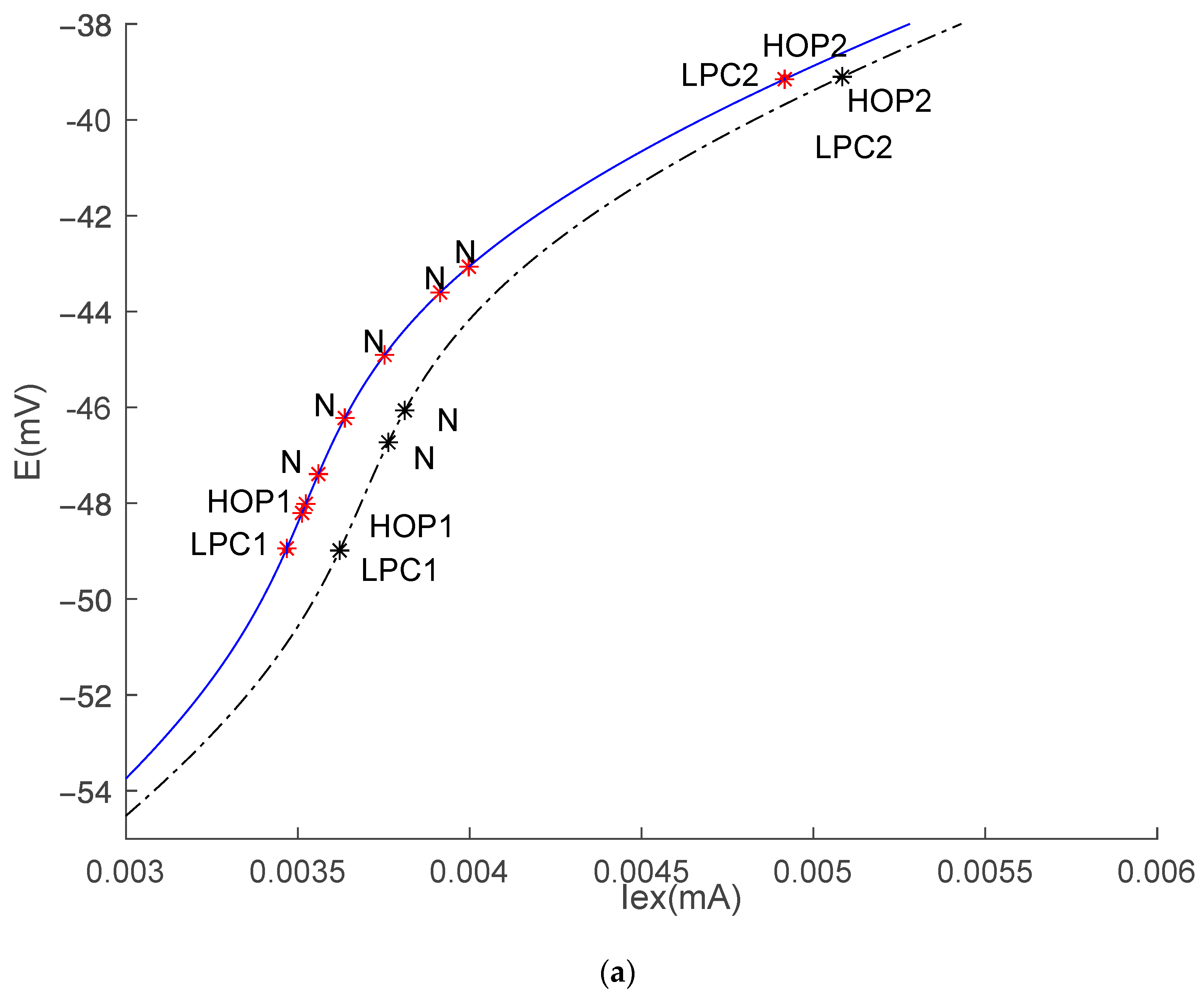
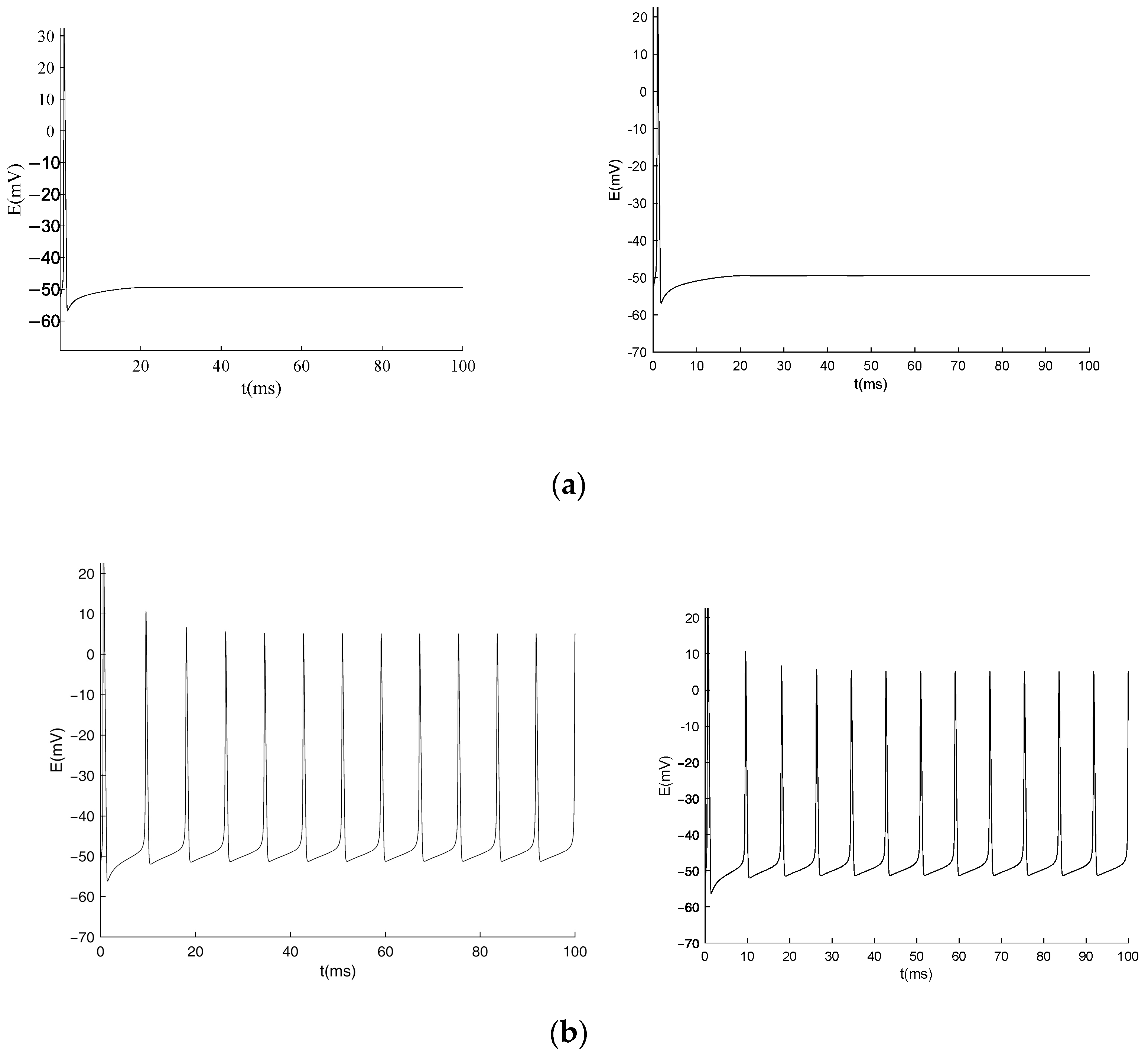
3.1. Equilibrium Point and Stability Analysis of HH Models

By numerically solving the equilibrium point, we can obtain the relationship between the equilibrium potential of the HH models (HH1 and HH2) and the stimulation current I_ex, as shown in Figure 1a. The first Hopf bifurcation (Hop1) occurs at I_ex = 0.0036215315 mA in HH1 and I_ex = 0.0036107258 mA in HH2, and the first Lyapunov coefficient (l₁) of HH1 (l₁ = 0.293) and HH2 (l₁ = 0.275) is positive, which means that the bifurcation point is a subcritical bifurcation point and that unstable limit cycles will generate from it. The second Hopf bifurcation (Hop2) occurs at I_ex = 0.0050838178 mA in HH1 and I_ex = 0.0050715831 mA in HH2, and their first Lyapunov coefficients (l₁ = −0.0558 in HH1 and l₁ = −0.0569 in HH2) are negative, which means that the bifurcation point is a subcritical bifurcation point and that stable limit cycles will generate from it. There are two limit cycle bifurcation points, LPC1 (I_ex = 0.00362 mA in HH1 and I_ex = 0.00361 mA in HH2) and LPC2 (I_ex = 0.00508 mA in HH1 and I_ex = 0.00507 mA in HH2). As shown in Figure 1b, limit cycles appear at Hopf bifurcations (Hop1 and Hop2) in the HH1 model. Figure 1c exhibits that a subcritical Hopf bifurcation Hop1 gives rise to unstable limit cycles with smaller amplitudes for I_ex < I_Hop1, which disappears via collision with another limit cycle with larger amplitudes at LPC1. There is a period doubling point denoted as PD (I_ex = 0.0036189602 mA in HH1 and I_ex = 0.003608894 mA in HH2) which is one of the routes to chaos.

There are two neutral saddle equilibrium points in HH1, which is the same as the HH model describing the muscle cell [20], and five neutral saddle equilibrium points in HH2. The neutral saddle point is not a bifurcation point; it is a special saddle point whose eigenvalues are all real numbers, but one pair of eigenvalues are the opposite of each other. At a neutral saddle point, the trajectory of the system solution has symmetry about some coordinates. Neutral saddle points are generally in the vicinity of the Hop bifurcation and limit points, implying that there are transition points attached at neutral saddle points. The equilibrium points are listed in

Table 3. Equilibrium points of HH1 and HH2.

−	Model	Iex (mA)	E (mV)	First Lyapunov Coefficient
Hop1	HH1	0.0036215335	−48.99	0.293
	HH2	0.0036107258	−48.98	0.275
Hop2	HH1	0.0050838178	−39.10	−0.056
	HH2	0.0050715831	−39.11	−0.056
Neutral Saddle Equilibrium 1	HH1	0.0037633645	−46.73
		0.0038111984	−46.06
	HH2	0.0036760695	−47.93
		0.00373672154	−46.96
		0.0038167752	−45.85
		0.004026353	−43.88
		0.0041198005	−43.24
LPC1	HH1	0.0036189598	0.0036194737	0.0036174701
	HH2	0.0036087739
LPC2	HH1	0.0050838182
	HH2	0.0050715845
PD	HH1	0.0036189602
	HH2	0.003608894

after calculating with the Matcont toolkit, where all curves are computed by the same function that implements a prediction-correction continuation algorithm based on the Moore–Penrose matrix pseudo-inverse [21].

To illustrate the response of the HH model to different current stimuli, we simulated the changes of membrane potentials under three current stimulation intensities (0.0035 mA, 0.0037 mA, and 0.0052 mA). Figure 2a shows that when the stimulation current is less than the current of Hop1, the membrane potential depolarizes and generates a spike and then returns to an equilibrium state. Not to mention the fact that no spikes occur when the current is even less. When the stimulation current is between the currents of HOP1 and HOP2, the cell membrane potential exhibits repetitive discharge and fails to return to an equilibrium state (Figure 2b). When the stimulation current exceeds the current of HOP2, the cell membrane potential begins to discharge repeatedly but quickly stabilizes to a new equilibrium state (Figure 2c). At this time, the membrane potential is significantly higher than the potential in the stable state. Figure 2 shows that the results of HH1 and HH2 are identical.

A neuron is considered as quiescent if its membrane potential is at rest or exhibits only small amplitude oscillations. These two cases correspond to a stable state or to a small amplitude limit cycle attractor, respectively. Excitability occurs when a small perturbation can drive the system from its quiescent state to a large excursion (much larger than the small amplitude perturbation), also called a spike, before returning to its initial quiescent state [7]. Such excitable behavior does occur when the quiescent state is close to a bifurcation that allows the system to visit a large amplitude periodic pseudo-orbit as shown in Figure 2a. When the current is strong enough, the cell starts to fire repeatedly and the system has stable periodic solutions (Figure 2b). The periodic oscillations exist over a rather wide range of I_ex values (I_Hop1 < I_ex < I_Hop2). When the current increases to a higher value, the repeated discharge eventually disappears. After a period of decay and oscillations, the membrane potential finally returns to a new resting state, which is obviously different from the initial resting state. The new resting state is known as “nerve block” in neurobiology, and cells at this state will not be able to generate repetitive discharge under current stimulation, resulting in response failure [22]. Therefore, it is of great significance for clinical diagnosis and treatment to study the conditions for the generation and disappearance of stable periodic solutions in the model.

3.2. Equilibrium Point and Stability Analysis of the GHK Model

The equilibrium points of the GHK model were calculated and are listed in

Table 4. Equilibrium points of the GHK model.

Point Properties	Iex (mA)	E (mV)	First Lyapunov Coefficient
Hop1	0.00054	−64.53	−2.073
Hop2	0.38712	−34.44	−0.013
LP	0.00054	−64.34
LPC	0.38712	1.14
N	0.00049	−63.25
	0.00052	−63.60

. The current of HOP1 (I_ex = 0.00054 mA) is less than that of the HH models, and the current of HOP2 (I_ex = 0.38 mA) is more than that of the HH models. The first Lyapunov coefficients (l₁) of HOP1 and HOP2 are both negative, which means that stable limit cycles will be generated. From Table 4, we can infer that the range of I_ex that induces repetitive discharge in the GHK model is wider than that in the HH models.

To compare the results with the HH models, we simulated the changes in membrane potential under four current stimulation intensities (0.0006 mA, 0.0035 mA, 0.0052 mA, and 0.39 mA). Figure 3a shows that a very small I_ex = 0.0006 mA can induce repetitive discharge, though it takes several centiseconds to accumulate the stimulation effect. Figure 3d shows that the cell membrane potential stabilizes to a higher equilibrium state after discharging repeatedly under a very high I_ex = 0.39 mA.

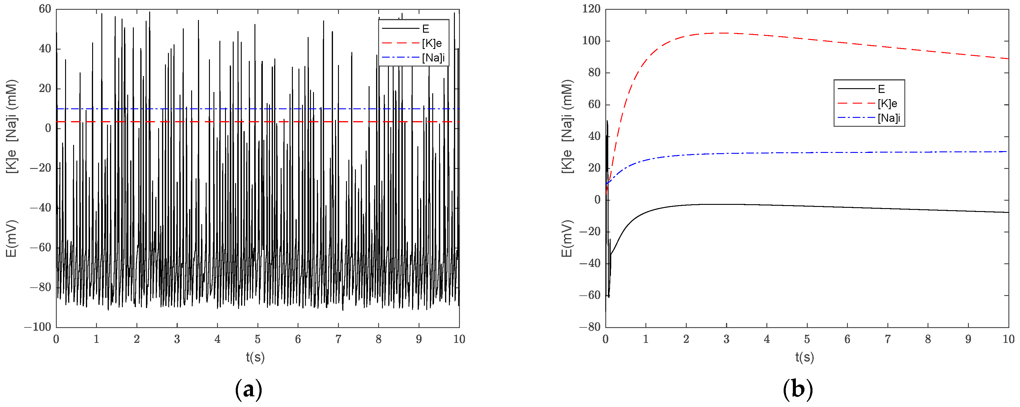
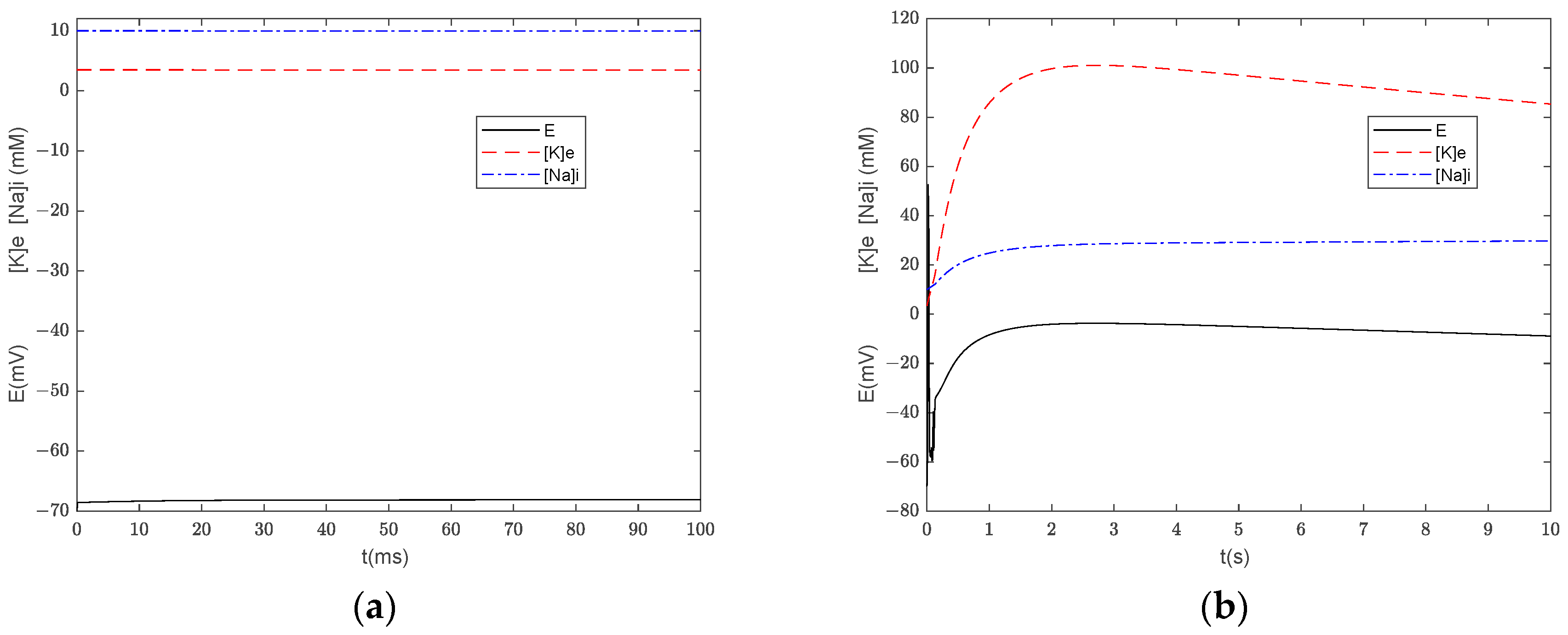
3.3. Numerical Simulation of the Generalized Model

The membrane currents of I_Na and I_K will lead to changes in ion concentration, but it is impossible to obtain the convergent equilibrium solution when considering the actual changes in ion concentration. Therefore, we conducted an analysis on the generalized model without a Na-K pump through numerical simulation. Figure 4a shows that the accumulation of [K]_e makes the action potentials appear about 20 s earlier than that of the GHK model. Figure 4b shows that [K]_e accumulation makes the action potential stabilize to a new equilibrium state more quickly compared with the GHK model (Figure 3d).

Figure 5 compares the numerical results of the GHK model and the generalized model without the Na-K pump. Figure 5a shows the presence of continuous action potential in the GHK model, while Figure 5b shows a short duration of action potential (120 ms), moving from approximately −40 mV to about −10 mV and gradually returning to its resting voltage, resulting in spreading depression (SD)-like depolarization.

The Na+–K+ ATPase pumps 2 K into the cell and therefore contributes to reducing [K]_e. Figure 6 is the simulation results of the generalized model with the Na-K pump. Figure 6a shows that there are no action potentials at I_ex = 0.0006 mA, which is different from those of the GHK mode and the generalized model without the Na-K pump. Figure 6b shows that the SD-like depolarization recovers a little more quickly in the generalized model with the Na-K pump compared with the generalized model without the Na-K pump. The maximum [K]_e is 105 mM in the generalized model without the Na-K pump, while it is 101 mM in the generalized model with the Na-K pump. in the generalized model without the Na-K pump, [K]_e at 10 s is 88.9 mM, while in the generalized model with the Na-K pump, it is 85.4 mM.

4. Discussion and Conclusions

In this paper, we established a generalized model of a specific neuron and its simplified HH models. The dynamic analysis shows that the main channel currents ($I_{\mathrm{Na},\mathrm{T}}$, $I_{\mathrm{K},\mathrm{DR}}$, and $I_{\mathrm{L}}$) of a neuron determine its dynamic properties. The addition of more channel membrane currents ($I_{\mathrm{Na},\mathrm{P}}$ and $I_{\mathrm{K},\mathrm{A}}$) only slightly affects the position of the bifurcation points. The analysis of the dynamic equation shows that the addition of new channels increases the eigenvalues of the equilibrium equation, which are saddle points and have no effect on the bifurcation of the model. Replacing the channel current equation with the GHK formula from the HH equation will considerably broaden the range of stimulation current that gives rise to the action potential. The GHK formula is based on the dynamic description of the membrane current and a nonlinear equation, which leads to greater channel currents. It should be noted that the parameters and values are derived from a GHK model, and the membrane current calculated by the Nernst equation is less than the physiological current simulated by the GHK formula; therefore, the depolarization in the HH model shown in Figure 2b does not reach the physiological level of 35 mV.

Because there is no convergent equilibrium solution in the generalized model, we analyzed its dynamic properties through numerical simulation. Figure 3 and Figure 4 show that the membrane potential in the GHK model and the generalized model are similar at the onset of current stimulation. Figure 5 shows when the current stimulation lasts for a long period of time, the action potential in the GHK model persists, while SD-like depolarization occurs in the generalized model. Figure 5b shows that the trends of changes in [K]_e and E are consistent in the generalized model. [K]_e is a factor that induces SD-like depolarization, which is another topic in neuron analysis [23,24]. As for current stimulation, [K]_e stimulation will also induce action potential; this paper does not discuss this because the ion concentration stays constant in HH models. The result of the numerical analysis shows that HH models are suitable for describing the response to an initial stimulation, when the change in [K]_e is too small to infect the response; if studying the response to a long stimulation, the change in ion concentration must be included, and thus the generalized model is suitable, and the numerical oscillation analysis diagrams can be used to analyze the limit cycles [25]. Figure 6 shows that the inclusion of the Na-K pump will weaken the current stimulation effect by decreasing [K]_e accumulation. More current stimulation is needed to induce action potential, and E recovers to the rest state more quickly.

The human nervous system consists of thousands of millions of neurons, and efficient communication among them is critical for the correct function of the central nervous system [26]. It is important not only for life sciences, but also for the development of medicine, artificial intelligence, computer science, control science, and information science. For example, the opportunities for smart applications have increased dramatically as billions of devices are connected via the Internet [27], and the usefulness of chaotic neurons for secure image transmission is one aspect [6]. The echo state network (ESN) is one of the most used machine learning methods for predicting chaotic time, and González-Zapata et al. analyzed different ESN topologies by modifying the structure and number of internal connections in the hidden layer, in which neurons are connected randomly [28].

It should be noted that all five models in this paper are based on the HH model; the GHK model is a nonlinear GHK current instead of the linear Nernst current in the HH model, and the generalized model includes the variation in the ion concentration. Though there are many types of neuron models, the HH model still dominates the field, and many models have been proposed on the basis of corrections to the HH model, and the HH model applies not only to nerve cells but also to other excitable cells. For example, it is also widely used in other excitable cells, such as muscle cells.

References

1. Lu, Y.; Xin, X.; Rinzel, J. Bistability at the onset of neuronal oscillations. Biol. Cybern. 2023, 117, 61–79. [Google Scholar] [CrossRef]
2. Noble, D. How the Hodgkin cycle became the principle of biological relativity. J. Physiol. 2022, 600, 5171–5177. [Google Scholar] [CrossRef]
3. FitzHugh, R. Impulses and Physiological States in Theoretical Models of Nerve Membrane. Biophys. J. 1961, 1, 445–466. [Google Scholar] [CrossRef]
4. Morris, C.; Lecar, H. Voltage oscillations in the barnacle giant muscle fiber. Biophys. J. 1981, 35, 193–213. [Google Scholar] [CrossRef]
5. Hindmarsh, J.L.; Rose, R.M. A model of the nerve impulse using two first-order differential equations. Nature 1982, 296, 162–164. [Google Scholar] [CrossRef]
6. González-Zapata, A.M.; Tlelo-Cuautle, E.; Cruz-Vega, I.; León-Salas, W.D. Synchronization of chaotic artificial neurons and its application to secure image transmission under MQTT for IoT protocol. Nonlinear Dyn. 2021, 104, 4581–4600. [Google Scholar] [CrossRef]
7. Izhikevich, E.M. Neural excitability, spiking and bursting. Int. J. Bifurc. Chaos 2000, 6, 1171–1266. [Google Scholar] [CrossRef]
8. Tóth, K.; Okun, M. Seventy years later: The legacy of the Hodgkin and Huxley model in computational neuroscience. J. Physiol. 2023, 601, 3009–3010. [Google Scholar] [CrossRef]
9. Cooley, J.; Dodge, F.; Cohen, H. Digital computer solutions for excitable membrane models. J. Cell Comp. Physiol. 1965, 66, 99–109. [Google Scholar] [CrossRef]
10. Rinzel, J. Repetitive activity in nerve. Fed. Proc. 1978, 37, 2793–2802. [Google Scholar]
11. Aihara, K.; Matsumoto, G. Two stable steady states in the Hodgkin-Huxley axons. Biophys. J. 1983, 41, 87–89. [Google Scholar] [CrossRef]
12. Rabinovich, M.I.; Varona, P.; Selverston, A.I.; Abarbanel, H.D.I. Dynamical principles in neuroscience. Rev. Mod. Phys. 2006, 78, 1213–1265. [Google Scholar] [CrossRef]
13. Che, Y.; Wang, J.; Deng, B.; Wei, X.; Han, C. Bifurcations in the Hodgkin–Huxley model exposed to DC electric fields. Neurocomputing 2012, 81, 41–48. [Google Scholar] [CrossRef]
14. Guckenheimer, J.; Labouriau, J.S. Bifurcation of the Hodgkin and Huxley equations: A new twist. Bull. Math. Biol. 1993, 55, 937–952. [Google Scholar] [CrossRef]
15. Fukai, H.; Nomura, T.; Doi, S.; Sato, S. Hopf bifurcations in multiple-parameter space of the Hodgkin-Huxley equations II. Singularity theoretic approach and highly degenerate bifurcations. Biol. Cybern. 2000, 82, 223–229. [Google Scholar] [CrossRef]
16. Fukai, H.; Doi, S.; Nomura, T.; Sato, S. Hopf bifurcations in multiple-parameter space of the Hodgkin-Huxley equations I. Global organization of bistable periodic solutions. Biol. Cybern. 2000, 82, 215–222. [Google Scholar] [CrossRef]
17. Yao, W.; Li, Y.; Ou, Z.; Sun, M.; Ma, Q.; Ding, G. Dynamic analysis of neural signal based on Hodgkin–Huxley model. Math. Methods Appl. Sci. 2022, 46, 4676–4687. [Google Scholar] [CrossRef]
18. James Keener, J.S. Mathematical Physiology, 2nd ed.; Springer: New York, NY, USA, 2008. [Google Scholar]
19. Yao, W.; Huang, H.; Miura, R.M. A Continuum Neuronal Model for the Instigation and Propagation of Cortical Spreading Depression. Bull. Math. Biol. 2011, 73, 2773–2790. [Google Scholar] [CrossRef]
20. Ma, Q.X.; Arneodo, A.; Ding, G.H.; Argoul, F. Dynamical study of Nav channel excitability under mechanical stress. Biol. Cybern. 2017, 111, 129–148. [Google Scholar] [CrossRef]
21. Dhooge, A.; Govaerts, W.; Kuznetsov, Y.A. MATCONT: A Matlab Package for Numerical Bifurcation Analysis of ODEs. ACM Trans. Math. Softw. (TOMS) 2003, 29, 141–164. [Google Scholar] [CrossRef]
22. Rinzel, J.; Huguet, G. Nonlinear Dynamics of Neuronal Excitability, Oscillations, and Coincidence Detection. Commun. Pure Appl. Math. 2013, 66, 1464–1494. [Google Scholar] [CrossRef] [PubMed]
23. Kager, H.; Wadman, W.J.; Somjen, G.G. Simulated Seizures and Spreading Depression in a Neuron Model Incorporating Interstitial Space and Ion Concentrations. J. Neurophysiol. 2000, 84, 495–512. [Google Scholar] [CrossRef] [PubMed]
24. Müller, M.; Somjen, G.G. Na and K Concentrations, Extra- and Intracellular Voltages, and the Effect of TTX in Hypoxic Rat Hippocampal Slices. J. Neurophysiol. 2000, 83, 735–745. [Google Scholar] [CrossRef] [PubMed]
25. Sun, M.; Li, Y.; Yao, W. A Dynamic Model of Cytosolic Calcium Concentration Oscillations in Mast Cells. Mathematics 2021, 9, 2322. [Google Scholar] [CrossRef]
26. Yao, W.; Huang, H.; Miura, R.M. Role of Astrocyte in Cortical Spreading Depression: A Quantitative Model of Neuron-Astrocyte Network. Commun. Comput. Phys. 2018, 23, 440–458. [Google Scholar] [CrossRef]
27. Strous, L.; von Solms, S.; Zúquete, A. Security and privacy of the Internet of Things. Comput. Secur. 2021, 102, 102148. [Google Scholar] [CrossRef]
28. Gonzalez-Zapata, A.M.; de la Fraga, L.G.; Ovilla-Martinez, B.; Tlelo-Cuautle, E.; Cruz-Vega, I. Enhanced FPGA implementation of Echo State Networks for chaotic time series prediction. Integration 2023, 92, 48–57. [Google Scholar] [CrossRef]
Figure 1. Stability analysis of the HH models. (a) Equilibrium points in HH1 and HH2; the blue line represents HH2, and the black dashed line represents HH1. (b) Limit cycles of HH1. (c) Zoomed-in image (b).
Appliedmath 03 00041 g001aAppliedmath 03 00041 g001b
Figure 2. Simulation results of membrane potentials under different stimulation currents. The left column is the result of HH1; the right column is the result of HH2. (a) under Iex = 0.0035 mA, (b) under Iex = 0.0037 mA, and (c) under Iex = 0.0052 mA.
Appliedmath 03 00041 g002aAppliedmath 03 00041 g002b
Figure 3. Simulation results of membrane potentials under the different stimulation currents of the GHK model. (a) under Iex = 0.0006 mA, (b) under Iex = 0.0035 mA, (c) under Iex = 0.0052 mA, (d) and under Iex = 0.39 mA.
Appliedmath 03 00041 g003
Figure 4. Simulation result of membrane potentials (E), intracellular Na concentration ([Na]i), and extracellular K concentration ([K]e) under the different stimulation currents of the generalized model without a Na-K pump. (a) under Iex = 0.0006 mA and (b) under Iex = 0.39 mA.
Appliedmath 03 00041 g004
Figure 5. Simulation result of E, [Na]I, and [K]e under Iex = 0.0052 mA of the different model. (a) GHK model A, and (b) the generalized model without a Na-K pump.
Appliedmath 03 00041 g005
Figure 6. Simulation results of E, [Na]i, and [K]e under the different currents of the generalized model with a Na-K pump. (a) under Iex = 0.0006 mA and (b) under Iex = 0.0052 mA.
Appliedmath 03 00041 g006