
Local Normal Approximations and Probability Metric Bounds for the Matrix-Variate T Distribution and Its Application to Hotelling’s T Statistic


Abstract
1. Introduction
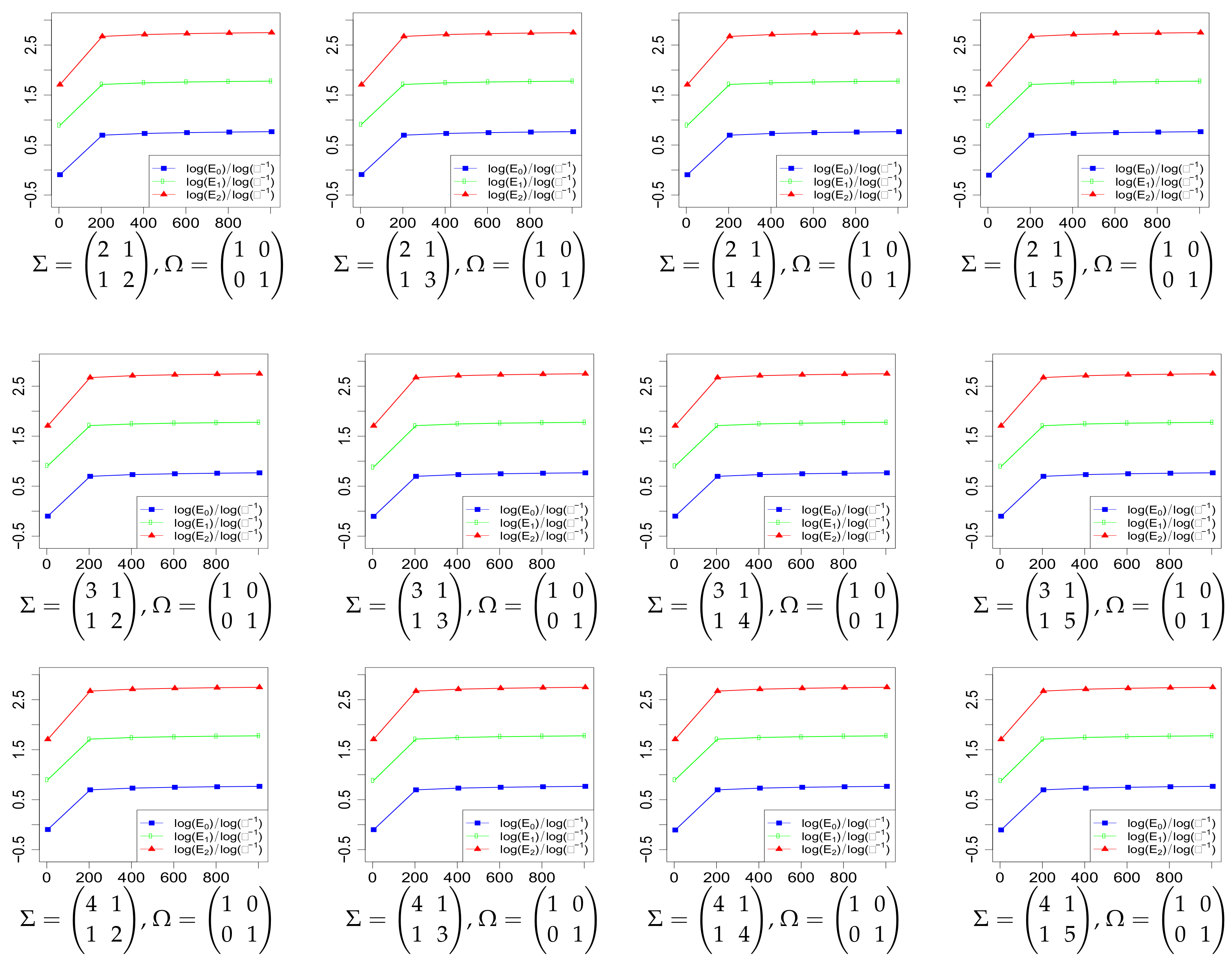
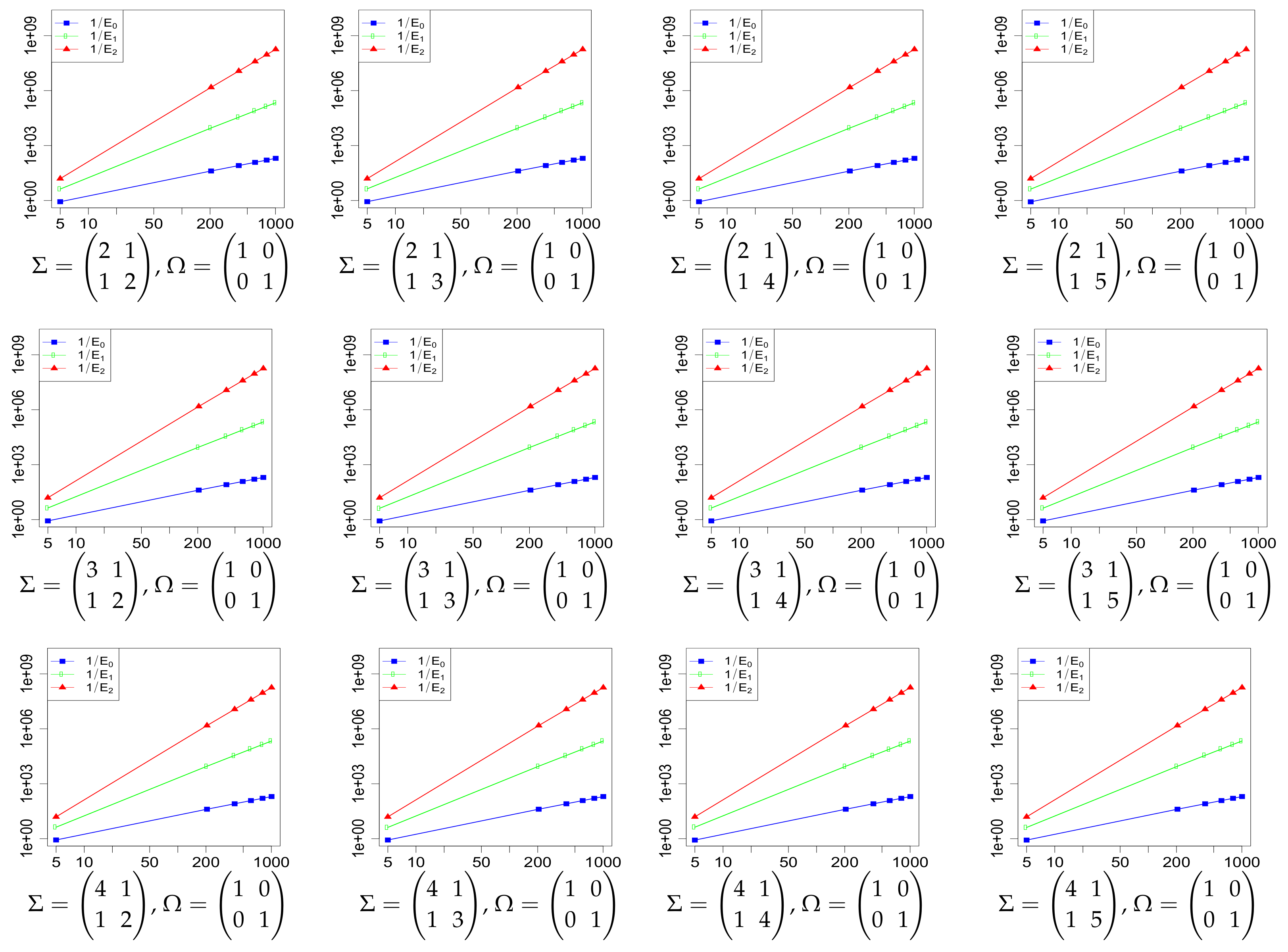
2. Main Results
3. Proofs
Supplementary Materials
Funding
Institutional Review Board Statement
Informed Consent Statement
Data Availability Statement
Acknowledgments
Conflicts of Interest
Appendix A. Technical Computations
References
- Gupta, A.K.; Nagar, D.K. Matrix Variate Distributions, 1st ed.; Chapman and Hall/CRC: Boca Raton, FL, USA, 1999; p. 384. [Google Scholar]
- Olver, F.W.J.; Lozier, D.W.; Boisvert, R.F.; Clark, C.W. (Eds.) NIST Handbook of Mathematical Functions; U.S. Department of Commerce, National Institute of Standards and Technology: Washington, DC, USA; Cambridge University Press: Cambridge, UK, 2010; p. xvi+951. [Google Scholar]
- Nagar, D.K.; Roldán-Correa, A.; Gupta, A.K. Extended matrix variate gamma and beta functions. J. Multivar. Anal. 2013, 122, 53–69. [Google Scholar] [CrossRef]
- Pajevic, S.; Basser, P.J. Parametric description of noise in diffusion tensor MRI. In Proceedings of the 7th Annual Meeting of the ISMRM, Philadelphia, PA, USA, 22–28 May 1999; p. 1787. [Google Scholar]
- Basser, P.J.; Jones, D.K. Diffusion-tensor MRI: Theory, experimental design and data analysis—A technical review. NMR Biomed. 2002, 15, 456–467. [Google Scholar] [CrossRef] [PubMed]
- Pajevic, S.; Basser, P.J. Parametric and non-parametric statistical analysis of DT-MRI data. J. Magn. Reson. 2003, 161, 1–14. [Google Scholar] [CrossRef]
- Basser, P.J.; Pajevic, S. A normal distribution for tensor-valued random variables: Applications to diffusion tensor MRI. IEEE Trans. Med. Imaging 2003, 22, 785–794. [Google Scholar] [CrossRef] [PubMed]
- Gasbarra, D.; Pajevic, S.; Basser, P.J. Eigenvalues of random matrices with isotropic Gaussian noise and the design of diffusion tensor imaging experiments. SIAM J. Imaging Sci. 2017, 10, 1511–1548. [Google Scholar] [CrossRef] [PubMed][Green Version]
- Alexander, D.C.; Pierpaoli, C.; Basser, P.J.; Gee, J.C. Spatial transformations of diffusion tensor magnetic resonance images. IEEE Trans. Med. Imaging 2001, 20, 1131–1139. [Google Scholar] [CrossRef] [PubMed]
- Schwartzman, A.; Mascarenhas, W.F.; Taylor, J.E. Inference for eigenvalues and eigenvectors of Gaussian symmetric matrices. Ann. Statist. 2008, 36, 2886–2919. [Google Scholar] [CrossRef]
- Mallows, C.L. Latent vectors of random symmetric matrices. Biometrika 1961, 48, 133–149. [Google Scholar] [CrossRef]
- Hu, W.; White, M. A CMB polarization primer. New Astron. 1997, 2, 323–344. [Google Scholar] [CrossRef]
- Vafaei Sadr, A.; Movahed, S.M.S. Clustering of local extrema in Planck CMB maps. MNRAS 2021, 503, 815–829. [Google Scholar] [CrossRef]
- Gallaugher, M.P.B.; McNicholas, P.D. Finite mixtures of skewed matrix variate distributions. Pattern Recognit. 2018, 80, 83–93. [Google Scholar] [CrossRef]
- Ouimet, F. Refined normal approximations for the Student distribution. J. Classical Anal. 2022, 20, 23–33. [Google Scholar] [CrossRef]
- Shafiei, A.; Saberali, S.M. A simple asymptotic bound on the error of the ordinary normal approximation to the Student’s t-distribution. IEEE Commun. Lett. 2015, 19, 1295–1298. [Google Scholar] [CrossRef]
- Govindarajulu, Z. Normal approximations to the classical discrete distributions. Sankhyā Ser. A 1965, 27, 143–172. [Google Scholar]
- Esseen, C.G. Fourier analysis of distribution functions. A mathematical study of the Laplace-Gaussian law. Acta Math. 1945, 77, 1–125. [Google Scholar] [CrossRef]
- Cressie, N. A finely tuned continuity correction. Ann. Inst. Statist. Math. 1978, 30, 435–442. [Google Scholar] [CrossRef]
- Gaunt, R.E. Variance-gamma approximation via Stein’s method. Electron. J. Probab. 2014, 19, 1–33. [Google Scholar] [CrossRef]
- Gaunt, R.E. New error bounds for Laplace approximation via Stein’s method. ESAIM Probab. Stat. 2021, 25, 325–345. [Google Scholar] [CrossRef]
- Gaunt, R.E. Wasserstein and Kolmogorov error bounds for variance-gamma approximation via Stein’s method I. J. Theoret. Probab. 2020, 33, 465–505. [Google Scholar] [CrossRef]
- R Core Team. R: A Language and Environment for Statistical Computing; R Foundation for Statistical Computing: Vienna, Austria, 2020. [Google Scholar]
- Hotelling, H. The generalization of Student’s ratio. Ann. Math. Statist. 1931, 2, 360–378. [Google Scholar] [CrossRef]
- Abramowitz, M.; Stegun, I.A. Handbook of Mathematical Functions with Formulas, Graphs, and Mathematical Tables; National Bureau of Standards Applied Mathematics Series, For sale by the Superintendent of Documents; U.S. Government Printing Office: Washington, DC, USA, 1964; Volume 55, p. xiv+1046. [Google Scholar]
- Carter, A.V. Deficiency distance between multinomial and multivariate normal experiments. Ann. Statist. 2002, 30, 708–730. [Google Scholar] [CrossRef]
- de Waal, D.J.; Nel, D.G. On some expectations with respect to Wishart matrices. South African Statist. J. 1973, 7, 61–67. [Google Scholar]
- Letac, G.; Massam, H. All invariant moments of the Wishart distribution. Scand. J. Statist. 2004, 31, 295–318. [Google Scholar] [CrossRef]
- Haff, L.R. An identity for the Wishart distribution with applications. J. Multivar. Anal. 1979, 9, 531–544. [Google Scholar] [CrossRef]
- von Rosen, D. Moments for the inverted Wishart distribution. Scand. J. Statist. 1988, 15, 97–109. [Google Scholar] [CrossRef]


Publisher’s Note: MDPI stays neutral with regard to jurisdictional claims in published maps and institutional affiliations. |
© 2022 by the author. Licensee MDPI, Basel, Switzerland. This article is an open access article distributed under the terms and conditions of the Creative Commons Attribution (CC BY) license (https://creativecommons.org/licenses/by/4.0/).
Share and Cite
Ouimet, F. Local Normal Approximations and Probability Metric Bounds for the Matrix-Variate T Distribution and Its Application to Hotelling’s T Statistic. AppliedMath 2022, 2, 446-456. https://doi.org/10.3390/appliedmath2030025
Ouimet F. Local Normal Approximations and Probability Metric Bounds for the Matrix-Variate T Distribution and Its Application to Hotelling’s T Statistic. AppliedMath. 2022; 2(3):446-456. https://doi.org/10.3390/appliedmath2030025
Chicago/Turabian StyleOuimet, Frédéric. 2022. "Local Normal Approximations and Probability Metric Bounds for the Matrix-Variate T Distribution and Its Application to Hotelling’s T Statistic" AppliedMath 2, no. 3: 446-456. https://doi.org/10.3390/appliedmath2030025
APA StyleOuimet, F. (2022). Local Normal Approximations and Probability Metric Bounds for the Matrix-Variate T Distribution and Its Application to Hotelling’s T Statistic. AppliedMath, 2(3), 446-456. https://doi.org/10.3390/appliedmath2030025