Individual Variation in Diet of Four Fishes in Shallow Tropical Estuarine Areas: Comparisons Between Seasons and Habitats


Abstract
1. Introduction
2. Materials and Methods
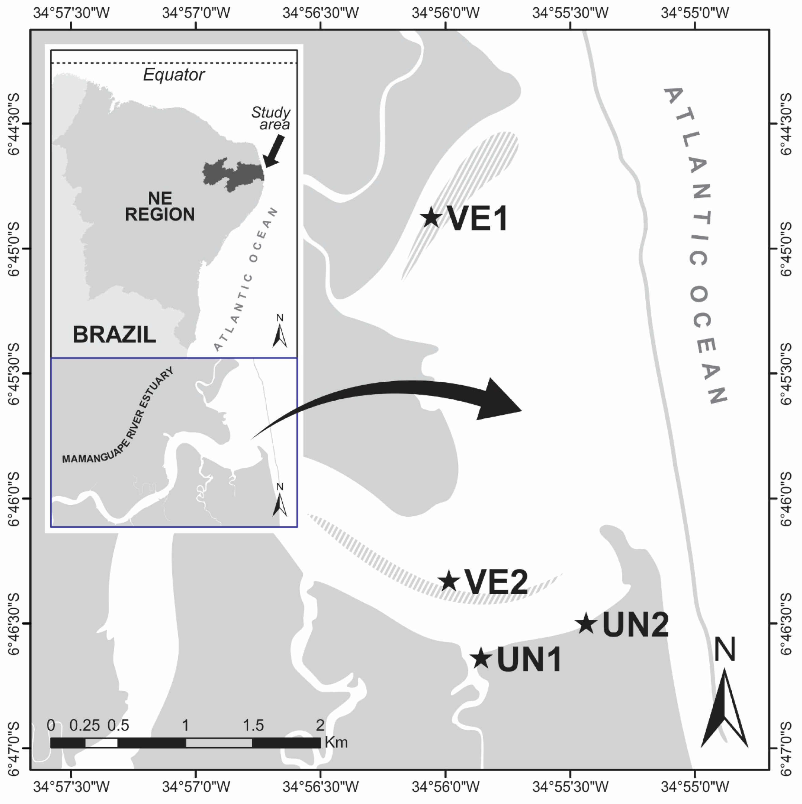
2.1. Study Area
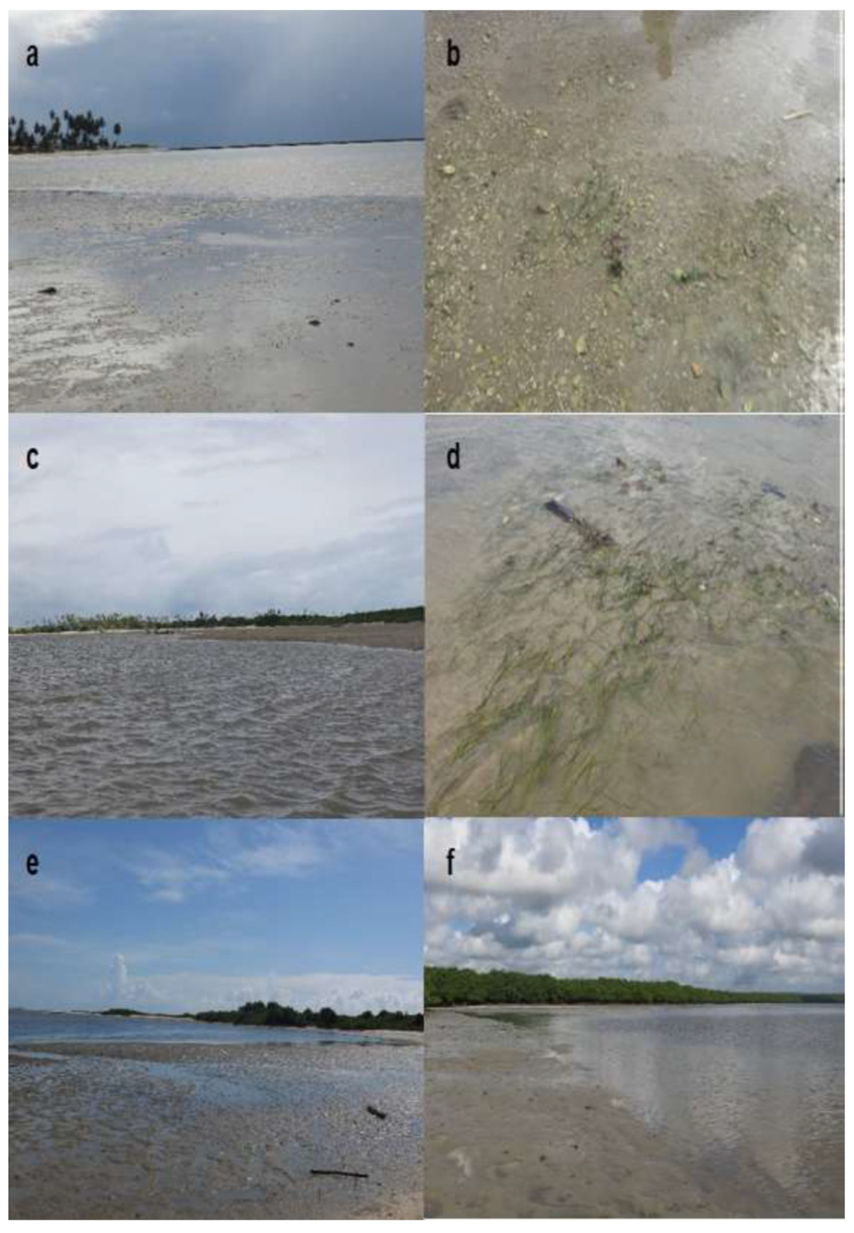
2.2. Sampling and Dietary Analysis
2.3. Size Structure
2.4. Statistical Analysis
3. Results
3.1. Spatial and Temporal Distribution
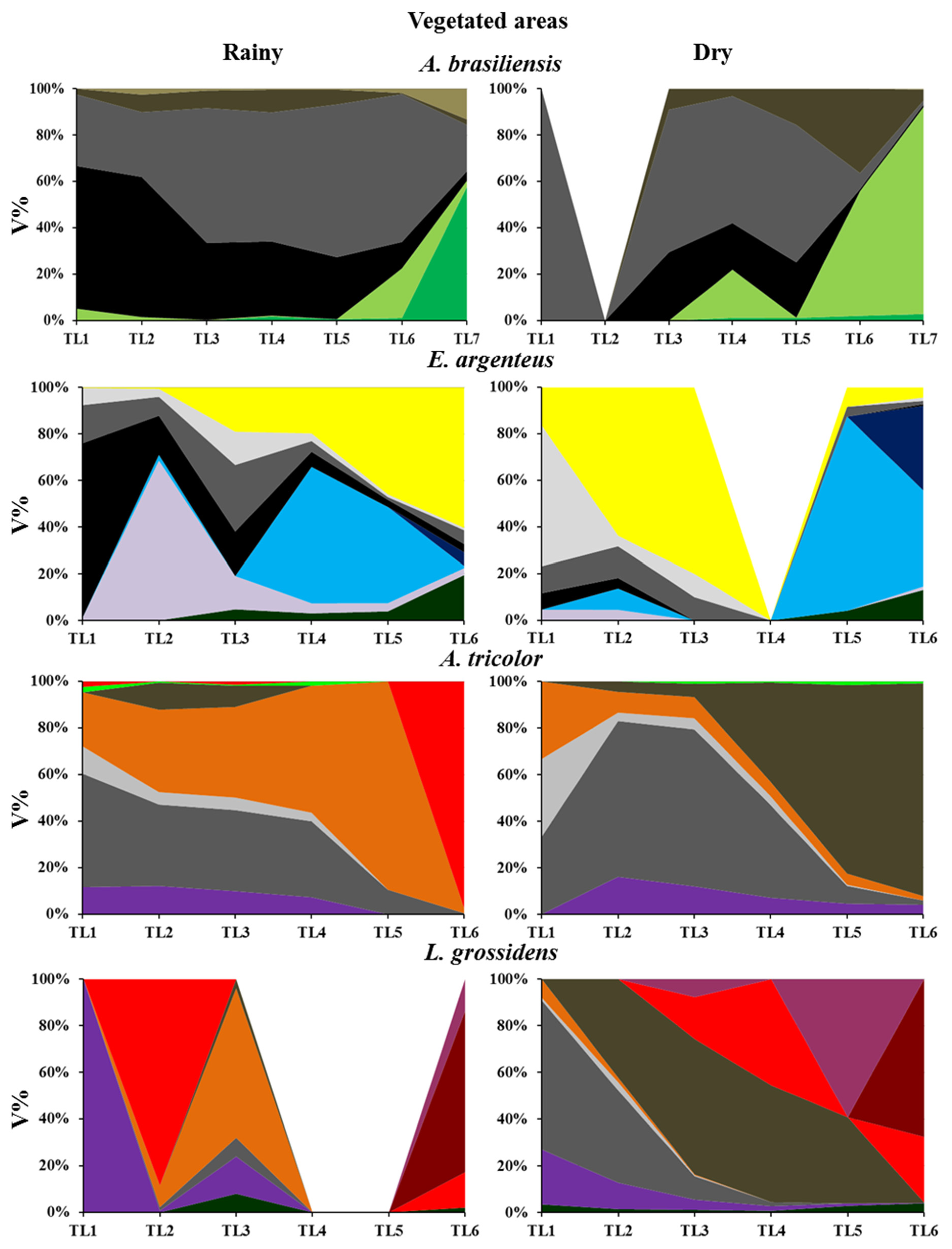
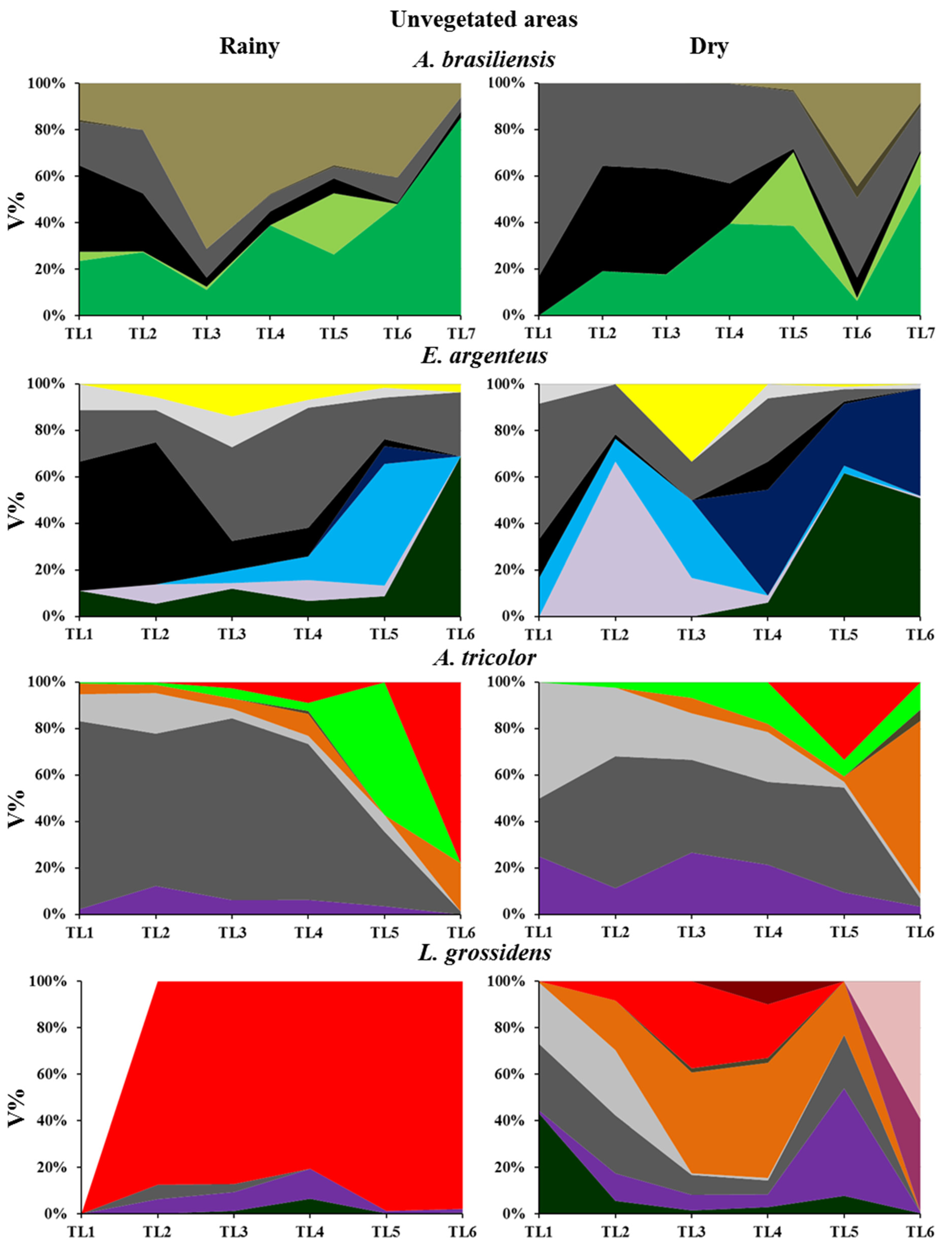
3.2. Diet Composition
4. Ontogenetic Shifts
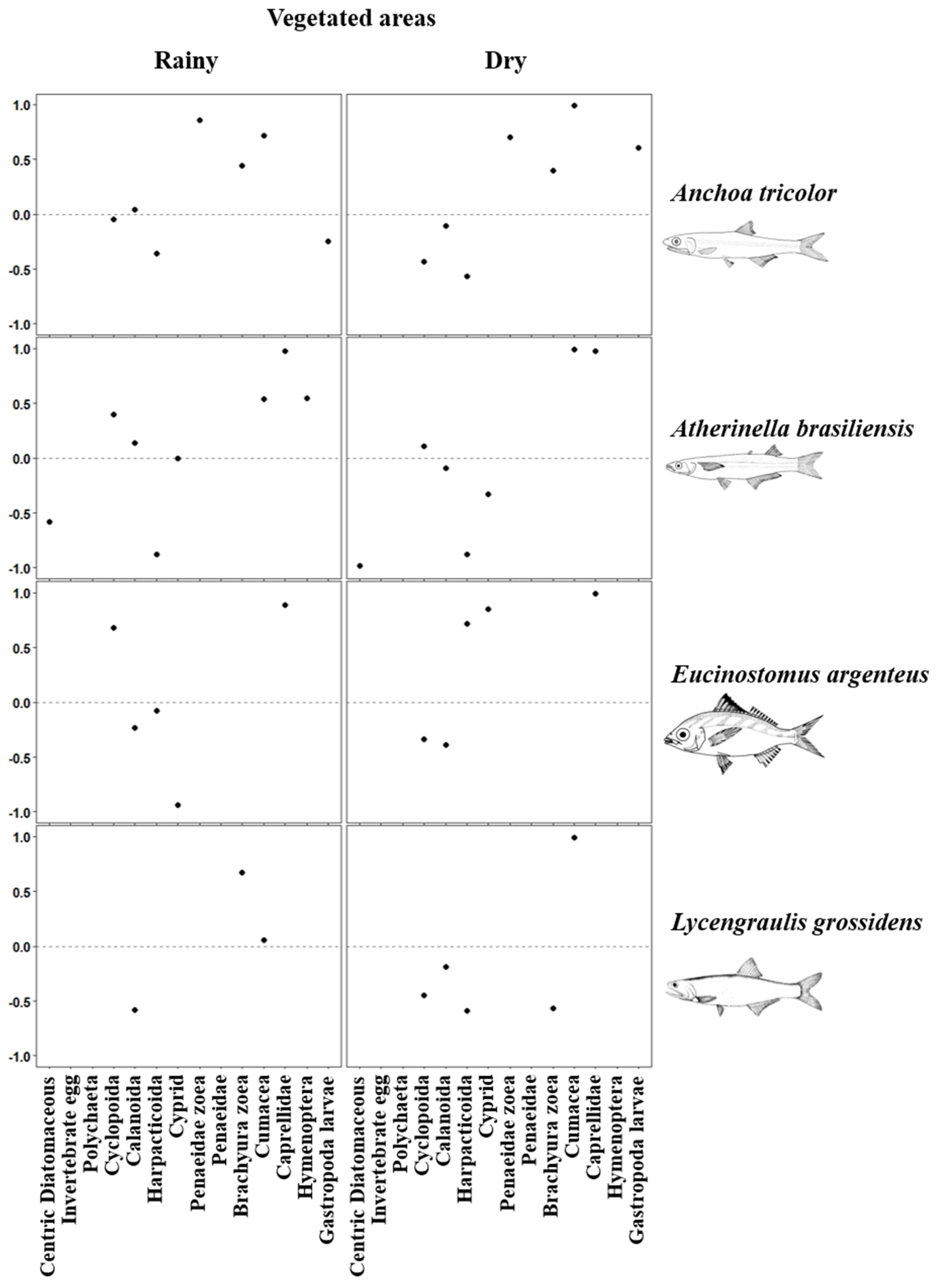
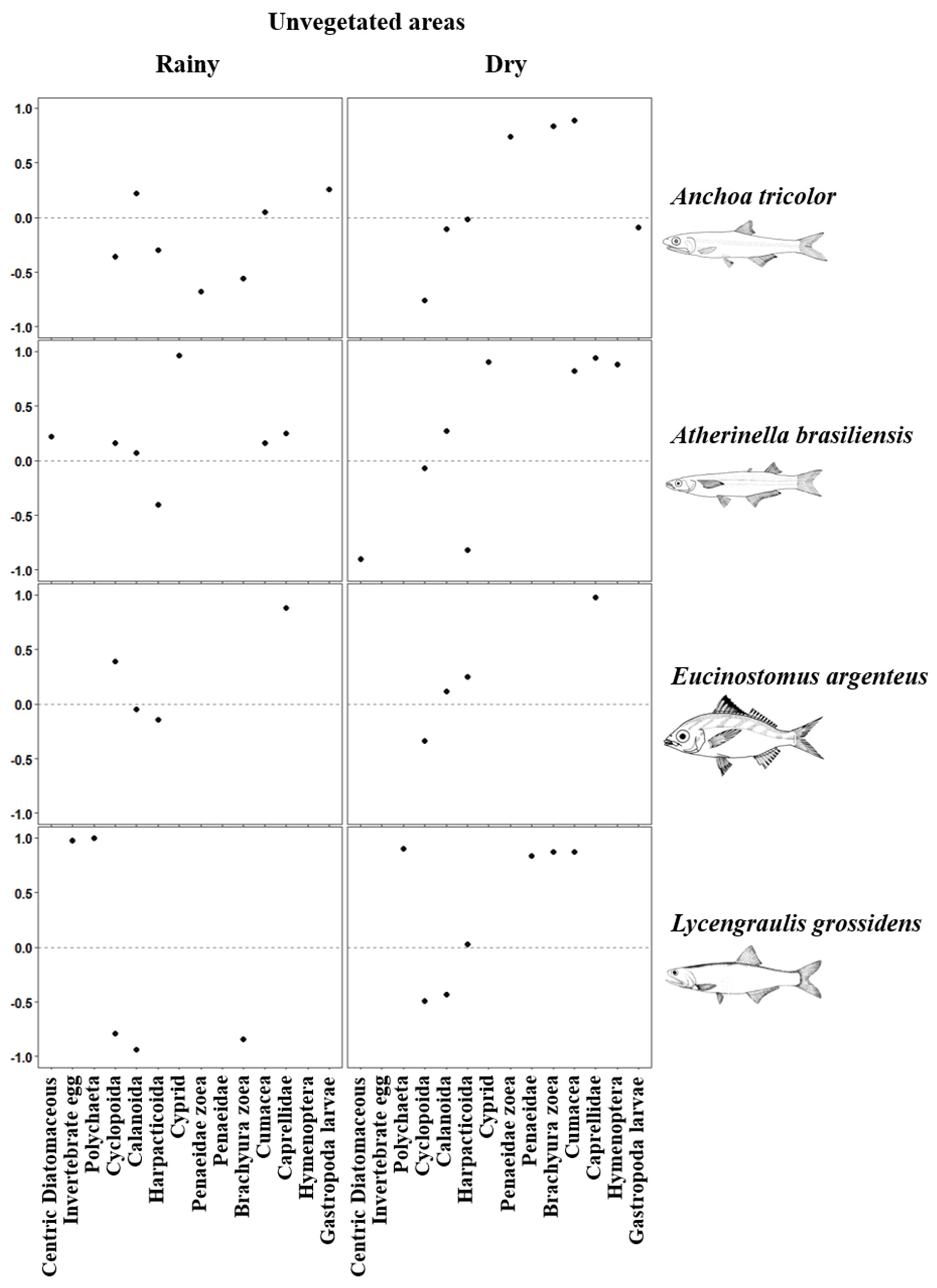
4.1. Feeding Selectivity

| Vegetated Areas | Unvegetated Areas | |||
|---|---|---|---|---|
| Prey (Abbreviation) | Rainy | Dry | Rainy | Dry |
| Foraminifera (FRM) | 0.24 | 0.77 | 0.04 | 0.02 |
| Diatomaceous (DIA) | 5.93 | 1.34 | 5.52 | 9.80 |
| Centric diatomaceous (DCE) | 2.34 | 0.71 | 1.63 | 0.79 |
| Pennate diatomaceous (DPE) | - | - | - | 0.30 |
| Invertebrate egg (EIN) | 0.03 | 0.17 | 0.14 | - |
| Nematoda (NEM) | 0.13 | - | - | 0.03 |
| Polychaeta Larvae (LPO) | 0.68 | 0.37 | 0.02 | 0.02 |
| Polychaeta (POL) | 0.05 | 0.01 | 0.01 | 0.01 |
| Cyclopoida (CYC) | 10.31 | 9.96 | 15.22 | 17.89 |
| Calanoida (CAL) | 42.56 | 67.25 | 45.09 | 43.18 |
| Harpacticoida (HAR) | 15.87 | 6.48 | 14.17 | 11.00 |
| Cyprid (CYP) | 0.26 | 0.26 | 0.15 | 0.06 |
| Nauplius (NAU) | 5.71 | 5.61 | 2.21 | 7.81 |
| Penaeidae zoea (ZPE) | 0.21 | 0.03 | 0.34 | 0.06 |
| Penaeidae (PEN) | - | - | - | 0.01 |
| Brachyuran zoea (ZBR) | 11.49 | 3.43 | 12.58 | 3.34 |
| Brachyuran antizoea (ABR) | - | - | - | 0.02 |
| Brachyuran megalopa (MBR) | - | - | - | 0.01 |
| Porcellanidae zoea (ZPO) | - | - | - | 0.05 |
| Mysis (MYS) | 0.09 | 0.03 | 0.05 | 0.07 |
| Mysida (MYA) | 0.07 | 0.28 | 0.26 | 0.29 |
| Cumacea (CUM) | 0.38 | 0.07 | 0.06 | 0.03 |
| Isopoda (ISO) | 0.07 | - | 0.01 | - |
| Gammaridae (GAM) | 0.05 | 0.08 | 0.01 | - |
| Caprellidae (CAP) | 0.10 | 0.06 | 0.15 | 0.02 |
| Amphipoda (AMP) | 0.30 | 0.62 | 0.09 | 0.02 |
| Ostracoda (OST) | 0.21 | 0.51 | 0.07 | 0.04 |
| Ceratopogonidae larvae (LCE) | 0.02 | - | - | 0.01 |
| Ceratopogonidae pupa (PCE) | 0.02 | - | - | - |
| Diptera (DIP) | - | - | - | 0.02 |
| Hymenoptera (HYM) | 0.02 | - | - | 0.01 |
| Gastropoda larvae (LGA) | 0.14 | 0.31 | 0.79 | 4.60 |
| Bivalvia larvae (LBI) | - | - | 0.19 | 0.02 |
| Lophophorata (LOF) | 0.21 | 0.03 | 0.08 | - |
| Chaetognatha (CHA) | 0.44 | 0.27 | 0.72 | 0.08 |
| Fish eggs (EFI) | 1.11 | 0.27 | 0.07 | 0.30 |
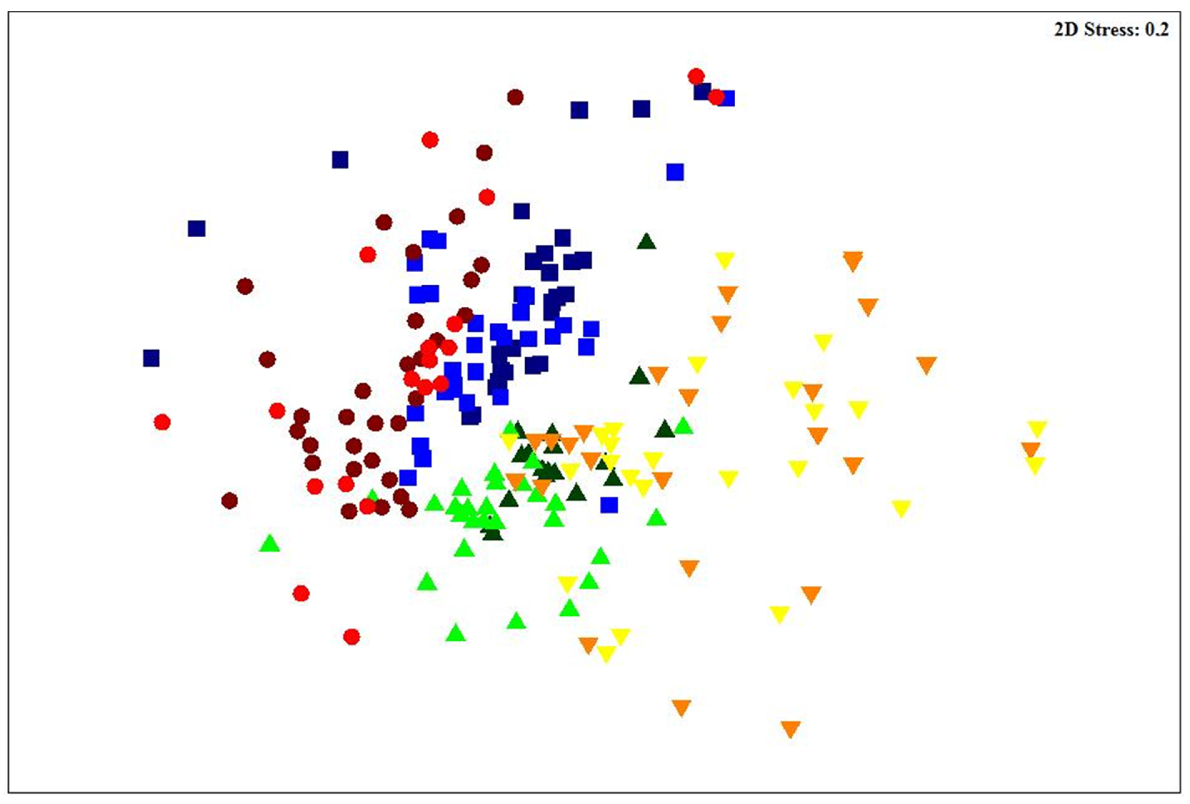
4.2. Individual Specialization
4.3. Niche Breadth and Dietary Overlap
5. Discussion
Author Contributions
Funding
Data Availability Statement
Conflicts of Interest
Appendix A
Appendix A.1

Appendix A.2
| Atherinella brasiliensis | ||||||||||||||||||||||||||||
|---|---|---|---|---|---|---|---|---|---|---|---|---|---|---|---|---|---|---|---|---|---|---|---|---|---|---|---|---|
| Vegetated Areas | ||||||||||||||||||||||||||||
| Rainy | Dry | |||||||||||||||||||||||||||
| TL1 (12) | TL2 (23) | TL3 (33) | TL4 (32) | TL5 (28) | TL6 (39) | TL7 (60) | TL1 (1) | TL2 (0) | TL3 (4) | TL4 (16) | TL5 (14) | TL6 (37) | TL7 (40) | |||||||||||||||
| Items | N% | V% | N% | V% | N% | V% | N% | V% | N% | V% | N% | V% | N% | V% | N% | V% | N% | V% | N% | V% | N% | V% | N% | V% | N% | V% | N% | V% |
| Algae | - | - | - | - | - | - | 0.07 | 0.30 | <0.01 | 0.15 | 0.04 | 0.12 | 0.06 | 3.42 | - | - | - | - | - | - | <0.01 | 0.52 | 0.01 | 0.26 | 0.03 | 0.99 | 0.11 | 1.10 |
| Plant material | 0.01 | 0.63 | 0.02 | 0.80 | 0.02 | 1.06 | 0.04 | 2.27 | 0.01 | 1.34 | 0.06 | 5.38 | 0.12 | 3.57 | - | - | - | - | 0.02 | 1.95 | 0.04 | 3.09 | 0.06 | 3.44 | 0.07 | 2.73 | 0.22 | 3.20 |
| Foraminifera | - | - | 0.17 | 0.20 | 0.10 | 0.18 | 0.17 | 0.23 | 0.12 | 0.15 | 0.03 | 0.03 | 0.28 | 0.06 | - | - | - | - | - | - | 0.07 | 0.10 | 0.35 | 0.16 | 0.75 | 0.13 | 18.38 | 0.32 |
| Diatomaceous | 0.12 | 1.27 | 0.37 | 0.60 | 2.71 | 0.24 | 0.01 | 1.97 | 0.07 | 0.05 | - | - | - | - | - | - | - | - | - | - | - | - | - | - | - | - | - | - |
| Centric Diatomaceous | 0.07 | 4.43 | 3.07 | 2.59 | 0.40 | 0.36 | 0.45 | 0.23 | 0.29 | 0.15 | - | - | - | - | - | - | - | - | - | - | 0.01 | 0.21 | - | - | 0.01 | 0.03 | 0.03 | 0.04 |
| Pennate Diatomaceous | 0.01 | 1.27 | <0.01 | 0.60 | - | - | 0.01 | 0.08 | - | - | <0.01 | 2.29 | 0.01 | 0.16 | - | - | - | - | - | - | 0.01 | 9.28 | 0.01 | 0.05 | 0.05 | 25.88 | 0.21 | 34.97 |
| Invertebrate egg | 0.32 | 1.90 | 0.17 | 0.80 | - | - | - | - | - | - | 0.07 | 0.06 | - | - | - | - | - | - | - | - | 0.72 | 0.10 | - | - | 3.01 | 0.43 | 1.31 | 0.05 |
| Nematoda | - | - | 0.17 | 0.60 | 0.18 | 0.12 | 0.11 | 0.15 | 0.05 | 0.10 | 0.03 | 0.03 | 0.71 | 0.28 | - | - | - | - | - | - | - | - | 1.47 | 0.68 | 0.14 | 0.05 | 0.30 | 0.03 |
| Polychaeta larvae | - | - | - | - | 0.08 | 0.06 | - | - | - | - | - | - | - | - | - | - | - | - | - | - | - | - | - | - | - | - | - | - |
| Polychaeta | - | - | - | - | - | - | 0.06 | 0.08 | - | - | 0.07 | 1.57 | - | - | - | - | - | - | - | - | - | - | 0.07 | 0.05 | - | - | 0.10 | 0.01 |
| Wandering Polychaeta | - | - | - | - | 0.05 | 0.35 | 0.17 | 7.19 | 0.10 | 6.36 | 0.10 | 0.46 | 1.41 | 6.30 | - | - | - | - | - | - | 0.04 | 0.31 | 0.84 | 0.37 | 0.04 | 0.03 | 1.20 | 1.34 |
| Sedentary Polychaeta | - | - | - | - | - | - | 0.67 | 0.68 | 0.07 | 4.22 | - | - | 0.14 | 0.14 | - | - | - | - | - | - | 0.14 | 0.41 | - | - | - | - | 0.40 | 0.28 |
| Tubic Polychaeta | - | - | - | - | - | - | - | - | - | - | 0.34 | 5.61 | - | - | - | - | - | - | - | - | - | - | - | - | 0.11 | 0.06 | 0.10 | 0.01 |
| Sipuncula | - | - | - | - | - | - | - | - | 0.05 | 0.30 | 0.03 | 0.09 | - | - | - | - | - | - | - | - | - | - | - | - | - | - | - | - |
| Copepoda | - | - | - | - | - | - | - | - | - | - | 4.50 | 0.89 | 0.42 | 0.08 | - | - | - | - | - | - | - | - | - | - | - | - | - | - |
| Cyclopoida | 56.08 | 15.18 | 40.52 | 23.70 | 35.92 | 12.12 | 29.94 | 5.68 | 10.95 | 6.61 | 9.84 | 1.23 | 1.55 | 0.24 | - | - | - | - | 16.33 | 19.02 | 12.26 | 8.97 | 34.37 | 5.58 | 1.79 | 0.45 | 6.93 | 0.39 |
| Calanoida | 40.06 | 7.59 | 49.18 | 10.95 | 46.97 | 21.12 | 55.44 | 9.84 | 85.04 | 16.25 | 61.72 | 6.81 | 18.09 | 1.19 | 98.50 | 44.44 | - | - | 75.13 | 39.51 | 76.06 | 24.43 | 49.49 | 13.88 | 44.20 | 3.31 | 20.08 | 0.70 |
| Harpacticoida | 0.96 | 1.90 | 1.37 | 1.99 | 2.55 | 0.82 | 0.89 | 0.45 | 0.07 | 0.10 | - | - | 0.99 | 0.04 | - | - | - | - | - | - | 0.58 | 0.72 | 0.28 | 0.05 | 0.36 | 0.05 | 0.70 | 0.01 |
| Cyprid | 0.32 | 1.27 | 0.17 | 0.40 | 0.08 | 0.12 | 0.33 | 0.38 | 0.07 | 0.05 | 0.64 | 0.20 | 0.49 | 0.04 | - | - | - | - | - | - | 0.22 | 0.21 | 0.07 | 0.05 | 0.18 | 0.05 | - | - |
| Cirripedia | - | - | - | - | - | - | - | - | 0.02 | 0.10 | 0.03 | 0.17 | 0.14 | 0.06 | - | - | - | - | - | - | - | - | - | - | - | - | - | - |
| Nauplius | - | - | - | - | - | - | 0.06 | 0.08 | 0.05 | 0.05 | - | - | - | - | - | - | - | - | - | - | - | - | - | - | - | - | - | - |
| Decapoda | - | - | - | - | 0.05 | 0.06 | - | - | - | - | 0.07 | 0.26 | 0.07 | 0.06 | - | - | - | - | - | - | 1.77 | 0.72 | - | - | 0.07 | 0.72 | - | - |
| Penaeidae zoea | - | - | 0.04 | 0.20 | 0.52 | 0.29 | 1.61 | 0.91 | 0.07 | 0.20 | 0.17 | 0.09 | 0.07 | 0.02 | 1.37 | 11.11 | - | - | 0.19 | 0.49 | 0.07 | 0.52 | - | - | 0.04 | 0.03 | - | - |
| Penaeidae | - | - | - | - | 0.05 | 1.35 | 0.06 | 0.68 | 0.10 | 1.34 | 0.37 | 4.12 | 1.48 | 5.92 | - | - | - | - | - | - | - | - | 0.07 | 0.10 | 0.18 | 0.43 | 0.20 | 0.23 |
| Brachyuran zoea | - | - | 0.33 | 0.60 | - | - | - | - | 0.10 | 0.15 | - | - | 0.35 | 0.08 | - | - | - | - | - | - | - | - | 0.42 | 0.21 | - | - | - | - |
| Brachyuran megalopa | - | - | - | - | 0.05 | 0.41 | - | - | 0.02 | 0.10 | 0.20 | 0.80 | 0.21 | 0.30 | - | - | - | - | - | - | - | - | - | - | - | - | 0.10 | 0.04 |
| Brachyura | - | - | - | - | 1.33 | 0.24 | 0.11 | 0.53 | 0.05 | 4.97 | 0.24 | 2.00 | 1.91 | 9.63 | - | - | - | - | - | - | - | - | - | - | 0.11 | 0.11 | 0.60 | 0.24 |
| Mysis | - | - | - | - | - | - | 0.06 | 0.08 | - | - | - | - | 0.14 | 0.02 | - | - | - | - | - | - | - | - | 0.21 | 0.05 | - | - | 0.10 | 0.03 |
| Mysida | 0.11 | 0.63 | - | - | 0.18 | 1.24 | 0.22 | 0.15 | 0.03 | 0.20 | 0.03 | 0.40 | 0.35 | 0.06 | - | - | - | - | - | - | 0.04 | 0.10 | - | - | - | - | 2.91 | 0.16 |
| Cumacea | 0.11 | 0.63 | 1.70 | 2.99 | 2.27 | 2.77 | 2.16 | 1.74 | 0.96 | 1.59 | 0.13 | 0.06 | 0.71 | 0.14 | - | - | - | - | 1.60 | 5.85 | 1.12 | 1.44 | 6.23 | 3.65 | 39.25 | 17.57 | 28.32 | 1.89 |
| Tanaidacea | - | - | 0.04 | 0.20 | 0.49 | 0.94 | 0.22 | 0.45 | 0.05 | 0.20 | 0.34 | 1.29 | 0.21 | 0.18 | - | - | - | - | - | - | 0.04 | 0.21 | 0.35 | 0.21 | 2.01 | 1.16 | 1.00 | 0.24 |
| Isopoda | - | - | 0.29 | 0.40 | - | - | - | - | - | - | - | - | 0.28 | 0.02 | - | - | - | - | - | - | - | - | 0.56 | 0.05 | 0.93 | 0.08 | 0.70 | 0.01 |
| Gammaridae | 0.21 | 0.63 | 0.12 | 0.60 | 0.16 | 1.06 | 0.11 | 0.15 | 0.55 | 1.59 | 0.24 | 0.43 | 1.27 | 0.60 | - | - | - | - | - | - | 0.40 | 1.24 | 0.14 | 0.16 | 0.07 | 0.08 | 0.50 | 0.39 |
| Caprellidae | 1.50 | 3.16 | 2.03 | 4.38 | 5.29 | 8.12 | 6.38 | 4.32 | 0.60 | 1.94 | 18.82 | 13.93 | 59.98 | 13.52 | - | - | - | - | 6.70 | 11.22 | 6.38 | 14.22 | 4.41 | 2.92 | 6.06 | 1.45 | 7.33 | 0.88 |
| Amphipoda | - | - | - | - | 0.10 | 0.35 | - | - | 0.05 | 0.15 | 0.44 | 1.00 | - | - | - | - | - | - | - | - | - | - | - | - | 0.22 | 0.14 | 0.30 | 0.23 |
| Crustacea | - | - | - | - | 0.03 | 0.12 | 0.06 | 1.21 | 0.12 | 2.58 | 0.03 | 0.06 | 0.35 | 3.50 | - | - | - | - | - | - | - | - | - | - | - | - | - | - |
| Ostracoda | - | - | - | - | 0.13 | 0.18 | 0.06 | 0.08 | 0.10 | 0.10 | - | - | 0.28 | 0.04 | - | - | - | - | - | - | - | - | 0.28 | 0.05 | - | - | 0.30 | 0.03 |
| Insecta | - | - | 0.04 | 0.20 | 0.03 | 0.18 | 0.17 | 0.98 | - | - | 0.07 | 0.09 | 0.64 | 0.32 | - | - | - | - | - | - | - | - | - | - | - | - | - | - |
| Larva de Tephiritidae | - | - | - | - | - | - | - | - | - | - | - | - | - | - | - | - | - | - | - | - | - | - | - | - | - | - | 0.20 | 0.01 |
| Ceratopogonidae larvae | - | - | - | - | - | - | - | - | 0.02 | 0.15 | - | - | 0.07 | 0.04 | - | - | - | - | - | - | - | - | - | - | 0.07 | 0.03 | - | - |
| Ceratopogonidae pupa | - | - | - | - | - | - | - | - | 0.02 | 0.05 | - | - | - | - | - | - | - | - | - | - | - | - | - | - | - | - | 3.61 | 0.54 |
| Diptera | - | - | - | - | 0.03 | 0.12 | 0.06 | 0.38 | - | - | 0.24 | 0.09 | 0.28 | 0.38 | - | - | - | - | - | - | - | - | - | - | - | - | - | - |
| Hemiptera | - | - | - | - | - | - | - | - | - | - | - | - | - | - | - | - | - | - | - | - | - | - | - | - | 0.04 | 0.03 | - | - |
| Hymenoptera | - | - | 0.08 | 1.00 | 0.08 | 0.29 | 0.06 | 0.08 | 0.05 | 0.10 | 0.03 | 0.20 | 0.35 | 0.79 | - | - | - | - | - | - | - | - | - | - | - | - | 0.40 | 0.13 |
| Coleoptera | - | - | - | - | - | - | - | - | - | - | - | - | - | - | - | - | - | - | - | - | - | - | - | - | - | - | - | - |
| Gastropoda larvae | - | - | - | - | 0.05 | 0.06 | 0.06 | 0.08 | - | - | - | - | - | - | - | - | - | - | - | - | - | - | - | - | 0.04 | 0.02 | - | - |
| Gastropoda | - | - | - | - | - | - | - | - | 0.02 | 0.05 | 0.71 | 0.77 | 3.46 | 0.64 | - | - | - | - | - | - | - | - | - | - | - | - | 1.61 | 0.16 |
| Larva Bivalvia | - | - | - | - | - | - | - | - | - | - | - | - | 0.07 | 0.24 | - | - | - | - | - | - | - | - | - | - | - | - | - | - |
| Bivalvia | - | - | - | - | - | - | - | - | 0.02 | 0.30 | 0.17 | 0.26 | 0.71 | 0.14 | - | - | - | - | - | - | - | - | - | - | - | - | 1.00 | 0.13 |
| Lophophorata | - | - | 0.04 | 0.20 | - | - | - | - | - | - | - | - | - | - | - | - | - | - | - | - | - | - | - | - | - | - | - | - |
| Chaetognatha | - | - | - | - | - | - | 0.06 | 0.08 | - | - | - | - | 0.85 | 0.04 | - | - | - | - | - | - | - | - | - | - | - | - | 0.10 | 0.03 |
| Fish egg | - | - | - | - | - | - | - | - | - | - | 0.07 | 0.03 | 0.99 | 0.20 | - | - | - | - | - | - | - | - | 0.14 | 0.05 | 0.04 | 0.02 | 0.10 | 0.01 |
| Fish | - | - | - | - | - | - | - | - | - | - | - | - | - | - | - | - | - | - | - | - | - | - | 0.07 | 0.05 | - | - | - | - |
| Digested material | 0.12 | 59.46 | 0.08 | 46.00 | 0.08 | 45.43 | 0.16 | 58.46 | 0.07 | 47.75 | 0.12 | 49.20 | 0.35 | 47.15 | 0.14 | 44.44 | - | - | 0.03 | 21.95 | 0.05 | 33.19 | 0.10 | 67.90 | 0.13 | 43.95 | 0.36 | 52.16 |
| Sediment | - | - | - | - | 0.01 | 0.24 | 0.03 | 0.04 | 0.01 | 0.51 | 0.01 | 0.01 | 0.08 | 0.34 | - | - | - | - | - | - | - | - | - | - | - | - | 0.03 | <0.01 |
| Fine sediment | - | - | - | - | - | - | - | - | <0.01 | <0.01 | <0.01 | <0.01 | - | - | - | - | - | - | - | - | - | - | - | - | - | - | - | - |
| Thick sediment | 0.01 | 0.06 | 0.01 | 0.04 | 0.01 | 0.02 | 0.01 | 0.01 | <0.01 | <0.01 | 0.01 | 0.01 | 0.05 | 0.01 | - | - | - | - | - | - | 0.01 | 0.02 | - | - | 0.02 | 0.01 | 0.13 | 0.02 |
Appendix A.3
| Atherinella brasiliensis | ||||||||||||||||||||||||||||
|---|---|---|---|---|---|---|---|---|---|---|---|---|---|---|---|---|---|---|---|---|---|---|---|---|---|---|---|---|
| Unvegetated Areas | ||||||||||||||||||||||||||||
| Rainy | Dry | |||||||||||||||||||||||||||
| TL1 (35) | TL2 (49) | TL3 (35) | TL4 (26) | TL5 (26) | TL6 (14) | TL7 (24) | TL1 (14) | TL2 (9) | TL3 (31) | TL4 (41) | TL5 (28) | TL6 (24) | TL7 (53) | |||||||||||||||
| Items | N% | V% | N% | V% | N% | V% | N% | V% | N% | V% | N% | V% | N% | V% | N% | V% | N% | V% | N% | V% | N% | V% | N% | V% | N% | V% | N% | V% |
| Algae | 0.04 | 7.89 | 0.04 | 9.67 | 0.01 | 2.29 | 0.14 | 10.88 | 0.07 | 8.43 | 0.04 | 22.94 | 0.14 | 34.23 | - | - | 0.02 | 11.18 | 0.03 | 9.41 | 0.04 | 21.17 | 0.09 | 7.11 | 0.06 | 0.26 | 0.15 | 10.42 |
| Plant material | 0.01 | 0.66 | 0.02 | 1.51 | 0.04 | 0.55 | 0.04 | 0.22 | 0.03 | 0.12 | 0.01 | 0.10 | 0.14 | 0.38 | - | - | 0.01 | 0.32 | 0.02 | 0.95 | 0.03 | 1.90 | 0.08 | 1.86 | 0.18 | 3.85 | 0.15 | 2.32 |
| Foraminifera | 0.35 | 0.99 | 2.45 | 1.17 | 1.46 | 0.82 | 0.18 | 0.22 | 0.67 | 0.18 | 0.85 | 0.60 | 3.82 | 0.19 | 0.12 | 0.86 | 0.14 | 0.32 | 0.10 | 0.27 | 0.16 | 0.24 | 1.04 | 0.40 | 1.18 | 0.15 | 6.21 | 0.28 |
| Diatomaceous | 0.01 | 0.03 | - | - | 0.02 | 0.09 | - | - | 0.02 | 0.06 | - | - | - | - | - | - | - | - | - | - | - | - | - | - | - | - | - | - |
| Centric Diatomaceous | 16.00 | 11.17 | 0.18 | 4.21 | 0.15 | 1.75 | 0.16 | 1.00 | 0.07 | 1.33 | - | - | - | - | 0.16 | 16.37 | 0.05 | 2.24 | 0.05 | 1.35 | 0.02 | 0.71 | 0.05 | 0.33 | 0.03 | 0.05 | 0.02 | 0.07 |
| Pennate Diatomaceous | 0.01 | 1.31 | 0.01 | 0.12 | 0.03 | 0.27 | - | - | 0.05 | 8.43 | - | - | - | - | - | - | - | - | <0.01 | 0.07 | - | - | 0.02 | 5.85 | 0.03 | 0.05 | 0.02 | 2.41 |
| Invertebrate egg | - | - | 0.73 | 0.58 | 0.10 | 0.09 | - | - | - | - | 0.12 | 0.10 | - | - | - | - | 0.27 | 0.64 | - | - | 0.05 | 0.05 | - | - | 0.30 | 0.05 | 0.31 | 0.02 |
| Nematoda | 4.20 | 2.63 | - | - | - | - | - | - | - | - | 0.06 | 0.30 | - | - | - | - | - | - | 0.17 | 1.15 | 0.02 | 0.05 | - | - | 0.89 | 0.15 | - | - |
| Polychaeta larvae | - | - | - | - | - | - | - | - | - | - | - | - | - | - | - | - | - | - | - | - | - | - | - | - | - | - | - | - |
| Polychaeta | - | - | - | - | - | - | - | - | - | - | - | - | - | - | - | - | - | - | - | - | - | - | - | - | - | - | - | - |
| Wandering Polychaeta | - | - | - | - | 0.21 | 2.38 | 0.18 | 1.33 | 0.17 | 1.82 | - | - | - | - | - | - | - | - | - | - | - | - | - | - | 0.30 | 1.33 | - | - |
| Sedentary Polychaeta | - | - | - | - | - | - | - | - | - | - | - | - | - | - | - | - | - | - | - | - | - | - | 0.09 | 0.20 | 0.59 | 1.13 | 0.38 | 0.14 |
| Tubic Polychaeta | - | - | - | - | - | - | 0.18 | 2.88 | - | - | 0.54 | 0.10 | - | - | - | - | - | - | - | - | - | - | 0.09 | 1.20 | - | - | - | - |
| Sipuncula | - | - | - | - | - | - | - | - | - | - | 0.06 | 0.10 | 0.17 | 0.03 | - | - | - | - | - | - | - | - | - | - | - | - | - | - |
| Copepoda | - | - | - | - | 0.10 | 0.09 | 0.18 | 0.22 | - | - | - | - | - | - | - | - | - | - | 0.39 | 0.14 | - | - | - | - | - | - | - | - |
| Cyclopoida | 34.49 | 12.49 | 28.10 | 8.86 | 1.98 | 0.82 | 28.89 | 1.66 | 44.05 | 2.06 | 2.66 | 0.30 | 24.48 | 1.09 | 9.75 | 7.75 | 24.49 | 26.52 | 27.71 | 24.24 | 10.88 | 9.32 | 1.23 | 0.27 | 12.99 | 0.36 | 5.82 | 0.25 |
| Calanoida | 39.22 | 6.24 | 38.24 | 9.67 | 52.93 | 2.56 | 37.62 | 2.00 | 31.65 | 1.58 | 89.77 | 5.19 | 47.06 | 2.48 | 86.97 | 37.90 | 66.61 | 20.77 | 70.20 | 19.70 | 86.19 | 22.93 | 76.41 | 4.52 | 23.32 | 1.39 | 47.51 | 3.44 |
| Harpacticoida | 3.50 | 1.64 | 20.81 | 3.38 | 0.42 | 0.27 | - | - | - | - | 0.36 | 0.30 | 0.35 | 0.03 | 1.50 | 2.58 | 5.56 | 2.56 | 0.12 | 0.14 | 0.92 | 0.57 | 0.19 | 0.13 | 0.89 | 0.15 | 0.84 | 0.07 |
| Cyprid | 1.14 | 0.99 | 7.70 | 2.56 | 31.11 | 3.48 | 11.23 | 1.22 | 6.87 | 0.42 | 1.15 | 0.30 | - | - | 0.12 | 0.86 | 1.10 | 1.92 | 0.58 | 0.81 | 0.64 | 0.43 | 1.42 | 0.27 | 2.95 | 0.26 | 4.67 | 0.55 |
| Cirripedia | - | - | - | - | - | - | 0.36 | 0.67 | - | - | - | - | - | - | - | - | - | - | - | - | - | - | - | - | - | - | - | - |
| Nauplius | - | - | 0.10 | 0.12 | 4.07 | 0.55 | 8.91 | 0.22 | - | - | - | - | - | - | - | - | - | - | - | - | - | - | - | - | - | - | - | - |
| Decapoda | - | - | - | - | - | - | - | - | - | - | - | - | - | - | - | - | - | - | - | - | - | - | - | - | - | - | 0.08 | 0.46 |
| Penaeidae zoea | - | - | 0.21 | 0.23 | - | - | 0.18 | 0.11 | 0.17 | 0.06 | - | - | - | - | 0.12 | 0.86 | - | - | - | - | - | - | - | - | 0.89 | 0.10 | 0.46 | 0.48 |
| Penaeidae | - | - | - | - | - | - | - | - | 0.17 | 0.18 | - | - | - | - | - | - | - | - | - | - | 0.02 | 0.14 | - | - | - | - | 0.08 | 0.02 |
| Brachyuran zoea | 0.18 | 0.33 | - | - | - | - | - | - | - | - | - | - | - | - | - | - | - | - | - | - | 0.70 | 0.33 | 6.80 | 1.33 | 0.89 | 0.10 | 10.27 | 1.90 |
| Brachyuran megalopa | - | - | - | - | 0.10 | 0.18 | - | - | 0.17 | 0.06 | - | - | - | - | - | - | - | - | - | - | - | - | 0.09 | 1.60 | 14.76 | 0.82 | 2.91 | 0.50 |
| Brachyura | - | - | - | - | 0.10 | 0.09 | - | - | 0.17 | 0.79 | - | - | - | - | - | - | - | - | - | - | - | - | 0.09 | 0.53 | 0.59 | 2.16 | 0.08 | 1.61 |
| Mysis | - | - | - | - | - | - | - | - | - | - | - | - | - | - | - | - | - | - | - | - | - | - | - | - | - | - | 0.08 | 0.02 |
| Mysida | - | - | 0.05 | 0.12 | 0.10 | 0.09 | - | - | 2.51 | 0.24 | - | - | - | - | - | - | - | - | - | - | - | - | - | - | - | - | 0.08 | 0.02 |
| Cumacea | 0.09 | 0.33 | - | - | - | - | 0.18 | 0.11 | 0.67 | 0.24 | - | - | - | - | - | - | - | - | - | - | 0.03 | 0.10 | 0.28 | 0.13 | 2.07 | 0.21 | 2.07 | 0.32 |
| Tanaidacea | - | - | - | - | - | - | - | - | - | - | - | - | - | - | - | - | 0.14 | 0.64 | - | - | - | - | - | - | - | - | - | - |
| Isopoda | - | - | - | - | - | - | - | - | - | - | - | - | - | - | - | - | - | - | - | - | 0.02 | 0.05 | 3.59 | 0.27 | 8.56 | 0.15 | 0.08 | 0.02 |
| Gammaridae | 0.09 | 0.33 | 0.05 | 0.12 | - | - | - | - | 0.17 | 0.18 | - | - | - | - | - | - | - | - | - | - | - | - | - | - | 1.18 | 0.10 | 0.23 | 0.09 |
| Caprellidae | - | - | 0.10 | 0.35 | 1.46 | 0.82 | 0.36 | 0.11 | - | - | - | - | - | - | 1.12 | 3.45 | 1.44 | 2.88 | 0.51 | 0.47 | 0.09 | 0.19 | 3.87 | 1.06 | 5.61 | 0.56 | 0.61 | 0.11 |
| Amphipoda | - | - | - | - | - | - | - | - | - | - | - | - | - | - | - | - | - | - | - | - | - | - | - | - | - | - | - | - |
| Crustacea | - | - | 0.05 | 0.12 | - | - | - | - | - | - | - | - | - | - | - | - | - | - | - | - | - | - | - | - | - | - | 0.08 | 1.03 |
| Ostracoda | - | - | - | - | 0.31 | 0.09 | 2.14 | 0.22 | 1.00 | 0.06 | 0.30 | 0.40 | 11.11 | 0.46 | - | - | 0.14 | 0.32 | 0.05 | 0.07 | 0.03 | 0.10 | - | - | - | - | 0.46 | 0.09 |
| Insecta | - | - | - | - | 0.10 | 0.18 | - | - | 0.50 | 2.24 | - | - | 0.17 | 0.08 | - | - | - | - | - | - | - | - | 0.57 | 0.53 | - | - | 0.15 | 0.11 |
| Larva de Tephiritidae | - | - | - | - | - | - | - | - | - | - | - | - | - | - | - | - | - | - | - | - | - | - | - | - | - | - | - | - |
| Ceratopogonidae larvae | - | - | - | - | - | - | - | - | - | - | - | - | - | - | - | - | - | - | - | - | - | - | - | - | - | - | - | - |
| Ceratopogonidae pupa | - | - | - | - | - | - | 0.18 | 0.78 | 0.50 | 0.06 | - | - | 2.43 | 0.03 | - | - | - | - | - | - | 0.02 | 0.19 | - | - | - | - | - | - |
| Diptera | - | - | - | - | - | - | 0.71 | 1.89 | - | - | 0.06 | 1.00 | - | - | - | - | - | - | - | - | - | - | - | - | - | - | - | - |
| Hemiptera | - | - | - | - | - | - | - | - | - | - | - | - | 0.69 | 0.14 | - | - | - | - | - | - | - | - | 3.40 | 13.90 | 17.41 | 11.09 | - | - |
| Hymenoptera | 0.35 | 5.26 | 0.68 | 7.11 | 4.59 | 14.72 | 7.49 | 13.31 | 8.54 | 11.28 | 3.39 | 19.35 | 6.60 | 2.34 | - | - | - | - | - | - | - | - | 0.28 | 0.53 | 3.54 | 1.80 | 0.46 | 1.49 |
| Coleoptera | 0.09 | 0.33 | - | - | - | - | - | - | - | - | - | - | - | - | - | - | - | - | - | - | - | - | - | - | - | - | - | - |
| Gastropoda larvae | - | - | 0.05 | 0.12 | 0.21 | 0.18 | 0.18 | 0.11 | 0.17 | 0.06 | - | - | - | - | - | - | - | - | - | - | - | - | - | - | - | - | 0.15 | 0.02 |
| Gastropoda | - | - | - | - | - | - | - | - | - | - | 0.06 | 0.10 | 0.87 | 0.03 | - | - | - | - | - | - | - | - | - | - | - | - | 0.38 | 0.16 |
| Larva Bivalvia | - | - | - | - | - | - | - | - | - | - | - | - | - | - | - | - | - | - | - | - | - | - | - | - | - | - | - | - |
| Bivalvia | - | - | - | - | - | - | - | - | - | - | - | - | 1.04 | 0.05 | - | - | - | - | - | - | - | - | - | - | - | - | 0.08 | 0.02 |
| Lophophorata | - | - | - | - | - | - | - | - | - | - | - | - | - | - | - | - | - | - | - | - | - | - | - | - | - | - | - | - |
| Chaetognatha | - | - | 0.21 | 0.12 | - | - | - | - | - | - | - | - | - | - | - | - | - | - | - | - | - | - | - | - | - | - | - | - |
| Fish egg | - | - | - | - | - | - | - | - | 1.00 | 0.18 | 0.48 | 0.50 | 0.35 | 0.05 | - | - | - | - | - | - | 0.06 | 0.10 | - | - | - | - | 14.56 | 3.23 |
| Fish | - | - | - | - | - | - | - | - | 0.17 | 0.73 | - | - | - | - | - | - | - | - | - | - | - | - | - | - | - | - | 0.08 | 6.88 |
| Digested material | 0.24 | 47.32 | 0.22 | 49.87 | 0.32 | 67.59 | 0.43 | 60.00 | 0.40 | 59.15 | 0.07 | 48.28 | 0.38 | 58.37 | 0.11 | 29.29 | 0.05 | 29.71 | 0.07 | 41.23 | 0.06 | 41.38 | 0.24 | 57.92 | 0.68 | 73.70 | 0.38 | 61.37 |
| Sediment | 0.01 | 0.03 | - | - | 0.02 | 0.02 | 0.09 | 0.82 | 0.05 | 0.02 | 0.01 | 0.02 | 0.16 | 0.02 | 0.01 | 0.09 | - | - | - | - | 0.01 | 0.02 | 0.01 | 0.01 | 0.03 | 0.01 | 0.03 | 0.01 |
| Fine sediment | - | - | 0.01 | 0.01 | 0.01 | 0.01 | - | - | - | - | - | - | - | - | - | - | - | - | - | - | <0.01 | 0.01 | 0.02 | 0.01 | 0.03 | 0.01 | 0.02 | 0.01 |
| Thick sediment | 0.01 | 0.03 | - | - | - | - | 0.02 | 0.01 | - | - | 0.02 | 0.03 | 0.03 | 0.01 | - | - | - | - | <0.01 | 0.01 | 0.01 | 0.03 | 0.06 | 0.04 | 0.09 | 0.02 | 0.07 | 0.02 |
Appendix A.4
| Eucinostomus argenteus | ||||||||||||||||||||||||
|---|---|---|---|---|---|---|---|---|---|---|---|---|---|---|---|---|---|---|---|---|---|---|---|---|
| Vegetated Areas | ||||||||||||||||||||||||
| Rainy | Dry | |||||||||||||||||||||||
| TL1 (98) | TL2 (15) | TL3 (5) | TL4 (24) | TL5 (12) | TL6 (21) | TL1 (6) | TL2 (2) | TL3 (1) | TL4 (0) | TL5 (1) | TL6 (4) | |||||||||||||
| Items | N% | V% | N% | V% | N% | V% | N% | V% | N% | V% | N% | V% | N% | V% | N% | V% | N% | V% | N% | V% | N% | V% | N% | V% |
| Algae | 0.00 | 1.15 | - | - | 0.24 | 1.74 | 0.04 | 0.27 | 0.16 | 0.71 | 0.19 | 1.78 | 0.03 | 4.65 | 0.09 | 2.27 | - | - | - | - | 1.89 | 1.54 | 0.43 | 4.88 |
| Plant material | 0.00 | 0.05 | - | - | 0.12 | 0.87 | 0.15 | 1.09 | 0.39 | 0.88 | 0.45 | 2.37 | 0.03 | 10.47 | - | - | - | - | - | - | 1.89 | 1.54 | 0.87 | 4.39 |
| Foraminífera | 0.06 | 0.24 | 0.09 | 0.22 | - | - | 0.22 | 0.09 | - | - | 1.94 | 0.12 | - | - | - | - | - | - | - | - | - | - | 2.16 | 0.24 |
| Diatomaceous | - | - | - | - | - | - | - | - | - | - | - | - | - | - | - | - | - | - | - | - | - | - | - | - |
| Centric Diatomaceous | 0.00 | 0.24 | - | - | - | - | - | - | - | - | - | - | - | - | - | - | - | - | - | - | - | - | - | - |
| Pennate Diatomaceous | 0.00 | 0.10 | - | - | - | - | - | - | - | - | - | - | - | - | - | - | - | - | - | - | - | - | - | - |
| Porifera | - | - | - | - | - | - | - | - | - | - | - | - | - | - | - | - | - | - | - | - | - | - | - | - |
| Cnidaria | - | - | - | - | - | - | 0.22 | 0.18 | 2.34 | 0.35 | - | - | - | - | - | - | - | - | - | - | - | - | - | - |
| Invertebrate egg | 0.21 | 0.24 | - | - | - | - | 18.89 | 2.91 | - | - | 1.29 | 0.08 | - | - | - | - | - | - | - | - | - | - | - | - |
| Nematoda | 0.34 | 0.87 | 1.46 | 48.46 | 6.01 | 2.61 | 2.82 | 1.55 | 7.03 | 0.80 | 4.84 | 0.36 | 0.64 | 2.33 | 1.83 | 2.27 | - | - | - | - | - | - | 4.33 | 0.49 |
| Wandering Polychaeta | 0.04 | 0.10 | 0.09 | 0.88 | - | - | 2.17 | 5.73 | 3.12 | 6.02 | 7.78 | 5.68 | - | - | - | - | - | - | - | - | - | - | 2.16 | 1.46 |
| Sedentary Polychaeta | 0.03 | 0.05 | 0.69 | 1.76 | - | - | 3.47 | 21.00 | 2.34 | 9.38 | 0.32 | 0.12 | - | - | 0.91 | 4.55 | - | - | - | - | 18.87 | 30.77 | 34.63 | 13.90 |
| Tubic Polychaeta | - | - | - | - | - | - | - | - | - | - | 3.23 | 0.71 | - | - | - | - | - | - | - | - | - | - | 2.16 | 12.20 |
| Sipuncula | 0.01 | 0.05 | - | - | - | - | - | - | - | - | - | - | - | - | - | - | - | - | - | - | - | - | - | - |
| Copepoda | 0.16 | 0.19 | 2.65 | 0.66 | - | - | - | - | - | - | - | - | 2.57 | 5.81 | - | - | - | - | - | - | - | - | - | - |
| Cyclopoida | 56.06 | 55.84 | 59.86 | 11.89 | 39.66 | 3.48 | 24.32 | 2.36 | 16.39 | 0.71 | 14.52 | 0.43 | 5.78 | 3.49 | 3.66 | 2.27 | - | - | - | - | - | - | 6.49 | 0.24 |
| Calanoida | 26.74 | 12.22 | 28.86 | 5.73 | 28.85 | 5.22 | 21.71 | 1.64 | 8.59 | 0.27 | 23.88 | 0.71 | 16.69 | 5.81 | 62.21 | 6.82 | 48.26 | 2.04 | - | - | 56.60 | 1.54 | 17.32 | 0.49 |
| Harpacticoida | 14.64 | 5.48 | 5.91 | 2.42 | 10.82 | 2.61 | 15.63 | 1.18 | 3.12 | 0.27 | 2.90 | 0.12 | 61.30 | 30.23 | 2.74 | 2.27 | 5.36 | 2.04 | - | - | - | - | 12.99 | 0.49 |
| Cyprid | 0.01 | 0.05 | - | - | - | - | - | - | - | - | - | - | 4.17 | 3.49 | 2.74 | 4.55 | - | - | - | - | - | - | - | - |
| Cirripedia | - | - | - | - | - | - | - | - | - | - | - | - | - | - | - | - | - | - | - | - | - | - | - | - |
| Decapoda | - | - | - | - | - | - | - | - | - | - | - | - | - | - | - | - | 2.68 | 2.04 | - | - | - | - | - | - |
| Penaeidae zoea | - | - | - | - | - | - | 0.22 | 0.09 | - | - | - | - | - | - | - | - | - | - | - | - | - | - | - | - |
| Penaeidae | - | - | - | - | - | - | - | - | - | - | 0.32 | 0.36 | - | - | - | - | - | - | - | - | - | - | - | - |
| Brachyuran zoea | 0.04 | 0.14 | - | - | - | - | - | - | - | - | - | - | - | - | - | - | - | - | - | - | - | - | - | - |
| Brachyura | - | - | - | - | - | - | - | - | - | - | - | - | - | - | - | - | - | - | - | - | - | - | - | - |
| Mysida | - | - | - | - | - | - | - | - | - | - | - | - | - | - | - | - | - | - | - | - | - | - | - | - |
| Cumacea | - | - | - | - | - | - | 0.65 | 0.27 | - | - | 1.94 | 0.16 | - | - | - | - | - | - | - | - | - | - | - | - |
| Isopoda | 0.01 | 0.05 | - | - | - | - | - | - | - | - | - | - | - | - | - | - | - | - | - | - | - | - | - | - |
| Gammaridea | - | - | - | - | - | - | 0.43 | 0.27 | 1.56 | 2.30 | - | - | - | - | - | - | - | - | - | - | - | - | 2.16 | 0.24 |
| Caprellidea | 0.05 | 0.19 | 0.26 | 0.44 | 13.22 | 3.48 | 7.60 | 7.09 | 48.40 | 10.44 | 29.36 | 7.34 | 8.34 | 8.14 | 24.70 | 31.82 | 42.90 | 16.33 | - | - | 18.87 | 3.08 | 6.49 | 1.46 |
| Ostracoda | 0.01 | 0.05 | - | - | - | - | - | - | 0.78 | 0.09 | 0.32 | 0.04 | 0.32 | 1.16 | 0.91 | 2.27 | - | - | - | - | - | - | 2.16 | 0.24 |
| Tephritidae larvae | - | - | - | - | - | - | - | - | - | - | - | - | - | - | - | - | - | - | - | - | - | - | - | - |
| Ceratopogonidae pupa | - | - | - | - | - | - | - | - | - | - | - | - | - | - | - | - | - | - | - | - | - | - | - | - |
| Gastropoda | - | - | - | - | - | - | - | - | - | - | - | - | - | - | - | - | - | - | - | - | - | - | - | - |
| Bivalvia larvae | - | - | - | - | - | - | - | - | - | - | - | - | - | - | - | - | - | - | - | - | - | - | - | - |
| Bivalvia | - | - | - | - | - | - | 0.22 | 0.09 | - | - | - | - | - | - | - | - | - | - | - | - | - | - | - | - |
| Lophophorata | - | - | - | - | - | - | - | - | - | - | - | - | - | - | - | - | - | - | - | - | - | - | - | - |
| Chaetognatha | 0.01 | 0.05 | - | - | - | - | - | - | - | - | - | - | - | - | - | - | - | - | - | - | - | - | - | - |
| Fish egg | - | - | - | - | - | - | - | - | 0.78 | 0.09 | 0.65 | 0.04 | - | - | - | - | - | - | - | - | - | - | - | - |
| Digested material | 0.08 | 21.93 | 0.15 | 27.31 | 0.96 | 79.13 | 1.17 | 53.91 | 4.92 | 67.61 | 5.39 | 74.42 | 0.13 | 24.42 | 0.18 | 40.91 | 0.80 | 77.55 | - | - | 1.89 | 61.54 | 4.98 | 58.54 |
| Sediment | 1.49 | 0.72 | 0.01 | 0.22 | 0.12 | 0.87 | 0.07 | 0.27 | 0.08 | 0.09 | 0.68 | 5.17 | - | - | - | - | - | - | - | - | - | - | 0.65 | 0.73 |
Appendix A.5
| Eucinostomus argenteus | ||||||||||||||||||||||||
|---|---|---|---|---|---|---|---|---|---|---|---|---|---|---|---|---|---|---|---|---|---|---|---|---|
| Unvegetated Areas | ||||||||||||||||||||||||
| Rainy | Dry | |||||||||||||||||||||||
| TL1 (2) | TL2 (7) | TL3 (35) | TL4 (10) | TL5 (15) | TL6 (5) | TL1 (1) | TL2 (3) | TL3 (1) | TL4 (3) | TL5 (6) | TL6 (2) | |||||||||||||
| Items | N% | V% | N% | V% | N% | V% | N% | V% | N% | V% | N% | V% | N% | V% | N% | V% | N% | V% | N% | V% | N% | V% | N% | V% |
| Algae | - | - | - | - | 0.06 | 0.36 | 0.04 | 1.96 | 0.10 | 1.62 | - | - | - | - | - | - | - | - | - | - | - | - | - | - |
| Plant material | 0.03 | 10.00 | 0.08 | 1.42 | 0.29 | 1.79 | 0.09 | 1.07 | 0.14 | 2.33 | 1.11 | 5.92 | - | - | - | - | - | - | 0.36 | 0.72 | 1.90 | 6.74 | 8.45 | 31.61 |
| Foraminífera | - | - | 0.79 | 1.42 | 1.94 | 0.54 | 0.22 | 0.18 | 0.20 | 0.10 | - | - | - | - | - | - | - | - | - | - | - | - | - | - |
| Diatomaceous | 0.03 | 10.00 | - | - | 0.04 | 0.18 | 0.02 | 0.18 | 0.02 | 0.10 | - | - | - | - | - | - | - | - | - | - | - | - | - | - |
| Centric Diatomaceous | - | - | - | - | - | - | - | - | - | - | - | - | - | - | - | - | - | - | - | - | 0.95 | 3.72 | - | - |
| Pennate Diatomaceous | - | - | - | - | - | - | - | - | - | - | - | - | - | - | - | - | - | - | - | - | - | - | - | - |
| Porifera | - | - | 0.39 | 2.13 | - | - | - | - | - | - | - | - | - | - | - | - | - | - | - | - | - | - | - | - |
| Cnidaria | - | - | - | - | - | - | - | - | - | - | - | - | - | - | - | - | - | - | - | - | - | - | - | - |
| Invertebrate egg | - | - | 0.39 | 0.71 | 0.78 | 0.27 | - | - | 0.20 | 0.10 | - | - | - | - | - | - | - | - | - | - | - | - | - | - |
| Nematoda | - | - | 1.57 | 2.13 | 1.36 | 0.36 | 7.45 | 1.43 | 6.85 | 1.21 | - | - | - | - | 13.19 | 32.69 | 24.69 | 7.14 | 1.81 | 0.36 | - | - | 14.08 | 0.57 |
| Wandering Polychaeta | - | - | - | - | 0.19 | 0.81 | 1.97 | 6.25 | 1.37 | 4.04 | 2.21 | 6.21 | - | - | - | - | - | - | - | - | 6.33 | 6.05 | 14.08 | 4.60 |
| Sedentary Polychaeta | - | - | - | - | 0.39 | 0.81 | 1.53 | 1.61 | 0.78 | 13.85 | - | - | 1.23 | 15.38 | 2.20 | 4.81 | 24.69 | 14.29 | - | - | 3.16 | 0.35 | - | - |
| Tubic Polychaeta | - | - | - | - | - | - | - | - | 0.20 | 2.02 | - | - | - | - | - | - | - | - | 1.81 | 5.43 | 3.16 | 2.91 | 28.17 | 28.74 |
| Sipuncula | - | - | - | - | - | - | - | - | - | - | - | - | - | - | - | - | - | - | - | - | - | - | - | - |
| Copepoda | - | - | 7.47 | 2.13 | - | - | - | - | - | - | - | - | - | - | - | - | - | - | - | - | - | - | - | - |
| Cyclopoida | 90.25 | 50.00 | 73.17 | 15.60 | 11.45 | 1.88 | 26.94 | 1.96 | 9.59 | 0.81 | - | - | 8.64 | 15.38 | 4.40 | 0.96 | - | - | 12.64 | 1.45 | 12.66 | 0.12 | - | - |
| Calanoida | 3.50 | 20.00 | 8.65 | 3.55 | 57.08 | 5.99 | 51.04 | 8.21 | 55.79 | 4.75 | 86.28 | 2.37 | 85.19 | 53.85 | 79.12 | 10.58 | 12.35 | 7.14 | 16.25 | 3.26 | 31.65 | 0.58 | - | - |
| Harpacticoida | 6.20 | 10.00 | 2.36 | 1.42 | 13.98 | 1.97 | 5.26 | 0.54 | 20.56 | 1.11 | - | - | 3.70 | 7.69 | - | - | - | - | 61.37 | 0.72 | 9.49 | 0.12 | 28.17 | 1.15 |
| Cyprid | - | - | - | - | - | - | - | - | - | - | - | - | - | - | - | - | - | - | - | - | - | - | - | - |
| Cirripedia | - | - | 0.04 | 0.71 | 0.19 | 0.09 | - | - | - | - | - | - | - | - | - | - | - | - | - | - | - | - | - | - |
| Decapoda | - | - | - | - | 0.19 | 0.89 | - | - | - | - | - | - | - | - | - | - | - | - | - | - | - | - | - | - |
| Penaeidae zoea | - | - | - | - | - | - | - | - | - | - | - | - | - | - | - | - | - | - | - | - | - | - | - | - |
| Penaeidae | - | - | - | - | 0.19 | 0.27 | - | - | - | - | - | - | - | - | - | - | - | - | - | - | - | - | - | - |
| Brachyuran zoea | - | - | - | - | - | - | - | - | - | - | - | - | - | - | - | - | - | - | - | - | - | - | - | - |
| Brachyura | - | - | - | - | - | - | 0.22 | 0.71 | 0.20 | 0.10 | - | - | - | - | - | - | - | - | - | - | - | - | - | - |
| Mysida | - | - | - | - | 0.39 | 0.09 | - | - | - | - | - | - | - | - | - | - | - | - | - | - | - | - | - | - |
| Cumacea | - | - | - | - | 0.19 | 0.09 | - | - | - | - | 2.21 | 0.30 | - | - | - | - | - | - | - | - | - | - | - | - |
| Isopoda | - | - | - | - | - | - | - | - | - | - | - | - | - | - | - | - | - | - | - | - | - | - | - | - |
| Gammaridea | - | - | - | - | 0.19 | 0.09 | 0.44 | 0.54 | - | - | - | - | - | - | - | - | - | - | - | - | - | - | - | - |
| Caprellidea | - | - | 2.36 | 1.42 | 5.44 | 2.06 | 2.19 | 1.07 | 0.98 | 0.40 | 2.21 | 0.30 | - | - | - | - | 37.04 | 14.29 | - | - | 6.33 | 0.12 | - | - |
| Ostracoda | - | - | 0.39 | 0.71 | 2.52 | 0.72 | 0.44 | 0.36 | 0.59 | 0.20 | - | - | - | - | - | - | - | - | - | - | 3.16 | 0.12 | - | - |
| Tephritidae larvae | - | - | - | - | - | - | 0.44 | 0.54 | - | - | - | - | - | - | - | - | - | - | - | - | - | - | - | - |
| Ceratopogonidae pupa | - | - | - | - | - | - | 0.66 | 0.36 | 0.39 | 0.10 | - | - | - | - | - | - | - | - | - | - | - | - | - | - |
| Gastropoda | - | - | 1.57 | 4.96 | 1.36 | 0.81 | - | - | - | - | - | - | - | - | - | - | - | - | - | - | - | - | - | - |
| Bivalvia larvae | - | - | - | - | - | - | - | - | 0.20 | 0.10 | - | - | - | - | - | - | - | - | - | - | - | - | - | - |
| Bivalvia | - | - | - | - | - | - | 0.22 | 0.54 | - | - | - | - | - | - | - | - | - | - | - | - | - | - | - | - |
| Lophophorata | - | - | 0.39 | 0.71 | - | - | - | - | - | - | - | - | - | - | - | - | - | - | - | - | - | - | - | - |
| Chaetognatha | - | - | - | - | - | - | - | - | - | - | - | - | 1.23 | 7.69 | - | - | - | - | - | - | - | - | - | - |
| Fish egg | - | - | - | - | - | - | - | - | 0.59 | 0.20 | - | - | - | - | - | - | - | - | 1.81 | 0.72 | - | - | - | - |
| Digested material | - | - | 0.31 | 60.28 | 1.65 | 79.43 | 0.74 | 71.79 | 1.17 | 66.43 | 5.75 | 84.62 | - | - | 1.10 | 50.96 | 1.23 | 57.14 | 3.97 | 87.32 | 20.89 | 79.07 | 7.04 | 33.33 |
| Sediment | - | - | 0.04 | 0.71 | 0.12 | 0.54 | 0.09 | 0.71 | 0.10 | 0.40 | 0.22 | 0.30 | - | - | - | - | - | - | - | - | 0.32 | 0.12 | - | - |
Appendix A.6
| Anchoa tricolor | ||||||||||||||||||||||||
|---|---|---|---|---|---|---|---|---|---|---|---|---|---|---|---|---|---|---|---|---|---|---|---|---|
| Vegetated Areas | ||||||||||||||||||||||||
| Rainy | Dry | |||||||||||||||||||||||
| TL1 (14) | TL2 (34) | TL3 (22) | TL4 (6) | TL5 (1) | TL6 (7) | TL1 (4) | TL2 (14) | TL3 (27) | TL4 (17) | TL5 (26) | TL6 (10) | |||||||||||||
| Items | N% | V% | N% | V% | N% | V% | N% | V% | N% | V% | N% | V% | N% | V% | N% | V% | N% | V% | N% | V% | N% | V% | N% | V% |
| Algae | - | - | - | - | <0.01 | 3.84 | - | - | - | - | - | - | - | - | - | - | - | - | - | - | - | - | 0.01 | 0.50 |
| Plant material | - | - | 0.03 | 1.42 | 0.01 | 0.32 | - | - | - | - | 0.45 | 1.29 | - | - | 0.02 | 0.63 | 0.02 | 1.01 | 0.01 | 0.18 | 0.09 | 2.23 | 0.06 | 2.76 |
| Foraminifera | - | - | - | - | 0.05 | 0.16 | - | - | - | - | 2.24 | 0.14 | - | - | - | - | - | - | 0.09 | 0.18 | - | - | - | - |
| Diatomaceous | 0.08 | 1.63 | 0.02 | 0.81 | - | - | 0.02 | 0.75 | - | - | - | - | - | - | - | - | - | - | - | - | - | - | - | - |
| Diatomaceous Centrica | 0.08 | 1.63 | 0.07 | 2.64 | 0.04 | 1.28 | 0.05 | 1.49 | - | - | 0.11 | 0.14 | - | - | 0.08 | 4.40 | 0.05 | 2.02 | 0.03 | 1.25 | 0.08 | 1.20 | 0.01 | 0.25 |
| Pennate Diatomaceous | 0.04 | 0.81 | - | - | - | - | - | - | - | - | - | - | - | - | - | - | <0.01 | 0.17 | 0.01 | 1.42 | - | - | - | - |
| Invertebrate egg | - | - | 0.10 | 0.20 | - | - | - | - | - | - | 1.12 | 0.14 | - | - | 0.10 | 0.31 | - | - | - | - | - | - | 0.29 | 0.25 |
| Nematoda | - | - | - | - | - | - | - | - | - | - | 1.12 | 0.14 | - | - | - | - | - | - | 1.29 | 0.89 | 0.12 | 0.17 | - | - |
| Trematoda | 8.29 | 4.07 | 5.24 | 5.08 | 4.82 | 2.72 | 3.07 | 2.99 | - | - | - | - | - | - | 12.66 | 5.66 | 6.89 | 4.21 | 11.83 | 3.02 | 8.71 | 3.09 | 10.09 | 2.76 |
| Polychaeta larvae | - | - | - | - | - | - | - | - | - | - | - | - | - | - | - | - | - | - | 0.26 | 0.18 | - | - | 0.14 | 0.25 |
| Wandering Polychaeta | - | - | - | - | 0.05 | 0.32 | - | - | - | - | - | - | - | - | - | - | - | - | - | - | - | - | - | - |
| Sedentary Polychaeta | - | - | - | - | - | - | - | - | - | - | - | - | - | - | 0.20 | 0.31 | 0.05 | 0.17 | - | - | - | - | - | - |
| Sipuncula | - | - | - | - | - | - | - | - | - | - | 28.00 | 0.86 | - | - | - | - | 0.19 | 0.51 | - | - | - | - | - | - |
| Cyclopoida | 1.13 | 2.44 | 3.56 | 3.65 | 3.92 | 3.04 | 5.20 | 2.99 | - | - | 1.12 | 0.14 | 2.07 | 9.09 | 2.49 | 2.51 | 6.65 | 11.12 | 2.40 | 1.96 | 4.71 | 1.37 | - | - |
| Calanoida | 60.29 | 17.07 | 52.37 | 14.62 | 43.85 | 14.73 | 38.31 | 13.43 | 13.56 | 8.70 | 5.60 | 0.29 | 82.82 | 9.09 | 75.15 | 23.58 | 74.15 | 23.77 | 61.92 | 17.08 | 8.24 | 5.14 | 5.48 | 1.25 |
| Harpacticoida | 15.07 | 4.07 | 10.33 | 2.23 | 6.06 | 1.76 | 0.47 | 1.49 | - | - | - | - | 10.35 | 9.09 | 2.59 | 1.26 | 2.07 | 1.69 | 2.32 | 1.60 | 0.47 | 0.34 | - | - |
| Cyprid | - | - | 0.47 | 1.02 | 0.50 | 0.96 | 0.71 | 1.49 | 0.85 | 4.35 | - | - | - | - | - | - | 1.49 | 1.18 | 1.63 | 0.53 | 0.71 | 0.69 | - | - |
| Branchiura | - | - | - | - | - | - | - | - | - | - | - | - | - | - | - | - | - | - | - | - | 0.12 | 0.17 | 0.58 | 1.25 |
| Nauplius | - | - | 0.05 | 0.20 | - | - | - | - | - | - | - | - | - | - | - | - | - | - | - | - | - | - | - | - |
| Penaeidae zoea | - | - | 1.68 | 1.83 | 4.72 | 2.40 | 0.71 | 2.24 | - | - | - | - | - | - | - | - | 0.14 | 0.34 | 0.17 | 0.36 | 0.59 | 0.51 | - | - |
| Penaeidae | - | - | - | - | - | - | - | - | - | - | - | - | - | - | - | - | - | - | - | - | - | - | 0.29 | 0.50 |
| Caridae zoea | - | - | - | - | - | - | - | - | - | - | - | - | - | - | - | - | - | - | - | - | 0.12 | 0.34 | - | - |
| Brachyuran zoea | 13.19 | 8.13 | 21.65 | 14.82 | 31.38 | 16.01 | 49.18 | 22.39 | 83.90 | 73.91 | 26.88 | 1.29 | 2.07 | 9.09 | 5.78 | 3.14 | 6.85 | 3.20 | 7.20 | 2.67 | 19.30 | 3.26 | 3.17 | 1.25 |
| Antizoea de Brachiura | - | - | - | - | - | - | - | - | - | - | - | - | - | - | - | - | - | - | - | - | - | - | - | - |
| Brachyuran megalopa | - | - | - | - | 0.05 | 0.16 | 0.24 | 0.75 | - | - | - | - | - | - | - | - | - | - | 0.09 | 0.18 | - | - | - | - |
| Brachyura | - | - | 0.16 | 0.20 | 0.15 | 0.16 | - | - | - | - | - | - | - | - | - | - | - | - | - | - | - | - | 0.43 | 0.75 |
| Porcellanidae zoea | - | - | 0.10 | 0.41 | 0.20 | 0.48 | 0.95 | 1.49 | 1.69 | 13.04 | - | - | - | - | - | - | 0.10 | 0.17 | 0.09 | 0.18 | 0.59 | 0.86 | 0.72 | 0.75 |
| Mysis | - | - | - | - | - | - | - | - | - | - | - | - | - | - | - | - | - | - | - | - | - | - | - | - |
| Mysida | - | - | - | - | - | - | - | - | - | - | - | - | - | - | - | - | - | - | - | - | - | - | - | - |
| Cumacea | - | - | 3.41 | 4.87 | 2.48 | 3.52 | - | - | - | - | - | - | - | - | 0.80 | 1.57 | 0.67 | 2.02 | 9.78 | 18.32 | 47.30 | 54.87 | 72.39 | 61.89 |
| Tanaidacea | - | - | - | - | 0.20 | 0.32 | - | - | - | - | - | - | - | - | - | - | - | - | - | - | 0.12 | 0.34 | - | - |
| Isopoda | 0.38 | 0.81 | - | - | - | - | - | - | - | - | - | - | - | - | - | - | 0.24 | 0.51 | 0.09 | 0.18 | - | - | 0.43 | 0.50 |
| Gammarideo | - | - | - | - | 0.05 | 0.32 | - | - | - | - | - | - | - | - | - | - | 0.05 | 0.51 | - | - | - | - | 0.58 | 1.25 |
| Caprellidae | - | - | - | - | 0.60 | 1.12 | - | - | - | - | - | - | - | - | - | - | - | - | 0.34 | 0.53 | 0.82 | 0.51 | 4.33 | 6.77 |
| Ostracoda | - | - | 0.21 | 0.61 | 0.45 | 0.48 | - | - | - | - | 4.48 | 0.29 | 2.07 | 9.09 | - | - | - | - | 0.17 | 0.18 | - | - | - | - |
| Ceratopogonidae pupa | - | - | - | - | - | - | - | - | - | - | - | - | - | - | - | - | - | - | - | - | - | - | - | - |
| Arachnida | - | - | - | - | - | - | - | - | - | - | - | - | - | - | - | - | - | - | - | - | 0.12 | 0.34 | - | - |
| Gastropoda larvae | 0.38 | 0.81 | 0.05 | 0.20 | 0.05 | 0.16 | 0.24 | 0.75 | - | - | - | - | - | - | - | - | 0.24 | 0.34 | 0.09 | 0.18 | 7.53 | 1.03 | 0.72 | 0.50 |
| Gastropoda | - | - | 0.05 | 0.20 | - | - | - | - | - | - | 14.56 | 0.29 | - | - | - | - | - | - | - | - | - | - | - | - |
| Bivalvia larvae | 0.38 | 0.81 | 0.16 | 0.41 | 0.10 | 0.32 | 0.24 | 0.75 | - | - | - | - | - | - | - | - | - | - | 0.09 | 0.18 | - | - | 0.14 | 0.25 |
| Bivalvia | - | - | - | - | - | - | - | - | - | - | - | - | - | - | - | - | - | - | - | - | - | - | - | - |
| Chaetognatha | - | - | 0.10 | 0.61 | 0.10 | 0.32 | 0.24 | 1.49 | - | - | - | - | - | - | - | - | - | - | - | - | - | - | - | - |
| Fish egg | - | - | - | - | - | - | 0.24 | 0.75 | - | - | 1.12 | 0.14 | - | - | - | - | - | - | - | - | - | - | - | - |
| Fish | 0.38 | 0.81 | - | - | 0.05 | 1.28 | - | - | - | - | 12.32 | 59.15 | - | - | - | - | - | - | - | - | - | - | - | - |
| Digested material | 0.34 | 56.91 | 0.15 | 43.86 | 0.11 | 43.71 | 0.14 | 44.78 | - | - | 0.67 | 35.66 | 0.62 | 54.55 | 0.12 | 56.59 | 0.11 | 47.03 | 0.12 | 48.75 | 0.26 | 23.49 | 0.12 | 16.29 |
| Sediment | - | - | - | - | - | - | - | - | - | - | 0.22 | 0.03 | - | - | - | - | - | - | - | - | - | - | - | - |
| Fine sediment | - | - | - | - | - | - | - | - | - | - | - | - | - | - | - | - | 0.01 | 0.03 | - | - | - | - | - | - |
| Thick sediment | - | - | 0.03 | 0.10 | 0.02 | 0.08 | - | - | - | - | - | - | - | - | 0.01 | 0.03 | <0.01 | 0.02 | 0.01 | 0.02 | 0.02 | 0.03 | 0.01 | 0.03 |
Appendix A.7
| Anchoa tricolor | ||||||||||||||||||||||||
|---|---|---|---|---|---|---|---|---|---|---|---|---|---|---|---|---|---|---|---|---|---|---|---|---|
| Unvegetated Areas | ||||||||||||||||||||||||
| Rainy | Dry | |||||||||||||||||||||||
| TL1 (33) | TL2 (43) | TL3 (32) | TL4 (29) | TL5 (2) | TL6 (1) | TL1 (1) | TL2 (5) | TL3 (4) | TL4 (7) | TL5 (8) | TL6 (8) | |||||||||||||
| Items | N% | V% | N% | V% | N% | V% | N% | V% | N% | V% | N% | V% | N% | V% | N% | V% | N% | V% | N% | V% | N% | V% | N% | V% |
| Algae | - | - | <0.01 | 0.20 | 0.01 | 2.25 | - | - | - | - | 0.13 | 1.02 | - | - | - | - | - | - | 0.04 | 5.82 | - | - | - | - |
| Plant material | - | - | 0.01 | 0.60 | 0.01 | 0.21 | - | - | 0.12 | 5.00 | - | - | - | - | - | - | 0.08 | 2.40 | 0.12 | 2.49 | 0.12 | 1.31 | 0.01 | 0.47 |
| Foraminifera | - | - | 0.09 | 0.40 | 0.17 | 0.32 | 0.04 | 0.08 | - | - | - | - | - | - | 0.15 | 1.37 | - | - | - | - | - | - | - | - |
| Diatomaceous | - | - | - | - | - | - | - | - | - | - | - | - | - | - | - | - | - | - | - | - | 0.12 | 1.31 | - | - |
| Diatomaceous Centrica | 0.02 | 2.27 | 0.08 | 4.17 | 0.02 | 0.64 | 0.01 | 0.16 | - | - | - | - | - | - | - | - | 0.08 | 0.80 | 0.12 | 2.49 | 0.06 | 1.31 | - | - |
| Pennate Diatomaceous | <0.01 | 0.25 | 0.01 | 0.40 | - | - | - | - | - | - | - | - | - | - | - | - | - | - | - | - | - | - | - | - |
| Invertebrate egg | - | - | 1.74 | 1.99 | 1.96 | 1.61 | 0.87 | 0.24 | - | - | - | - | - | - | 0.30 | 1.37 | - | - | 1.23 | 0.83 | 5.43 | 1.31 | - | - |
| Nematoda | 0.05 | 0.50 | 0.43 | 1.59 | 3.98 | 7.72 | 0.54 | 0.88 | - | - | - | - | - | - | - | - | - | - | - | - | - | - | - | - |
| Trematoda | 0.20 | 1.26 | 3.17 | 4.77 | 2.96 | 2.89 | 3.72 | 1.60 | 3.65 | 1.25 | - | - | 18.18 | 25.00 | 2.88 | 6.83 | 21.14 | 3.20 | 9.40 | 4.99 | 4.83 | 2.63 | 3.05 | 2.34 |
| Polychaeta larvae | - | - | - | - | - | - | - | - | - | - | - | - | - | - | - | - | - | - | - | - | - | - | - | - |
| Wandering Polychaeta | - | - | - | - | - | - | 0.33 | 10.34 | - | - | - | - | - | - | - | - | - | - | - | - | - | - | - | - |
| Sedentary Polychaeta | 0.02 | 0.25 | 2.82 | 6.75 | 3.58 | 13.39 | 8.81 | 13.95 | - | - | - | - | - | - | - | - | 1.57 | 0.80 | 4.50 | 2.49 | - | - | - | - |
| Sipuncula | 0.05 | 0.25 | - | - | - | - | - | - | - | - | - | - | - | - | - | - | - | - | - | - | - | - | - | - |
| Cyclopoida | 8.29 | 9.82 | 4.99 | 3.97 | 2.02 | 1.93 | 15.02 | 6.98 | 10.94 | 2.50 | 1.31 | 1.02 | - | - | 2.27 | 2.73 | - | - | 6.95 | 3.33 | 14.49 | 3.28 | - | - |
| Calanoida | 80.98 | 44.07 | 69.93 | 25.43 | 72.48 | 36.43 | 50.23 | 17.08 | 29.16 | 11.25 | 13.12 | 1.02 | 36.36 | 25.00 | 66.92 | 34.15 | 45.42 | 4.80 | 42.91 | 8.31 | 53.14 | 12.48 | 9.79 | 2.34 |
| Harpacticoida | 9.18 | 6.30 | 14.49 | 6.75 | 5.32 | 1.93 | 1.86 | 0.88 | 8.51 | 2.50 | - | - | 45.45 | 50.00 | 24.38 | 17.76 | 11.75 | 2.40 | 21.25 | 4.99 | 1.81 | 0.66 | 0.72 | 1.41 |
| Cyprid | - | - | 0.22 | 0.60 | 0.14 | 0.54 | 0.41 | 0.40 | - | - | 1.31 | 1.02 | - | - | - | - | - | - | 0.82 | 1.66 | 1.21 | 0.66 | 0.81 | 0.94 |
| Branchiura | - | - | - | - | - | - | - | - | - | - | - | - | - | - | - | - | - | - | - | - | - | - | - | - |
| Nauplius | 0.02 | 0.25 | - | - | 0.03 | 0.11 | 0.08 | 0.08 | - | - | - | - | - | - | 0.76 | 2.73 | 1.57 | 0.80 | - | - | - | - | - | - |
| Penaeidae zoea | 0.02 | 0.25 | 0.04 | 0.20 | - | 0.11 | 0.25 | 0.48 | - | - | - | - | - | - | 0.91 | 1.37 | - | - | 0.82 | 1.66 | - | - | 0.18 | 0.94 |
| Penaeidae | - | - | - | - | 0.03 | 0.96 | 0.04 | 0.08 | 2.43 | 8.75 | - | - | - | - | - | - | - | - | - | - | - | - | - | - |
| Caridae zoea | - | - | - | - | - | - | - | - | - | - | - | - | - | - | - | - | - | - | - | - | 0.60 | 0.66 | - | - |
| Brachyuran zoea | 0.76 | 2.52 | 1.21 | 1.39 | 3.50 | 2.04 | 8.28 | 2.41 | - | - | 70.87 | 16.33 | - | - | - | - | 0.78 | 0.80 | 0.41 | 0.83 | 0.60 | 0.66 | 78.61 | 50.63 |
| Antizoea de Brachiura | 0.05 | 0.25 | 0.04 | 0.20 | 0.03 | 0.11 | - | - | 6.08 | 5.00 | - | - | - | - | - | - | - | - | - | - | - | - | - | - |
| Brachyuran megalopa | - | - | - | - | 0.06 | 0.32 | - | - | - | - | 2.62 | 4.08 | - | - | - | - | - | - | - | - | - | - | 0.90 | 4.69 |
| Brachyura | - | - | - | - | - | - | 0.17 | 0.48 | - | - | - | - | - | - | - | - | - | - | - | - | - | - | - | - |
| Porcellanidae zoea | - | - | - | - | - | - | - | - | - | - | - | - | - | - | - | - | - | - | - | - | - | - | - | - |
| Mysis | - | - | - | - | - | - | 0.17 | 0.32 | - | - | 1.31 | 2.04 | - | - | - | - | - | - | - | - | - | - | - | - |
| Mysida | - | - | - | - | 0.03 | 0.11 | - | - | - | - | - | - | - | - | - | - | - | - | - | - | - | - | 0.09 | 0.47 |
| Cumacea | - | - | - | - | - | - | 0.33 | 0.32 | - | - | - | - | - | - | - | - | - | - | - | - | - | - | 0.90 | 3.28 |
| Tanaidacea | - | - | - | - | - | - | - | - | - | - | - | - | - | - | 0.15 | 1.37 | - | - | 2.45 | 4.16 | - | - | - | - |
| Isopoda | 0.02 | 0.25 | 0.09 | 0.20 | - | - | - | - | - | - | - | - | - | - | - | - | 0.78 | 0.80 | - | - | - | - | 0.09 | 0.94 |
| Gammarideo | - | - | - | - | - | - | 1.12 | 0.96 | - | - | - | - | - | - | - | - | - | - | - | - | 0.60 | 0.66 | 0.09 | 0.94 |
| Caprellidae | - | - | - | - | - | - | - | - | - | - | - | - | - | - | - | - | 0.78 | 0.80 | - | - | - | - | - | - |
| Ostracoda | 0.07 | 0.50 | 0.09 | 0.40 | 0.09 | 0.32 | - | - | 1.22 | 1.25 | - | - | - | - | - | - | - | - | 0.41 | 0.83 | 1.81 | 1.31 | 0.18 | 0.94 |
| Ceratopogonidae pupa | 0.07 | 0.25 | - | - | - | - | - | - | - | - | - | - | - | - | - | - | - | - | - | - | - | - | - | - |
| Arachnida | - | - | - | - | - | - | - | - | - | - | - | - | - | - | - | - | - | - | - | - | - | - | - | - |
| Gastropoda larvae | 0.05 | 0.25 | 0.22 | 0.40 | 2.45 | 2.04 | 1.78 | 0.88 | 37.67 | 20.00 | - | - | - | - | 0.15 | 1.37 | 8.61 | 0.80 | 7.76 | 4.16 | 13.89 | 1.97 | 3.23 | 7.97 |
| Gastropoda | - | - | - | - | - | - | 0.91 | 0.24 | - | - | - | - | - | - | - | - | - | - | - | - | - | - | 0.09 | 0.47 |
| Bivalvia larvae | 0.02 | 0.25 | 0.17 | 0.40 | 0.20 | 0.11 | 0.04 | 0.08 | - | - | - | - | - | - | 1.06 | 1.37 | 7.05 | 0.80 | - | - | - | - | 1.17 | 1.41 |
| Bivalvia | - | - | - | - | - | - | - | - | - | - | - | - | - | - | - | - | - | - | 0.41 | 0.83 | - | - | - | - |
| Chaetognatha | 0.02 | 0.50 | - | - | 0.85 | 5.47 | 4.80 | 10.42 | - | - | - | - | - | - | - | - | - | - | - | - | - | - | - | - |
| Fish egg | 0.02 | 0.25 | - | - | - | - | - | - | - | - | - | - | - | - | - | - | - | - | - | - | - | - | - | - |
| Fish | - | - | - | - | 0.06 | 1.18 | 0.08 | 2.24 | - | - | 9.19 | 61.22 | - | - | - | - | - | - | - | - | 0.60 | 9.19 | - | - |
| Digested material | 0.06 | 29.46 | 0.15 | 39.13 | 0.05 | 17.25 | 0.10 | 28.38 | 0.24 | 42.50 | 0.13 | 12.24 | - | - | 0.05 | 27.32 | 0.31 | 80.74 | 0.29 | 49.88 | 0.48 | 60.41 | 0.06 | 19.69 |
| Sediment | - | - | - | - | - | - | <0.01 | 0.01 | - | - | - | - | - | - | - | - | - | - | - | - | - | - | 0.01 | 0.05 |
| Fine sediment | - | - | - | - | - | - | - | - | - | - | - | - | - | - | - | - | - | - | 0.04 | 0.08 | - | - | 0.01 | 0.05 |
| Thick sediment | <0.01 | 0.03 | 0.02 | 0.08 | 0.01 | 0.02 | 0.01 | 0.02 | - | - | - | - | - | - | 0.03 | 0.27 | 0.08 | 0.08 | 0.08 | 0.17 | 0.18 | 0.20 | 0.01 | 0.05 |
Appendix A.8
| Lycengraulis grossidens | ||||||||||||||||||||||||
|---|---|---|---|---|---|---|---|---|---|---|---|---|---|---|---|---|---|---|---|---|---|---|---|---|
| Vegetated Areas | ||||||||||||||||||||||||
| Rainy | Dry | |||||||||||||||||||||||
| TL1 (1) | TL2 (3) | TL3 (4) | TL4 (0) | TL5 (0) | TL6 (3) | TL1 (25) | TL2 (57) | TL3 (41) | TL4 (15) | TL5 (6) | TL6 (2) | |||||||||||||
| Items | N% | V% | N% | V% | N% | V% | N% | V% | N% | V% | N% | V% | N% | V% | N% | V% | N% | V% | N% | V% | N% | V% | N% | V% |
| Algae | - | - | 0.11 | 2.13 | - | - | - | - | - | - | - | - | - | - | - | - | - | - | - | - | ||||
| Plant material | - | - | - | - | 0.10 | 2.49 | 0.27 | 1.87 | 0.03 | 1.52 | 0.02 | 0.87 | 0.04 | 0.77 | 0.04 | 0.51 | 0.04 | 2.28 | 0.99 | 3.79 | ||||
| Foraminifera | - | - | - | - | - | - | 2.68 | 0.12 | - | - | - | - | 0.04 | 0.06 | 0.11 | 0.10 | - | - | - | - | ||||
| Diatomaceous | - | - | - | - | 0.10 | 1.25 | - | - | 0.01 | 0.25 | - | - | <0.01 | 0.06 | - | - | - | - | - | - | ||||
| Centric Diatomaceous | - | - | - | - | - | - | - | - | 0.05 | 2.28 | 0.01 | 0.32 | 0.01 | 0.22 | - | - | - | - | - | - | ||||
| Pennate Diatomaceous | - | - | - | - | - | - | - | - | - | - | <0.01 | 0.08 | 0.00 | 0.06 | 0.01 | 0.30 | 0.01 | 0.12 | - | - | ||||
| Porifera | - | - | - | - | - | - | - | - | - | - | - | - | - | - | - | - | - | - | - | - | ||||
| Invertebrate egg | - | - | - | - | - | - | - | - | - | - | - | - | - | - | - | - | - | - | - | - | ||||
| Nematoda | - | - | - | - | - | - | - | - | - | - | - | - | - | - | 0.11 | 0.10 | - | - | - | - | ||||
| Trematoda | 100.00 | 100.00 | 2.24 | 0.71 | 14.58 | 4.98 | - | - | 18.93 | 10.40 | 17.73 | 6.94 | 24.59 | 3.14 | 15.67 | 1.62 | 6.88 | 0.84 | 14.78 | 0.11 | ||||
| Polychaeta | - | - | - | - | - | - | - | - | - | - | - | - | - | - | - | - | - | - | - | |||||
| Wandering Polychaeta | - | - | - | - | 0.97 | 2.49 | 2.68 | 0.75 | - | - | - | - | - | - | 0.11 | 0.20 | - | - | - | - | ||||
| Sedentary Polychaeta | - | - | - | - | - | - | - | - | - | - | - | - | 0.11 | 0.55 | - | - | - | - | - | - | ||||
| Tubic Polychaeta | - | - | - | - | - | - | - | - | - | - | - | - | - | - | - | - | - | - | - | - | ||||
| Sipuncula | - | - | - | - | - | - | - | - | - | - | 0.13 | 0.16 | - | - | 0.53 | 0.10 | - | - | - | - | ||||
| Cyclopoida | - | - | - | - | - | - | - | - | 13.94 | 11.93 | 2.54 | 1.42 | 0.97 | 0.50 | 0.11 | 0.20 | - | - | - | - | ||||
| Calanoida | - | - | 23.52 | 1.42 | 4.86 | 2.49 | - | - | 62.55 | 28.17 | 59.81 | 24.21 | 40.43 | 7.16 | 0.84 | 1.31 | - | - | - | - | ||||
| Harpacticoida | - | - | - | - | - | - | - | - | 0.55 | 0.51 | 3.71 | 2.13 | 0.57 | 0.28 | - | - | - | - | - | - | ||||
| Cyprid | - | - | - | - | 2.92 | 2.49 | - | - | 0.05 | 0.25 | 0.08 | 0.24 | 0.07 | 0.06 | - | - | - | - | - | - | ||||
| Nauplius | - | - | - | - | - | - | - | - | 0.27 | 0.25 | - | - | 0.47 | 0.11 | - | - | - | - | - | - | ||||
| Decapoda | - | - | - | - | - | - | - | - | - | - | - | - | - | - | - | - | - | - | - | - | ||||
| Decapoda Anomura | - | - | - | - | - | - | - | - | - | - | 0.03 | 0.08 | - | - | - | - | - | - | - | - | ||||
| Penaeidae zoea | - | - | - | - | 0.97 | 1.25 | - | - | - | - | - | - | 0.04 | 0.06 | - | - | - | - | - | - | ||||
| Penaeidae | - | - | - | - | - | - | - | - | - | - | - | - | 0.07 | 0.83 | 1.37 | 0.81 | 0.29 | 1.80 | - | - | ||||
| Brachyuran zoea | - | - | 66.07 | 8.50 | 73.86 | 19.93 | - | - | 3.07 | 3.55 | 0.86 | 1.18 | 0.22 | 0.28 | - | - | - | - | - | - | ||||
| Brachyuran megalopa | - | - | - | - | - | - | - | - | - | - | - | - | 0.04 | 0.06 | 0.21 | 0.71 | 0.14 | 0.72 | - | - | ||||
| Brachyura | - | - | - | - | - | - | 2.68 | 1.25 | - | - | 0.03 | 0.39 | - | - | - | - | 0.14 | 0.60 | - | - | ||||
| Mysis | - | - | - | - | - | - | - | - | - | - | - | - | 0.11 | 0.17 | - | - | 0.29 | 0.24 | - | - | ||||
| Mysida | - | - | - | - | - | - | - | - | - | - | - | - | 0.11 | 0.50 | 0.42 | 1.01 | 0.29 | 0.24 | - | - | ||||
| Cumacea | - | - | - | - | 0.97 | 1.25 | - | - | - | - | 10.58 | 26.03 | 30.36 | 41.31 | 75.42 | 39.12 | 87.48 | 29.92 | 4.93 | 0.22 | ||||
| Tanaidacea | - | - | - | - | - | - | - | - | - | - | 0.05 | 0.16 | 0.14 | 0.22 | 0.11 | 0.20 | 0.57 | 1.08 | - | - | ||||
| Isopoda | - | - | - | - | - | - | - | - | - | - | - | - | 0.04 | 0.06 | 0.53 | 0.20 | 1.72 | 0.36 | - | - | ||||
| Gammaridae | - | - | - | - | - | - | - | - | - | - | 0.13 | 0.32 | 0.14 | 0.33 | 0.53 | 0.71 | 0.14 | 0.12 | - | - | ||||
| Caprellidae | - | - | - | - | - | - | - | - | 0.05 | 0.25 | 0.28 | 0.63 | 0.54 | 1.16 | 0.95 | 0.91 | 0.43 | 0.36 | - | - | ||||
| Amphipoda | - | - | - | - | - | - | - | - | - | - | - | - | - | - | - | - | - | - | - | - | ||||
| Crustacea | - | - | - | - | - | - | - | - | - | - | - | - | - | - | - | - | - | - | - | - | ||||
| Ostracoda | - | - | - | - | - | - | - | - | - | - | 0.03 | 0.08 | - | - | 0.32 | 0.20 | - | - | - | - | ||||
| Hymenoptera | - | - | - | - | - | - | - | - | - | - | - | - | - | - | - | - | - | - | - | - | ||||
| Gastropoda larvae | - | - | - | - | - | - | - | - | 0.38 | 0.25 | 3.10 | 0.32 | 0.18 | 0.17 | 0.42 | 0.30 | 0.14 | 0.12 | - | - | ||||
| Gastropoda | - | - | - | - | - | - | - | - | - | - | - | - | - | - | 0.53 | 0.30 | 0.86 | 0.36 | - | - | ||||
| Bivalvia larvae | - | - | - | - | - | - | - | - | - | - | - | - | 0.36 | 0.11 | - | - | - | - | - | - | ||||
| Bivalvia | - | - | - | - | - | - | - | - | - | - | - | - | - | - | - | - | - | - | - | - | ||||
| Scaphopoda | - | - | - | - | - | - | - | - | - | - | - | - | - | - | 0.11 | 0.20 | 0.14 | 0.12 | - | - | ||||
| Chaetognatha | - | - | - | - | - | - | - | - | - | - | - | - | - | - | - | - | - | - | - | - | ||||
| Fish egg | - | - | - | - | - | - | - | - | - | - | 0.74 | 0.32 | - | - | - | - | - | - | - | - | ||||
| Leptocephalla larvae | - | - | - | - | - | - | - | - | - | - | - | - | - | - | - | - | - | - | - | - | ||||
| Fish | - | - | 7.84 | 81.50 | - | - | 10.72 | 13.70 | - | - | - | - | 0.18 | 12.83 | 1.47 | 35.69 | - | 59.11 | 27.09 | |||||
| Engraulidae fish | - | - | - | - | - | - | 2.68 | 12.45 | - | - | - | - | 0.04 | 5.51 | - | - | 0.29 | 48.06 | - | - | ||||
| Gerreidae fish | - | - | - | - | - | - | 77.75 | 62.27 | - | - | - | - | - | - | - | - | - | - | 19.70 | 65.01 | ||||
| Mugilidae fish | - | - | - | - | - | - | - | - | - | - | - | - | - | - | - | - | - | - | - | - | ||||
| Digested material | - | - | 0.11 | 5.67 | 0.39 | 61.02 | 0.54 | 7.60 | 0.11 | 40.35 | 0.12 | 34.07 | 0.12 | 23.46 | 0.11 | 15.16 | 0.09 | 12.62 | 0.49 | 3.79 | ||||
| Sediment | - | - | - | - | 0.10 | 0.12 | - | - | - | - | <0.01 | 0.02 | <0.01 | 0.01 | - | - | - | - | - | - | ||||
| Fine sediment | - | - | - | - | 0.10 | 0.12 | - | - | - | - | - | - | - | - | - | - | 0.01 | 0.01 | - | - | ||||
| Thick sediment | - | - | 0.11 | 0.07 | 0.10 | 0.12 | - | - | 0.01 | 0.03 | 0.02 | 0.06 | 0.03 | 0.03 | 0.02 | 0.02 | 0.03 | 0.02 | - | - | ||||
Appendix A.9
| Lycengraulis grossidens | ||||||||||||||||||||||||
|---|---|---|---|---|---|---|---|---|---|---|---|---|---|---|---|---|---|---|---|---|---|---|---|---|
| Unvegetated Areas | ||||||||||||||||||||||||
| Rainy | Dry | |||||||||||||||||||||||
| TL1 (0) | TL2 (1) | TL3 (10) | TL4 (24) | TL5 (13) | TL6 (22) | TL1 (1) | TL2 (5) | TL3 (4) | TL4 (7) | TL5 (8) | TL6 (8) | |||||||||||||
| Items | N% | V% | N% | V% | N% | V% | N% | V% | N% | V% | N% | V% | N% | V% | N% | V% | N% | V% | N% | V% | N% | V% | N% | V% |
| Algae | - | - | - | - | - | - | - | - | - | - | - | - | - | - | - | - | - | - | <0.01 | 0.08 | - | - | 0.38 | 0.98 |
| Plant material | - | - | - | - | 0.12 | 0.29 | 0.53 | 1.39 | 0.19 | 0.09 | 0.35 | 0.14 | 0.02 | 36.50 | 0.02 | 1.36 | 0.03 | 0.65 | 0.03 | 1.23 | 0.23 | 1.19 | 0.38 | 0.16 |
| Foraminifera | - | - | - | - | - | - | 5.34 | 0.69 | 13.23 | 0.44 | 3.48 | 0.14 | - | - | 0.17 | 0.10 | 0.05 | 0.04 | - | - | 2.27 | 1.19 | - | - |
| Diatomaceous | - | - | - | - | 4.88 | 0.29 | - | - | - | - | - | - | - | - | - | - | - | - | - | - | - | - | - | - |
| Centric Diatomaceous | - | - | - | - | - | - | 0.13 | 0.17 | - | - | 1.74 | 0.07 | 0.01 | 0.26 | 0.02 | 0.49 | <0.01 | 0.04 | <0.01 | 0.08 | - | - | - | - |
| Pennate Diatomaceous | - | - | - | - | - | - | - | - | - | - | - | - | - | - | <0.01 | 0.10 | - | - | - | - | - | - | - | - |
| Porifera | - | - | - | - | - | - | - | - | - | - | 1.74 | 0.07 | - | - | - | - | - | - | 0.04 | 0.08 | - | - | - | - |
| Invertebrate egg | - | - | - | - | 37.80 | 1.73 | 1.34 | 0.17 | - | - | 1.74 | 0.07 | - | - | 0.12 | 0.10 | 0.05 | 0.09 | 0.04 | 0.08 | - | - | - | - |
| Nematoda | - | - | - | - | 1.22 | 0.58 | 2.67 | 1.39 | - | - | - | - | 0.16 | 0.26 | 0.08 | 0.10 | - | - | 0.04 | 0.08 | - | - | - | - |
| Trematoda | - | - | 28.17 | 2.94 | 24.39 | 2.02 | 56.07 | 2.77 | 30.25 | 0.79 | 12.17 | 0.56 | 0.63 | 1.03 | 4.83 | 2.92 | 10.26 | 3.06 | 9.35 | 2.38 | 38.64 | 7.12 | 68.18 | 0.49 |
| Polychaeta | - | - | - | - | 2.44 | 3.18 | 2.67 | 0.52 | 3.78 | 1.76 | 19.13 | 14.50 | 0.40 | 1.29 | 0.66 | 3.02 | - | - | - | - | - | - | - | - |
| Wandering Polychaeta | - | - | - | - | - | - | 1.34 | 0.87 | 1.89 | 1.05 | 12.17 | 14.01 | - | - | - | - | 0.03 | 0.86 | 0.04 | 0.08 | - | - | 3.79 | 3.76 |
| Sedentary Polychaeta | - | - | - | - | - | - | - | - | - | - | - | - | 1.66 | 2.57 | 1.77 | 2.14 | - | - | 0.08 | 0.62 | - | - | - | - |
| Tubic Polychaeta | - | - | - | - | - | - | - | - | - | - | 8.70 | 7.49 | - | - | - | - | - | - | - | - | - | - | - | - |
| Sipuncula | - | - | - | - | 4.88 | 2.02 | - | - | 1.89 | 0.09 | - | - | - | - | - | - | 0.03 | 0.04 | 0.04 | 0.08 | - | - | - | - |
| Cyclopoida | - | - | - | - | - | - | 6.68 | 4.16 | - | - | - | - | 6.18 | 7.71 | 20.26 | 12.86 | 0.46 | 0.26 | 1.77 | 1.61 | - | - | - | - |
| Calanoida | - | - | 14.08 | 2.94 | 3.66 | 0.87 | - | - | - | - | - | - | 49.54 | 24.42 | 19.56 | 6.14 | 11.67 | 3.92 | 7.07 | 2.61 | 11.36 | 3.56 | - | - |
| Harpacticoida | - | - | - | - | - | - | - | - | - | - | - | - | 40.75 | 22.37 | 26.78 | 6.92 | 0.38 | 0.30 | 0.31 | 0.46 | - | - | - | - |
| Cyprid | - | - | - | - | - | - | - | - | - | - | - | - | - | - | 0.50 | 0.39 | 0.08 | 0.13 | 0.12 | 0.23 | 4.55 | 1.19 | 3.79 | 0.16 |
| Nauplius | - | - | - | - | - | - | - | - | - | - | - | - | - | - | - | - | - | - | - | - | - | - | - | - |
| Decapoda | - | - | - | - | - | - | - | - | - | - | - | - | - | - | - | - | 0.03 | 0.09 | - | - | - | - | - | - |
| Decapoda Anomura | - | - | - | - | - | - | - | - | - | - | - | - | - | - | - | - | - | - | - | - | - | - | - | - |
| Penaeidae zoea | - | - | 14.08 | 2.94 | - | - | 2.67 | 2.60 | - | - | - | - | - | - | 0.12 | 0.29 | 0.15 | 0.22 | 0.86 | 0.69 | - | - | - | - |
| Penaeidae | - | - | - | - | 7.32 | 5.20 | - | - | 1.89 | 0.79 | 1.74 | 0.84 | - | - | 0.04 | 0.58 | 0.05 | 0.26 | 0.12 | 1.15 | 2.27 | 3.56 | 11.36 | 8.66 |
| Brachyuran zoea | - | - | - | - | - | - | - | - | 5.67 | - | - | - | 0.32 | 0.51 | 17.70 | 5.26 | 71.47 | 19.71 | 70.04 | 21.45 | 11.36 | 3.56 | - | - |
| Brachyuran megalopa | - | - | - | - | - | - | - | - | - | - | - | - | - | - | - | - | 0.26 | 0.43 | 0.51 | 2.46 | - | - | - | - |
| Brachyura | - | - | - | - | - | - | 1.34 | 2.43 | 1.89 | 0.09 | - | - | - | - | - | - | - | - | - | - | - | - | - | - |
| Mysis | - | - | - | - | - | - | - | - | - | - | - | - | - | - | 0.12 | 0.19 | 0.08 | 0.09 | 0.04 | 0.08 | - | - | - | - |
| Mysida | - | - | - | - | - | - | - | - | 1.89 | 0.18 | - | - | - | - | 0.25 | 0.29 | 0.26 | 0.39 | 0.51 | 0.77 | 2.27 | 1.19 | - | - |
| Cumacea | - | - | - | - | - | - | - | - | - | - | - | - | - | - | - | - | 0.56 | 0.82 | 0.63 | 0.92 | - | - | - | - |
| Tanaidacea | - | - | - | - | - | - | - | - | - | - | - | - | - | - | - | - | - | - | - | - | - | - | - | - |
| Isopoda | - | - | - | - | - | - | - | - | - | - | - | - | - | - | - | - | 0.03 | 0.04 | 0.04 | 0.08 | - | - | - | - |
| Gammaridae | - | - | - | - | - | - | 4.01 | 1.56 | - | - | - | - | 0.08 | 0.26 | 0.21 | 0.68 | 0.21 | 0.34 | 0.20 | 0.31 | 2.27 | 1.19 | - | - |
| Caprellidae | - | - | - | - | - | - | - | - | - | - | - | - | 0.08 | 0.26 | - | - | 0.05 | 0.04 | 0.12 | 0.23 | 2.27 | 1.19 | - | - |
| Amphipoda | - | - | - | - | - | - | 1.34 | 0.17 | - | - | - | - | - | - | - | - | 0.08 | 0.09 | 0.08 | 0.15 | - | - | - | - |
| Crustacea | - | - | - | - | - | - | - | - | 1.89 | 0.18 | - | - | - | - | - | - | - | - | - | - | - | - | - | - |
| Ostracoda | - | - | - | - | 1.22 | 0.29 | - | - | - | - | - | - | - | - | - | - | 0.10 | 0.13 | 0.16 | 0.23 | - | - | 3.79 | 0.33 |
| Hymenoptera | - | - | - | - | - | - | - | - | 3.78 | 2.46 | 1.74 | 0.63 | - | - | - | - | - | - | - | - | - | - | - | - |
| Gastropoda larvae | - | - | 28.17 | 2.94 | - | - | - | - | - | - | - | - | - | - | 0.58 | 0.49 | 1.21 | 0.56 | 1.22 | 0.92 | 4.55 | 2.37 | - | - |
| Gastropoda | - | - | - | - | - | - | - | - | - | - | - | - | - | - | - | - | 0.33 | 0.30 | 5.77 | 6.23 | 15.91 | 4.74 | - | - |
| Bivalvia larvae | - | - | - | - | 2.44 | 0.29 | - | - | - | - | - | - | - | - | - | - | 0.05 | - | 0.08 | 0.08 | - | - | - | - |
| Bivalvia | - | - | - | - | - | - | - | - | - | - | - | - | - | - | - | - | - | - | 0.04 | 0.23 | - | - | - | - |
| Scaphopoda | - | - | - | - | - | - | - | - | - | - | - | - | - | - | - | - | - | - | - | - | - | - | - | - |
| Chaetognatha | - | - | - | - | - | - | - | - | - | - | - | - | 0.16 | 0.51 | 5.90 | 5.75 | 1.08 | 2.07 | 0.04 | 0.15 | - | - | - | - |
| Fish egg | - | - | - | - | - | - | - | - | 1.89 | 0.09 | - | - | - | - | - | - | - | - | 0.04 | 0.08 | - | - | - | - |
| Leptocephalla larvae | - | - | - | - | - | - | - | - | - | - | - | - | - | - | - | - | 0.26 | 2.15 | - | - | - | - | - | - |
| Fish | - | - | 14.08 | 41.18 | 8.54 | 21.67 | 10.68 | 17.32 | 26.47 | 72.86 | 31.30 | 33.20 | - | - | 0.17 | 2.05 | 0.54 | 17.04 | 0.39 | 9.99 | - | - | - | - |
| Engraulidae fish | - | - | - | - | - | - | - | - | - | - | - | - | - | - | - | - | - | - | - | - | - | - | 3.79 | 33.01 |
| Gerreidae fish | - | - | - | - | - | - | - | - | - | - | - | - | - | - | - | - | - | - | 0.39 | 4.31 | - | - | - | - |
| Mugilidae fish | - | - | - | - | - | - | - | - | - | - | - | - | - | - | - | - | - | - | - | - | - | - | 3.79 | 49.02 |
| Digested material | - | - | 1.41 | 47.06 | 0.98 | 61.54 | 2.80 | 63.75 | 1.89 | 19.07 | 2.43 | 28.22 | 0.02 | 2.06 | 0.11 | 47.74 | 0.16 | 45.83 | 0.12 | 39.75 | 1.36 | 67.62 | 0.76 | 3.43 |
| Sediment | - | - | - | - | 0.12 | 0.03 | 0.40 | 0.05 | 1.32 | 0.06 | 1.57 | 0.06 | - | - | - | - | <0.01 | <0.01 | 0.01 | 0.02 | 0.23 | 0.12 | - | - |
| Fine sediment | - | - | - | - | - | - | - | - | - | - | - | - | - | - | - | - | 0.01 | 0.01 | - | - | - | - | - | - |
| Thick sediment | - | - | - | - | - | - | - | - | 0.19 | 0.01 | - | - | - | - | 0.01 | 0.03 | 0.02 | 0.03 | 0.02 | 0.04 | 0.68 | 0.24 | - | - |
Appendix A.10
| Vegetated Areas | ||||||||||||||||||||||||||
|---|---|---|---|---|---|---|---|---|---|---|---|---|---|---|---|---|---|---|---|---|---|---|---|---|---|---|
| AT.TL1 | AT.TL2 | AT.TL3 | AT.TL4 | AT.TL5 | AT.TL6 | AB.TL1 | AB.TL2 | AB.TL3 | AB.TL4 | AB.TL5 | AB.TL6 | AB.TL7 | EA.TL1 | EA.TL2 | EA.TL3 | EA.TL4 | EA.TL5 | EA.TL6 | LG.TL1 | LG.TL2 | LG.TL3 | LG.TL4 | LG.TL5 | LG.TL6 | ||
| Rainy | AT.TL1 | - | ||||||||||||||||||||||||
| AT.TL2 | 0.96 | - | ||||||||||||||||||||||||
| AT.TL3 | 0.95 | 0.99 | - | |||||||||||||||||||||||
| AT.TL4 | 0.94 | 0.98 | 0.98 | - | ||||||||||||||||||||||
| AT.TL5 | 0.16 | 0.30 | 0.32 | 0.43 | - | |||||||||||||||||||||
| AT.TL6 | 0.50 | 0.44 | 0.46 | 0.43 | 0.02 | - | ||||||||||||||||||||
| AB.TL1 | 0.95 | 0.89 | 0.88 | 0.86 | 0.01 | 0.49 | - | |||||||||||||||||||
| AB.TL2 | 0.89 | 0.87 | 0.86 | 0.83 | 0.03 | 0.43 | 0.96 | - | ||||||||||||||||||
| AB.TL3 | 0.93 | 0.91 | 0.91 | 0.86 | 0.04 | 0.43 | 0.93 | 0.95 | - | |||||||||||||||||
| AB.TL4 | 0.97 | 0.90 | 0.90 | 0.87 | 0.02 | 0.50 | 0.98 | 0.91 | 0.94 | - | ||||||||||||||||
| AB.TL5 | 0.95 | 0.92 | 0.92 | 0.88 | 0.04 | 0.46 | 0.94 | 0.92 | 0.97 | 0.97 | - | |||||||||||||||
| AB.TL6 | 0.91 | 0.87 | 0.87 | 0.84 | 0.01 | 0.47 | 0.92 | 0.87 | 0.92 | 0.95 | 0.93 | - | ||||||||||||||
| AB.TL7 | 0.86 | 0.83 | 0.84 | 0.80 | 0.00 | 0.46 | 0.88 | 0.83 | 0.86 | 0.93 | 0.91 | 0.96 | - | |||||||||||||
| EA.TL1 | 0.12 | 0.14 | 0.14 | 0.12 | 0.02 | 0.31 | 0.26 | 0.45 | 0.30 | 0.13 | 0.19 | 0.06 | 0.02 | - | ||||||||||||
| EA.TL2 | 0.05 | 0.05 | 0.06 | 0.04 | 0.01 | 0.41 | 0.07 | 0.13 | 0.10 | 0.04 | 0.07 | 0.02 | 0.02 | 0.39 | - | |||||||||||
| EA.TL3 | 0.04 | 0.03 | 0.06 | 0.03 | 0.01 | 0.85 | 0.03 | 0.04 | 0.05 | 0.03 | 0.04 | 0.03 | 0.02 | 0.40 | 0.49 | - | ||||||||||
| EA.TL4 | 0.03 | 0.02 | 0.04 | 0.01 | 0.00 | 0.78 | 0.03 | 0.04 | 0.04 | 0.04 | 0.06 | 0.04 | 0.05 | 0.37 | 0.49 | 0.88 | - | |||||||||
| EA.TL5 | 0.02 | 0.00 | 0.03 | 0.00 | 0.00 | 0.84 | 0.01 | 0.02 | 0.03 | 0.03 | 0.03 | 0.04 | 0.05 | 0.36 | 0.48 | 0.97 | 0.96 | - | ||||||||
| EA.TL6 | 0.08 | 0.06 | 0.09 | 0.06 | 0.00 | 0.88 | 0.07 | 0.07 | 0.08 | 0.08 | 0.08 | 0.09 | 0.10 | 0.35 | 0.46 | 0.99 | 0.90 | 0.98 | - | |||||||
| LG.TL1 | 0.06 | 0.08 | 0.04 | 0.05 | 0.00 | 0.00 | 0.00 | 0.00 | 0.00 | 0.00 | 0.00 | 0.00 | 0.00 | 0.00 | 0.00 | 0.00 | 0.00 | 0.00 | 0.00 | - | ||||||
| LG.TL2 | 0.09 | 0.09 | 0.11 | 0.10 | 0.10 | 0.87 | 0.07 | 0.06 | 0.06 | 0.07 | 0.06 | 0.06 | 0.06 | 0.34 | 0.45 | 0.99 | 0.86 | 0.95 | 0.98 | 0.01 | - | |||||
| LG.TL3 | 0.95 | 0.92 | 0.92 | 0.94 | 0.30 | 0.49 | 0.91 | 0.81 | 0.82 | 0.92 | 0.86 | 0.88 | 0.85 | 0.02 | 0.01 | 0.01 | 0.01 | 0.00 | 0.07 | 0.07 | 0.10 | - | ||||
| LG.TL4 | - | - | - | - | - | - | - | - | - | - | - | - | - | - | - | - | - | - | - | - | - | - | - | |||
| LG.TL5 | - | - | - | - | - | - | - | - | - | - | - | - | - | - | - | - | - | - | - | - | - | - | - | - | ||
| LG.TL6 | 0.09 | 0.07 | 0.09 | 0.06 | 0.00 | 0.87 | 0.08 | 0.07 | 0.07 | 0.08 | 0.07 | 0.07 | 0.07 | 0.33 | 0.43 | 0.99 | 0.84 | 0.94 | 0.98 | 0.00 | 0.99 | 0.08 | - | - | - | |
| Dry | AT.TL1 | - | ||||||||||||||||||||||||
| AT.TL2 | 0.93 | - | ||||||||||||||||||||||||
| AT.TL3 | 0.92 | 0.97 | - | |||||||||||||||||||||||
| AT.TL4 | 0.89 | 0.94 | 0.93 | - | ||||||||||||||||||||||
| AT.TL5 | 0.39 | 0.42 | 0.42 | 0.68 | - | |||||||||||||||||||||
| AT.TL6 | 0.24 | 0.27 | 0.26 | 0.55 | 0.98 | - | ||||||||||||||||||||
| AB.TL1 | 0.76 | 0.90 | 0.90 | 0.82 | 0.33 | 0.19 | - | |||||||||||||||||||
| AB.TL2 | - | - | - | - | - | - | - | - | ||||||||||||||||||
| AB.TL3 | 0.58 | 0.70 | 0.80 | 0.68 | 0.35 | 0.25 | 0.82 | - | - | |||||||||||||||||
| AB.TL4 | 0.78 | 0.84 | 0.90 | 0.82 | 0.35 | 0.25 | 0.83 | - | 0.88 | - | ||||||||||||||||
| AB.TL5 | 0.94 | 0.96 | 0.92 | 0.92 | 0.44 | 0.31 | 0.81 | - | 0.59 | 0.78 | - | |||||||||||||||
| AB.TL6 | 0.77 | 0.77 | 0.75 | 0.86 | 0.62 | 0.51 | 0.60 | - | 0.45 | 0.73 | 0.80 | - | ||||||||||||||
| AB.TL7 | 0.78 | 0.76 | 0.72 | 0.76 | 0.35 | 0.24 | 0.58 | - | 0.37 | 0.70 | 0.81 | 0.94 | - | |||||||||||||
| EA.TL1 | 0.13 | 0.06 | 0.09 | 0.06 | 0.02 | 0.02 | 0.08 | - | 0.16 | 0.14 | 0.04 | 0.01 | 0.01 | - | ||||||||||||
| EA.TL2 | 0.04 | 0.05 | 0.07 | 0.05 | 0.02 | 0.06 | 0.09 | - | 0.25 | 0.26 | 0.05 | 0.03 | 0.01 | 0.72 | - | |||||||||||
| EA.TL3 | 0.01 | 0.01 | 0.01 | 0.01 | 0.00 | 0.02 | 0.02 | - | 0.06 | 0.07 | 0.01 | 0.01 | 0.00 | 0.68 | 0.82 | - | ||||||||||
| EA.TL4 | - | - | - | - | - | - | - | - | - | - | - | - | - | - | - | - | - | |||||||||
| EA.TL5 | 0.00 | 0.01 | 0.01 | 0.01 | 0.00 | 0.01 | 0.02 | - | 0.03 | 0.03 | 0.01 | 0.00 | 0.00 | 0.62 | 0.73 | 0.87 | - | - | ||||||||
| EA.TL6 | 0.01 | 0.02 | 0.02 | 0.01 | 0.01 | 0.01 | 0.01 | - | 0.02 | 0.03 | 0.02 | 0.02 | 0.02 | 0.68 | 0.76 | 0.90 | - | 0.95 | - | |||||||
| LG.TL1 | 0.86 | 0.94 | 0.98 | 0.88 | 0.37 | 0.21 | 0.90 | - | 0.85 | 0.90 | 0.85 | 0.67 | 0.64 | 0.09 | 0.08 | 0.01 | - | 0.01 | 0.02 | - | ||||||
| LG.TL2 | 0.72 | 0.82 | 0.84 | 0.94 | 0.78 | 0.67 | 0.79 | - | 0.75 | 0.78 | 0.75 | 0.75 | 0.57 | 0.09 | 0.07 | 0.01 | - | 0.01 | 0.01 | 0.83 | - | |||||
| LG.TL3 | 0.45 | 0.49 | 0.49 | 0.72 | 0.91 | 0.87 | 0.40 | - | 0.41 | 0.44 | 0.49 | 0.64 | 0.40 | 0.28 | 0.31 | 0.33 | - | 0.31 | 0.34 | 0.44 | 0.81 | - | ||||
| LG.TL4 | 0.26 | 0.28 | 0.28 | 0.49 | 0.76 | 0.74 | 0.21 | - | 0.22 | 0.24 | 0.30 | 0.46 | 0.25 | 0.47 | 0.51 | 0.60 | - | 0.57 | 0.61 | 0.23 | 0.57 | 0.93 | - | |||
| LG.TL5 | 0.20 | 0.21 | 0.21 | 0.36 | 0.56 | 0.55 | 0.15 | - | 0.15 | 0.17 | 0.24 | 0.35 | 0.20 | 0.59 | 0.64 | 0.77 | - | 0.73 | 0.79 | 0.17 | 0.42 | 0.80 | 0.96 | - | ||
| LG.TL6 | 0.03 | 0.04 | 0.03 | 0.03 | 0.02 | 0.01 | 0.03 | - | 0.02 | 0.03 | 0.04 | 0.03 | 0.03 | 0.59 | 0.67 | 0.96 | - | 0.86 | 0.88 | 0.03 | 0.03 | 0.32 | 0.58 | 0.76 | - | |
Appendix A.11
| Unvegetated Areas | ||||||||||||||||||||||||||
|---|---|---|---|---|---|---|---|---|---|---|---|---|---|---|---|---|---|---|---|---|---|---|---|---|---|---|
| AT.TL1 | AT.TL2 | AT.TL3 | AT.TL4 | AT.TL5 | AT.TL6 | AB.TL1 | AB.TL2 | AB.TL3 | AB.TL4 | AB.TL5 | AB.TL6 | AB.TL7 | EA.TL1 | EA.TL2 | EA.TL3 | EA.TL4 | EA.TL5 | EA.TL6 | LG.TL1 | LG.TL2 | LG.TL3 | LG.TL4 | LG.TL5 | LG.TL6 | ||
| Rainy | AT.TL1 | - | ||||||||||||||||||||||||
| AT.TL2 | 0.90 | - | ||||||||||||||||||||||||
| AT.TL3 | 0.89 | 0.82 | - | |||||||||||||||||||||||
| AT.TL4 | 0.74 | 0.86 | 0.80 | - | ||||||||||||||||||||||
| AT.TL5 | 0.66 | 0.83 | 0.55 | 0.71 | - | |||||||||||||||||||||
| AT.TL6 | 0.13 | 0.16 | 0.12 | 0.19 | 0.16 | - | ||||||||||||||||||||
| AB.TL1 | 0.65 | 0.85 | 0.49 | 0.73 | 0.83 | 0.18 | - | |||||||||||||||||||
| AB.TL2 | 0.69 | 0.88 | 0.53 | 0.75 | 0.85 | 0.18 | 0.98 | - | ||||||||||||||||||
| AB.TL3 | 0.54 | 0.76 | 0.38 | 0.62 | 0.80 | 0.19 | 0.89 | 0.93 | - | |||||||||||||||||
| AB.TL4 | 0.54 | 0.77 | 0.39 | 0.64 | 0.81 | 0.19 | 0.92 | 0.96 | 0.98 | - | ||||||||||||||||
| AB.TL5 | 0.54 | 0.78 | 0.39 | 0.65 | 0.81 | 0.20 | 0.93 | 0.95 | 0.98 | 0.99 | - | |||||||||||||||
| AB.TL6 | 0.53 | 0.73 | 0.42 | 0.60 | 0.74 | 0.17 | 0.88 | 0.92 | 0.89 | 0.95 | 0.93 | - | ||||||||||||||
| AB.TL7 | 0.49 | 0.68 | 0.36 | 0.55 | 0.71 | 0.17 | 0.85 | 0.89 | 0.86 | 0.92 | 0.90 | 0.93 | - | |||||||||||||
| EA.TL1 | 0.47 | 0.28 | 0.33 | 0.29 | 0.15 | 0.02 | 0.26 | 0.23 | 0.03 | 0.04 | 0.04 | 0.04 | 0.03 | - | ||||||||||||
| EA.TL2 | 0.10 | 0.06 | 0.09 | 0.12 | 0.04 | 0.92 | 0.08 | 0.06 | 0.02 | 0.02 | 0.03 | 0.02 | 0.02 | 0.25 | - | |||||||||||
| EA.TL3 | 0.07 | 0.05 | 0.08 | 0.08 | 0.03 | 0.92 | 0.02 | 0.03 | 0.01 | 0.01 | 0.02 | 0.01 | 0.01 | 0.05 | 0.94 | - | ||||||||||
| EA.TL4 | 0.10 | 0.07 | 0.12 | 0.12 | 0.03 | 0.93 | 0.03 | 0.04 | 0.02 | 0.02 | 0.03 | 0.03 | 0.03 | 0.07 | 0.95 | 0.99 | - | |||||||||
| EA.TL5 | 0.06 | 0.07 | 0.14 | 0.16 | 0.02 | 0.92 | 0.02 | 0.03 | 0.01 | 0.02 | 0.02 | 0.02 | 0.02 | 0.04 | 0.94 | 0.97 | 0.98 | - | ||||||||
| EA.TL6 | 0.02 | 0.02 | 0.04 | 0.07 | 0.01 | 0.91 | 0.01 | 0.01 | 0.01 | 0.01 | 0.02 | 0.01 | 0.00 | 0.02 | 0.92 | 0.99 | 0.98 | 0.95 | - | |||||||
| LG.TL1 | - | - | - | - | - | - | - | - | - | - | - | - | - | - | - | - | - | - | - | - | ||||||
| LG.TL2 | 0.44 | 0.62 | 0.33 | 0.54 | 0.65 | 0.76 | 0.68 | 0.70 | 0.73 | 0.72 | 0.73 | 0.63 | 0.65 | 0.02 | 0.64 | 0.64 | 0.65 | 0.64 | 0.63 | - | - | |||||
| LG.TL3 | 0.51 | 0.74 | 0.36 | 0.62 | 0.79 | 0.49 | 0.84 | 0.86 | 0.91 | 0.90 | 0.90 | 0.79 | 0.81 | 0.01 | 0.33 | 0.33 | 0.34 | 0.33 | 0.32 | - | 0.92 | - | ||||
| LG.TL4 | 0.52 | 0.75 | 0.36 | 0.63 | 0.79 | 0.43 | 0.87 | 0.89 | 0.94 | 0.92 | 0.93 | 0.80 | 0.83 | 0.06 | 0.28 | 0.26 | 0.27 | 0.26 | 0.26 | - | 0.89 | 0.99 | - | |||
| LG.TL5 | 0.13 | 0.19 | 0.11 | 0.20 | 0.20 | 0.95 | 0.22 | 0.23 | 0.25 | 0.25 | 0.26 | 0.22 | 0.22 | 0.00 | 0.92 | 0.96 | 0.96 | 0.94 | 0.96 | - | 0.81 | 0.55 | 0.49 | - | ||
| LG.TL6 | 0.31 | 0.47 | 0.25 | 0.52 | 0.50 | 0.73 | 0.53 | 0.54 | 0.54 | 0.55 | 0.56 | 0.49 | 0.47 | 0.00 | 0.64 | 0.61 | 0.65 | 0.65 | 0.61 | - | 0.86 | 0.75 | 0.71 | 0.75 | - | |
| Dry | AT.TL1 | - | ||||||||||||||||||||||||
| AT.TL2 | 0.63 | - | ||||||||||||||||||||||||
| AT.TL3 | 0.06 | 0.55 | - | |||||||||||||||||||||||
| AT.TL4 | 0.18 | 0.72 | 0.89 | - | ||||||||||||||||||||||
| AT.TL5 | 0.11 | 0.68 | 0.94 | 0.95 | - | |||||||||||||||||||||
| AT.TL6 | 0.06 | 0.25 | 0.34 | 0.38 | 0.37 | - | ||||||||||||||||||||
| AB.TL1 | 0.34 | 0.88 | 0.56 | 0.69 | 0.70 | 0.23 | - | |||||||||||||||||||
| AB.TL2 | 0.22 | 0.73 | 0.57 | 0.75 | 0.71 | 0.24 | 0.80 | - | ||||||||||||||||||
| AB.TL3 | 0.15 | 0.74 | 0.73 | 0.86 | 0.84 | 0.29 | 0.80 | 0.97 | - | |||||||||||||||||
| AB.TL4 | 0.18 | 0.77 | 0.74 | 0.88 | 0.84 | 0.30 | 0.80 | 0.89 | 0.93 | - | ||||||||||||||||
| AB.TL5 | 0.03 | 0.58 | 0.92 | 0.93 | 0.94 | 0.36 | 0.60 | 0.65 | 0.79 | 0.83 | - | |||||||||||||||
| AB.TL6 | 0.01 | 0.52 | 0.98 | 0.89 | 0.94 | 0.34 | 0.54 | 0.58 | 0.74 | 0.74 | 0.96 | - | ||||||||||||||
| AB.TL7 | 0.02 | 0.57 | 0.95 | 0.95 | 0.97 | 0.38 | 0.58 | 0.66 | 0.80 | 0.84 | 0.96 | 0.95 | - | |||||||||||||
| EA.TL1 | 0.48 | 0.70 | 0.06 | 0.19 | 0.20 | 0.04 | 0.71 | 0.55 | 0.46 | 0.44 | 0.07 | 0.02 | 0.05 | - | ||||||||||||
| EA.TL2 | 0.07 | 0.12 | 0.01 | 0.03 | 0.16 | 0.01 | 0.13 | 0.08 | 0.08 | 0.08 | 0.01 | 0.01 | 0.10 | 0.18 | - | |||||||||||
| EA.TL3 | 0.05 | 0.08 | 0.01 | 0.03 | 0.16 | 0.00 | 0.10 | 0.06 | 0.05 | 0.05 | 0.01 | 0.01 | 0.11 | 0.17 | 0.87 | - | ||||||||||
| EA.TL4 | 0.02 | 0.03 | 0.00 | 0.01 | 0.15 | 0.00 | 0.03 | 0.02 | 0.02 | 0.02 | 0.00 | 0.00 | 0.11 | 0.04 | 0.78 | 0.88 | - | |||||||||
| EA.TL5 | 0.00 | 0.01 | 0.00 | 0.01 | 0.15 | 0.00 | 0.02 | 0.01 | 0.01 | 0.01 | 0.01 | 0.01 | 0.11 | 0.01 | 0.79 | 0.89 | 0.99 | - | ||||||||
| EA.TL6 | 0.02 | 0.01 | 0.02 | 0.03 | 0.10 | 0.01 | 0.00 | 0.01 | 0.01 | 0.02 | 0.03 | 0.03 | 0.09 | 0.00 | 0.51 | 0.57 | 0.58 | 0.64 | - | |||||||
| LG.TL1 | 0.56 | 0.55 | 0.09 | 0.21 | 0.16 | 0.06 | 0.43 | 0.36 | 0.30 | 0.30 | 0.10 | 0.08 | 0.09 | 0.55 | 0.09 | 0.07 | 0.03 | 0.06 | 0.43 | - | ||||||
| LG.TL2 | 0.18 | 0.69 | 0.85 | 0.95 | 0.93 | 0.44 | 0.67 | 0.80 | 0.89 | 0.83 | 0.89 | 0.86 | 0.91 | 0.22 | 0.06 | 0.06 | 0.04 | 0.04 | 0.04 | 0.22 | - | |||||
| LG.TL3 | 0.06 | 0.54 | 0.79 | 0.84 | 0.89 | 0.65 | 0.54 | 0.57 | 0.70 | 0.70 | 0.82 | 0.80 | 0.87 | 0.07 | 0.30 | 0.34 | 0.32 | 0.33 | 0.23 | 0.09 | 0.86 | - | ||||
| LG.TL4 | 0.05 | 0.52 | 0.73 | 0.82 | 0.83 | 0.71 | 0.52 | 0.57 | 0.68 | 0.68 | 0.79 | 0.75 | 0.83 | 0.06 | 0.25 | 0.28 | 0.25 | 0.26 | 0.20 | 0.09 | 0.85 | 0.98 | - | |||
| LG.TL5 | 0.06 | 0.58 | 0.98 | 0.93 | 0.96 | 0.40 | 0.58 | 0.61 | 0.77 | 0.77 | 0.94 | 0.97 | 0.96 | 0.05 | 0.01 | 0.01 | 0.00 | 0.00 | 0.01 | 0.08 | 0.90 | 0.85 | 0.81 | - | ||
| LG.TL6 | 0.00 | 0.02 | 0.04 | 0.04 | 0.18 | 0.01 | 0.02 | 0.03 | 0.03 | 0.03 | 0.04 | 0.04 | 0.15 | 0.00 | 0.79 | 0.88 | 0.99 | 0.99 | 0.56 | 0.00 | 0.07 | 0.36 | 0.29 | 0.05 | - | |
References
- Clark, F.; Pessanha, A. Diet and ontogenetic shift in habitat use by Rhinosardinia bahiensis in a tropical semi-arid estuary, north-eastern Brazil. J. Mar. Biol. Assoc. U. K. 2015, 95, 175–183. [Google Scholar] [CrossRef]
- Silva, R.S.; Carvalho, K.D.; Pessanha, A.L.M. Distribution and feeding ecology of three juvenile mojarras in a hypersaline tropical estuary in Northeastern Brazil. Mar. Ecol. 2016, 37, 1266–1281. [Google Scholar] [CrossRef]
- Lawson, C.L.; Suthers, I.M.; Smith, J.A.; Schilling, H.T.; Stewart, J.; Hughes, J.M.; Brodie, S. The influence of ontogenetic diet variation on consumption rate estimates: A marine example. Sci. Rep. 2018, 8, 10725. [Google Scholar] [CrossRef] [PubMed]
- Hérnandez-Mendoza, L.C.; Escalera-Vásquez, L.; Arceo-Carranza, D. Estuarine Fish Feeding Changes as Indicator to Mangrove Restoration Success in Seasonal Karstic Wetlands. Front. For. Glob. Change 2022, 4, 743232. [Google Scholar] [CrossRef]
- Bolnick, D.I.; Yang, L.H.; Fordyce, J.A.; Davis, J.M.; Svanback, R. Measuring individual-level resource specialization. Ecology 2002, 83, 2936–2941. [Google Scholar] [CrossRef]
- Hammerschlag-Peyer, C.M.; Layman, C.A. Intrapopulation variation in habitat use by two abundant coastal fish species. Mar. Ecol. Prog. Ser. 2010, 415, 211–220. [Google Scholar] [CrossRef][Green Version]
- Bolnick, D.I.; Svanback, R.; Fordyce, J.A.; Yang, L.H.; Davis, J.M.; Hulsey, C.D.; Forister, M.L. The ecology of individuals: Incidence and implications of individual specialization. Am. Nat. 2003, 161, 1–28. [Google Scholar] [CrossRef] [PubMed]
- Persson, L.; Diehl, S.; Eklöv, P.; Christensen, B. Flexibility in fish behaviour—Consequences at the population and community levels. In Behavioural Ecology of Fishes; Godin, J.G.J., Ed.; Oxford University Press: New York, NY, USA, 1997; pp. 316–343. [Google Scholar]
- Van Valen, L. Morphological variation and width of ecological niche. Am. Nat. 1965, 99, 377–390. [Google Scholar] [CrossRef] [PubMed]
- Svanbäck, R.; Persson, L. Individual diet specialization, niche width and population dynamics: Implications for trophic polymorphisms. J. Anim. Ecol. 2004, 73, 973–982. [Google Scholar] [CrossRef]
- Schoener, T.W. Resource partitioning. In Community Ecology: Pattern and Process; Kikkawa, J., Anderson, D.J., Eds.; Blackwell Scientific: Boston, MA, USA, 1986; pp. 91–126. [Google Scholar]
- Araújo, M.S.; Gonzaga, M.O. Individual specialization in the hunting wasp Trypoxylon (Trypargilum) albonigrum (Hymenoptera, Crabronidae). Behav. Ecol. Sociobiol. 2007, 61, 1855–1863. [Google Scholar] [CrossRef]
- Araújo, M.S.; Bolnick, D.I.; Layman, C.A. The ecological causes of individual specialisation. Ecol. Lett. 2011, 14, 948–958. [Google Scholar] [CrossRef] [PubMed]
- Xia, Y.; Li, Y.; Zhu, S.; Li, J.; Li, S.; Li, X. Individual dietary specialization reduces intraspecific competition, rather than feeding activity, in black amur bream (Megalobrama terminalis). Sci. Rep. 2020, 10, 17961. [Google Scholar] [CrossRef] [PubMed]
- Roughgarden, J. Evolution of niche width. Am. Nat. 1972, 106, 683–718. [Google Scholar] [CrossRef] [PubMed]
- Roughgarden, J. The Role of Predation in Shaping and Maintaining the Structure of Communities. Am. Nat. 1974, 113, 631–641. [Google Scholar]
- Schindler, D.E.; Hodgso, J.R.; Kitchell, J.F. Density-dependent changes in individual foraging specialization of largemouth bass. Oecologia 1997, 110, 592–600. [Google Scholar] [CrossRef] [PubMed]
- Gravel, D.; Cahan, C.D.; Beaudet, M.; Messier, C. Reconciling niche and neutrality: The continuum hypothesis. Ecol. Lett. 2006, 9, 399–409. [Google Scholar] [CrossRef] [PubMed]
- Hutchinson, G.E. Concluding remarks. Cold Spring Harb. Symp. Quant. Biol. 1957, 22, 415–427. [Google Scholar] [CrossRef]
- Roughgarden, J. Is there a general theory of community ecology? Biol. Philos. 2009, 24, 521–529. [Google Scholar] [CrossRef]
- Brodersen, J.; Malmquist, H.J.; Laundkildehus, F.; Lauridsen, T.L.; Amsink, S.L.; Bjerring, R.; Sondergaard, M.; Johansson, L.S.; Christoffersen, K.S.; Jeppsesen, E. Short-and long term niche segregation and individual specialization of brown trout (Salmo trutta) in species poor Faroese lakes. Environ. Biol. Fishes 2012, 93, 305–318. [Google Scholar] [CrossRef]
- Cornell, H.V. Unsaturated patterns in species assemblages: The role of regional processes in setting local species richness. In Species Diversity in Ecological Communities. Historical and Geographical Perspectives; Ricklefs, R.E., Schluter, D., Eds.; University of Chicago Press: Chicago, IL, USA, 1993; pp. 243–252. [Google Scholar]
- Morin, P.J. Community Ecology, 2nd ed.; Wiley-Blackwell: Oxford, UK, 2011. [Google Scholar] [CrossRef]
- Svanbäck, R.; Bolnick, D.I. Intraspecific competition drives increased resource use diversity within a natural population. Proc. R. Soc. B 2007, 274, 839–844. [Google Scholar] [CrossRef] [PubMed]
- McHugh, J.L. Estuarine nekton. In Estuaries; Lauff, G.H., Ed.; American Association for the Advancement of Science Special Publication: Washington, DC, USA, 1967; Volume 83, pp. 581–620. [Google Scholar]
- Costanza, R.; d’Arge, R.; de Groot, R.; Farber, S.; Grasso, M.; Hannon, B.; Limburg, K.; Naeem, S.; O’Neill, R.V.; Paruelo, J.; et al. The value of the world’s ecosystem services and natural capital. Nature 1997, 387, 253–260. [Google Scholar] [CrossRef]
- Houssain, M.S.; Das, N.G.; Sarker, S.; Rahaman, M.Z. Fish diversity and habitat relationship with environmental variables at Meghna river estuary, Bangladesh. Egypt. J. Aquat. Res. 2012, 38, 213–226. [Google Scholar] [CrossRef]
- Alongi, D.M. Present state and future of the world’s mangrove forests. Environ. Conserv. 2002, 29, 331–349. [Google Scholar]
- Miththapala, S. Tidal flats. In Coastal Ecosystems Series; IUCN: Colombo, Sri Lanka, 2013; Volume 5, 48p. [Google Scholar]
- Pereira, E.A.A.; Paiva, W.; Molozzi, J.; Lopes, W.S. Sediment and tissue analysis for metals in a tropical estuary. Reg. Stud. Mar. Sci. 2010, 38, 101358. [Google Scholar] [CrossRef]
- Campos, D.M.A.R.; Silva, A.F.; Sales, N.S.; Oliveira, R.E.M.C.C.; Pessanha, A.L.M. Trophic relationships among fish assemblages in a mudflat within Brazilian marine protected area. Braz. J. Oceanogr. 2015, 63, 135–146. [Google Scholar] [CrossRef]
- Irlandi, E.A.; Crawford, M.K. Habitat linkages: The effect of intertidal saltmarshes and adjacent subtidal habitats on abundance, movement, and growth of an estuarine fish. Oecologia 1997, 110, 222–230. [Google Scholar] [CrossRef] [PubMed]
- Micheli, F.; Peterson, C.H. Estuarine vegetated habitats as corridors for predator movements. Conserv. Biol. 1999, 13, 869–881. [Google Scholar] [CrossRef]
- Pihl, L.; Cattrijsse, A.; Codling, I.; Mathieson, S.; McLusky, D.S.; Roberts, C. Chapter 2: Habitat Use by fishes in estuaries and other brackish áreas. In Fishes in Estuaries; Elliott, M., Hemingway, K., Eds.; Blackwell Science: Oxford, UK, 2002; pp. 10–53. [Google Scholar]
- Pessanha, A.L.M.; Sales, N.S.; Lima, C.S.S.; Clark, F.J.K.; Lima, L.G.; Lima, D.E.P.C.; Brito, G.J.S. The occurrence of fish species in multiple habitat types in a tropical estuary: Environmental drivers and the importance of connectivity. Estuar. Coast. Shelf Sci. 2021, 262, 107604. [Google Scholar] [CrossRef]
- Dorenbosch, M.; van Riel, M.C.; Nagelkerken, I.; van der Velde, G. The relationship of reef fish densities to the proximity of mangrove and seagrass nurseries. Estuar. Coast. Shelf Sci. 2005, 60, 37–48. [Google Scholar] [CrossRef]
- Adams, A.J.; Dahlgren, C.P.; Kellison, G.T.; Kendall, M.S.; Layman, C.A.; Ley, J.A.; Nagelkerken, I.; Serafy, J.E. Nursery function of tropical back-reef systems. Mar. Ecol. Prog. Ser. 2006, 318, 287–301. [Google Scholar] [CrossRef]
- Cullen-Unsworth, L.; Unsworth, R. Seagrass meadows, ecosystem services, and sustainability. Environ. Sci. Policy Sustain. Dev. 2013, 55, 14–28. [Google Scholar] [CrossRef]
- Laegdsgaard, P.; Johnson, C.R. Why do juvenile fish utilise mangrove habitats? J. Exp. Mar. Biol. Ecol. 2001, 257, 229–253. [Google Scholar] [CrossRef] [PubMed]
- Elliott, M.; McLusky, D.S. The need for definitions in understanding estuaries. Estuar. Coast. Shelf Sci. 2002, 55, 815–827. [Google Scholar] [CrossRef]
- Watt-Pringle, P.; Strydom, N.A. Habitat use by larval fishes in a temperate South African surf zone. Estuar. Coast. Shelf Sci. 2003, 58, 765–774. [Google Scholar] [CrossRef]
- Pessanha, A.L.M.; Araújo, F.G. Spatial, temporal and diel variations of fish assemblage at two sandy beaches in the Sepetiba Bay, Rio de Janeiro, Brazil. Estuar. Coast. Shelf Sci. 2003, 57, 817–828. [Google Scholar] [CrossRef]
- Arrivillaga, A.; Blatz, D.M. Comparison of fishes and macroinvertebrates on seagrass and bare-sand sites on Guatemala’s Atlantic coast. Bull. Mar. Sci. 1999, 65, 301–319. [Google Scholar]
- Guevara, E.; Sánchez, A.J.; Rosas, C.; Mascaró, M.; Brito, R. Asociación trófica de peces distribuído en vegetación acuática submergida en Laguna de Términos, sur del Golfo de México. Univ. Cienc. 2007, 23, 151–166. [Google Scholar]
- Jaxion-Harm, J.; Saunders, J.; Speight, M.R. Distribution of fish in seagrass, mangroves and coral reefs: Life-stage dependent habitat use in Honduras. Rev. Biol. Trop. 2012, 60, 683–698. [Google Scholar] [CrossRef] [PubMed]
- Gray, C.A.; Chick, R.C.; McElligott, D.J. Diel changes in assemblages of fishes associated with shallow seagrass and bare sand. Estuar. Coast. Shelf Sci. 1998, 46, 849–859. [Google Scholar] [CrossRef]
- Lourenço, P.M.; Granadeiro, J.P.; Palmeirim, J.M. Importance of drainage channels for waders foraging on tidal flats: Relevance for the management of estuarine wetlands. J. Appl. Ecol. 2005, 42, 477–486. [Google Scholar]
- Silva, R.S.; Baeta, A.S.B.V.; Pessanha, A.L.M. Are vegetated areas more attractive for juvenile fish in estuaries? A comparison in a tropical estuary. Environ. Biol. Fishes 2018, 101, 1427–1442. [Google Scholar] [CrossRef]
- Menezes, N.A.; Figueiredo, J.L. Manual de Peixes Marinhos do Sudeste do Brasil. IV. Teleostei (3); Museu de Zoologia/USP: São Paulo, Brazil, 1980. [Google Scholar]
- Araújo, F.G.; Silva, M.A.; Azevedo, M.C.C.; Santos, J.N.S. Spawning season, recruitment and early life distribution of Anchoa tricolor (Spix and Agassiz, 1829) in a tropical bay in southeastern Brazil. Braz. J. Biol. 2008, 68, 823–829. [Google Scholar] [CrossRef] [PubMed]
- Contente, R.F.; Stefanoni, M.F.; Spach, H.L. Feeding ecology of the Brazilian silverside Atherinella brasiliensis (Atherinopsidae) in a sub-tropical estuarine ecosystem. J. Mar. Biol. Assoc. U. K. 2011, 91, 1197–1205. [Google Scholar]
- Denadai, M.R.; Santos, F.B.; Bessa, E.; Fernandez, W.S.; Paschoal, C.C.; Turra, A. Diets of Eucinostomus argenteus (Baird & Girard, 1855) and Diapterus rhombeus (Cuvier, 1829) (Perciformes: Gerreidae) in Caraguatatuba Bay, southeastern Brazil. Pan-Am. J. Aquat. Sci. 2012, 7, 143–155. [Google Scholar]
- Mai, A.C.G.; Vieira, J.P. Current knowledge of Lycengraulis grossidens (Agassiz, 1829) (Pisces, Clupeiformes, Engraulididae). Biota Neotrop. 2013, 13, 1–10. [Google Scholar]
- Nobrega, R.R.A.; Nishida, A.K. Aspectos socioeconômicos e percepção ambiental dos catadores de caranguejo-uçá Ucides cordatus cordatus (L. 1763) (Decapoda, Brachyura) do estuário do Rio Mamanguape, Nordeste do Brasil. Interciência 2003, 28, 36–43. [Google Scholar]
- Silva, K.G.; Paludo, D.; Oliveira, E.M.A.; Lima, R.P.; Soavinski, R.J. Distribution and occurrence of manatee (Trichechus manatus) in the Mamanguape River estuary, Paraíba, Brazil. Nat. Resour. 2011, 1, 5–14. [Google Scholar]
- Xavier, J.H.A.; Cordeiro, C.A.M.M.; Tenório, G.D.; Diniz, A.F.; Júnior, E.P.N.P.; Rosa, R.S.; Rosa, I.L. Fish assemblage of the Mamanguape Environmental Protection Area, NE Brazil: Abundance, composition and micro-habitat availability along the mangrove-reef gradient. Neotrop. Ichthyol. 2012, 10, 109–122. [Google Scholar] [CrossRef]
- Magalhães, K.M.; Borges, J.C.G.; Pitanga, M.E. Halophila baillonis Ascherson: First population dynamics data for the Southern Hemisphere. An. Acad. Bras. Ciênc. 2015, 87, 861–865. [Google Scholar] [CrossRef] [PubMed]
- Alvares, C.A.; Stape, J.L.; Sentelhas, P.C.; Gonçalves, J.L.M.G.; Sparovek, G. Köppen’s climate classification map of Brazil. Meteorol. Z. 2013, 22, 711–728. [Google Scholar] [CrossRef]
- AESA—Agência Executiva de Gestão das Águas do Estado da Paraíba Climatologia da Precipitação Anual Acumulada (mm)—Ano 2010. 2015. Available online: http://site2.aesa.pb.gov.br/aesa/jsp/monitoramento/chuvas/climatologiasGraficos.jsp (accessed on 9 June 2015).
- Oliveira, R.E.M.C.C.; Pessanha, A.L.M. Fish assemblage along a morphodynamic continuum on three tropical beaches. Neotrop. Ichthyol. 2014, 12, 165–175. [Google Scholar] [CrossRef]
- Hyslop, E.J. Stomach contents analysis—A review of methods and their application. J. Fish. Biol. 1980, 17, 411–429. [Google Scholar] [CrossRef]
- Bemvenuti, M.A. Hábitos alimentares de peixes-rei (Atherinidae) na região estuarina da Lagoa dos Patos, RS, Brasil. Atlântica 1990, 12, 79–102. [Google Scholar]
- Barletta, M.; Barletta-Bergan, A.; Saint-Paul, U.; Hubold, G. Seasonal changes in density, biomass, and diversity of estuarine fishes in tidal mangrove creeks of the Caeté Estuary (northern Brazil). Estuar. Coast. Shelf Sci. 2003, 57, 401–412. [Google Scholar]
- Brusca, R.C.; Brusca, G.J. Invertebrados, 2nd ed.; Guanabara Koogan: Rio de Janeiro, Brazil, 2007; 968p. [Google Scholar]
- Triola, M.F. Introdução à Estatística, 9th ed.; LTC: Rio de Janeiro, Brazil, 2005. [Google Scholar]
- Anderson, M.J. A new method for non-parametric multivariate analysis of variance. Austral Ecol. 2001, 26, 32–46. [Google Scholar] [CrossRef]
- McArdle, B.H.; Anderson, M.J. Fitting multivariate models to community data: A comment on distance-based redundancy analysis. Ecology 2001, 82, 290–297. [Google Scholar] [CrossRef]
- Anderson, M.J.; Gorley, R.N.; Clarke, K.R. PERMANOVA for PRIMER: Guide to Software and Statistical Methods; PRIMER–E Ltd.: Plymouth, UK, 2008. [Google Scholar]
- Anderson, M.J.; Ter Braak, C.J.F. Permutation tests for multi-factorial analysis of variance. J. Stat. Comput. Simul. 2003, 73, 85–113. [Google Scholar] [CrossRef]
- Schaefer, J.F.; Marschall, E.A.; Fagan, W.F. A comparison of two methods for quantifying dietary specialization. Ecology 2002, 83, 3261–3268. [Google Scholar]
- Platell, M.E.; Potter, I.C. Partitioning of food resources by 18 abundant benthic carnivorous fish species in a temperate estuary. J. Exp. Mar. Biol. Ecol. 2001, 261, 31–56. [Google Scholar] [PubMed]
- Clarke, K.R.; Gorley, R.N. PRIMER v6: User Manual/Tutorial; PRIMER–E Ltd.: Plymouth, UK, 2006. [Google Scholar]
- Ivlev, V.S. Experimental Ecology of the Feeding of Fishes; Yale University Press: New Haven, CT, USA, 1961. [Google Scholar]
- O’Brien, W.J.; Vinyard, G.L. Comment on the use of Ivlev’s Electivity Index with planktivorous fish. J. Fish. Res. Board Can. 1974, 31, 1427–1429. [Google Scholar]
- Strauss, R.E. Reliability estimates for Ivlev’s Electivity Index, the forage ratio, and a proposed linear index of food selection. Trans. Am. Fish. Soc. 1979, 108, 344–352. [Google Scholar] [CrossRef]
- Sánchez-Hernández, J.; Vieira-Lanero, R.; Servia, M.J.; Cobo, F. Feeding habits of four sympatric fish species in the Iberian Peninsula: Keys to understanding coexistence using prey traits. Hydrobiologia 2011, 667, 119–132. [Google Scholar] [CrossRef]
- Schoener, T.W. The Anolis lizards of Bimini: Resource partitioning in a complex fauna. Ecology 1968, 49, 704–726. [Google Scholar] [CrossRef]
- Bolnick, D.I.; Svanback, R.; Araújo, M.S.; Persson, L. Comparative support for the niche variation hypothesis that more generalized populations also are more heterogeneous. Proc. Natl. Acad. Sci. USA 2007, 104, 10075–10079. [Google Scholar] [CrossRef] [PubMed]
- R Core Team. R: A Language and Environment for Statistical Computing, R Foundation for Statistical Computing: Vienna, Austria, 2022. Available online: https://www.R-project.org/ (accessed on 5 June 2026).
- Zaccarelli, N.; Mancinelli, G.; Bolnick, D.I. RInSp: An R package for the analysis of individual specialisation in resource use. Methods Ecol. Evol. 2013, 4, 1018–1023. [Google Scholar] [CrossRef]
- Krebs, C.J. Ecological Methodology; Harper & Row: New York, NY, USA, 1989. [Google Scholar]
- Labropoulou, M.; Eleftheriou, A. The foraging ecology of two pairs of congeneric demersal fish species: Importance of morphological characteristics in prey selection. J. Fish. Biol. 1997, 50, 324–340. [Google Scholar] [CrossRef]
- Mendoza-Carranza, M.; Vieira, J.P. Ontogenetic niche feeding partitioning in juvenile of white sea catfish Genidens barbus in estuarine environments, southern Brazil. J. Mar. Biol. Assoc. U. K. 2009, 89, 839–848. [Google Scholar] [CrossRef]
- Zhang, J. “Spaa”: Species Association Analysis. R Package Version 0.2.1. 2013. Available online: https://CRAN.R-project.org/package=spaa (accessed on 5 June 2026).
- Bouchereau, J.; Chantrel, J. Régime alimentaire de trois gerreidés et d’un sciaenidae dans une lagune à mangrove antillaise. Cybium 2009, 33, 179–191. [Google Scholar]
- Davis, A.M.; Unmack, P.J.; Pusey, B.J.; Johnson, J.B.; Pearson, R.G. Marine–freshwater transitions are associated with the evolution of dietary diversification in terapontid grunters (Teleostei: Terapontidae). J. Evol. Biol. 2012, 25, 1163–1179. [Google Scholar] [CrossRef] [PubMed]
- Brito, G.J.S.; Lima, L.G.; Oliveira, R.E.M.C.C.; Pessanha, A. Intraspecific food resource partitioning in Brazilian silverside Atherinella brasiliensis (Atheriniformes: Atherinopsidae) in a tropical estuary, Brazil. Neotrop. Ichthyol. 2019, 17, E180108. [Google Scholar] [CrossRef]
- Kerschner, B.A.; Peterson, M.S.; Grant Gilmore, R. Ecotopic and ontogenetic trophic variation in mojarras. Estuaries 1985, 8, 311–322. [Google Scholar] [CrossRef] [PubMed]
- Sol, D.; Elie, M.; Marcoux, M.; Chrostovsky, E.; Porcher, C.; Lefebvre, L. Ecological mechanisms of a resource polymorphism in Zenaida Doves of Barbados. Ecology 2005, 86, 2397–2407. [Google Scholar] [CrossRef][Green Version]
- Svanbäck, R.; Rydberg, C.; Leonardsson, K.; Englund, G. Diet specialization in a fluctuating population of Saduria entomon: A consequence of resource or forager densities? Oikos 2011, 120, 848–854. [Google Scholar] [CrossRef]
- Soule, M.; Stewart, B.R. The “niche-variation” hypothesis: A test and alternatives. Am. Nat. 1970, 104, 85–97. [Google Scholar]
- Svanbäck, R.; Quevedo, M.; Olsson, J.; Eklöv, P. Individuals in food webs: The relationships between trophic position, omnivory and among-individual diet variation. Oecologia 2015, 178, 103–114. [Google Scholar] [CrossRef] [PubMed]
- Araújo, M.S.; Reis, S.F.; Giaretta, A.A.; Machado, G.; Bolnick, D.I. Intrapopulation diet variation in four frogs (Leptodactylidae) of the Brazilian savannah. Copeia 2007, 1, 855–865. [Google Scholar] [CrossRef]
- Kahmen, A.; Renker, C.; Unsicker, S.B.; Buchmann, N. Niche complementarity for nitrogen: An explanation for the biodiversity and ecosystem functioning relationship? Ecology 2006, 87, 1244–1255. [Google Scholar] [CrossRef]
- Tilman, D. Community invasibility, recruitment limitation, and grassland biodiversity. Ecology 1997, 78, 81–92. [Google Scholar] [CrossRef]
- Cain, M.L.; Bowman, W.D.; Hacker, S.D. Ecologia; Artmed: Porto Alegre, Brazil, 2011; 664p. [Google Scholar]
- Bornbusch, A.H. Gill raker morphologies of anchovies (Teleostei: Engraulidae) from the Río Orinoco, Venezuela. Copeia 1988, 1, 174–182. [Google Scholar] [CrossRef]
- Kanou, K.; Sano, M.; Kohno, H. Food habits of fishes on unvegetated tidal mudflats in Tokyo Bay, central Japan. Fish. Sci. 2004, 70, 978–987. [Google Scholar] [CrossRef]
- Whitfield, A.K. The fish community of the Swartvlei estuary and the influence of food availability on resource utilization. Estuaries 1988, 11, 160–170. [Google Scholar] [CrossRef]
- Deeks, E.; Magalhães, K.; Traganos, D.; Ward, R.; Normande, I.; Dawson, T.P.; Kratina, P. Seagrass mapping of north-eastern Brazil using Google Earth Engine and Sentinel-2 I. Environ. Sustain. Indic. 2024, 24, 100489. [Google Scholar] [CrossRef]

 ) and dry period (
 ).
) and dry period ().
).
) and dry period ().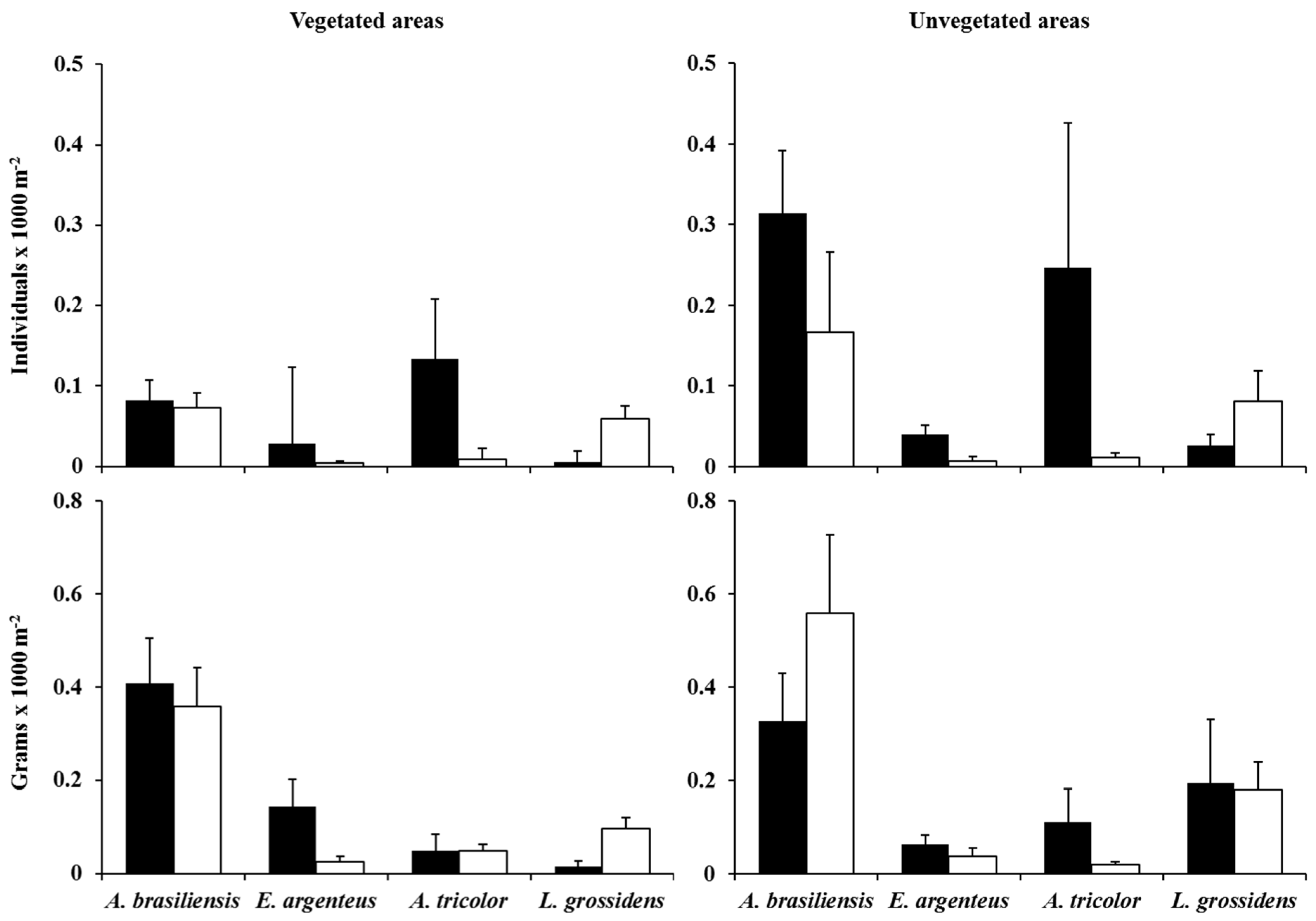
 ) Algae, (
 ) plant material, (
 ) Pennate diatomaceous, (
 ) Nematoda, (
 ) Trematoda, (
 ) Sedentary polychaeta, (
 ) Tubic Polychaeta, (
 ) Cyclopoida, (
 ) Calanoida, (
 ) Harpacticoida, (
 ) Brachyura zoea, (
 ) Cumacea, (
 ) Caprellidae, (
 ) Hymenoptera, (
 ) Gastropoda larvae, (
 ) Chaetognatha, (
 ) fish, (
 ) Fish—Gerreidae, (
 ) Fish—Engraulidae and (
 ) Fish—Mugilidae.
) Algae, () plant material, () Pennate diatomaceous, () Nematoda, () Trematoda, () Sedentary polychaeta, () Tubic Polychaeta, () Cyclopoida, () Calanoida, () Harpacticoida, () Brachyura zoea, () Cumacea, () Caprellidae, () Hymenoptera, () Gastropoda larvae, () Chaetognatha, () fish, () Fish—Gerreidae, () Fish—Engraulidae and () Fish—Mugilidae.
) Fish—Mugilidae.
) Algae, () plant material, () Pennate diatomaceous, () Nematoda, () Trematoda, () Sedentary polychaeta, () Tubic Polychaeta, () Cyclopoida, () Calanoida, () Harpacticoida, () Brachyura zoea, () Cumacea, () Caprellidae, () Hymenoptera, () Gastropoda larvae, () Chaetognatha, () fish, () Fish—Gerreidae, () Fish—Engraulidae and () Fish—Mugilidae.
 ) Algae, (
 ) plant material, (
 ) Pennate diatomaceous, (
 ) Nematoda, (
 ) Trematoda, (
 ) Sedentary polychaeta, (
 ) Tubic Polychaeta, (
 ) Cyclopoida, (
 ) Calanoida, (
 ) Harpacticoida, (
 ) Brachyura zoea, (
 ) Cumacea, (
 ) Caprellidae, (
 ) Hymenoptera, (
 ) Gastropoda larvae, (
 ) Chaetognatha, (
 ) fish, (
 ) Fish—Gerreidae, (
 ) Fish—Engraulidae and (
 ) Fish—Mugilidae.
) Algae, () plant material, () Pennate diatomaceous, () Nematoda, () Trematoda, () Sedentary polychaeta, () Tubic Polychaeta, () Cyclopoida, () Calanoida, () Harpacticoida, () Brachyura zoea, () Cumacea, () Caprellidae, () Hymenoptera, () Gastropoda larvae, () Chaetognatha, () fish, () Fish—Gerreidae, () Fish—Engraulidae and () Fish—Mugilidae.
) Fish—Mugilidae.
) Algae, () plant material, () Pennate diatomaceous, () Nematoda, () Trematoda, () Sedentary polychaeta, () Tubic Polychaeta, () Cyclopoida, () Calanoida, () Harpacticoida, () Brachyura zoea, () Cumacea, () Caprellidae, () Hymenoptera, () Gastropoda larvae, () Chaetognatha, () fish, () Fish—Gerreidae, () Fish—Engraulidae and () Fish—Mugilidae.
 ) and unvegetated areas (
 ), Eucinostomus argenteus in vegetated (●) and unvegetated areas (●), Anchoa tricolor in vegetated (▲) and unvegetated areas (▲), and Lycengraulis grossidens (LG) in vegetated (▼) and unvegetated areas (▼) of the estuary of the Mamanguape River, Northeastern Brazil, in 2014.
) and unvegetated areas (), Eucinostomus argenteus in vegetated (●) and unvegetated areas (●), Anchoa tricolor in vegetated (▲) and unvegetated areas (▲), and Lycengraulis grossidens (LG) in vegetated (▼) and unvegetated areas (▼) of the estuary of the Mamanguape River, Northeastern Brazil, in 2014.
), Eucinostomus argenteus in vegetated (●) and unvegetated areas (●), Anchoa tricolor in vegetated (▲) and unvegetated areas (▲), and Lycengraulis grossidens (LG) in vegetated (▼) and unvegetated areas (▼) of the estuary of the Mamanguape River, Northeastern Brazil, in 2014.
) and unvegetated areas (), Eucinostomus argenteus in vegetated (●) and unvegetated areas (●), Anchoa tricolor in vegetated (▲) and unvegetated areas (▲), and Lycengraulis grossidens (LG) in vegetated (▼) and unvegetated areas (▼) of the estuary of the Mamanguape River, Northeastern Brazil, in 2014.
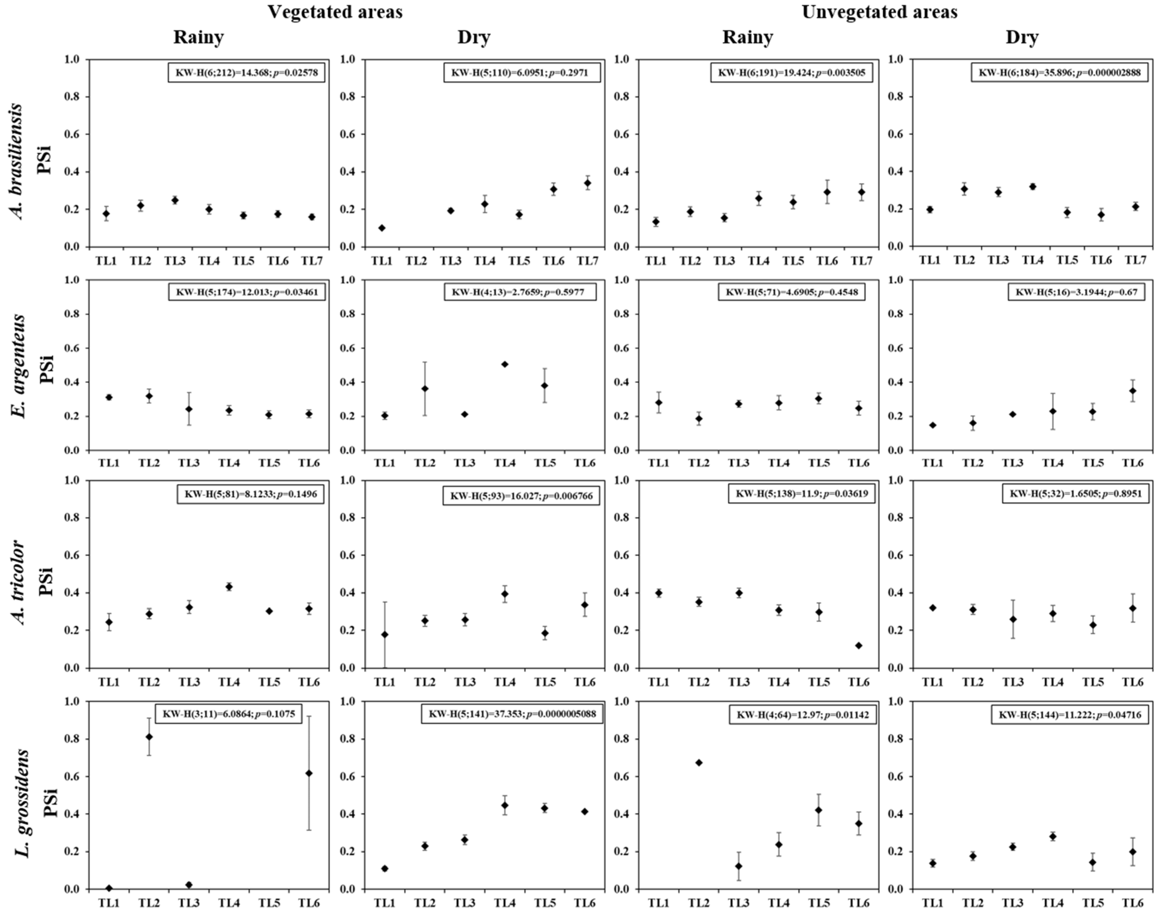
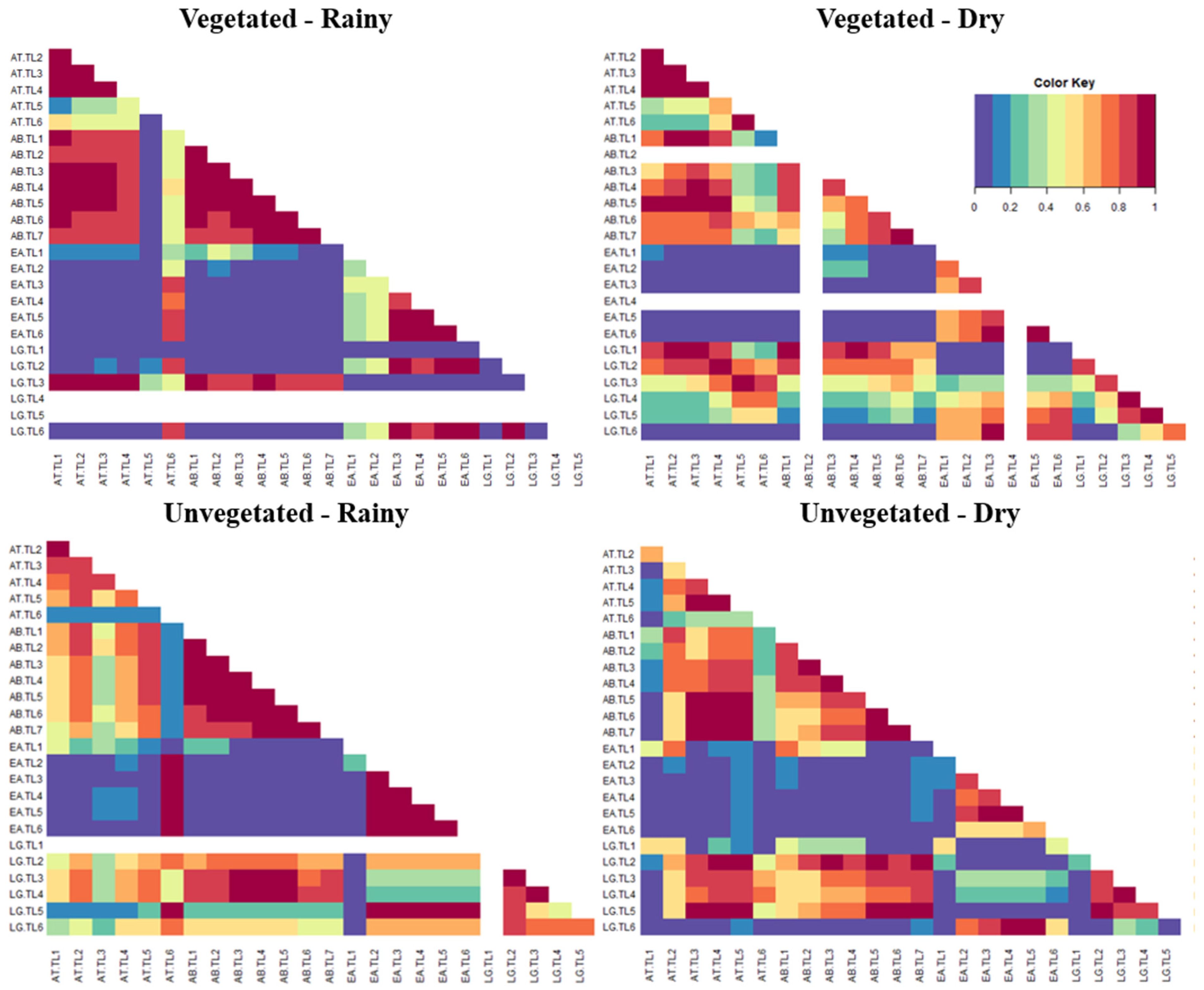
| Species | TL1 | TL2 | TL3 | TL4 | TL5 | TL6 | TL7 |
|---|---|---|---|---|---|---|---|
| Anchoa tricolor | ≤36 | 37–43 | 44–50 | 51–57 | 58–64 | ≥65 | - |
| Atherinella brasiliensis | ≤42 | 43–53 | 54–64 | 65–75 | 76–86 | 87–97 | ≥98 |
| Eucinostomus argenteus | ≤31 | 32–42 | 43–53 | 54–64 | 65–75 | ≥76 | - |
| Lycengraulis grossidens | ≤45 | 46–59 | 60–73 | 74–87 | 88–101 | ≥102 | - |
| Vegetated Areas | Unvegetated Areas | |||||||
|---|---|---|---|---|---|---|---|---|
| Rainy | Dry | Rainy | Dry | |||||
| Species | IS | n | IS | n | IS | n | IS | n |
| Atherinella brasiliensis | 0.190 * | 221 | 0.285 * | 110 | 0.206 * | 191 | 0.244 * | 184 |
| Eucinostomus argenteus | 0.281 * | 173 | 0.307 * | 14 | 0.272 * | 71 | 0.225 * | 16 |
| Anchoa tricolor | 0.302 * | 81 | 0.265 * | 93 | 0.368 * | 138 | 0.282 * | 32 |
| Lycengraulis grossidens | 0.399 * | 11 | 0.252 * | 142 | 0.298 * | 64 | 0.222 * | 144 |
| Vegetated Areas | Unvegetated Areas | |||
|---|---|---|---|---|
| Rainy | Dry | Rainy | Dry | |
| Species | H′ | H′ | H′ | H′ |
| Atherinella brasiliensis | 0.63 | 0.64 | 0.49 | 0.43 |
| Eucinostomus argenteus | 0.49 | 0.98 | 0.67 | 0.72 |
| Anchoa tricolor | 0.76 | 0.55 | 0.73 | 0.89 |
| Lycengraulis grossidens | 0.33 | 0.48 | 0.34 | 0.55 |
Disclaimer/Publisher’s Note: The statements, opinions and data contained in all publications are solely those of the individual author(s) and contributor(s) and not of MDPI and/or the editor(s). MDPI and/or the editor(s) disclaim responsibility for any injury to people or property resulting from any ideas, methods, instructions or products referred to in the content. |
© 2026 by the authors. Licensee MDPI, Basel, Switzerland. This article is an open access article distributed under the terms and conditions of the Creative Commons Attribution (CC BY) license.
Share and Cite
da Silva-Rodrigues, R.S.; Pessanha, A.L.M. Individual Variation in Diet of Four Fishes in Shallow Tropical Estuarine Areas: Comparisons Between Seasons and Habitats. Coasts 2026, 6, 24. https://doi.org/10.3390/coasts6020024
da Silva-Rodrigues RS, Pessanha ALM. Individual Variation in Diet of Four Fishes in Shallow Tropical Estuarine Areas: Comparisons Between Seasons and Habitats. Coasts. 2026; 6(2):24. https://doi.org/10.3390/coasts6020024
Chicago/Turabian Styleda Silva-Rodrigues, Rayssa Soares, and André Luiz Machado Pessanha. 2026. "Individual Variation in Diet of Four Fishes in Shallow Tropical Estuarine Areas: Comparisons Between Seasons and Habitats" Coasts 6, no. 2: 24. https://doi.org/10.3390/coasts6020024
APA Styleda Silva-Rodrigues, R. S., & Pessanha, A. L. M. (2026). Individual Variation in Diet of Four Fishes in Shallow Tropical Estuarine Areas: Comparisons Between Seasons and Habitats. Coasts, 6(2), 24. https://doi.org/10.3390/coasts6020024